Option pricing and hedging for regime-switching geometric Brownian motion models

Abstract.

We find the variance-optimal equivalent martingale measure when multivariate assets are modeled by a regime-switching geometric Brownian motion, and the regimes are represented by a homogeneous continuous time Markov chain. Under this new measure, the Markov chain driving the regimes is no longer homogeneous, which differs from the equivalent martingale measures usually proposed in the literature. We show the solution minimizes the mean-variance hedging error under the objective measure. As argued by Schweizer, (1996), the variance-optimal equivalent measure naturally extends canonical option pricing results to the case of an incomplete market and the expectation under the proposed measure may be interpreted as an option price. Solutions for the option value and the optimal hedging strategy are easily obtained from Monte Carlo simulations. Two applications are considered.

1. Introduction

Recently, regime-switching geometric Brownian motion (RSGBM) models have been the subject of much attention. They offer more flexibility than geometric Brownian motion models in capturing reported asset dynamics features such as time-varying volatility and high-order moments.

When the market is incomplete, as is the case for RSGBM models, there are infinitely many equivalent martingale measures to choose from, all free of arbitrage opportunities. Hence, arbitrage considerations alone cannot identify the measure and one has then to choose the “best” martingale measure according to some other criterion.

In many articles, e.g., Guo, (2001) and Shen et al., (2014) to name a few, options are evaluated under a parametrized family of martingale measures which are typically calibrated to historical option prices for empirical applications. However, the class of martingale measures proposed so far in the literature is quite limited. For example, in most cases, the distribution of the hidden regimes under the equivalent martingale measure is either unchanged or remains a time homogeneous Markov chain.

The main objective of this paper is to find (1) an equivalent martingale measure that is optimal in the sense of Schweizer, (1996), and (2) the optimal hedging strategy. More precisely, we find the equivalent signed martingale measure minimizing the variance of its density with respect to the objective measure, i.e. the so-called variance-optimal equivalent martingale measure. This first optimization problem is defined precisely in Section 2.2, while the second optimization problem pertaining to the mean-variance hedging is defined in Section 2.3. When prices are continuous, the variance-optimal measure is in fact a probability measure and expectations can be interpreted as arbitrage-free prices arising from a hedging strategy minimizing a mean-variance criterion for the (discounted) hedging error.

Our work is related to Černý and Kallsen, (2007) who show the existence of a solution for the optimal hedging problem under a very large class of models. For most cases of interest, their proposed solution is very difficult to find in practice. So far only a few cases have been solved in continuous time, including a very special stochastic volatility model (Černý and Kallsen,, 2008). For an implementable solution in discrete time, see, e.g., Rémillard and Rubenthaler, (2013)

In the next section, we describe the model and state the hedging problem. As in Shen et al., (2014), the instantaneous interest rate may vary with regimes. Then in Section 3, we propose a change of measure $\tilde{P}$, equivalent to the objective measure $P$, for which the discounted prices of assets are martingales. Under this martingale measure, the distribution of regimes becomes a time inhomogeneous Markov chain. We also define the forward measure and give representations for the associated option prices. The main results is that $\tilde{P}$ is variance-optimal. Next, in Section 4, we define a hedging strategy for the option price associated with the change of measure and we show that this hedging strategy minimizes the mean-variance hedging error. Finally, in Section 5, examples of computations are given, based on simulations and Fourier transforms.

2. Regime-switching model

We first define the model and then we state the hedging problem.

2.1. Model

Let $\tau$ be a continuous time Markov chain on $\{1,\ldots,l\}$, with infinitesimal generator $\Lambda$. In particular, $P(\tau_{t}=j|\tau_{0}=i)=P_{ij}(t)$, where the transition matrix $P$ can be written as $P(t)=e^{t\Lambda}$, $t\geq 0$. Then, the (continuous) price process $S$ is defined as the solution of the stochastic differential equation

$$dS_{t}=D(S_{t})\mu(\tau_{t})dt+D(S_{t})\sigma(\tau_{t-})dW_{t},$$ (2.1)

where $D(s)$ is the diagonal matrix with diagonal elements $(s_{j})_{j=1}^{d}$ and $W$ is a $d$-dimensional Brownian motion, independent of $\tau$. We set $(\mathcal{F}_{t}^{\tau})_{t\geq 0}$ for the filtration generated by $\tau$ and $(\mathcal{F}_{t}^{W})_{t\geq 0}$ for the filtration generated by $W$. It is assumed that $a(i)=\sigma(i)\sigma(i)^{\top}$ is invertible for any $i\in\{1,\ldots,l\}$. If $T_{\alpha}$ represents the time of the $\alpha-th$ jump of the regime process $\tau$, with $T_{0}=0$, then $S$ has the following representation for any $t\in[T_{\alpha-1},T_{\alpha}]$, $\alpha\geq 1$, given $\tau_{T_{\alpha-1}}=i$:

$$S_{t}^{(j)}=S_{T_{\alpha-1}}^{(j)}e^{\upsilon^{(j)}(i)(t-T_{\alpha-1})+\sum_{k=1}^{d}\sigma_{jk}(i)\left(W_{t}^{(k)}-W_{T_{\alpha-1}}^{(k)}\right)},\quad j\in\{1,\ldots,d\},$$ (2.2)

where $\upsilon(i)=\mu(i)-\frac{1}{2}{\rm diag}\{a(i)\}$, and ${\rm diag}(b)$ is the vector formed with the diagonal elements of the matrix $b$. Because of (2.2), such a process is called a ($d$-dimensional) regime-switching geometric Brownian motion with parameters $\mu(i),a(i)$, $i\in\{1,\ldots,l\}$. Note that $S$ is not a Markov process in general; however $(S,\tau)$ is a Markov process. One could also consider inhomogeneous Markov chains $\tau$, with an infinitesimal generator depending on time. See Appendix A for a possible construction. One may also define the law of $(S,\tau)$ through its infinitesimal generator $\mathcal{H}$, defined for all $f$ is in $C_{b}^{2}$ (the space of bounded continuous functions with bounded and continuous derivatives of order one and two) by

$$\mathcal{H}f(s,i)=\mathcal{L}_{i}f(s,i)+\sum_{j=1}^{l}\Lambda_{ij}f(s,j),$$ (2.3)

where for each $i=1,\ldots,l$ , $\mathcal{L}_{i}$ is the infinitesimal generator associated with the geometric Brownian motion with parameters $\mu(i),\sigma(i)$, defined by

$$\mathcal{L}_{i}f(s)=\mu(i)^{\top}D(s)\nabla f(s)+\frac{1}{2}\sum_{k=1}^{d}\sum_{j=1}^{d}a_{kj}(i)s_{k}s_{j}\partial_{s_{k}}\partial_{s_{j}}f(s).$$

The main property of the infinitesimal generator $\mathcal{L}$ of a Markov process $x_{t}$ that will be used is that $f(x_{t})-\int_{0}^{t}\mathcal{L}f(x_{u})du$ is a martingale. For more details, see, e.g., Ethier and Kurtz, (1986). To be able to compare our results with those of Shen et al., (2014), we assume that the instantaneous interest rate at time $t$ is given by $r_{\tau_{t-}}$, with $r\in[0,\infty)^{l}$. The (random) discounting factor $B$ is then given by

$$B_{t}=e^{-\int_{0}^{t}r_{\tau_{u}}du},\quad t\geq 0,$$ (2.4)

so that $X_{t}=B_{t}S_{t}$ is the discounted price process.

We now describe the two optimization problems we want to solve in this paper.

2.2. Variance-optimal martingale measure

As defined in Schweizer, (1996), let $\mathcal{Q}$ be the set of all absolutely continuous signed martingale measures $Q$ with respect to $P$, having a square integrable density $Z_{t}=\left.\frac{dQ}{dP}\right|_{\mathcal{F}_{t}}$, so that for all $t\in[0,T]$, $E(Z_{t})=1$, and $X_{t}Z_{t}$ is a $P$-martingale. Then $\tilde{P}\in\mathcal{Q}$ is variance-optimal if

$$E\left[\left(\left.\frac{d\tilde{P}}{dP}\right|_{\mathcal{F}_{T}}\right)^{2}\right]=\inf_{Q\in\mathcal{Q}}E\left[\left(\left.\frac{d\tilde{P}}{dP}\right|_{\mathcal{F}_{T}}\right)^{2}\right].$$

In Schweizer, (1996), it was shown that the variance-optimal measure exists, is unique and it is indeed a true probability measure if $X$ is continuous, which is the case here.

One of the main aim of this paper is to find the variance-optimal martingale measure for the RSGBM model. This is done in Lemma 3.5.

2.3. Hedging problem

The other motivation of the paper is to solve a quadratic hedging problem for the price process $S$. More precisely, let $\mathcal{A}$ be the class of admissible strategies $\psi$ defined as the $L^{2}(P)$ closure of (finite) linear combination of simple admissible strategies $\psi$ of the form $\psi=Y\mathbb{I}_{(T_{1},T_{2}]}$, where $T_{1},T_{2}$ are stopping times so that $0\leq T_{1}\leq T_{2}\leq T$, and $Y$ is a bounded random vector that is $\mathcal{F}_{T_{1}}$-measurable. Note that the class of admissible strategies is a bit different from the one considered by Černý and Kallsen, (2007). The (quadratic) hedging problem for the regime-switching geometric Brownian motion is to minimize the discounted quadratic hedging error defined by

$$\mathit{HE}(\pi,\psi)=E\left[\left\{B_{T}\Phi(S_{T})-\pi-\int_{0}^{T}\psi_{u}^{\top}dX_{u}\right\}^{2}\right],\quad(\pi,\psi)\in\mathbb{R}\times\mathcal{A},$$ (2.5)

where $X_{t}=B_{t}S_{t}$ is the discounted price process. Here, $\pi$ is the initial value of the portfolio, and $\pi+\int_{0}^{T}\psi_{u}^{\top}dX_{u}$ is its discounted value at time $t\geq 0$.

In the next section, we propose a candidate for the variance-optimal equivalent martingale measure. It was shown in Schweizer, (1996) that for the variance-optimal equivalent martingale measure $\hat{P}$, if for a given $\Phi$, $(C_{0},\varphi)$ minimizes (2.5), then $C_{0}=E^{\hat{P}}[B_{T}\Phi(S_{T})]$.

3. Change of measures and off-line computations

In order to be able to define the proposed change of measures, we need to introduce auxiliary deterministic functions. This is done next in Section 3.1, after introducing first some notations.

For $i\in\{1,\ldots,l\}$, let $m(i)=(\mu(i)-r_{i}\mathbf{1})$, $\rho(i)=a(i)^{-1}m(i)$, and set

$$\ell_{i}=\rho(i)^{\top}m(i)=m(i)^{\top}a(i)^{-1}m(i)=\rho(i)^{\top}a(i)\rho(i)\geq 0.$$ (3.1)

As a result, one obtains the following representation for the discounted value $X$ of $S$:

$$X_{t}=B_{t}S_{t}=S_{0}+\int_{0}^{t}D(X_{u})m(\tau_{u})du+\int_{0}^{t}D(X_{u})\sigma(\tau_{u-})dW_{u},\quad t\geq 0.$$ (3.2)

We now define the deterministic functions that plays a central role in the change of maesures.

3.1. Auxiliary functions

Let $\gamma(t)=e^{t\{\Lambda-D(\ell)\}}\mathbf{1}$ and $\delta(t)=e^{t\{\Lambda-D(\ell+r)\}}\mathbf{1}$. Then, for all $i\in\{1,\ldots,l\}$, $\gamma_{i}(0)=1$, $\delta_{i}(0)=1$, and

$$\dot{\gamma}_{i}(t) = \frac{d}{dt}\gamma_{i}(t)=-\ell_{i}\gamma_{i}(t)+\sum_{j=1}^{l}\Lambda_{ij}\gamma_{j}(t),$$ (3.3)

$$\dot{\delta}_{i}(t) = \frac{d}{dt}\delta_{i}(t)=-(\ell_{i}+r_{i})\delta_{i}(t)+\sum_{j=1}^{l}\Lambda_{ij}\delta_{j}(t).$$ (3.4)

The following lemma, proven in Appendix B.1, gives other representations for $\gamma$ and $\delta$.

Lemma 3.1.

Let $\gamma$ and $\delta$ be the solutions of (3.3) and (3.4). Then for all $t\geq 0$ and for all $i\in\{1,\ldots,l\}$, $1\geq\gamma_{i}(t)\geq e^{(\Lambda_{ii}-\ell_{i})t}>0$, $1\geq\delta_{i}(t)\geq e^{(\Lambda_{ii}-\ell_{i}-r_{i})t}>0$, and

$$\gamma_{i}(t) = E_{i}\left[e^{-\int_{0}^{t}\ell_{\tau_{u}}du}\right],$$ (3.5)

$$\delta_{i}(t) = E_{i}\left[e^{-\int_{0}^{t}\left(r_{\tau_{u}}+\ell_{\tau_{u}}\right)du}\right].$$ (3.6)

Next, by Lemma 3.1, for any $t\geq 0$ and any $i\in\{1,\ldots,l\}$, $\gamma_{i}(t)>0$ and $\delta_{i}(t)>0$, so one may define $\beta_{i}(t)=\delta_{i}(t)/\gamma_{i}(t)$, and

$$(\tilde{\Lambda}_{t})_{ij} = \Lambda_{ij}\gamma_{j}(t)/\gamma_{i}(t),\quad i\neq j,\qquad(\tilde{\Lambda}_{t})_{ii}=-\sum_{j\neq i}(\tilde{\Lambda}_{t})_{ij},$$ (3.7)

$$\left(\stackrel{{\scriptstyle\circ}}{{\Lambda}}_{t}\right)_{ij} = \frac{\Lambda_{ij}\delta_{j}(t)}{\delta_{i}(t)}=\frac{(\tilde{\Lambda}_{t})_{ij}\beta_{j}(t)}{\beta_{i}(t)},\quad i\neq j,\qquad\left(\stackrel{{\scriptstyle\circ}}{{\Lambda}}_{t}\right)_{ii}=-\sum_{j\neq i}\left(\stackrel{{\scriptstyle\circ}}{{\Lambda}}_{t}\right)_{ij}.$$ (3.8)

Then $\tilde{\Lambda}_{t}$, $t\in[0,T]$, is the infinitesimal generator of a time inhomogeneous Markov chain. The same is true for $\stackrel{{\scriptstyle\circ}}{{\Lambda}}_{t}$, $t\in[0,T]$.

Remark 3.2.

It follows from Lemma 3.1 that $\beta_{i}(0)=1$, and that for any $t>0$,

$$\beta_{i}(t)=\frac{E_{i}\left[e^{-\int_{0}^{t}(r_{\tau_{u}}+\ell_{\tau_{u}})du}\right]}{\gamma_{i}(t)},$$ (3.9)

and

$$\dot{\beta}_{i}(t)=\frac{d}{dt}\beta_{i}(t)=-r_{i}\beta_{i}(t)+(\tilde{\Lambda}_{t})_{ii}\beta_{i}(t)-\left(\stackrel{{\scriptstyle\circ}}{{\Lambda}}_{t}\right)_{ii}\beta_{i}(t),\quad t>0.$$ (3.10)

Note that if $r$ is constant, then $\beta_{i}(t)=B_{t}$ and $\stackrel{{\scriptstyle\circ}}{{\Lambda}}_{t}=\tilde{\Lambda}_{t}$ for any $t\geq 0$.

3.2. Change of measure

Set $M_{t}=\int_{0}^{t}\rho(\tau_{u-})^{\top}D^{-1}(X_{u})dX_{u}$, $t\geq 0$. Then,

$$M_{t}=\int_{0}^{t}\ell_{\tau_{u}}du+\int_{0}^{t}\rho(\tau_{u-})^{\top}\sigma(\tau_{u-})dW_{u}=\int_{0}^{t}\ell_{\tau_{u}}du+\mathcal{M}_{t},\quad t\geq 0,$$ (3.11)

where $\mathcal{M}$ is a martingale with quadratic variation $[\mathcal{M},\mathcal{M}]_{t}=[M,M]_{t}=\int_{0}^{t}\ell_{\tau_{u}}du$, using (3.1) and (3.2). For $t\geq 0$, further set

$$Z_{t}=\mathcal{E}_{t}\left\{-M\right\}=e^{-M_{t}-\frac{1}{2}[M,M]_{t}}=\mathcal{E}_{t}\left\{-\mathcal{M}\right\}e^{-\int_{0}^{t}\ell_{\tau_{u}}du}=Z_{t}^{(1)}e^{-\int_{0}^{t}\ell_{\tau_{u}}du},$$

where $\mathcal{E}$ is the stochastic exponential; see, e.g., Protter, (2004, page 85). We are now in a position to define the change of measure. The proof is given in Appendix C.1. Note that this change of measure can be obtained as a limit of the discrete case (Schweizer,, 1995, Rémillard and Rubenthaler,, 2013) when the number of hedging periods tends to infinity.

Lemma 3.3.

$Z$ is a multiplicative functional, and the processes $Z_{t}^{(1)}=e^{-\mathcal{M}_{t}-\frac{1}{2}[\mathcal{M},\mathcal{M}]_{t}}$ and $Z_{t}^{(2)}=\gamma_{\tau_{t}}(T-t)e^{-\int_{0}^{t}\ell_{\tau_{u}}du}$ are positive orthogonal martingales. Moreover, $E(Z_{T}|\mathcal{F}_{t})=Z_{t}^{(1)}Z_{t}^{(2)}=Z_{t}\gamma_{\tau_{t}}(T-t)$ and $\gamma_{i}(t)=E_{i}(Z_{t})$, for all $t\geq 0$. Also, $\left.\frac{d\tilde{P}}{dP}\right|_{\mathcal{F}_{T}}=Z_{T}/\gamma_{\tau_{0}}(T)=Z_{T}^{(1)}Z_{T}^{(2)}/\gamma_{\tau_{0}}(T)$ defines an equivalent change of measure, and for any $t\in[0,T]$,

$$\left.\frac{d\tilde{P}}{dP}\right|_{\mathcal{F}_{t}}=Z_{t}\gamma_{\tau_{t}}(T-t)/\gamma_{\tau_{0}}(T)=Z_{t}^{(1)}Z_{t}^{(2)}/\gamma_{\tau_{0}}(T).$$ (3.12)

Under $\tilde{P}$, $\tau$ is an inhomogeneous Markov chain with generator $\tilde{\Lambda}_{T-t}$, $\tilde{W}_{t}=W_{t}+\int_{0}^{t}\sigma_{\tau_{u}}^{\top}\rho_{\tau_{u}}du$ is a Brownian motion independent of $\tau$, and $X$ is a $\tilde{P}$-martingale. As a result, under $\tilde{P}$, $(S,\tau)$ has infinitesimal generator $\tilde{\mathcal{H}}_{t}$ given by

$${\tilde{\mathcal{H}}}_{t}f(s,i)=\tilde{\mathcal{L}}_{i}f(s,i)+\sum_{j=1}^{l}(\tilde{\Lambda}_{T-t})_{ij}f(s,j),\quad t\in[0,T],$$ (3.13)

with

$$\tilde{\mathcal{L}}_{i}f(s,i)=r_{i}\sum_{k=1}^{d}s_{k}\partial_{s_{k}}f(s,i)+\frac{1}{2}\sum_{j=1}^{d}\sum_{k=1}^{d}a_{jk}(i)s_{j}s_{k}\partial_{s_{j}}\partial_{s_{k}}f(s,i).$$ (3.14)

Remark 3.4.

Note that $Z^{(1)}$ corresponds to the density of the so-called “minimal martingale measure” Föllmer and Schweizer, (1991), which is different from the (unnormalized) density $Z^{(1)}Z^{(2)}$. This is a non-trivial example of the difference between local risk-minimizing strategies, as considered in Föllmer and Schweizer, (1991), and global risk-minimizing strategies, as considered here.

The main result of this section is stated next, and it is proven in Appendix C.2.

Lemma 3.5.

$\tilde{P}$ is the variance-optimal equivalent martingale measure, as defined in Section 2.2.

The following proposition defines the so-called forward measure, which is necessary only when the interest rate is stochastic. The proof of the proposition is similar to the proof of Lemma 3.3 so it is omitted.

Proposition 3.6.

For any $t\in[0,T]$, $E^{\tilde{P}}\left[\left.B_{T}\right|\mathcal{F}_{t}\right]=B_{t}\beta_{\tau_{t}}(T-t)$. As a result,

$$\left.\frac{d\stackrel{{\scriptstyle\circ}}{{P}}}{d\tilde{P}}\right|_{\mathcal{F}_{T}}=B_{T}/\beta_{\tau_{0}}(T)$$ (3.15)

defines the forward measure, and for any $t\in[0,T]$, $\left.\frac{d\stackrel{{\scriptstyle\circ}}{{P}}}{d\tilde{P}}\right|_{\mathcal{F}_{t}}=\frac{\beta_{\tau_{t}}(T-t)}{\beta_{\tau_{0}}(T)}B_{t}$. Under $\stackrel{{\scriptstyle\circ}}{{P}}$, $\tau$ is an inhomogeneous Markov chain with generator $\stackrel{{\scriptstyle\circ}}{{\Lambda}}_{T-t}$, $\stackrel{{\scriptstyle\circ}}{{W}}_{t}=W_{t}+\int_{0}^{t}\sigma_{\tau_{u}}^{\top}\rho_{\tau_{u}}du$ is a Brownian motion independent of $\tau$, and $\left(S_{t}/\beta_{\tau_{t}}(T-t)\right)_{t\in[0,T]}$ is a $\stackrel{{\scriptstyle\circ}}{{P}}$-martingale. Moreover, under $\stackrel{{\scriptstyle\circ}}{{P}}$, $(S,\tau)$ has infinitesimal generator $\stackrel{{\scriptstyle\circ}}{{\mathcal{H}}}_{t}$ given by

$$\stackrel{{\scriptstyle\circ}}{{\mathcal{H}}}_{t}f(s,i)=\tilde{\mathcal{L}}_{i}f(s,i)+\sum_{j=1}^{l}\left(\stackrel{{\scriptstyle\circ}}{{\Lambda}}_{T-t}\right)_{ij}f(s,j).$$

3.3. Option price under $\tilde{P}$

Suppose that the payoff $\Phi$ is of polynomial order. Under $\tilde{P}$ defines in Lemma 3.3, the value of a European option with payoff $\Phi$ at maturity $T$ is

$$C_{t}(S_{t},\tau_{t})=E^{\tilde{P}}\left[e^{-\int_{t}^{T}r_{\tau_{u}}du}\;\Phi(S_{T})|\mathcal{F}_{t}\right]=\frac{E\left[B_{T}Z_{T}\;\Phi(S_{T})|\mathcal{F}_{t}\right]}{B_{t}Z_{t}\gamma_{\tau_{t}}(T-t)}.$$ (3.16)

Since $Z$ is a multiplicative functional by Lemma 3.3, $C$ can also be written as

$$C_{t}(s,i)=E_{s,i}\left[B_{T-t}Z_{T-t}\Phi(S_{T-t})\right]\Big{/}\gamma_{i}(T-t).$$ (3.17)

The next result, proven in Appendix A.1, shows that option prices are smooth.

Proposition 3.7.

The density $f_{s,t}(y)$ of $S_{t}$ is infinitely differentiable with respect to $s$ and $y$, and continuously differentiable with respect to $t$ if ${\tilde{\Lambda}}_{t}$ is. Moreover all these derivatives are integrable and the density possesses moments of all orders.

Note that by Proposition 3.7, $C_{t}(s,i)$ is continuously differentiable with respect to $t$, and twice continuously differentiable with respect to $s\in(0,\infty)^{d}$, for any $t<T$. The next result, which follows from the definition of $C$ together with Lemma 3.3 and Proposition 3.6, gives two more representations for $C$.

Lemma 3.8.

Let $C$ be given by (3.16). If $(\tilde{S},\tilde{\tau})$ has infinitesimal generator $\tilde{\mathcal{H}}_{t}$, then

$$C(t,s,i)=E\left[e^{-\int_{t}^{T}r_{\tilde{\tau}_{u}}du}\;\Phi(\tilde{S}_{T})|\tilde{S}_{t}=s,\tilde{\tau}_{t}=i\right].$$ (3.18)

Also, if $\left(\stackrel{{\scriptstyle\circ}}{{S}},\stackrel{{\scriptstyle\circ}}{{\tau}}\right)$ is a process with generator $\stackrel{{\scriptstyle\circ}}{{\mathcal{H}}}_{t}$, then

$$C(t,s,i)=\beta_{i}(T-t)E\left[\Phi\left(\stackrel{{\scriptstyle\circ}}{{S}}_{T}\right)|\stackrel{{\scriptstyle\circ}}{{S}}_{t}=s,\stackrel{{\scriptstyle\circ}}{{\tau}}_{t}=i\right].$$ (3.19)

Remark 3.9.

Under the assumptions on $\Phi$, it follows from Proposition 3.7 that $C$ is smooth, and an application of Ito’s formula yields that $C$ satisfies

$$\partial_{t}C_{t}(s,i)+{\tilde{\mathcal{H}}}_{t}C_{t}(s,i)=r_{i}C_{t}(s,i),\quad C_{T}(s,i)=\Phi(s).$$ (3.20)

Remark 3.10.

Note that using the Algorithm 1 described in Appendix A, together with (3.19), it is easy to use a Monte-Carlo method to estimate $C_{t}$.

3.4. Call option

For the remaining of the section, suppose that $d=1$ and consider the European call option payoff $\Phi(s)=\max(0,s-K)$. We show below that as in the Black-Scholes case, one can write the price $C$ of the option using only the distribution function of the log-return $\log{S_{T}}$ under the forward measure $\stackrel{{\scriptstyle\circ}}{{P}}$ and another measure obtained by a Esscher transform. These distribution functions could be possibly computed by inverting their Laplace transforms or their characteristic functions. See Appendix D for the corresponding formulas. First, we define the Esscher transform using the fact that

$$E^{\stackrel{{\scriptstyle\circ}}{{P}}}\left[S_{T}|\mathcal{F}_{t}\right] = \frac{E^{\tilde{P}}\left[e^{-\int_{t}^{T}r_{\tau_{u}}du}\;S_{T}|\mathcal{F}_{t}\right]}{E^{\tilde{P}}\left[e^{-\int_{t}^{T}r_{\tau_{u}}du}|\mathcal{F}_{t}\right]}=\frac{S_{t}}{\beta_{\tau_{t}}(T-t)}.$$

We introduce the change of measure by setting $\left.\frac{d\check{P}}{d\stackrel{{\scriptstyle\circ}}{{P}}}\right|_{\mathcal{F}_{T}}=\frac{S_{T}}{E^{\stackrel{{\scriptstyle\circ}}{{P}}}\left(S_{T}\right)}$. Next, according to (3.19),

$$C_{t}(s,i) = s\frac{E^{\stackrel{{\scriptstyle\circ}}{{P}}}\left[S_{T}\mathbb{I}\left(S_{T}>K\right)|S_{t}=s,\tau_{t}=i\right]}{E^{\stackrel{{\scriptstyle\circ}}{{P}}}\left[S_{T}|S_{t}=s,\tau_{t}=i\right]}-\beta_{i}(T-t)K{\stackrel{{\scriptstyle\circ}}{{P}}}\left[S_{T}>K|S_{t}=s,{\tau}_{t}=i\right]$$ (3.21)

$$= s\check{P}\left[S_{T}>K|S_{t}=s,\tau_{t}=i\right]-\beta_{i}(T-t)K{\stackrel{{\scriptstyle\circ}}{{P}}}\left[S_{T}>K|S_{t}=s,{\tau}_{t}=i\right].$$

Furthermore, if for a given $t$, $\stackrel{{\scriptstyle\circ}}{{f}}$ is the conditional density of $\log\left(S_{T}/s\right)$ given $S_{t}=s,\tau_{t}=i$ under $\stackrel{{\scriptstyle\circ}}{{P}}$, and if $\check{f}$ is the conditional density of $\log\left(S_{T}/s\right)$ given $S_{t}=s,\tau_{t}=i$ under $\check{P}$, then $\check{f}(x)=\beta_{i}(T-t)e^{x}\stackrel{{\scriptstyle\circ}}{{f}}(x)$, so using (3.21), one finds

$$\partial_{s}C_{t}(s,i) = \check{P}\left[S_{T}>K|S_{t}=s,\check{\tau}_{t}=i\right]+\check{f}\{\log(K/s)\}-\beta_{i}(T-t)\frac{K}{s}\stackrel{{\scriptstyle\circ}}{{f}}\{\log(K/s)\}$$

$$= \check{P}\left[S_{T}>K|S_{t}=s,\tau_{t}=i\right].$$

It only remains to find the distribution of $(S,\tau)$ under $\check{P}$. This is done in the next Lemma, whose proof is given in Appendix C.3.

Lemma 3.11.

Under the change of measure $\left.\frac{d\check{P}}{d\stackrel{{\scriptstyle\circ}}{{P}}}\right|_{\mathcal{F}_{T}}=\frac{S_{T}}{E^{\stackrel{{\scriptstyle\circ}}{{P}}}\left(S_{T}\right)}$, $\left(S,\tau\right)$ has infinitesimal generator $\tilde{\mathcal{H}}_{t}$ defined by $\check{\mathcal{H}}_{t}f(s,i)=\check{\mathcal{L}}_{i}f(s,i)+\tilde{\Lambda}_{T-t}f(s,i)$, where for any smooth $f$,

$$\check{\mathcal{L}}_{i}f(s,i)=(r_{i}+a_{i})s\partial_{s}f(s,i)+\frac{a_{i}}{2}s^{2}\partial_{s}^{2}f(s,i),\quad i\in\{1,\ldots,l\}.$$

Having defined the price of the option under the equivalent martingale measure $\tilde{P}$, we are now in a position to find the optimal strategy $(\pi,\psi)\in\mathbb{R}\times\mathcal{A}$ minimizing the quadratic hedging error $\mathit{HE}(\pi,\psi)$. This is the content of the next section.

4. Optimal hedging strategy

Let $C$ be defined by (3.17), and set

$$\alpha_{t}(s,i)=\nabla_{s}C_{t}(s,i)+C_{t}(s,i)D^{-1}(s)\rho(i).$$ (4.1)

Further let $V$ be the solution of the stochastic differential equation

$$V_{t}=C_{0}(s,i)+\int_{0}^{t}\alpha_{u}(S_{u},\tau_{u-})^{\top}dX_{u}-\int_{0}^{t}V_{u-}dM_{u},\quad(S_{0},\tau_{0})=(s,i),$$ (4.2)

which exists and is unique, according to Protter, (2004, Theorem V.7). The proof of the following lemma is given in Appendix C.4.

Lemma 4.1.

Define $G_{t}=B_{t}C_{t}(S_{t},\tau_{t})-V_{t}$, and set

$$\phi_{t} = \alpha_{t}(S_{t},\tau_{t-})-V_{t-}D^{-1}(X_{t})\rho(\tau_{t-})$$ (4.3)

$$= \nabla_{s}C_{t}(S_{t},\tau_{t-})+G_{t-}D^{-1}(X_{t})\rho(\tau_{t-}).$$ (4.4)

Then $\phi$ is predictable and

$$V_{t}=C_{0}(S_{0},\tau_{0})+\int_{0}^{t}\phi_{u}^{\top}dX_{u},$$ (4.5)

Equation (4.5) shows that $V_{t}$ is the discounted value at time $t$ of a portfolio with initial value $C_{0}(s,i)$ and investment strategy $\phi$, so $G_{t}$ is the corresponding hedging error at this period. Recall that $C_{0}=E^{\tilde{P}}[B_{T}\Phi(S_{T})]$ is a real option price, corresponding to the price under the variance-optimal martingale measure $\tilde{P}$. In other words, if all agents in the economy minimize a mean-variance criterion for the hedging error under a RSGBM model, then the pricing kernel will be generated by the variance-optimal measure $\tilde{P}$.

It is interesting to note that $\phi_{0}=\nabla_{s}C_{0}(s,i)$, but in general, $\phi_{t}\neq\nabla_{s}C_{t}(S_{t},\tau_{t-})$, unless $G_{t-}=0$, indicating perfect hedging.

Remark 4.2.

Since $\alpha_{t}(s,i)=\nabla_{s}C_{t}(s,i)+C_{t}(s,i)D^{-1}(s)\rho(i)$, $i\in\{1,\ldots,l\}$, one can obtain an unbiased estimate of $\alpha_{t}$ through simulations by using an obvious extension of the “pathwise method” in Broadie and Glasserman, (1996). More precisely, if $\Phi$ is differentiable almost everywhere, then (3.19) yields

$$\nabla_{s}C_{t}(s,i)=\beta_{i}(T-t)D^{-1}(s)E^{\stackrel{{\scriptstyle\circ}}{{P}}}\left[D(S_{T})\nabla\Phi(S_{T})|S_{t}=s,\tau_{t}=i\right],$$ (4.6)

so $\alpha_{t}$ is an expectation of a function of $S_{T}$. It follows from (4.3) and (4.6) that $\phi_{t}$ can also be estimated by Monte-Carlo methods.

Next, we find an expression for the hedging error $G$ of the investment strategy $(C_{0},\phi)$. It’s proof is given in Appendix C.5.

Lemma 4.3.

The hedging error $G$ satisfies

$$G_{t}=-\int_{0}^{t}G_{u-}dM_{u}+\sum_{0<u\leq t}B_{u}\Delta C_{u}(S_{u},\tau_{u})-\int_{0}^{t}B_{u}\tilde{\Lambda}_{T-u}C_{u}(S_{u},\tau_{u})du.$$ (4.7)

The next result, proven in Appendix C.6, is the key for solving the hedging problem.

Lemma 4.4.

For all $0\leq t\leq T$, $\gamma_{\tau_{t}}(T-t)G_{t}$ and $\gamma_{\tau_{t}}(T-t)X_{t}G_{t}$ are martingales. In particular $E(G_{T})=0$, and for any stopping times $U,V$ with $0\leq U\leq V\leq T$,

$$E\left\{G_{T}(X_{V}-X_{U})|\mathcal{F}_{U}\right)=0.$$ (4.8)

One can now state the other main result of the paper, proven in Appendix C.7. Recall that the quadratic hedging error $\mathit{HE}$ is defined in (2.5).

Theorem 4.5.

The optimal solution of the quadratic hedging problem for a regime-switching geometric Brownian motion is given by $(C_{0},\phi)$, as defined by equation (4.3) and the actualized value of the associated portfolio satisfies (4.2). More precisely, for any $(\pi,\psi)\in\mathbb{R}\times\mathcal{A}$,

$$\mathit{HE}(\pi,\psi)\geq\mathit{HE}(C_{0},\phi),$$ (4.9)

and $\mathit{HE}(\pi,\psi)=\mathit{HE}(C_{0},\phi)$ if and only if $\pi=C_{0}$ and $\psi=\phi$ a.s. In particular, the solution to the optimization problem exists and is unique.

4.1. Particular cases

4.1.1. Geometric Brownian motion

In this case, $\Lambda\equiv 0$ and $C$ does not depend on $\tau$, so by Lemma 4.3, $G_{t}=-\int_{0}^{t}G_{u}dM_{u}$, with $G_{0}=0$. Since the solution of (4.7) is unique, $G\equiv 0$, proving the perfect hedging, as it is well-known for the Black-Scholes model. Also, using (4.4), one recovers the delta-hedging value $\phi_{t}=\nabla_{s}C_{t}(S_{t})$.

4.1.2. Risk neutral measure

To recover known results from the literature, suppose that $X_{t}=B_{t}S_{t}$ is a martingale. It then follows from (3.2) that $m\equiv 0$, so $\rho\equiv 0$, $\ell\equiv 0$, $\gamma\equiv 1$, ${\tilde{\mathcal{H}}}_{t}=\mathcal{H}$, $M\equiv 0$, and $Z\equiv 1$. Next, we get from (3.18), (4.1) – (4.3) that

$$C_{t}(s,i) = E\left\{B_{T-t}\Phi(S_{T-t})|S_{0}=s,\tau_{0}=i\right\},$$

$$\alpha_{t}(,s,i) = \nabla C_{t}(s,i),$$

$$V_{t} = C_{0}(s,i)+\int_{0}^{t}\alpha_{u}(S_{u},\tau_{u-})^{\top}dX_{u},$$

$$\phi_{t} = \alpha_{t}(S_{t-},\tau_{t-}).$$

5. Examples of application

In this section, we present two implementations of our proposed methodology, using formulas (3.19) and (4.6) together with Monte Carlo simulations to estimate respectively the value of an option and the initial investment in the risky asset. The simulations are based on Algorithm 1 described in Appendix A.

5.1. A first example

In Shen et al., (2014), the authors consider a RSGBM with parameters $\mu=(0.04,0.08)^{\top}$, $\sigma=(0.4,0.2)^{\top}$, $r=(0.02,0.04)^{\top}$ and generator $\Lambda=0.5\left(\begin{array}[]{rr}-1&1\\ 1&-1\end{array}\right)$. Also, $S_{0}=100$, $T=1$. Note that under their risk neutral measure, the regime-switching process $\tau$ is still time-homogeneous. In order to be able to make some comparisons with our model, only their SRS model is chosen. Using inverse Fourier transforms, they obtained the value of call options given in Table 1.

Table 1. Call option prices computed with a discretization of $2^{12}$ points for the inverse Fourier transform (Shen et al.,, 2014).

Strike	70	80	90	100	110	120
Regime 1	34.0904	26.7779	20.6144	15.6171	11.6953	8.6931
Regime 2	33.1151	24.5557	17.1617	11.3358	7.1553	4.3873

In order to implement our proposed methodology using Monte Carlo simulations, one has to find $\lambda=\max_{i\in\{1,2\}}\sup_{t\in[0,1]}-\left(\stackrel{{\scriptstyle\circ}}{{\Lambda}}_{t}\right)_{ii}$, as described in Algorithm 1. Based on panel (a) in Figure 1, one can take $\lambda=.5185$. Note also that the discounting factors $\beta_{i}(T)$ are given by $0.9767$ for regime 1 and $0.9644$ for regime 2. Their values are displayed in panel (b) of Figure 1. Next, in Table 2, 95% confidence intervals are computed for the call values and the initial investment $\phi_{0}$ (number of shares), based on $10^{6}$ simulated values of $\stackrel{{\scriptstyle\circ}}{{S}}_{T}$. Although the model proposed by Shen et al., (2014) and our model are different under the martingale measures, the option values obtained from both models are comparable. However, one can see that under regime 1, our results are significantly lower than those of Shen et al., (2014), while they are significantly larger for regime 2. Estimated call values and $\phi_{0}$ for the two regimes are displayed in Figure 2 for strike ranging from $50$ to $150$.

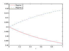
(a) (b)

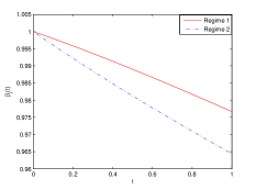
Figure 1. Graphs of $-\left(\stackrel{{\scriptstyle\circ}}{{\Lambda}}_{t}\right)_{ii}$ (panel a) and $\beta_{i}(t)$ (panel b), for $i\in\{1,2\}$.

Table 2. Call option prices and initial investment values computed by Monte Carlo with $10^{6}$ simulations, using antithetic variables.

	Call value		Initial value $\phi_{0}$
Strike	Regime 1	Regime 2	Regime 1	Regime 2
70	$34.0580\pm 0.0489$	$33.1345\pm 0.0347$	$0.8935\pm 0.0007$	$0.9547\pm 0.0005$
80	$26.6933\pm 0.0460$	$24.6400\pm 0.0328$	$0.8112\pm 0.0008$	$0.8863\pm 0.0006$
90	$20.4806\pm 0.0424$	$17.3062\pm 0.0299$	$0.7103\pm 0.0009$	$0.7672\pm 0.0008$
100	$15.4499\pm 0.0384$	$11.5217\pm 0.0262$	$0.6005\pm 0.0010$	$0.6111\pm 0.0008$
110	$11.5158\pm 0.0343$	$\phantom{1}7.3565\pm 0.0222$	$0.4931\pm 0.0010$	$0.4492\pm 0.0009$
120	$\phantom{1}8.5192\pm 0.0303$	$\phantom{1}4.5829\pm 0.0184$	$0.3958\pm 0.0009$	$0.3095\pm 0.0008$

(a) (b)

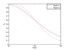
Figure 2. Graphs of $C(0,100,i)$ (panel a) and $\phi_{0}(i)$ (panel b) for $i\in\{1,2\}$ and for strikes in $[50,150]$.

Remark 5.1.

A clear advantage of our methodology over the one proposed by Shen et al., (2014) is that we have an interesting justification for the choice of the equivalent martingale measure. Furthermore, our methodology is easy to implement for any number of underlying assets while a discretization used to compute inverse Fourier transforms will be almost impossible to implement for more than three assets.

5.2. Second example

Next, we consider the log-returns of the stock price of Apple (aapl), from January 2nd, 2010 to April 24th, 2015. In order to estimate the parameters of the model, we first fit a regime-switching Gaussian random walk model on the returns, following the methodology proposed in Rémillard, (2013, Chapter 10). In this case, one has a discrete time Markov chain for the regimes, instead of a continuous time one. Also, given a regime $i$ at period $t$, the return at this period is Gaussian with a mean and variance depending on the regime. It is easy to check that the continuous time limit in this case is a regime-switching Brownian motion. According to Rémillard, (2013) and Rémillard et al., (2014), the appropriate number of regimes should be the first number so that one does not reject the null hypothesis of a Gaussian regime-switching. In the present case, the P-value for only one regime is 0%, while the P-value is $8\%$ for two regimes (using 1000 bootstrap samples). The estimated parameters are given in Tables 3, while the transition matrix is $Q=\left(\begin{array}[]{cc}0.7600&0.2400\\ 0.0590&0.9410\end{array}\right)$.

Table 3. Parameters estimation for the two-regime model on Apple daily returns from 01/02/2010 to 04/23/2015.

Regime	Mean	Volatility	Stat. distr.	Prob. of regime at current time
1	-0.0018	0.0283	0.1973	0.0441
2	0.0018	0.0123	0.8027	0.9559

To obtain the associated parameters of a RSGBM on an annual time scale, one can solve $Q=\exp\{\Lambda/252\}$. Here, one gets $\Lambda=\left(\begin{array}[]{cc}-71.8620&\phantom{-}71.8620\\ \phantom{-}17.6661&-17.6661\end{array}\right)$.

Remark 5.2.

Solving $Q=\exp\{\Lambda/252\}$ is not always possible. In practice, $\Lambda\approx 252(Q-I)$ is used. However, the relationship $Q=\exp\{\Lambda/252\}$ no longer holds and their could be discrepancies for option values in the discrete and continuous cases.

To find the remaining parameters in continuous time (measured in years), one can use the fact that for regime $i$, the mean of the regime-switching random walk is approximately $(\mu_{i}-\sigma_{i}^{2}/2)/252$, while its variance is approximately $\sigma_{i}^{2}/252$. The resulting parameters are given in Table 4. One can then interpret regime 1 as a “bad” regime, since $\mu_{1}<0$ is negative and $\sigma_{1}$ is twice the value in regime 2, and $\mu_{2}>0$. Fortunately, it follows from the stationary distribution that the “good” regime appears 80% of the time. Also, there is a 95.5% chance that the current regime on April 24th, 2015, is the good one. Finally, the estimated (annual) volatility is $.2658$, and the annual rate, based on the 1-month Libor, is 2.16%.

Table 4. Parameters for the RSGBM.

Regime	$\mu$	$\sigma$
1	-0.3436	0.4486
2	0.4813	0.1945

In order to compare some models, one will use the values of Table 5, giving the bid/ask of call options on Apple, expiring at $T=20/252$, for three strike prices. As one can see from Table 5, the Black-Scholes model under-estimate the market values.

Table 5. Market values, Black-Scholes price (BS) and delta-hedging value ($\phi_{0}$) for a call on Apple, as of April 24th 2015. The maturity day is May 22nd 2015 and the observed stock value is $129.95$.

Strike	Bid	Ask	BS	$\phi_{0}$
$128$	$5.50$	$5.65$	$5.0304$	$0.6034$
$129$	$4.95$	$5.10$	$4.4776$	$0.5629$
$130$	$4.45$	$4.50$	$3.9658$	$0.5220$

Next, as a first approximation, we can compute the call option prices and initial investment values using the semi-exact method for optimal discrete time hedging, as described in Chapter 3 of Rémillard, (2013). See also Rémillard and Rubenthaler, (2013). The values corresponding to a daily hedging are given in Table 6. It is worth noting that the Black-Scholes prices are larger than the regime 2 prices, and smaller than the regime 1 values.

Table 6. Call option prices and initial investment values using the semi-exact method optimal hedging method as in Chapter 3 of Rémillard, (2013). The number of hedging periods is 20 and the grid is composed of 2000 equidistant points in the interval $[50,200]$.

	Call value		Initial value $\phi_{0}$
Strike	Regime 1	Regime 2	Regime 1	Regime 2
$128$	$5.3981$	$4.9069$	$0.5951$	$0.6166$
$129$	$4.8430$	$4.3385$	$0.5578$	$0.5748$
$130$	$4.3268$	$3.8141$	$0.5202$	$0.5321$

Finally, we can find the option values provided by the optimal hedging for the RSGBM. Since the interest rate is not assumed to depend on the regime in this example, one gets $\tilde{\Lambda}=\stackrel{{\scriptstyle\circ}}{{\Lambda}}$. Its graph is displayed in Figure 3. From it, one see that one can take $\lambda=72.2522$. The 95% confidence intervals for the call value and the initial number of shares $\phi_{0}$, based on $10^{6}$ simulations of $\tilde{S}_{T}$, are given in Table 7. The resulting values for strike prices ranging from $125$ to $150$ are displayed in Figure 4. Comparing Tables 6 and 7, it seems that as the number of hedging periods tends to infinity, the option value under regime 1 decreases while it increases under regime 2. Also, the Black-Scholes values appear significantly larger than those of regime 1 and regime 2.

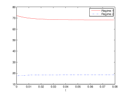
Figure 3. Graph of $-\left(\tilde{\Lambda}_{t}\right)_{ii}$ for $i\in\{1,2\}$ and $t\in[0,1/12]$.

Table 7. Call option prices and initial investment values computed by Monte Carlo with $10^{6}$ simulations, using antithetic variables.

	Call value		Initial value $\phi_{0}$
Strike	Regime 1	Regime 2	Regime 1	Regime 2
$128$	$5.0210\pm 0.0094$	$4.9813\pm 0.0094$	$0.6070\pm 0.0007$	$0.6092\pm 0.0007$
$129$	$4.4653\pm 0.0090$	$4.4236\pm 0.0090$	$0.5648\pm 0.0007$	$0.5659\pm 0.0007$
$130$	$3.9523\pm 0.0085$	$3.9097\pm 0.0085$	$0.5222\pm 0.0007$	$0.5222\pm 0.0007$

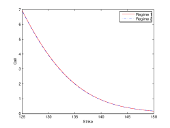
(a) (b)

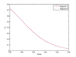
Figure 4. Graphs of $C(0,100,i)$ (panel a) and $\phi_{0}(i)$ (panel b) for $i\in\{1,2\}$ and for strike values in $[125,150]$.

Note that under-estimating the option value is not necessarily a bad thing. As proposed in Rémillard, (2013), since the market values are all larger, one could short the call option, invest $C_{0}$ (as computed in Table 7) in a portfolio based on optimal hedging for the RSGBM model, and invest the remaining value in a risk-free account. If transactions fees were negligible, one could make on average the difference between the initial option prices. This was tested on real data in Rémillard et al., (2014).

6. Conclusion

In this paper we presented the variance-optimal equivalent martingale measure $\tilde{P}$ and we found the optimal hedging solution for pricing and hedging an option under a regime-switching geometric Brownian motion model, extending the Black-Scholes model. The option price and the optimal strategy can be deduced from $\tilde{P}$, whose law is easy to simulate. Compared to some existing methods relying on inverse Fourier transforms, the proposed methodology has the advantage that it is easy to implement for any number of underlying assets.

Appendix A Construction of inhomogeneous Markov chains

Suppose that the (inhomogeneous) Markov chain $\tau_{t}$ has infinitesimal generator $\Lambda_{t}$, i.e., for any $j\neq i$, $\displaystyle\lim_{h\downarrow 0}\frac{1}{h}P(\tau_{t+h}=j|\tau_{t}=i)=(\Lambda_{t})_{ij}$. For a given $T$, assume that one can find $0<\lambda$ so that $-(\Lambda_{t})_{ii}\leq\lambda$, for any $i\in\{1,\ldots,l\}$ and any $t\in[0,T]$.

Algorithm 1.

To construct the Markov chain $\tau$, do the following:

• Generate $N\sim{\rm Poisson}(\lambda T)$.

• If $N=n$, generate independent uniform variates $U_{1},\ldots,U_{n}$ and order them. Denote the resulting sample by $U_{n:1},\ldots,U_{n:n}$, with $U_{n:1}<U_{n:2}\cdots<U_{n:n}$. This can be done by generating $n+1$ independent exponential variates $E_{1},\ldots,E_{n+1}$ and by setting $U_{n:i}=\frac{\sum_{j=1}^{i}E_{j}}{\sum_{j=1}^{n+1}E_{j}}$, $i\in\{1,\ldots,n\}$.

• Set $t_{i}=T\times U_{n:i}$, $i=1,\ldots,n$. These values are the possible transition times. Further set $t_{0}=0$ and $t_{n+1}=T$.

• For $k=1,\ldots,n$, if $\tau_{t_{k-1}}=i$, then $\tau_{t_{k}}=j$ with probability $P_{k,ij}$, where $P_{k,ij}=(\Lambda_{t_{k}})_{ij}/\lambda$ for $j\neq i$, and $P_{k,ii}=1+(\Lambda_{t_{k}})_{ii}/\lambda$.

A.1. Proof of Proposition 3.7

To show that the density of $S_{t}$ is infinitely differentiable with respect to $s$ and $t$, we use Algorithm 1, together with representation (2.2). Conditional on $N_{t}=n$ and $\mathcal{F}_{T}^{\tau}$, the returns $R_{t}^{(i)}=\log\left(S_{t}^{(i)}/s^{(i)}\right)$, $i\in\{1,\ldots,d\}$, are Gaussian, with mean $tV_{t}$, with $V_{t}=\frac{1}{t}\int_{0}^{t}v_{\tau_{u}}du$ and covariance matrix $tA_{t}$, with $A_{t}=\frac{1}{t}\int_{0}^{t}a_{\tau_{u}}du$, where $V_{t}=\sum_{k=1}^{n}\left(U_{n:k}-U_{n:k-1}\right)v(\tau_{t_{k-1}})+\left(1-U_{n:n}\right)v(\tau_{t_{n}})$ and $A_{t}=\sum_{k=1}^{n}\left(U_{n:k}-U_{n:k-1}\right)a(\tau_{t_{k-1}})+(1-U_{n:n})a(\tau_{t_{n}})$. Here, $U_{n:0}=0$. Next, set if $\alpha_{0}=i$ and $u_{0}=0$. Then, for any bounded measurable functions $\phi,\psi$, given $N_{t}=n$, one gets

$$E\{\phi(V_{t})\psi(A_{t})\} = n!\sum_{\alpha_{1}=1}^{l}\cdots\sum_{\alpha_{n}=1}^{l}\int_{0<u_{1}<\cdots<u_{n}<1}\prod_{k=1}^{n}g_{\alpha_{k-1}\alpha_{k}}\left(\frac{\Lambda_{tu_{k}}}{\lambda}\right)$$

$$\quad\times\phi\left\{\sum_{k=1}^{n}(u_{k}-u_{k-1})v(\alpha_{k-1})+(1-u_{n})v(\alpha_{n})\right\}$$

$$\qquad\times\psi\left\{\sum_{k=1}^{n}(u_{k}-u_{k-1})a(\alpha_{k-1})+(1-u_{n})a(\alpha_{n})\right\}du_{1}\cdots du_{n},$$

where $g_{ij}(x)=x_{ij}$ when $j\neq i$, and $g_{ii}(x)=1+x_{ii}$, $i\in\{1,\ldots,l\}$. Hence, if $\Lambda$ is continuously differentiable with respect to $t$, then it follows that the density of $S_{t}$ is infinitely differentiable with respect to $s$, as well as continuously differentiable with respect to $t$. Moreover these derivatives are all integrable. ∎

Appendix B Auxiliary results

Theorem B.1 (Feynman-Kac formula).

Let $\tau$ be a continuous Markov chain on $\{1,\ldots,l\}$, with infinitesimal generator $\Lambda$, and suppose that $f,V\in\mathbb{R}^{l}$. Then

$$u_{t}(i)=E_{i}\left[f(\tau_{t})e^{\int_{0}^{t}V(\tau_{u})du}\right],\quad i\in\{1,\ldots,l\},$$ (B.1)

is the unique solution of

$$\dot{u}_{t}(i)=\partial_{t}u_{t}(i)=(\Lambda u_{t})(i)+V(i)u_{t}(i),\quad u_{0}(i)=f(i).$$ (B.2)

Proof.

First, $u$ exists and is unique since (B.2) is a system of finite linear ode’s. In fact, $u_{t}=e^{t\{\Lambda+D(v)\}}f$. Next, let $u$ be defined by (B.1). Then, $u$ is bounded, $u_{0}=f$, and for any $h\geq 0$, since $\tau$ is Markov, $u_{t+h}(i)=E_{i}\left[u_{t}(\tau_{h})e^{\int_{0}^{h}V(\tau_{s})ds}\right]$, $i\in\{1,\ldots,l\}$. Next, if $\zeta=\inf\{s>0;\tau_{s}\neq i\}$, then $P_{i}(\zeta>s)=e^{s\Lambda_{ii}}$ and the event that there are at least two state changes in the time interval $[0,h]$ is $o(h)$. As a result,

$$u_{t+h}(i) = \left(1+\Lambda_{ii}h+o(h)\right)u_{t}(i)e^{hV(i)}+\sum_{j\neq i}\Lambda_{ij}u_{t}(j)\int_{0}^{h}e^{s\Lambda_{ii}}e^{sV(i)+(h-s)V(j)}ds+o(h)$$

$$= u_{t}(i)+hV(i)u_{t}(i)+h(\Lambda u_{t})_{i}+o(h).$$

Hence, $u$ satisfies (B.2). ∎

B.1. Proof of Lemma 3.1

Let $i\in\{1,\ldots,l\}$ be given. We only prove the statements for $\gamma$. First, by the uniqueness of (3.3) and the Feynman-Kac formula in Theorem B.1, one obtains that for any $i\in\{1,\ldots,l\}$, $\gamma_{i}(t)=E_{i}\left\{e^{-\int_{0}^{t}\ell_{\tau_{u}}du}\right\}$, so $\gamma_{i}(t)\leq 1$ and $\gamma_{i}(t)>0$. Next, $\frac{d}{dt}\left\{\gamma_{i}(t)e^{(\ell_{i}-\Lambda_{ii})t}\right\}=e^{(\ell_{i}-\Lambda_{ii})t}\sum_{j\neq i}\Lambda_{ij}\gamma_{j}(t)$. As a result, for all $t\geq 0$ $\frac{d}{dt}\left\{\gamma_{i}(t)e^{(\ell_{i}-\Lambda_{ii})t}\right\}\geq 0$, so $\gamma_{i}(t)\geq e^{(\Lambda_{ii}-\ell_{i})t}$. ∎

Lemma B.2.

Let $(x_{t})$ be a Markov process in $\mathbb{R}^{l}$ with infinitesimal generator $\mathcal{L}$ and set $\mathcal{L}_{t}f_{t}=\partial_{t}f_{t}+\mathcal{L}f_{t}$. Suppose that $M_{t}^{(f)}=f_{t}(x_{t})-f_{0}(x_{0})-\int_{0}^{t}\mathcal{L}_{u}f_{u}(x_{u})du$, $M_{t}^{(g)}=g_{t}(x_{t})-g_{0}(x_{0})-\int_{0}^{t}\mathcal{L}_{u}g_{u}(x_{u})du$, $M_{t}^{(fg)}=f_{t}(x_{t})g_{t}(x_{t})-f_{0}(x_{0})g_{0}(x_{0})-\int_{0}^{t}\mathcal{L}_{u}(f_{u}g_{u})(x_{u})du$ are martingales. Then, $M_{t}^{(f,g)}=M_{t}^{(f_{u}g_{u})}-\int_{0}^{t}g_{u}(x_{u})dM_{u}^{(f)}-\int_{0}^{t}f_{u}(x_{u})dM_{u}^{(g)}$ is a martingale and $M_{t}^{(f,g)}=\left[M^{(f)},M^{(g)}\right]_{t}-\int_{0}^{t}\{\mathcal{L}_{u}(f_{u}g_{u})-f_{u}\mathcal{L}_{u}g_{u}-g_{u}\mathcal{L}_{u}f_{u}\}(x_{u})du$.

Proof.

By definition, $M_{t}^{(f)}M_{t}^{(g)}=\int_{0}^{t}M_{u}^{(f)}dM_{u}^{(g)}+\int_{0}^{t}M_{u}^{(g)}dM_{u}^{(f)}+\left[M^{(f)},M^{(g)}\right]_{t}$. Setting $V^{(f)}_{t}=\int_{0}^{t}\mathcal{L}_{u}f_{u}(x_{u})du$ and $V^{(g)}_{t}=\int_{0}^{t}\mathcal{L}_{u}g_{u}(x_{u})du$, one gets $M_{t}^{(f)}V^{(g)}_{t}=\int_{0}^{t}\mathcal{L}_{u}g_{u}(x_{u})M_{u}^{(f)}du+\int_{0}^{t}V^{(g)}_{u}dM_{u}^{(f)}$, and $M_{t}^{(g)}V^{(f)}_{t}=\int_{0}^{t}\mathcal{L}_{u}f_{u}(x_{u})M_{u}^{(g)}du+\int_{0}^{t}V^{(f)}_{u}dM_{u}^{(g)}$. Next, one obtains

$$M_{t}^{(f,g)} = M_{t}^{(fg)}-\int_{0}^{t}g_{u}(x_{u})dM_{u}^{(f)}-\int_{0}^{t}f_{u}(x_{u})dM_{u}^{(g)}$$

$$= f_{t}(x_{t})g_{t}(x_{t})-f_{0}(x_{0})g_{0}(x_{0})-\int_{0}^{t}\mathcal{L}_{u}(f_{u}g_{u})(x_{u})du$$

$$\qquad-\int_{0}^{t}g_{u}(x_{u})dM_{u}^{(f)}-\int_{0}^{t}f_{u}(x_{u})dM_{u}^{(g)}$$

$$= \left(M_{t}^{(f)}+V_{t}^{(f)}\right)\left(M_{t}^{(g)}+V_{t}^{(g)}\right)+f_{0}(x_{0})V_{t}^{(g)}+g_{0}(x_{0})V_{t}^{(f)}$$

$$\qquad-\int_{0}^{t}\{g_{u}(x_{u})-g_{0}(x_{0})\}dM_{u}^{(f)}-\int_{0}^{t}\{f_{u}(x_{u})-f_{0}(x_{0})\}dM_{u}^{(g)}$$

$$\qquad\qquad-\int_{0}^{t}\mathcal{L}_{u}(f_{u}g_{u})(x_{u})du$$

$$= \left(M_{t}^{(f)}+V_{t}^{(f)}\right)\left(M_{t}^{(g)}+V_{t}^{(g)}\right)+f_{0}(x_{0})V_{t}^{(g)}+g_{0}(x_{0})V_{t}^{(f)}$$

$$\qquad-\int_{0}^{t}\left(M_{u}^{(g)}+V_{u}^{(g)}\right)dM_{u}^{(f)}-\int_{0}^{t}\left(M_{u}^{(f)}+V_{u}^{(f)}\right)dM_{u}^{(g)}$$

$$\qquad\qquad-\int_{0}^{t}\mathcal{L}_{u}(f_{u}g_{u})(x_{u})du$$

$$= [M^{(f)},M^{(g)}]_{t}-\int_{0}^{t}\{\mathcal{L}_{u}(f_{u}g_{u})-f_{u}\mathcal{L}_{u}g_{u}-g_{u}\mathcal{L}_{u}f_{u}\}(x_{u})du.$$

Hence the result. ∎

Note that if $g(s)=s$, then for any smooth function $f$,

$$\left\{\mathcal{L}_{i}(fg)-f\mathcal{L}_{i}g-g\mathcal{L}_{i}f\right\}(s,i)=D(s)a(i)D(s)\nabla f(s,i).$$ (B.3)

Appendix C Proof of the main results

C.1. Proof of Lemma 3.3

The multiplicative character of $Z$ follows directly from the representation $Z_{t}=e^{-M_{t}-\frac{1}{2}\int_{0}^{t}\ell_{\tau_{u}}du}$, $M_{t}=\int_{0}^{t}\ell_{\tau_{u}}du+\int_{0}^{t}\rho(\tau_{u-})^{\top}\sigma(\tau_{u-})dW_{u}$, since $\tau$ and $(W,\tau)$ are Markov processes. Hence, for any $s,t\geq 0$, $Z_{t+s}=Z_{t}Z_{t,s}$ where for a fixed $t$, $Z_{t,s}$ is independent of $\mathcal{F}_{t}$ and has the same law as $Z_{s}$. Next, from Lemma 3.1, $Z^{(2)}$ is a positive martingale. Next, since $W$ and $\tau$ are independent and $\mathcal{F}_{t}=\mathcal{F}_{t}^{W}\vee\mathcal{F}_{t}^{\tau}\subset\mathcal{F}_{t}^{W}\vee\mathcal{F}_{T}^{\tau}$, it follows that for any $t\in[0,T]$,

$$E[Z_{T}|\mathcal{F}_{t}] = E\left[Z_{T}^{(1)}Z_{T}^{(2)}|\mathcal{F}_{t}\right]=E\left[Z_{T}^{(2)}E\left[Z_{T}^{(1)}|\mathcal{F}_{t}^{W}\vee\mathcal{F}_{T}^{\tau}\right]|\mathcal{F}_{t}\right]$$

$$= E\left[Z_{t}^{(1)}Z_{T}^{(2)}|\mathcal{F}_{t}\right]=Z_{t}^{(1)}E\left[Z_{T}^{(2)}|\mathcal{F}_{t}\right]=Z_{t}^{(1)}Z_{t}^{(2)}=Z_{t}\gamma_{\tau_{t}}(T-t),$$

proving that $Z_{t}^{(1)}Z_{t}^{(2)}$ is a martingale for $t\in[0,T]$. Similarly, from Lemma 3.1,

$$E_{i}(Z_{t})=E_{i}\left[e^{-\int_{0}^{t}\ell_{\tau_{u}}du}E\left[Z_{t}^{(1)}|\mathcal{F}_{t}^{\tau}\right]\right]=E_{i}\left[e^{-\int_{0}^{t}\ell_{\tau_{u}}du}\right]=\gamma_{i}(t),\quad t\geq 0.$$

Now take $\theta\in\mathbb{R}^{d}$, $f\in\mathbb{R}^{l}$, and let $0\leq s\leq t\leq T$ be given. Then

$$E^{\tilde{P}}\left[f(\tau_{t})e^{\theta^{\top}(\tilde{W}_{t}-\tilde{W}_{s})}|\mathcal{F}_{s}\right] = E\left[Z_{t}^{(1)}Z_{t}^{(2)}f(\tau_{t})e^{\theta^{\top}(\tilde{W}_{t}-\tilde{W}_{s})}|\mathcal{F}_{s}\right]/(Z_{s}^{(1)}Z_{s}^{(2)})$$

$$= E\left[Z_{t}^{(2)}f(\tau_{t})E\left[Z_{t}^{(1)}e^{\theta^{\top}(\tilde{W}_{t}-\tilde{W}_{s})}|\mathcal{F}_{s}^{W}\vee\mathcal{F}_{t}^{\tau}\right]|\mathcal{F}_{s}\right]/(Z_{s}^{(1)}Z_{s}^{(2)}).$$

Now, set $h_{u}=\sigma_{\tau_{u}}^{\top}\rho_{\tau_{u}}$. Novikov’s condition is clearly satisfied for $h$ and one can check that

$$E\left[Z_{t}^{(1)}e^{\theta^{\top}\tilde{W}_{t}}|\mathcal{F}_{s}^{W}\vee\mathcal{F}_{t}^{\tau}\right]=e^{\|\theta\|^{2}(t-s)}Z_{s}^{(1)}e^{\theta^{\top}\tilde{W}_{s}}.$$

Hence

$$E^{\tilde{P}}\left[f(\tau_{t})e^{\theta^{\top}(\tilde{W}_{t}-\tilde{W}_{s})}|\mathcal{F}_{s}\right] = e^{\|\theta\|^{2}(t-s)}E\left[Z_{t}^{(2)}f(\tau_{t})\right]/Z_{s}^{(2)}$$

$$= e^{\|\theta\|^{2}(t-s)}E\left[\gamma_{\tau_{t}}(T-t)e^{-\int_{s}^{t}\ell_{\tau_{u}}du}f(\tau_{t})\right]/\gamma_{\tau_{s}}(T-s)$$

$$= e^{\|\theta\|^{2}(t-s)}E_{\tau_{s}}\left[\gamma_{\tau_{t-s}}(T-t)e^{-\int_{0}^{t-s}\ell_{\tau_{u}}du}f(\tau_{t-s})\right]/\gamma_{\tau_{s}}(T-s).$$

This proves that under $\tilde{P}$, $\tilde{W}$ is a Brownian motion independent of $\tau$, and consequently,

$$X_{t} = X_{0}+\int_{0}^{t}D(X_{u})m_{\tau_{u}}du+\int_{0}^{t}D(X_{u})\sigma_{\tau_{u-}}dW_{u}$$

$$= X_{0}+\int_{0}^{t}D(X_{u})\left(m_{\tau_{u}}-\sigma_{\tau_{u}}\sigma_{\tau_{u}}^{\top}\rho_{\tau_{u}}\right)du+\int_{0}^{t}D(X_{u})\sigma_{\tau_{u-}}d\tilde{W}_{u}$$

$$= X_{0}+\int_{0}^{t}D(X_{u})\sigma_{\tau_{u-}}d\tilde{W}_{u},$$

proving that $X$ is a $\tilde{P}$-martingale. Similarly, $S_{t}=S_{0}+\int_{0}^{t}r_{\tau_{u}}S_{u}du+\int_{0}^{t}D(S_{u})\sigma_{\tau_{u-}}d\tilde{W}_{u}$. Finally, if $0\leq t\leq t+h\leq T$, then

$$E^{\tilde{P}}\left[f(\tau_{t+h})|\mathcal{F}_{t}\right] = E_{\tau_{t}}\left[\gamma_{\tau_{h}}(T-t-h)e^{-\int_{0}^{h}\ell_{\tau_{u}}du}f(\tau_{h})\right]/\gamma_{\tau_{t}}(T-t)$$

$$= E_{\tau_{t}}\left[\gamma_{\tau_{h}}(T-t)e^{-\int_{0}^{h}\ell_{\tau_{u}}du}f(\tau_{h})\right]/\gamma_{\tau_{t}}(T-t)$$

$$\quad-hE_{\tau_{t}}\left[\dot{\gamma}_{\tau_{h}}(T-t)e^{-\int_{0}^{h}\ell_{\tau_{u}}du}f(\tau_{h})\right]/\gamma_{\tau_{t}}(T-t)+o(h).$$

It follows from Theorem B.1 that if $v_{h}(i)=E_{i}\left[\gamma_{\tau_{h}}(T-t)e^{-\int_{0}^{h}\ell_{\tau_{u}}du}f(\tau_{h})\right]$, then

$$v_{h}(i) = \gamma_{i}(T-t)f(i)+h\sum_{j=1}^{l}\Lambda_{ij}\gamma_{j}(T-t)f(j)-h\ell_{i}\gamma_{i}(T-t)f(i)+o(h)$$

$$= \gamma_{i}(T-t)f(i)+h\gamma_{i}(T-t)\sum_{j=1}^{l}\left({\tilde{\Lambda}}_{T-t}\right)_{ij}f(j)$$

$$\qquad+h\gamma_{i}(T-t)f(i)\left\{\Lambda_{ii}-\left({\tilde{\Lambda}}_{T-t}\right)_{ii}-\ell_{i}\right\}+o(h)$$

$$= \gamma_{i}(T-t)f(i)+h\gamma_{i}(T-t)\sum_{j=1}^{l}\left({\tilde{\Lambda}}_{T-t}\right)_{ij}f(j)+h\dot{\gamma}_{i}(T-t)f(i)+o(h),$$

using $\dot{\gamma}_{i}(t)=-\ell_{i}\gamma_{i}(t)+\Lambda_{ii}\gamma_{i}(t)-(\tilde{\Lambda}_{t})_{ii}\gamma_{i}(t)$, from (3.7). Therefore, if $\tau_{t}=i$, then

$$E^{\tilde{P}}\left[f(\tau_{t+h})|\mathcal{F}_{t}\right]=f(i)+h{\tilde{\Lambda}}_{T-t}f(i)+o(h),$$

showing that under $\tilde{P}$, $\tau$ is a Markov chain with generator ${\tilde{\Lambda}}_{T-t}$. ∎

C.2. Proof of Lemma 3.5

To prove that $\tilde{P}$ is variance-optimal, set $b_{t}=D^{-1}(X_{t})\rho(\tau_{t-})$, so that $M_{t}=\int_{0}^{t}b_{u}^{\top}dX_{u}$. It is then easy to check that $\bar{b}=bZ$ is such that $\int_{0}^{T}\bar{b}_{u}^{\top}dX_{u}$ is square integrable, and since $X$ is a $\tilde{P}$-martingale, then for any bounded stopping times $U,V$ with $0\leq U\leq V\leq T$, and any bounded $\mathcal{F}_{U}$-measurable variable $H$, one gets $E\left[Z_{T}H(X_{V}-X_{U})\right]=0$, proving that $b$ is an adjustment process, as defined in Schweizer, (1996). It follows from Schweizer, (1996, Proposition 8) that $\tilde{P}$ is variance-optimal. ∎

C.3. Proof of Lemma 3.11

If $f(s,i)$ is twice continuously differentiable with respect to $s$ and $(S_{t},{\tau}_{t})=(s,i)$, then

$$E^{\check{P}}\left[f(S_{t+h},\tau_{t+h})|\mathcal{F}_{t}\right] = \frac{\beta_{i}(T-t)}{s}E^{\stackrel{{\scriptstyle\circ}}{{P}}}\left[S_{T}f(S_{t+h},\tau_{t+h})|\mathcal{F}_{t}\right]$$

$$= \frac{\beta_{i}(T-t)}{s}\frac{E^{\tilde{P}}\left[B_{T}S_{T}f(S_{t+h},\tau_{t+h})|\mathcal{F}_{t}\right]}{E^{\tilde{P}}\left[B_{T}|\mathcal{F}_{t}\right]}$$

$$= \frac{1}{sB_{t}}E^{\tilde{P}}\left[X_{T}f(S_{t+h},\tau_{t+h})|\mathcal{F}_{t}\right]=\frac{1}{sB_{t}}E^{\tilde{P}}\left[X_{t+h}f(S_{t+h},\tau_{t+h})|\mathcal{F}_{t}\right].$$

Then, with $g$ being the identity function, if $(S_{t},{\tau}_{t})=(s,i)$, it follows that

$$\lim_{h\downarrow 0}\frac{1}{h}\left[E^{\check{P}}\left[f(S_{t+h},\tau_{t+h})|\mathcal{F}_{t}\right]-f(s,i)\right] = -r_{i}f(s,i)+\frac{\tilde{\mathcal{H}}_{t}(fg)(s,i)}{s}=\check{\mathcal{H}}_{t}f(s,i).$$

∎

C.4. Proof of Lemma 4.1

According to Protter, (2004)[Theorem V.7], the solution of $V_{t}=C_{0}(s,i)+\int_{0}^{t}\alpha_{u}(S_{u},\tau_{u-})^{\top}dX_{u}-\int_{0}^{t}V_{u-}dM_{u}$ exists and is uniquely determined by $M$ and $S$. See also Remark C.1 below. Next, $\phi_{t}=\alpha_{t}(S_{t-},\tau_{t-})-V_{t-}D^{-1}(X_{t-})\rho(\tau_{t-})$, so $\phi$ is predictable and $V_{t}=C_{0}(s,i)+\int_{0}^{t}\phi_{u}^{\top}dX_{u}$, by definition of $M$. ∎

Remark C.1.

Since the martingale $M$ is continuous, Protter, (2004)[Theorem V.52] yields the representation $V_{t}=Z_{t}\left\{H_{0}+\int_{0+}^{t}Z_{u}^{-1}d(H_{u}+[H,M]_{u})\right\}$, where

$$H_{t} = C_{0}(s,i)+\int_{0}^{t}\alpha_{u}(S_{u},\tau_{u-})^{\top}dX_{u}$$

$$= C_{0}(s,i)+\int_{0}^{t}\alpha_{u}(S_{u},\tau_{u-})^{\top}D(X_{u})m(\tau_{u})du$$

$$\quad+\int_{0}^{t}\alpha_{u}(S_{u},\tau_{u-})^{\top}D(X_{u})\sigma(\tau_{u-})dW_{u},$$

and $[H,M]_{t}=\int_{0}^{t}\alpha_{u}(S_{u},\tau_{u})^{\top}D(X_{u})m(\tau_{u})du$. As a result,

$$\frac{V_{t}}{Z_{t}} = C_{0}+2\int_{0}^{t}\frac{\alpha_{u}(S_{u},\tau_{u})^{\top}D(X_{u})m(\tau_{u})}{Z_{u}}du+\int_{0}^{t}\frac{\alpha_{u}(S_{u},\tau_{u})^{\top}D(X_{u})\sigma(\tau_{u})}{Z_{u}}dW_{u}.$$

C.5. Proof of Lemma 4.3

Let $M^{(C)}$ and $M^{(g)}$ be the martingales defined by $M_{t}^{(C)}=C_{t}(S_{t},\tau_{t})-C_{0}(s,i)-\int_{0}^{t}\left\{\partial_{u}C_{u}(S_{u},\tau_{u})+\mathcal{H}C_{u}(S_{u},\tau_{u})\right\}du$ and $M_{t}^{(g)}=S_{t}-s-\int_{0}^{t}D(S_{u})\mu(\tau_{u})du=\int_{0}^{t}D(S_{u})\sigma(\tau_{u-})dW_{u}$, with $g(s)=s$ on $[0,\infty)^{d}$. As a result, $X_{t}=s+\int_{0}^{t}D(X_{u})m(\tau_{u})du+\int_{0}^{t}B_{u}dM_{u}^{(g)}$,

$$V_{t} = C_{0}(s,i)+\int_{0}^{t}B_{u}\phi_{u}(S_{u-},\tau_{u-})^{\top}dM_{u}^{(g)}$$

$$\quad+\int_{0}^{t}B_{u}m(\tau_{u})^{\top}D(S_{u})\phi_{u}(S_{u},\tau_{u})du$$

$$= C_{0}(s,i)+\int_{0}^{t}B_{u}\phi_{u}(S_{u-},\tau_{u-})^{\top}dM_{u}^{(g)}$$

$$\quad+\int_{0}^{t}B_{u}m(\tau_{u})^{\top}D(S_{u})\nabla C_{u}(S_{u},\tau_{u})du+\int_{0}^{t}G_{u}\ell_{\tau_{u}}du$$

$$B_{t}C_{t}(S_{t},\tau_{t}) = C_{0}(s,i)+\int_{0}^{t}B_{u}\left\{\partial_{u}C_{(}S_{u},\tau_{u})-rC_{u}(S_{u},\tau_{u})\right\}du$$

$$\quad+\int_{0}^{t}B_{u}\mathcal{H}C_{u}(S_{u},\tau_{u})du+\int_{0}^{t}B_{u}dM_{u}^{(C)}.$$

Therefore, using (3.20) and using (4.4) one obtains that

$$G_{t} = -\int_{0}^{t}B_{u}{\tilde{\mathcal{H}}}_{T-u}C_{u}(S_{u},\tau_{u})du+\int_{0}^{t}B_{u}\mathcal{H}C_{u}(S_{u},\tau_{u})du+\int_{0}^{t}B_{u}dM_{u}^{(C)}$$ (C.1)

$$\quad-\int_{0}^{t}B_{u}m(\tau_{u})^{\top}D(S_{u})\nabla C_{u}(S_{u},\tau_{u})du-\int_{0}^{t}B_{u}\phi_{u}(S_{u},\tau_{u})^{\top}dM_{u}^{(g)}$$

$$\qquad-\int_{0}^{t}\ell_{\tau_{u}}G_{u}du$$

$$= \int_{0}^{t}B_{u}dM_{u}^{(C)}-\int_{0}^{t}B_{u}\phi_{u}(S_{u},\tau_{u})^{\top}dM_{u}^{(g)}-\int_{0}^{t}\ell_{\tau_{u}}G_{u}du$$

$$\quad+\int_{0}^{t}B_{u}\left\{(\Lambda-\tilde{\Lambda}_{T-u})C_{u,S_{u}}\right\}(\tau_{u})du.$$

Finally, it follows from Ito’s formula that

$$M_{t}^{(C)} = \int_{0}^{t}\nabla_{s}C_{u}(S_{u},\tau_{u})^{\top}D(S_{u})\sigma(\tau_{u-})dW_{u}$$

$$\qquad+\sum_{0<u\leq t}\Delta C_{u}(S_{u},\tau_{u})-\int_{0}^{t}\Lambda C_{u}(S_{u},\tau_{u})du.$$

Replacing in the above formula yields the desired result. ∎

C.6. Proof of Lemma 4.4

Let $g(s)=s$ and let $M^{(g)}$ be as defined in the proof of Lemma 4.3. Then, using (C.1) and Itô’s formula, one gets, for any smooth $f$,

$$G_{t}f_{t}(S_{t},\tau_{t}) = \int_{0}^{t}f_{u}(S_{u-},\tau_{u-})dG_{u}+\int_{0}^{t}\partial_{u}f_{u}(S_{u},\tau_{u})G_{u}du$$

$$\quad+\int_{0}^{t}\mathcal{H}f_{u}(S_{u},\tau_{u})G_{u}du+\int_{0}^{t}G_{u-}dM_{u}^{(f)}+\left[G,M^{(f)}\right]_{t}$$

$$= \int_{0}^{t}B_{u}f_{u}(S_{u-},\tau_{u-})dM_{u}^{(C)}+\int_{0}^{t}G_{u-}dM_{u}^{(f)}+\left[G,M^{(f)}\right]_{t}$$

$$\quad-\int_{0}^{t}B_{u}f_{u}(S_{u-},\tau_{u-})\phi_{u}^{\top}dM_{u}^{(g)}$$

$$\qquad+\int_{0}^{t}B_{u}f_{u}(S_{u},\tau_{u})\left\{(\Lambda-\tilde{\Lambda}_{T-u})C_{u,S_{u}}\right\}(\tau_{u})du$$

$$\qquad+\int_{0}^{t}\left\{\mathcal{H}f_{u}(S_{u},\tau_{u})+\partial_{u}f_{u}(S_{u},\tau_{u})-f_{u}(S_{u},\tau_{u})\ell_{\tau_{u}}\right\}G_{u}du,$$

where $M_{t}^{(f)}=f_{t}(S_{t},\tau_{t})-f_{0}(s,i)-\int_{0}^{t}\partial_{u}f_{u}(S_{u},\tau_{u})du-\int_{0}^{t}\mathcal{H}f_{u}(S_{u},\tau_{u})du$ is a martingale and where, by (C.1) and Lemma B.2, one has

$$\left[G,M^{(f)}\right]_{t} = \int_{0}^{t}B_{u}d\left[M^{(C)},M^{(f)}\right]_{u}-\int_{0}^{t}B_{u}\phi_{u}^{\top}d\left[M^{(g)},M^{(f)}\right]_{u}$$

$$= \int_{0}^{t}B_{u}dM_{u}^{(C,f)}-\int_{0}^{t}B_{u}\phi_{u}^{\top}dM_{u}^{(f,g)}$$

$$\quad+\int_{0}^{t}B_{u}\{\mathcal{H}(f_{u}C_{u})-f_{u}\mathcal{H}(C_{u})-C_{u}\mathcal{H}(f_{u})\}(S_{u},\tau_{u})du$$

$$\qquad-\int_{0}^{t}B_{u}\phi_{u}^{\top}\{\mathcal{H}(f_{u}g)-f_{u}\mathcal{H}(g)-g\mathcal{H}(f_{u})\}(S_{u},\tau_{u})du.$$

As a result, if $f_{t}(s,i)=\gamma_{T-t}(i)$, then $\mathcal{H}f_{u}(s,i)+\partial_{u}f_{u}(s,i)-f_{u}(s,i)\ell_{i}\equiv 0$, and $\mathcal{N}(f_{u},g)(s,i)=\{\mathcal{H}(f_{u}g)-f_{u}\mathcal{H}(g)-g\mathcal{H}(f_{u})\}(s,i)\equiv 0$, using (B.3). Moreover

$$\mathcal{N}(f_{u},C_{u})(s,i) = \left\{\mathcal{H}(f_{u}C_{u})-f_{u}\mathcal{H}(C_{u})-C_{u}\mathcal{H}(f_{u})\right\}(s,i)$$

$$= -\gamma_{T-u}(i)\Lambda C_{u,s}(i)-C_{u,s}(i)\Lambda\gamma_{T-u}(i)+\Lambda(\gamma_{T-u}C_{u,s})(i)$$

$$= -f_{u}(s,i)\left\{(\Lambda-\tilde{\Lambda}_{T-u})C_{u,s}\right\}(i),$$

since $\Lambda(\gamma_{t}h)(i)-\gamma_{t}(i)\Lambda h(i)-h(i)\Lambda\gamma_{t}(i)=\gamma_{t}(i)(\tilde{\Lambda}_{t}-\Lambda)h(i)$, $i\in\{1,\ldots,l\}$. Hence $G_{t}\gamma_{\tau_{t}}(T-t)$ is a martingale with initial value $0$ and terminal value $G_{T}$, since $\gamma(0)=\mathbf{1}$. Thus, $E(G_{T})=0$. Next, take $f_{t}(s,i)=s_{k}\gamma_{T-t}(i)$, for a given $k\in\{1,\ldots,d\}$. Then

$$\mathcal{N}(f_{u},g)(s,i)=\{\mathcal{H}(f_{u}g)-f_{u}\mathcal{H}(g)-g\mathcal{H}(f_{u})\}(s,i)=f_{u}(s,i)D(s)a(i)e_{k}$$

by (B.3), with $(e_{k})_{j}=I_{jk}$. Also, $\mathcal{H}f_{u}(s,i)+\partial_{u}f_{u}(s,i)-f_{u}(s,i)\ell_{i}=f_{u}(s,i)\mu_{k}(i)$ and

$$\mathcal{N}(f_{u},C_{u})(s,i) = \left\{\mathcal{H}(f_{u}C_{u})-f_{u}\mathcal{H}(C_{u})-C_{u}\mathcal{H}(f_{u})\right\}(s,i)$$

$$= f_{u}(s,i)e_{k}^{\top}a(i)D(s)\nabla C_{u}(s,i)-f_{u}(s,i)\left\{(\Lambda-\tilde{\Lambda}_{T-u})C_{u,s}\right\}(i),$$

using the previous calculations. It follows that $R_{t}-A_{t}$ is a martingale, where

$$A_{t}=\int_{0}^{t}B_{u}\phi_{u}^{\top}\left\{\mathcal{N}(f_{u},C_{u})-\mathcal{N}(f_{u},g)\right\}(S_{u},\tau_{u})du\\ +\int_{0}^{t}B_{u}f_{u}(S_{u},\tau_{u})\left\{(\Lambda-\tilde{\Lambda}_{T-u})C_{u,S_{u}}\right\}(\tau_{u})du\\ +\int_{0}^{t}\left\{\mathcal{H}f_{u}(S_{u},\tau_{u})+\partial_{u}f_{u}(S_{u},\tau_{u})-f_{u}(S_{u},\tau_{u})\ell_{\tau_{u}}\right\}G_{u}du.$$

Using (4.4) and setting $R_{t}=f_{t}(S_{t},\tau_{t})G_{t}$, one gets that

$$A_{t} = \int_{0}^{t}\left[R_{u}\{m_{k}(\tau_{u})+r_{\tau_{u}}\}+f_{u}(S_{u},\tau_{u})e_{k}^{\top}a(\tau_{u})D(X_{u})\{\nabla C_{u}(S_{u},\tau_{u})-\phi_{u})\}\right]du$$

$$= \int_{0}^{t}\left[R_{u}\{m_{k}(\tau_{u})+r_{\tau_{u}}\}-R_{u}e_{k}^{\top}a(\tau_{u})\rho(\tau_{u})\right]du=\int_{0}^{t}r_{\tau_{u}}R_{u}du,$$

proving that $R_{t}-\int_{0}^{t}r_{\tau_{u}}R_{u}du$ is a martingale. Hence, so is $B_{t}R_{t}=X_{t}G_{t}\gamma_{T-t}(\tau_{t})$. Finally, to prove (4.8), note that $E(G_{T}|\mathcal{F}_{t})=\gamma_{\tau_{t}}(T-t)G_{t}$. Thus, for any stopping times $U,V$ with $0\leq U\leq V\leq T$,

$$E\{G_{T}(X_{V}-X_{U})|\mathcal{F}_{u}\} = E\{(X_{V}E(G_{T}|\mathcal{F}_{V})|\mathcal{F}_{U}\}-X_{U}E(G_{T}|\mathcal{F}_{U})$$

$$= E\{G_{V}\gamma_{\tau_{V}}(T-V)X_{V}-G_{U}\gamma_{\tau_{U}}(T-U)X_{U}|\mathcal{F}_{U}\}=0,$$

since we just proved that $X_{t}G_{t}\gamma_{\tau_{t}}(T-t)$ is a martingale. Hence the result.∎

C.7. Proof of Theorem 4.5

It follows from (4.8) that for any stopping times $U,V$, with $0\leq U\leq V\leq T$, and any bounded random variable $Y$ that is $\mathcal{F}_{U}$-measurable, $E\left(G_{T}\int_{0}^{T}\psi_{t}^{\top}dX_{t}\right)=0$, where $\psi$ is the predictable process given by $\psi_{t}=Y1_{(U,V]}(t)$. Therefore, using properties of stochastic integrals, one may conclude that for any admissible strategy $\psi$, one gets $E\left(G_{T}\int_{0}^{T}\psi_{t}^{\top}dX_{t}\right)=0$. Since $E\left\{G_{T}\int_{0}^{T}(\phi_{t}-\psi_{t})^{\top}dX_{t}\right\}=0$ and $E(G_{T})=0$, one has, for any $(\pi,\psi)\in\mathbb{R}\times\mathcal{A}$,

$$\mathit{HE}(\pi,\psi)=\mathit{HE}(C_{0},\phi)+E\left[\left\{C_{0}(s,i)-\pi+\int_{0}^{T}(\phi_{t}-\psi_{t})^{\top}dX_{t}\right\}^{2}\right]\geq\mathit{HE}(C_{0},\phi).$$

This proves that at least one solution exists. Suppose now that $\mathit{HE}(\pi,\psi)=\mathit{HE}(C_{0},\phi)$ for some $(\pi,\psi)\in\mathbb{R}\times\mathcal{A}$. Then $C_{0}(s,i)-\pi+\int_{0}^{T}(\phi_{t}-\psi_{t})^{\top}dX_{t}=0$ $P$ almost surely. Since $\tilde{P}$ is equivalent to $P$ and $X$ is a $\tilde{P}$-martingale, it follows that $N_{t}=\int_{0}^{t}(\phi_{s}-\psi_{s})^{\top}dX_{s}$ is a $\tilde{P}$-martingale. Hence its expectation is $0$, implying that so $C_{0}=\pi$. It then follows that $N_{t}\equiv 0$ $P$-a.s. Finally, the $\tilde{P}$-martingale $N$ has quadratic variation $[N,N]_{t}=\int_{0}^{t}\|\psi_{s}-\phi_{s}\|^{2}\ell_{\tau_{s}}ds$ for all $t\in[0,T]$. Now, $N_{t}^{2}-[N,N]_{t}$ is a martingale having expectation $0$. Since $N_{T}=0$ $\tilde{P}$-a.s., it follows that $[N,N]_{T}=0$ $\tilde{P}$-a.s., proving that for all almost every $t\in[0,T]$, $\psi_{t}=\phi_{t}$ a.s. under $P$ and $\tilde{P}$. This proves the uniqueness. ∎

Appendix D Laplace transforms of $\log(S_{T})$ under $\stackrel{{\scriptstyle\circ}}{{P}}$ and $\check{P}$

One can compute the Laplace transform or the characteristic function of the conditional distribution of $\log\left(S_{T}/s\right)$ given $S_{t}=s,{\tau}_{t}=i$ under $\stackrel{{\scriptstyle\circ}}{{P}}$ in the following way. Note that for any $0\leq t\leq T$, and for any $\theta\in\mathbb{C}$,

$$\stackrel{{\scriptstyle\circ}}{{\Psi}}_{T-t}(i,\theta)=E_{s,i}^{\stackrel{{\scriptstyle\circ}}{{P}}}\left\{\left.e^{\theta\log\left(S_{T}/S_{t}\right)}\right|\mathcal{F}_{t}\right\}=\frac{h_{i}\left\{T-t,\theta-1,\frac{\theta(\theta-1)}{2}\right\}}{\delta_{i}(T-t)},$$ (D.1)

where, according to the Feynman-Kac formula in Theorem B.1, for any $i\in\{1,\ldots,l\}$ and any $t>0$, $h_{i}(t,\theta_{1},\theta_{2})=E_{i}\left\{e^{\int_{0}^{t}\{\theta_{1}r_{\tau_{u}}+\theta_{2}a_{\tau_{u}}-\ell_{\tau_{u}}\}du}\right\}$ solves

$$\dot{h}_{i}(t)=\frac{d}{dt}h_{i}(t)=(\theta_{1}r_{i}+\theta_{2}a_{i}-\ell_{i})h_{i}(t)+\sum_{j=1}^{l}\Lambda_{ij}h_{j}(t),\quad h_{i}(0)=1.$$ (D.2)

Then $h(t,\theta_{1},\theta_{2})=e^{t\{D(\theta_{1}r+\theta_{2}a-\ell)+\Lambda\}}\mathbf{1}$, $h_{i}(t,0,0)=\gamma_{i}(t)$, and $h_{i}(t,-1,0)=\beta_{i}(t)\gamma_{i}(t)$. Similarly, $\check{\Psi}_{T-t}(i,\theta)=E_{i}^{\check{P}}\left\{\left.e^{\theta\log\left(S_{T}/S_{t}\right)}\right|\mathcal{F}_{t}\right\}=\frac{h_{i}\left\{T-t,\theta,\frac{\theta(\theta+1)}{2}\right\}}{\gamma_{i}(T-t)}$.

References

- Broadie and Glasserman, (1996) Broadie, M. and Glasserman, P. (1996). Estimating security price derivatives using simulation. Management Science, 42:260–285.
- Ethier and Kurtz, (1986) Ethier, S. N. and Kurtz, T. G. (1986). Markov processes: Characterization and convergence. Wiley Series in Probability and Mathematical Statistics: Probability and Mathematical Statistics. John Wiley & Sons Inc., New York.
- Föllmer and Schweizer, (1991) Föllmer, H. and Schweizer, M. (1991). Hedging of contingent claims under incomplete information. In Davis, M. and Elliott, R., editors, Applied Stochastic Analysis, volume 5 of Stochastics Monographs, pages 389–414. Gordon and Breach Science Publishers.
- Guo, (2001) Guo, X. (2001). Information and option pricings. Quantitative Finance, 1:38–44.
- Protter, (2004) Protter, P. E. (2004). Stochastic Integration and Differential Equations, volume 21 of Applications of Mathematics (New York). Springer-Verlag, Berlin, second edition. Stochastic Modelling and Applied Probability.
- Rémillard, (2013) Rémillard, B. (2013). Statistical Methods for Financial Engineering. CRC Press, Boca Raton, FL.
- Rémillard et al., (2014) Rémillard, B., Hocquard, A., Lamarre, H., and Papageorgiou, N. A. (2014). Option pricing and hedging for discrete time regime-switching model. Technical report, SSRN Working Paper Series No. 1591146.
- Rémillard and Rubenthaler, (2013) Rémillard, B. and Rubenthaler, S. (2013). Optimal hedging in discrete time. Quantitative Finance, 13(6):819–825.
- Schweizer, (1995) Schweizer, M. (1995). Variance-optimal hedging in discrete time. Math. Oper. Res., 20(1):1–32.
- Schweizer, (1996) Schweizer, M. (1996). Approximation pricing and the variance-optimal martingale measure. Ann. Probab., 24(1):206–236.
- Shen et al., (2014) Shen, Y., Fan, K., and Siu, T. K. (2014). Option valuation under a double regime-switching model. Journal of Futures Markets, pages 451–478.
- Černý and Kallsen, (2007) Černý, A. and Kallsen, J. (2007). On the structure of general mean-variance hedging strategies. Ann. Probab., 35(4):1479–1531.
- Černý and Kallsen, (2008) Černý, A. and Kallsen, J. (2008). Mean-variance hedging and optimal investment in Heston’s model with correlation. Math. Finance, 18(3):473–492.