Keck Infrared Transient Survey I: Survey Description and Data Release 1

Abstract

We present the Keck Infrared Transient Survey (KITS), a NASA Key Strategic Mission Support program to obtain near-infrared (NIR) spectra of astrophysical transients of all types, and its first data release, consisting of 105 NIR spectra of 50 transients. Such a data set is essential as we enter a new era of IR astronomy with the James Webb Space Telescope (JWST) and the upcoming Nancy Grace Roman Space Telescope (Roman). NIR spectral templates will be essential to search JWST images for stellar explosions of the first stars and to plan an effective Roman SN Ia cosmology survey, both key science objectives for mission success. Between 2022 February and 2023 July, we systematically obtained 274 NIR spectra of 146 astronomical transients, representing a significant increase in the number of available NIR spectra in the literature. The first data release includes data from the 2022A semester. We systematically observed three samples: a flux-limited sample that includes all transients $<$17 mag in a red optical band (usually ZTF $r$ or ATLAS $o$ bands); a volume-limited sample including all transients within redshift $z<0.01$ ($D\approx 50$ Mpc); and an SN Ia sample targeting objects at phases and light-curve parameters that had scant existing NIR data in the literature. The flux-limited sample is 39% complete (60% excluding SNe Ia), while the volume-limited sample is 54% complete and is 79% complete to $z=0.005$. All completeness numbers will rise with the inclusion of data from other telescopes in future data releases. Transient classes observed include common Type Ia and core-collapse supernovae, tidal disruption events (TDEs), luminous red novae, and the newly categorized hydrogen-free/helium-poor interacting Type Icn supernovae. We describe our observing procedures and data reduction using Pypeit, which requires minimal human interaction to ensure reproducibility.

1 Introduction

Studies of astrophysical transients provide insights into most subfields of astronomy. Exploding white dwarfs in binary systems containing low-mass stars result in Type Ia supernovae (SNe). These thermonuclear explosions produce most of the cosmic iron-group elements (IGEs). Even with their uncertain explosion mechanism and nature of their progenitor system, SNe Ia serve as standardizable candles used to discover the accelerating expansion of the Universe (Phillips, 1993; Riess et al., 1998; Perlmutter et al., 1999). Refining cosmological measurements using SNe Ia is a primary mission of the Nancy Grace Roman Space Telescope (Roman; Spergel et al., 2015). At the high-mass end, diverse explosions of massive stars in core-collapse (CC) SNe paint a complicated picture of the evolution of the most consequential stellar constituents of the Universe. Massive stars evolve quickly, providing the first chemical enrichment to the nascent Universe. These SNe, resulting from Population III stars, could be the most distant objects discovered by the James Webb Space Telescope (JWST) and could be critical to the epoch of reionization (Pan et al., 2012; Whalen et al., 2013). On a galactic scale, tidal disruption events (TDEs; e.g., Rees, 1988; Evans & Kochanek, 1989) allow us to probe the innermost regions of distant galaxies near their otherwise quiescent supermassive black hole as it swallows an encroaching star.

Our knowledge of transient events has greatly expanded in the past two decades, thanks to the advent of wide-field untargeted transient surveys that have continuously revealed a population of transients at all luminosity scales unrelated to bright massive galaxies in the local Universe. Current ongoing surveys of this nature include the All-Sky Automated Survey for Supernovae (ASAS-SN; Shappee et al., 2014), the Asteroid Terrestrial-impact Last Alert System (ATLAS; Tonry et al., 2018; Smith et al., 2020), the Young Supernova Experiment (YSE; Jones et al., 2021), and the Zwicky Transient Facility (ZTF; Bellm et al., 2019; Masci et al., 2019).

These visible-light surveys are enabled by the advancement in semiconductor technology, which produces silicon-based visible-light detectors that are larger, cheaper, and more efficient. The accessibility of visible-light detectors also drives the ubiquity of spectroscopic follow-up facilities in the visible band on telescopes large and small around the globe. These spectroscopic datasets are the key to deciphering the nature of different types of transients. As of July 2023, there are almost 50,000 optical spectra of transients publicly available on WISeREP (Yaron & Gal-Yam, 2012), with hundreds more being obtained every month. This vast repository of optical spectra provides a library against which new observations and theoretical models can be compared.

Most classes of transients emit primarily in visible light, especially when they are near maximum brightness. Many of the strongest atomic transition lines that allow us to probe the dynamics and chemistry of an explosion are also in the optical. However, focusing on the optical part of the electromagnetic spectrum alone, we would miss many crucial features of transients.

Infrared (IR) light contains unique information from astrophysical transients. As they expand and cool, their spectral energy distribution (SED) shifts from peaking in the optical into the IR. As such, IR observations are crucial to track late-time bolometric light curves that can reveal the nature of the power source of the explosion or delayed interaction with a distant CSM. The IR is rich with spectral features from molecules and dust grains that form in many types of transients with suitable physical and chemical conditions, especially in CCSNe (e.g., Spyromilio et al., 1988; Gerardy et al., 2000; Gall et al., 2011; Sarangi et al., 2018; Rho et al., 2018; Tinyanont et al., 2019; Rho et al., 2021; Shahbandeh et al., 2023; Tinyanont et al., 2023), but also in Type Iax SN 2014dt (Fox et al., 2016) and recently in peculiar super-Chandrasekhar Type Ia SNe (Siebert et al., 2023; Kwok et al., 2023). Dust formation in massive stars is likely responsible for the dust content in the early universe (e.g., Gall & Hjorth, 2018; Shahbandeh et al., 2023). Helium’s strongest (1.0830 $\mu$m) and least contaminated (2.0581 $\mu$m) lines are in the IR, and observations of them allow us to unambiguously measure or constrain the helium mass in stripped-envelope (SE) SNe (e.g., Dessart et al., 2020). There are also several lines from iron-group and intermediate-mass elements that are crucial for probing the products of explosive nucleosynthesis (e.g., Jerkstrand et al., 2016, 2017; Mazzali et al., 2019). Furthermore, IR light is much less absorbed than optical by interstellar dust, allowing for a more homogeneous study of transients that can reside in denser environments in their host galaxies that are heavily obscured at shorter wavelengths (e.g., Kasliwal et al., 2017; Jencson et al., 2019).

The NIR is also promised to be revolutionary for SN Ia cosmology. Cosmologists use a spectral model that describes the temporally evolving SED of an SN Ia to interpret light-curve data, avoiding $K$-corrections. The SED is adjusted depending on SN parameters such as decline rate and color, and through this transfer function (e.g., Tripp, 1998), distances are determined. Errors in the spectral model propagate to distance errors and biases, some of which will depend on redshift as filters shift through the rest frame, resulting in what is currently the largest systematic uncertainty for SN Ia cosmology (Brout et al., 2019). A proper spectral model is also critical to distinguish between intrinsic color variations and non-Milky-Way-like dust (Brout & Scolnic, 2021; Thorp et al., 2021), the largest astrophysical systematic uncertainty for SN Ia cosmology.

Although SN Ia distances have traditionally used optical light curves, recent work has revealed the promise of near-IR observations to improve both statistical and systematic uncertainties. Theory and small data sets both show that SNe Ia are more standard in the near-IR than the optical, and the effect of dust extinction is strongly mitigated (Mandel et al., 2011; Dhawan et al., 2018; Galbany et al., 2022).

The most sophisticated algorithms for measuring SN distances currently do not have any true spectral model in the NIR. The most recent iteration of the popular SALT spectral model, SALT3 (Kenworthy et al., 2021), did not attempt to have their model extend beyond 1 $\mu$m because of the lack of NIR data. BayeSN, a new hierarchical Bayesian model for time-dependent SN Ia SEDs (Mandel et al., 2020), was able to extend to the NIR, but only trained on photometry and not individual spectra. In the most robust effort yet in extending optical SN spectral models to the NIR, Pierel et al. (2022) used the full public sample of appropriate SNe Ia with any NIR data (photometry or spectra). The sample contained 166 SNe Ia with NIR data, but only $\sim 50$ spectra with coverage beyond $\sim 1$ $\mu$m. The resulting model is useful for simulations of upcoming surveys (e.g., Rose et al., 2021) and general light-curve fitting, but is still insufficient for cosmological inference in the NIR.

Despite their unique utilities, IR spectra remain rare for transients. In comparison to the $\sim 50,000$ optical transient spectra publicly available, fewer than 1000 NIR spectra of transients have been published. By far, the largest source of NIR spectra of SNe is the Carnegie Supernova Project II (CSP II; Hsiao et al., 2019), which ran between 2011 and 2015, primarily using the FIRE spectrograph on the 6.5 m Magellan telescope. CSP II obtained 909 NIR spectra of 249 unique SNe, a fraction of which is now publicly available. The spectra were released with the publication of three sample papers: Davis et al. (2019) focusing on SNe II, Shahbandeh et al. (2022) on stripped-envelope (SE) SNe, and Lu et al. (2023) on normal SNe Ia. Among these three papers, 495 spectra from 162 SNe were made public. The SN II sample excluded all nebular spectra taken $>300$ days post-explosion (Davis et al., 2019). The SESN sample excluded a few objects with no clear optical classification or photometry near peak brightness (Shahbandeh et al., 2022). The SN Ia sample excluded peculiar subclasses like SN 2002cx-like (Iax), 2002ic-like, 2003fg-like (super-Chandrasekhar, SC), and Ca-strong objects. (One SN Ia-SC, LSQ14fmg, was published as a single-object paper; Hsiao et al., 2020). It also excluded objects with no photometric coverage around peak brightness in the $B$ band, and spectra later than 100 days from peak. For homogeneity, this sample only included spectra taken by FIRE in the low-resolution ($R\approx 400$) prism mode and not the high-resolution ($R\approx 6000$) echellette mode or spectra taken by other instruments. With these cuts, only 54% of the obtained spectra of SNe Ia were made public (Lu et al., 2023). CSP II public data releases thus far had not contained any interacting SNe and other classes of transients. Lastly, given the time period over which it operated, a significant portion (30–60%, depending on the SN type) of CSP II SNe still came from targeted surveys, which are biased towards luminous, massive galaxies.

The advancement in time-domain astronomy since 2015 has necessitated another NIR spectroscopic survey of astrophysical transients. Virtually all transients now are (or would have been) discovered by one of the many aforementioned untargeted optical surveys, and as such, our sample of nearby transients ($z\lesssim 0.01$) is not affected by the selection bias towards transients in bright, massive galaxies. In addition, since 2015, many new classes of transients have been found or become well established, including TDEs (see, e.g., Arcavi et al., 2014; French et al., 2020; Gezari, 2021; Yao et al., 2023) and hydrogen/helium-poor interacting Type Icn SNe (Gal-Yam et al., 2022; Pellegrino et al., 2022c; Perley et al., 2022; Davis et al., 2023). Their NIR evolution is either poorly observed or entirely unknown. Finally, the analyses of incoming data from JWST (e.g., Kwok et al., 2023; Siebert et al., 2023; DerKacy et al., 2023) and the ongoing planning efforts for Roman require a robust and unbiased template of NIR spectra of transients of all types from the ground. Below, we describe such a survey.

The Keck Infrared Transient Survey (KITS) is a NASA Key Strategic Mission Support (KSMS) program, which ran from 2022 February to 2023 July. We provide the first data release, containing all NIR spectra obtained in the first observing semester between 2022 February and 2022 July. In Section 2, we describe the survey strategy and our target-selection criteria. Sections 3 and 4 describe our observational procedures and data reduction to ensure the reproducibility of our data products. The observed sample and the data included in this data release is described in Sections 5 and  6. We provide a summary in Section 7.

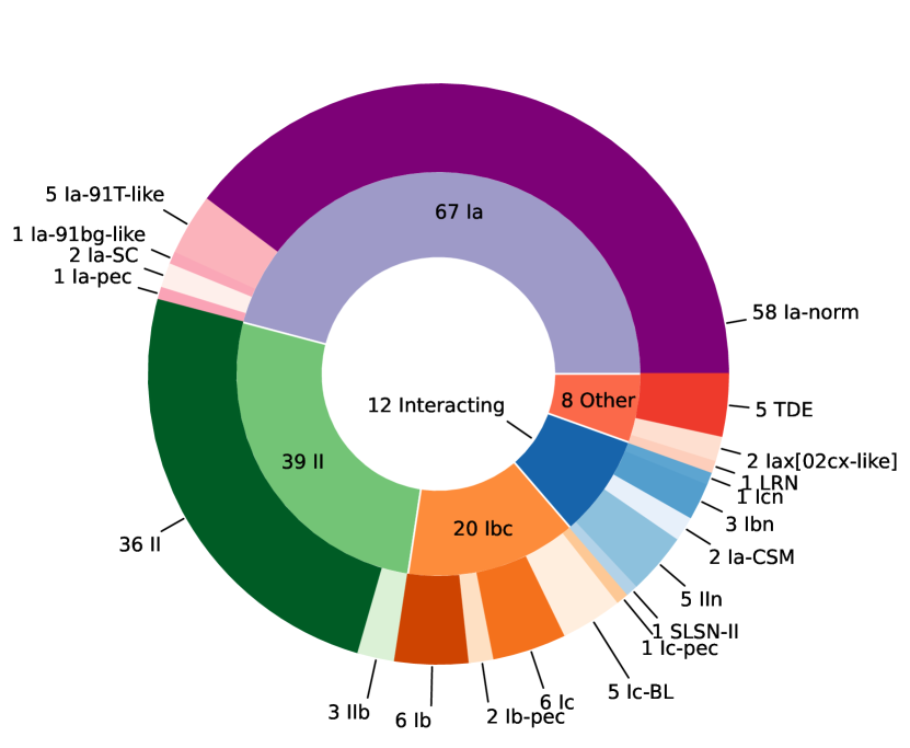
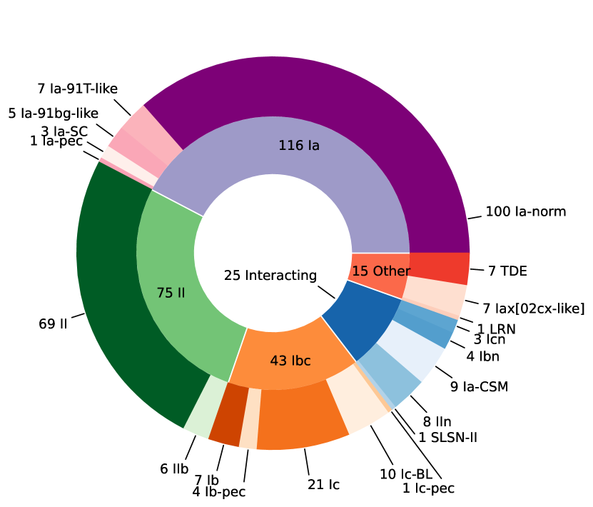
Full KITS Sample
By Unique Objects By Spectra This Data Release
    

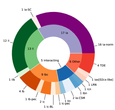
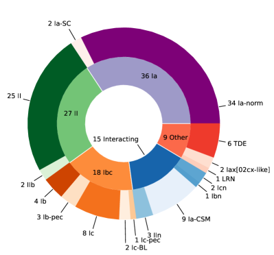
Figure 1: Pie charts showing numbers of SN types observed with KITS by unique events (left) and individual spectra (light). The top row includes the entire KITS sample (274 spectra from 146 objects) while the bottom row includes objects and spectra from this data release (105 spectra from 50 objects).

2 Survey Strategy

The overarching goal of KITS is to provide a large, publicly accessible NIR spectroscopic treasury of all types of astrophysical transients. This program is in direct support of the mission success criteria of both Roman and JWST.

A key science driver of Roman is to measure the expansion history of the Universe through luminosity-distance measurements. Roman’s High-Latitude Time Domain Survey is designed to discover and measure distances to thousands of SNe Ia (Hounsell et al., 2018; Rose et al., 2021). For $z<1$, Roman will observe the rest-frame NIR. Our distance-measurement techniques require a training set containing precise SED surfaces that span the wavelength, phase, and light-curve parameters of the the full SN Ia parameter space. The lack of SN Ia NIR spectra previously prevented accurate spectral models at these wavelengths (Pierel et al., 2022). KITS addresses this issue by providing the necessary spectra to be incorporated into the models through the SALTShaker training process outlined in Kenworthy et al. (2021). This will allow us to better plan for Roman and better leverage its data.

Major goals for JWST are to detect the most distant and luminous objects in the Universe, determine when the first stars were born, and constrain the timing of the epoch of reionization (Gardner et al., 2006). SNe, and in particular exotic, luminous SNe, may be the most-distant objects that will be discovered. Since these objects can occur only a few Myr after the first stars are formed, they can shine brighter than their nascent host galaxies and potentially be discovered at higher redshifts than galaxies. These explosions will also provide large amounts of ionizing photons, and measuring the rates and energetics of these SNe will determine their contribution to reionization. Even at $z\approx 20$, MIRI observes the rest-frame NIR, and accurate optical/NIR SEDs are necessary to identify and characterize high-redshift SNe that are too faint for spectroscopy.

Additionally, GO programs for both missions will undoubtedly study all other classes of transients, and NIR spectra will be critical to their understanding. We planned KITS to obtain NIR spectra of rare events and of common events in epochs at which NIR spectra are rare. These data will serve as comparison templates for new NIR observations of any transients from the ground or space. They will also help with photometric classification of high-redshift transients that Roman or JWST may serendipitously detect in the future.

In order to accomplish these goals, KITS focuses on three samples: (a) a flux-limited sample containing all transients brighter than 17 mag in a red optical band (usually ZTF $r$ or ATLAS $o$); (b) a volume-limited sample of all transients with $z<0.01$; (c) and SNe Ia with light-curve parameters or phases that are poorly sampled in the NIR. Lastly, we aim to observe rare transients with little to no prior NIR spectroscopy. We have used our target-of-opportunity (ToO) observations to further obtain NIR spectra of very young transients. Throughout the survey, we kept track of our progress for each subsurvey and adjusted our strategy to maximize the completeness and potential scientific output of our data, using YSE PZ, our in-house open-source target and observation management system (Coulter et al., 2022, 2023). We select transients discovered by the aforementioned public transient surveys.

3 Observations

KITS operated over about 12 half nights per semester in the 2022A (2022 Feb–Jul), 2022B (2022 Aug–2023 Jan), and 2023A (2023 Feb–Jul) semesters, with observations occurring roughly once every two weeks. All observations in 2022A and 2022B were in the second half of the night, while 2023A observations were in the first half. The last night of 2023A (2023 July 29 UT) was the only full-night observation. We obtained four ToO spectra with KITS to observe objects at crucial phases (e.g., young objects, or SNe Ia at previously unobserved phases). Table 1 summarizes all KITS nights and Table 2 lists all SNe observed by KITS in the 2022A semester.

All spectra (except one) were obtained with the Near-InfraRed Echellette Spectrometer (NIRES) on the Keck II telescope. NIRES is the latest member of the TripleSpec family of four NIR spectrographs. Wilson et al. (2004) provides an overview of this design. To make the same spectrograph optics work on different telescopes with different focal ratios, fore optics are installed to convert the incoming beam from the telescope to a uniform $f$/10.7. With Keck’s large aperture, the field of view decreases proportionally. NIRES’s single slit is $0.55^{\prime\prime}\times 18^{\prime\prime}$, and the slit-viewing camera has a field of view (FoV) of only $1.8^{\prime}\times 1.8^{\prime}.$ As a result of the small slit-viewing camera FoV, NIRES has an off-axis optical guide camera to help ensure that there is a star on which to guide. Crucially, the position angle (PA) of NIRES has to be selected such that there is a bright guide star in the FoV of the guide camera.

We follow a standard procedure for the observations to ensure the uniformity of data quality, which we outline below. For each night of observation, collaboration members query the database on YSE PZ for all transients that fall into our aforementioned subsamples, and request observations. The observer in charge downloads all observation requests from YSE PZ and runs a number of Python scripts to create finder charts with offset stars, to select a PA with a guide star in the guider, and to search for a nearby A0 V star necessary to correct for telluric absorption. The script also computes the rising/setting time of each target (taking into account Keck II’s western pointing limit owing to the Nasmyth platform), suggested exposure times, Moon distance, and the telescope azimuth wrap in which the target is observable. We schedule the night using these outputs, which help us maximize the observing efficiency. These scripts and their documentation are publicly available for other NIRES users.

Table 1: KITS Observation Log

UT Date	Night Half	Hours available	Targets
2022-02-13	second	5.5	9
2022-02-22	second	5.4	9
2022-03-11	second	5.2	8
2022-03-24	second	5.1	10
2022-04-15	second	4.9	9
2022-04-22	second	4.8	0
2022-05-09	second	4.7	8
2022-05-17	MOSFIRE ToO	1.0	1
2022-05-20	second	4.6	0
2022-06-07	second	4.5	10
2022-06-11	ToO	1.0	2
2022-06-22	second	4.4	7
2022-07-09	second	4.5	8
2022-07-19	second	4.5	11
2022-08-05	second	4.7	9
2022-08-18	second	4.8	9
2022-09-09	second	5.0	8
2022-09-18	second	5.1	8
2022-10-06	second	5.3	10
2022-10-15	second	5.4	7
2022-11-06	second	5.5	8
2022-11-17	second	5.6	12
2022-11-18	ToO	1.0	2
2022-12-01	second	5.6	3
2022-12-15	second	5.7	6
2022-12-31	second	5.7	14
2023-02-01	first	5.5	0
2023-02-08	first	5.5	8
2023-02-27	first	5.3	0
2023-03-12	first	5.2	0
2023-03-30	first	5.1	9
2023-04-07	ToO	1.0	1
2023-04-10	first	4.9	10
2023-04-27	first	4.8	5
2023-05-05	first	4.7	11
2023-05-28	first	4.5	11
2023-06-07	first	4.5	7
2023-07-05	first	4.5	7
2023-07-29	full	9.2	17

For each observing night, we obtain flat-field images using the dome-flat lamp. We find that using ten standard flat exposures, 120 s each, is sufficient. Flats with the lamp off (“dark frames”) are unnecessary because at this exposure time, the lamp-off flats have significant flux in the $K$ band, and do not capture the dark current. Observations of comparison lamps are also not necessary (but always taken) because we use IR night-sky lines to perform wavelength calibrations.

At the beginning of the night, the operator runs the MIRA software to focus the telescope. To acquire each target, we first take a pair of images of the target field with the slit-viewing camera. We are developing a pipeline that can automatically reduce NIRES slit-viewing camera images and use them to measure photometry. This will be included in the next data release. We identify the target and offset the telescope to place the target in the slit. Another image is taken for confirmation, and then the spectroscopic sequence is started, using exposure times suggested by our observation preparation script. All science observations are performed in an ABBA dithering pattern with the A and B positions $6^{\prime\prime}$ apart on the slit. This observing strategy allows us to subtract the bright NIR sky lines. For some observations, we perform two cycles of ABBA or simply an additional AB pair, with the determining factors being the total exposure time and the restriction that individual exposures be at most 300 s due to the saturating sky lines. Immediately before or after each science observation, we also obtain a spectrum of an A0 V star for flux and telluric calibration. These stars are also observed with an ABBA pattern, but with a $10^{\prime\prime}$ offset to prevent persistence from observing a bright star to interfere with subsequent science observations.

One ToO spectrum of SN 2022jzc on 2022 May 17 was obtained using the Multi-Object Spectrometer for Infra-Red Exploration (MOSFIRE; McLean et al., 2012) in the long-slit configuration with a $0.7^{\prime\prime}$ slit width. With MOSFIRE, spectra are obtained one filter at a time, and within the 1 hr interrupt we only had sufficient time to observed in the $Y$, $J$, and $K$ bands. A similar calibration procedure was followed for the MOSFIRE observation.

In parallel to Keck/NIRES observations, we also obtain observations of very bright objects using the SpeX spectrograph (Rayner et al., 2003) on the 3 m NASA InfraRed Telescope Facility (IRTF), and the TripleSpec spectrograph on the 4.1 m Southern Astrophysical Research (SOAR) Telescope. These observations are not included in the discussion of KITS in this paper, but will appear in the next and final data release.

Table 2: KITS 2022A Transients

AT/SN	RA    (J2000)	Dec    (J2000)	Spec. Type	Redshift	Ref MJD	Ref MJD Type	$N_{\rm obs}$	Reference
2020ohl	17:03:36.5	+62:01:32.34	TDE	0.01671	59014.4	explosion	1	Hinkle et al. (2020, 2022)
2021biy	12:42:04.0	+32:32:07.87	LRN	0.002021	59244.5	explosion	1	Cai et al. (2022)
2022fw	12:23:54.0	-03:26:37.88	SN Ia	0.0067	59601.9	peak	4	Hosseinzadeh et al. (2022)
2022jo	13:00:37.7	+28:03:25.76	SN II	0.0265	59581.5	explosion	1	Li et al. (2022a)
2022mm	11:58:25.1	-14:31:11.50	SN II	0.013	59590.0	explosion	1	Reguitti et al. (2022)
2022abq	13:22:56.8	+28:19:08.87	SN II	0.007979	59599.5	explosion	2	Ochner et al. (2022)
2022afc	07:56:45.0	+26:53:07.36	SN Ib	0.028	59621.0	peak	1	Davis et al. (2022b)
2022ann	10:17:29.7	-02:25:35.44	SN Icn	0.049	59609.6	peak	2	Davis et al. (2023)
2022baw	12:48:50.2	+37:14:51.76	SN Ia	0.04	59622.6	peak	1	Tucker (2022a)
2022bck	13:24:35.1	-20:11:07.48	SN Ib	0.026	59627.8	peak	1	Lyman et al. (2022)
2022bdu	09:36:52.2	+37:41:38.99	SN Ic	0.015	59628.0	peak	2	Tucker (2022a)
2022bdw	08:25:10.4	+18:34:57.50	TDE	0.03782	59632.0	peak	1	Arcavi et al. (2022a)
2022bse	07:01:02.3	+51:15:55.68	SN II	0.020954	59618.5	explosion	1	Srivastav et al. (2022)
2022crr	15:24:49.1	-21:23:21.73	SN Ic-BL	0.0188	59636.1	peak	2	Davis et al. (2022a)
2022crv	09:54:25.9	-25:42:11.16	SN Ib	0.008091	59647.0	peak	1	Andrews et al. (2022)
2022cvr	14:01:21.6	+37:18:56.97	SN Ia	0.064	59640.9	peak	1	SNIascore (2022a)
2022dbl	12:20:45.0	+49:33:04.68	TDE	0.0284	59639.3	peak	2	Arcavi et al. (2022b)
2022dml	16:17:29.1	+14:25:04.61	SN II	0.03	59635.0	explosion	1	Taggart (2022a); Burke et al. (2022)
2022dsb	15:42:21.7	-22:40:14.04	TDE	0.023	59630.0	explosion	2	Fulton et al. (2022c)
2022dtv	14:36:35.2	+11:56:21.40	SN Ia	0.028617	59654.0	peak	2	Hinds & Perley (2022)
2022eat	11:11:31.0	+19:49:38.17	SN Ia	0.027	59657.8	peak	2	Chu et al. (2022)
2022erq	18:33:25.4	+44:05:11.65	SN Ia-CSM	0.066	59682.0	peak	6	Li et al. (2022b)
2022erw	10:50:57.8	-02:08:59.28	SN Ia	0.015	59664.0	peak	1	Moore et al. (2022)
2022esa	16:53:57.6	-09:42:10.26	SN Ia-CSM	0.023	59709.5	peak	3	Lu et al. (2022)
2022ewj	10:46:34.6	+13:45:17.03	SN II	0.010134	59655.0	explosion	1	Tagchi (2022)
2022exc	17:15:02.1	+60:12:58.79	SN Ia	0.020123	59671.1	peak	5	Do (2022)
2022eyj	11:18:00.6	+07:50:44.66	SN Ia	0.021103	59662.5	peak	1	Balcon (2022a)
2022eyw	12:43:60.0	+62:19:48.29	SN Iax	0.009	59678.8	peak	2	Tagchi et al. (2022)
2022fcc	14:15:54.8	+03:36:14.60	SN Ia	0.025851	59682.0	peak	1	Pellegrino et al. (2022a)
2022frl	15:21:33.1	-07:26:52.04	SN Ib-pec	0.006	59691.8	peak	3	Tucker (2022b)
2022frn	12:59:51.8	+27:56:36.66	SN Ia	0.023	59684.1	peak	2	Balcon (2022b); Fulton et al. (2022a)
2022hrs	12:43:34.3	+11:34:35.87	SN Ia	0.0047	59698.5	peak	3	Balcon (2022c)
2022hsu	22:11:37.7	+46:18:40.03	SN IIn	0.018	59710.8	peak	3	Ashall (2022a); Taggart (2022b)
2022ihx	19:16:38.4	+61:41:15.48	SN Ibn	0.033	59700.1	peak	1	Pellegrino et al. (2022b)
2022iid	18:15:38.7	+73:08:06.05	SN II	0.014	59701.5	explosion	3	Fulton et al. (2022b)
2022ilv	15:10:44.3	-11:35:57.99	SN Ia-SC	0.031	59707.2	peak	2	Srivastav et al. (2023)
2022jli	00:34:45.7	-08:23:12.16	SN Ic	0.006	59704.2	discovery	6	Monard (2022); Grzegorzek (2022)
2022joj	14:41:40.1	+03:00:24.33	SN Ia	0.03	59724.1	peak	1	Newsome et al. (2022)
2022jzc	12:05:28.67	+50:31:36.80	SN II	0.0029	59714.3	explosion	1	Bruch et al. (2022)
2022kla	16:44:33.2	+38:55:03.25	SN Ia	0.037112	59734.8	peak	2	SNIascore (2022b)
2022lxg	19:15:23.6	+48:19:27.70	SN II	0.0214	59731.5	explosion	4	Ashall (2022b), this work
2022mji	09:42:54.1	+31:51:03.67	SN II	0.004	59731.9	explosion	1	Sollerman et al. (2022a)
2022mxv	23:51:05.1	+20:09:08.96	SN II	0.014046	59745.5	explosion	6	Davis et al. (2022c)
2022mya	17:21:08.1	+16:03:32.47	SN Ib	0.03	59759.1	peak	1	Sollerman et al. (2022b)
2022nag	18:05:00.7	+09:28:47.86	SN Ia	0.020954	59757.1	peak	3	SNIascore (2022c)
2022ngb	18:56:51.5	+36:37:07.82	SN IIb	0.009	59777.6	peak	2	Izzo et al. (2022)
2022ojo	01:44:35.6	+37:41:50.72	SN II	0.019	59755.5	explosion	3	Desai (2022)
2022oqm	15:09:08.2	+52:32:05.14	SN Ic-pec	0.012	59783.9	peak	1	Irani et al. (2022)
2022osg	20:29:49.0	-02:01:41.11	SN Ia	0.01858	59785.1	peak	2	Lidman et al. (2022)
2022ovq	02:01:59.9	+21:06:23.45	SN Ia	0.030298	59786.4	peak	3	Hinkle (2022)

4 Data Reduction

The data are typically downloaded the following day and we process them for quick quality assessment using IDL software spextool (Cushing et al., 2004) and xtellcor (Vacca et al., 2003), which are standard in NIR spectroscopy. While widely used and well tested, spextool and xtellcor require intensive user input to extract data and perform telluric correction. They also require a paid IDL license to run. In order to perform a uniform data reduction for this public data release, and make our process as reproducible as possible, we uniformly reprocess our data using the much more autonomous Python-based open-source facility spectroscopic reduction software Pypeit (Prochaska et al., 2020a, b). We specifically use v.1.13.0, which has many useful functionalities to support NIRES observations.

There are three steps to process a night of data with Pypeit: preparation, spectral extraction, and calibrations. We follow the Pypeit documentation, and wrote additional helper scripts to make the process more automated. In the preparation step, Pypeit goes through the raw data directory and classifies files as science, standard, or different types of calibration. Pypeit can also figure out the dither pattern used in the observations and automatically assign a background frame for subtraction. The script outputs a setup file summarizing the observing log for a user to verify that everything is correct. We remove dome flats with lamp off and wavelength comparison-lamp frames from this file, so they do not get processed further. We also add two flags to ask Pypeit to only attempt to find one source in each science and standard frame in the next step.

After the preparation is done and we have verified that everything in the setup file is correct, we can execute this file by running the run_pypeit command. This takes about 2 hr on our computer node, but could take up to several hours on a personal computer. The script creates a master flat field using dome-flat observations. Dome flats are also used to identify the illuminated area of the detector. The script uses night-sky emission lines in science frames to perform wavelength calibration and measure the tilt of the spectra. Standard observations automatically get assigned wavelength solution from the science observations closest in time and airmass. It is crucial to note that Pypeit provides wavelengths in vacuum, and not in air as is typical for NIR lines. After all the calibrations are prepared, Pypeit goes through all science and standard exposures, applies these calibrations, automatically identifies a source, and performs spectral extraction. The resulting extracted spectra are stored in spec1d files, along with calibrated two-dimensional (2D) spectra in spec2d files.

The last step is to calibrate the extracted spectra to go from extracted 1D spectra to flux-calibrated, telluric-corrected, science-ready spectra. Pypeit provides commands to do each step separately, and some steps also need a separate parameter file. To speed up the process, we wrote a Python script to create a bash script containing all commands we need to perform all these calibrations to all our data, along with necessary parameter files. It also matches science targets to an appropriate telluric star.

Pypeit first computes the sensitivity function by comparing observations of each A0 V star to a model spectrum and the telluric absorption spectrum at Maunakea. This sensitivity function is then used to flux calibrate and coadd science observations. The coaddition step also stitches different orders of the spectrum together. We then fit the telluric model to the A0 V star observation using a telluric model grid specifically for Maunakea supplied by Pypeit. In this step, we found that we need to add an optional parameter polyorder = 5 to the default telluric parameter file to get a good fit. This is the order of a polynomial used to approximate the star’s continuum across hydrogen absorption lines.

Finally, the telluric model is applied to the science observation to produce a final, science-ready spectrum. This last step is not currently supported by Pypeit. It can fit a telluric model to the science spectrum and apply the resulting model to the same spectrum. For a generic target, this method normally uses a polynomial to approximate the science spectrum. This method does not work for SN spectra, which often have spectral features coinciding with the telluric absorption lines, especially the $\rm CO_{2}$ lines around 2 $\mu$m coinciding with the He 2.0581 $\mu$m line. We have another custom python script to take the telluric model fitted to a standard-star observation and apply it to a corresponding science observation. However, this is the step in which further pipeline development can improve the resulting spectra quality.

To get from raw data to the final calibrated NIRES spectrum for each night, the user only needs to run three different commands and manually check two intermediate setup files. This workflow considerably reduces the workload and active time required to process a night of observation in comparison to running spextool (which usually takes an entire day to reduce data from one half night), and ensures that the resulting spectra are reproducible.

5 Observed Sample

5.1 Observed Classes

Figure 1 displays pie charts conveying the fractions of the KITS sample that correspond to different transient classes. We present these fractions for distinct objects and observed spectra, both for the full KITS sample and what is included in the first data release (corresponding to semester 2022A). In total, we obtained 274 spectra of 146 objects. This data release contains 105 spectra of 50 objects. In addition to the common SN classes, we observed a number of rare transients, including 2 SNe Iax, 2 “super-Chandrasekhar” SNe Ia, 4 TDEs, 1 luminous red nova (LRN), 3 SNe Ibn, and 1 SN Icn. Data for all four TDEs (AT 2020ohl, 2022bdw, 2022dbl, and 2022dsb), the LRN (AT 2021biy), one SN Iax (SN 2022eyw), and one SN Ibn (SN 2022ihx) are included in this data release. Data for three objects — SNe 2022ann (Type Icn), 2022oqm (a peculiar, calcium-rich SN Ic), and 2022joj (peculiar SN Ia) — have already been published by Davis et al. (2023), Yadavalli et al. (2023), and Padilla Gonzalez et al. (2023), respectively, and for completeness we include those data as part of this data release. In addition, KITS observations from later semesters of SN 2022pul have been used in conjunction with JWST observations to study its peculiar nature (Siebert et al., 2023; Kwok et al., 2023).

The release of the full sample is expected in mid-2024. The full release will include spectra from IRTF/SpeX and SOAR/TripleSpec, further improving the NIR spectroscopic coverage of our sample. It will also include photometry of KITS objects from the slit-viewing camera of NIRES, and Gemini NIRI and FLAMINGOS-2.

5.2 Completeness of the flux- and volume-limited samples

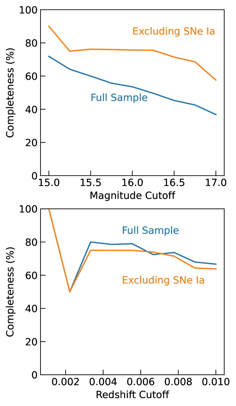
Figure 2: KITS completeness as a function of maximum magnitude in any reported visible bands, most commonly $r$ or ATLAS $o$ P(top) and maximum redshift (Bottom). The completeness of the full sample is plotted in blue and that excluding SNe Ia is plotted in orange.

As described in Section 2, a main goal of KITS is to survey the full variety of transients without regard to class. Flux- and volume-limited samples are ideal ways to produce samples of rare objects with easily understood selection effects. A volume-limited sample targets low-luminosity transients that could be missed in a flux-limited survey. A flux-limited survey can access rare (and luminous) objects that may not occur in a relatively small volume.

We determine the full volume-limited sample by querying YSE PZ for all transients with $z<0.01$ that are discovered between $<2$ weeks before our first night and on our last night. For the flux-limited sample, we run a similar query but require a peak magnitude from any public survey of $<17$ mag in the visible (typically either the ZTF $r$ band or ATLAS $o$ band). While this selection should ideally have been done in the NIR, the present lack of such NIR facility for time-domain astronomy prevented us from doing so. We went through every object on YSE PZ to ensure that the photometric point used to determine the peak magnitude is not spurious. Objects with TNS classifications CV, VarStar, Nova, and “Other” are excluded. We also exclude objects with $\delta<-30^{\circ}$, which are not easily visible from Keck. Moreover, we exclude objects that are not visible during the half-nights allocated to KITS. There are only 7 objects in the flux-limited sample and 1 objects in the volume-limited sample that fall into this category, so excluding them does not affect the completeness significantly. The fraction of these objects that has at least one NIRES spectrum is our completeness.

Figure 2 shows the completeness of our flux- and volume-limited samples. The top panel shows the completeness as a function of a magnitude cutoff and the bottom panel indicates the completeness as a function of a redshift cutoff. Our volume ($z<0.01$) and flux ($r$/$o$ $<17$ mag) limited samples are 37% (103/280 objects observed) and 54% (41/76 objects observed) complete, respectively. The flux-limited sample is dominated by SNe Ia. Because of their homogeneity and the limited observing time, we did not observe the majority of SNe Ia in the flux-limited sample near peak brightness. The flux-limited sample, excluding SNe Ia, is 58% complete (53/92 objects observed). The completeness fraction of the flux-limited sample, excluding SNe Ia, improves to 71% at 16.5 mag, while the volume-limited sample (including SNe Ia) is 79% complete at $z=0.005$. Furthermore, bright objects missing from the flux-limited sample have been observed with IRTF/SpeX or SOAR/TripleSpec. Data from those observations, along with the improved statistics, will be available with the next data release.

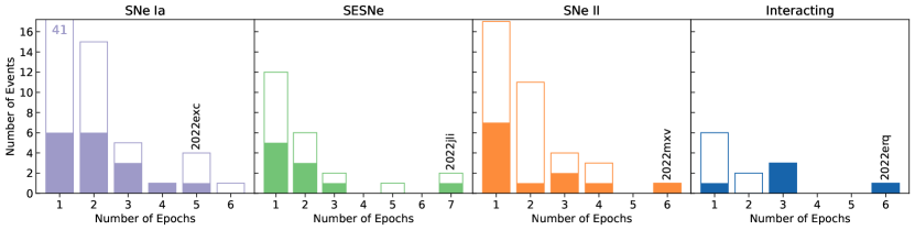
Figure 3: Histograms showing the distribution of number of KITS spectra per SN for different SN subtypes. The full sample is shown in unfilled bars; those included in this data release are filled. The object in this data release with the most observations in each type is labeled in the plot. The left panel for SNe Ia includes normal SNe Ia, 91T-like, 91bg-like, and super-Chandra, while excluding SNe Iax. The middle-left panel for SESNe includes SNe IIb, Ib, Ic, and Ic-BL, along with objects labeled peculiar. The middle-right panel includes all SNe II that are not IIb or IIn. Finally, the right panel includes SNe Ia-CSM, Ibn, Icn, and IIn. We attempt to obtain multiple spectra for every object, but in many cases it was not possible owing to (for example) the visibility constraint, the source fading, or scheduling issues.

Figure 4: Histograms showing the distribution of redshift of SNe observed by KITS, with SNe Ia, SESNe, SNe II, and interacting objects plotted from left to right (same subtypes as plotted in Fig. 3). The full sample is shown in unfilled bars; objects included in this data release are filled.

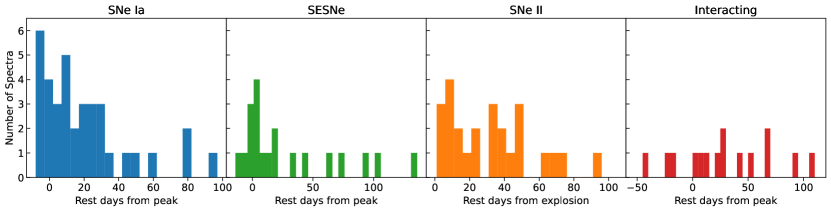
Figure 5: Histograms showing the distribution of phases of SN spectra observed by KITS, with SNe Ia, SESNe, SNe II, and interacting objects plotted from left to right. These only include spectra from this data release.

5.3 Sample Statistics

Figure 3 illustrates histograms of the number of observations per event for each common SN subtype. The full sample is shown, with the subset included in this data release indicated in shaded area. From left to right, we display histograms for SNe Ia, including all subtypes except the interacting SNe Ia-CSM; SESNe including Types IIb, Ib, Ic, and Ic-BL, along with peculiar hydrogen-poor events; SNe II, excluding the stripped SNe IIb; and interacting SNe, including Types IIn, Ibn, Icn, and Ia-CSM. The most well-observed objects of each type in this data release are labeled. They often are the most nearby or have peculiar evolution. Given the frequency of KITS nights and the fact that most of our time allocations are in half nights, we have a maximum of 7 spectra per object, and about 41% of all objects have only a single spectrum (primarily driven by SNe Ia). On average, we obtain 1.9 spectra per object. We highlight the SN Ia 2022exc, SN Ic-pec 2022jli, SN II 2022mxv, and SN Ia-CSM 2022erq, which have 5, 7 (6 included in this release), 6, and 6 spectra, respectively. These objects are particularly nearby and bright, and show peculiar evolution that warrants multi-epoch observations.

Figure 4 displays redshift distributions for each broad class mentioned above. Similar to the last figure, the full sample is shown unfilled with DR1 objects in the shaded area. The median redshifts are 0.0298 for SNe Ia, 0.03 for SESNe, 0.0094 for SNe II, and 0.0355 for interacting SNe (full sample). The maximum redshifts are 0.064 for SNe Ia (SN 2022cvr), 0.064 for SESNe (SN 2023mee), 0.03 for SNe II (SN 2022dml), and 0.08 for interacting SNe (SN 2023gpw). Because of the overabundance of SNe Ia in the flux-limited sample, we focused on those objects that could either potentially have their luminosity calibrated through direct distance measurements (i.e., Cepheid or tip-of-the-red-giant-branch measurements, corresponding to $D\lesssim 40$ Mpc) or those clearly in the Hubble flow ($z>0.015$). Nevertheless, our choices for the flux- and volume-limited sample result in almost all normal SNe Ia having $z<0.04$, which would correspond to the “Physics” subsample of CSP II (Hsiao et al., 2019).

We use public photometry of each transient to determine the phase of the NIR spectra. We primarily use $o$-band ATLAS photometry as the vast majority of our targets are well observed. For the SNe II, TDEs, and LRNe that lack a clear time of maximum brightness, we define the phase relative to the “time of explosion,” which we define as the midpoint between the first detection and the last nondetection. For all other transients, we fit a low-order polynomial to the light curve to determine the peak epoch, from which we define their phase. However, there are a few exceptions to these general prescriptions. SN 2022jli was discovered soon after it rose for the observing season, indicating that it likely exploded when it was behind the Sun; thus, the phase is relative to the discovery epoch (Monard, 2022). SNe 2022hsu, 2022ihx, and 2022kla have poor ATLAS observations, and we use the ZTF $r$ light curve instead to define phase. SN 2022mji set soon after discovery, and thus has a poorly sampled light curve near discovery; we use the last nondetection from ATLAS and the first detection from Gaia to determine the explosion epoch. Table 2 provides the reference epoch and method for each transient; spectral phases are relative to this reference epoch.

Figure 5 shows distributions of phases of KITS spectra for each common SN subtype. We only display data from the DR1, corresponding to the transients for which we have measured a reference epoch. The median phases of our observation in DR1 are 12 days post-peak for SNe Ia, 11 days post-peak for SESNe, 33 days post-explosion for SNe II, and 26 days post-peak for interacting SNe. The minimum phases are 8 days before peak for SNe Ia (SN 2022exc); 14 days before peak for SESNe (SN 2022crv); 1 day post explosion for SNe II (SN 2022jzc, ToO observation); and 45 days before peak for interacting SNe (SN 2022esa). The maximum phases are 95 days post peak for SNe Ia (SN 2022exc), 135 days post-peak for SESNe (SN 2022jli), 93 days post-explosion for SNe II (SN 2022mxv), and 107 days post-peak for interacting SNe (SN 2022erq).

5.4 Observations of SNe Ia

The small extant sample of SNe Ia from before the start of KITS with high-quality, publicly available NIR spectra is only $\sim 50$ SNe, and with only $\sim 9$ SNe with well-sampled optical photometry appropriate for building a spectral model. Most of these spectra are from an unsystematic ensemble of SNe discovered through last-generation targeted SN searches and obtained in 2002–2005 with the 3-meter IRTF (Marion et al., 2009). The CSP II (Hsiao et al., 2019; Lu et al., 2023) obtained 331 NIR spectra of 94 normal SNe Ia with light curves and minimal host-galaxy contamination (Lu et al., 2023), dramatically increasing the available spectra for training; however, while the spectra have been publicly released, the corresponding light curves have not, preventing the inclusion of CSP II data in model training samples at this time.

Despite the promise of the NIR, the lack of a robust NIR spectral model means that current cosmological SN constraints exclusively use optical data (Scolnic et al., 2018; Riess et al., 2019; Abbott et al., 2019). Pierel et al. (2018) estimate that a sample of $\gtrsim 250$ SN Ia NIR spectra is necessary to include NIR data in dark-energy analyses. In addition to a large number of spectra, the SNe must also span the full parameter space of SN properties, requiring coverage in the combination of light-curve shape (e.g., $x_{1}$ for SALT3), color (e.g., $c$ for SALT3), and phase. Figure 6 displays the KITS coverage in these three parameters compared to the training sample of Pierel et al. (2022), considering only spectra with coverage beyond $\sim 1.2$ $\mu$m.

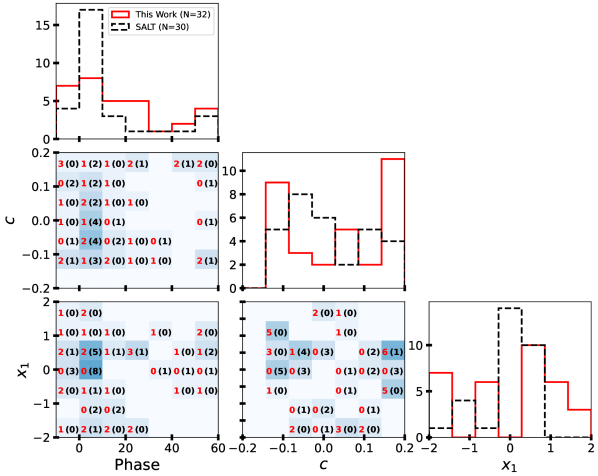
Figure 6: Relationships between SALT3 model parameters for the sample of SN Ia spectra with coverage beyond $\sim 1.2~{}\mu$m used in the training of Pierel et al. (2022) (black) and those presented in this work (red). 2D histograms show the combined sample in blue, with the individual contributions given as colored numbers.

6 The data

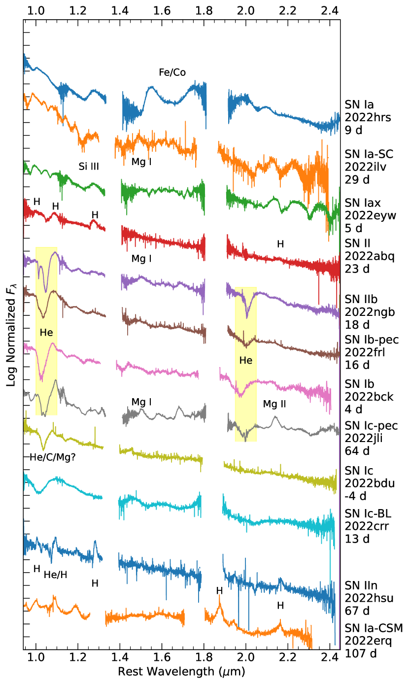
Figure 7: KITS spectra of different subtypes of SNe available in DR1. From top to bottom, we show different subtypes of thermonuclear explosions: normal SN Ia 2022hrs, a super-Chandra SN 2022ilv, and a Type Iax SN 2022eyq. Then we show different subtypes of CCSNe sorted by the level of stripping: from a Type II SN 2022abq; a partially-stripped Type IIb SN 2022ngb; a peculiar SN Ib 2022frl with some sign of hydrogen; a hydrogen-free Type Ib SN 2022bck; a peculiar Type Ic SN 2022jli with some signature of helium; a helium-poor Type Ic SN 2022bdu; and an energetic Type Ic-BL 2022crr. Finally, we show two interacting SNe: SN IIn 2022hsu and SN Ia-CSM 2022erq. Prominent hydrogen and helium lines are annotated in the plot. Most features in SN Ia spectra are due to iron and cobalt.

Spectra in DR1 are posted to WISEReP for easy access to the time-domain astronomy community. More data-reduction products are available via Zenodo (Tinyanont et al., 2023) to ensure that the final reduction is reproducible. Extracted and coadded one-dimensional spectra of both the transients and telluric standard stars from Pypeit are provided in FITS format. This allows users to repeat the flux and telluric calibration if necessary.

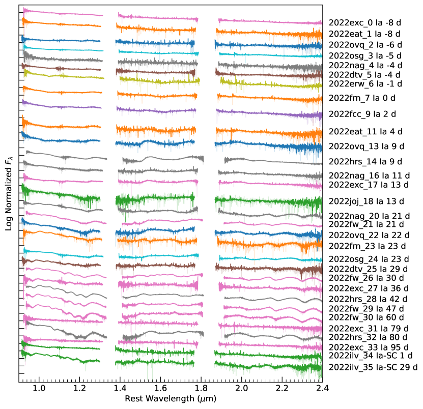
Figure 8: KITS spectra of SNe Ia included in DR1 sorted by phase of observation. SN name, subtype, and phase are labeled. The spectra are shown in $F_{\lambda}$ units, normalized and on a log scale. The super-Chandrasekhar event SN 2022ilv is plotted in the bottom. Spectra having poor signal-to-noise ratios are excluded. Some spectra have been smoothed, with the unsmoothed version shown in the background. We note that late-time spectra of SN 2022exc may have significant host-galaxy contamination as the SN is in a nuclear region.

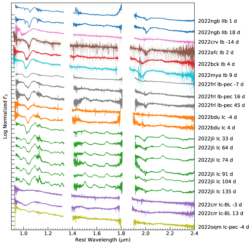
Figure 9: Same as Figure 8 but for SESNe. We order subtypes according to an increasing degree of stripping: hydrogen-poor type IIb, hydrogen-free Ib, and hydrogen-free and helium-poor Ic. The Ic-BL and peculiar Ic are plotted in the bottom.

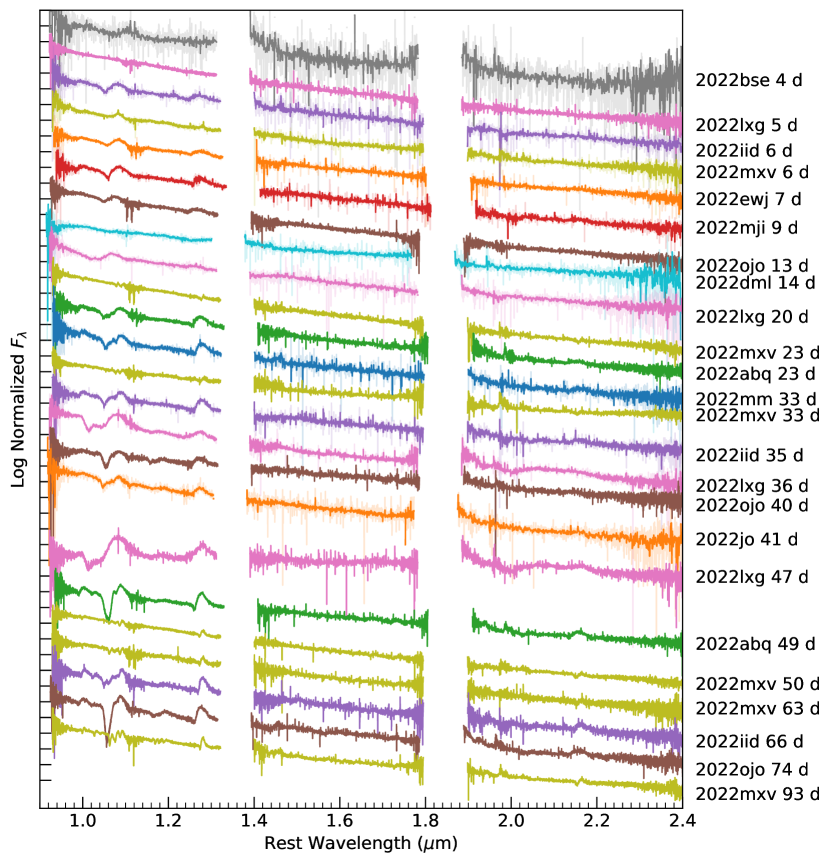
Figure 10: Same as Figure 8 but for SNe II.

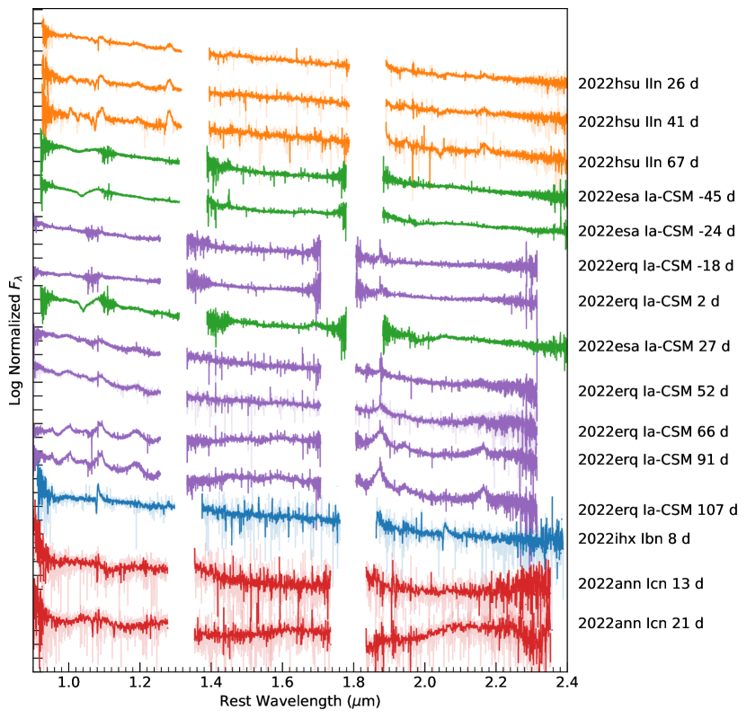
Figure 11: Same as Figure 8 but for interacting SNe.

To showcase our dataset, we plot representative spectra of different subclasses of SNe available in this data release in Figure 7, with important spectral lines labeled. We also plot most of the observed spectra from DR1 of SNe Ia, SESNe, SNe II, and interacting SNe in Figures 8, 9, 10, and 11, respectively. In addition to SNe, we plot spectra of TDEs and the LRN AT 2021biy in Figure 12. For TDEs, broad hydrogen features seen in the Balmer lines are not visible in the Paschen or Brackett lines for the spectra taken at similar epochs as the optical broad-line detections.

For SNe Ia, DR1 data only cover normal SNe Ia and one super-Chandrasekhar event (SN 2022ilv; Srivastav et al., 2023). The full KITS data set will cover other subtypes of SNe Ia. Spectra shown in Figure 8 show homogeneity, as expected from this class. The majority of spectral features seen in the NIR are from iron and cobalt. KITS’s contribution to SNe Ia is in the coverage of the light curve parameter space discussed in the previous section.

For SESNe, this dataset can probe the diminishing NIR helium features from Type IIb to Ib to Ic. The 2.0581 $\mu$m line is uncontaminated and unsaturated; thus, it could be used to measure the helium mass in the envelope at the time of core collapse (Dessart et al., 2020). Our dataset contains three peculiar objects. First, SN 2022frl is classified as a Type Ib SN; however, its NIR spectra contain clear hydrogen emission at all phases, resembling those of Type IIb SN 2022ngb (Figure 9). This indicated that SN 2022frl may have an ambiguous classification between Types IIb and Ib. SN 2022jli is classified as Type Ic in the optical, but NIR spectra show clear absorption associated with the He I 2.0581 $\mu$m line. The absorption trough of the He I 1.083 $\mu$m line also has a multicomponent structure with several distinct absorption troughs, which may indicate inhomogeneous ejecta. The last peculiar object is SN 2022oqm, which is more similar to calcium-rich transients than SNe (Yadavalli et al., 2023).

For SNe II, most data obtained with KITS (and all that are included in DR1) are during the plateau phase. The highlight of this dataset is the diverse absorption profile of the He I 1.0830 $\mu$m and hydrogen Pa$\gamma$ (1.0938 $\mu$m) complex. Some objects, such as SNe 2022lxg and 2022iid, show strong multicomponent absorption with a high-velocity component associated with CSM interaction (Chugai et al., 2007). We note that SN IIb 2022ngb also has a very strong high-velocity absorption, likely of both He I 1.0830 $\mu$m and Pa$\gamma$. Others, such as SNe 2022abq and 2022ojo, have a more typical P Cygni profile. We also noticed a peculiar spectral evolution for SN 2022mxv (which was classified using a KITS spectrum; Davis et al., 2022c), a luminous SN II with clear narrow emission lines from CSM interaction at early times. This is the only object for which the velocity remains low throughout its evolution such that the He I 1.0830 $\mu$m and Pa$\gamma$ are clearly separated for all phases. This indicates that the photosphere remains above the higher-velocity ejecta, and only the shocked CSM is observed. Another peculiar object is SN 2022lxg, which has a distinct profile for hydrogen lines, and flux excess in the $K$ band starting around 37 days post-explosion. This is normally far too early for an SN II to have dust form in the ejecta (e.g., Sarangi et al., 2018), but with the sign of CSM interaction detected at early times, we might be seeing CSM dust being heated. The fact that so many peculiar objects are identified in the limited set of objects included in DR1 highlights the relatively unexplored nature of NIR spectroscopy of transients.

For interacting SNe, the NIR allows for observations of isolated helium lines. As we discuss below, this leads to a discovery that the helium-poor interacting Type Icn SNe have a small amount of helium in the CSM. This data release also contains multi-epoch observations of two SNe Ia-CSM: SNe 2022erq and 2022esa. They are thought to be SNe Ia exploding in a dense hydrogen-rich medium. The NIR spectra of SN 2022erq, in particular, show complicated line profiles for the He I 1.0830 $\mu$m and Pa$\gamma$ complex, with very narrow absorption and emission components from both lines superimposed on broad electron-scattered lines.

KITS data have already led to five publications at the time of writing. Davis et al. (2023) presented KITS NIR spectroscopy of SN 2022ann, a member of the newly established class of hydrogen-free and helium-poor interacting SNe Icn, along with other optical observations. They found that the He I 1.083 $\mu$m line is unambiguously present in KITS NIR spectra at phases where the corresponding optical lines are not identifiable. Owing to the small velocities in the CSM, this helium line is not blended with the C I 1.0693 $\mu$m line, which is also detected. With these observations, they conclude that NIR spectra provide stronger constraints on the presence of helium in SNe Icn than optical-only datasets. Yadavalli et al. (2023) presented KITS NIR spectroscopy of SN 2022oqm, a peculiarly luminous calcium-rich transient (CaRTs). The nondetection of the He I 2.0581 $\mu$m line in the KITS NIR spectrum was used to argue that SN 2022oqm has a particularly helium-poor atmosphere, unlike other CaRTs, which normally have strong helium features. This allowed for important constraints on the progenitor system. The obtained KITS NIR spectrum is also one of the earliest NIR spectra of a CaRT, allowing for a better probe of the early-time NIR evolution. Padilla Gonzalez et al. (2023) used KITS data to explore the presence of unburned helium by detecting the He I 1.0830 $\mu$m line in SN 2022joj. Recent simulations have highlighted the potential occurrence of unburned helium in both single and double detonations within the outer ejecta. Consequently, given the indications that SN 2022joj exhibits characteristics consistent with a potential double detonation event, the investigation of this line becomes pivotal. Model comparison to the KITS spectrum constrained the helium shell mass to around 0.02 $M_{\odot}$. Siebert et al. (2023) presented KITS nebular spectroscopy of SN 2022pul (a “super-Chandrasekhar”-mass SN Ia) along with nearly simultaneous NIR and MIR spectroscopy from JWST. The higher resolution of the KITS data in the NIR was critical for constraining velocity distributions of IGEs in the SN ejecta. Kwok et al. (2023) found that IGE emission-line profiles tended to be redshifted while intermediate-mass element emission-line profiles were blueshifted. This supported their conclusion that SN 2022pul was the result of the violent merger of two white dwarfs. Additionally, given that the JWST data reveal a strong thermal dust continuum in SN 2022pul (Siebert et al., 2023), Johansson et al. (2023, in prep.) further analyzed the KITS data to constrain the presence of CO emission.

Figure 12: Similar to Figure 8 but for the LRN AT 2021biy and the TDEs in the sample. The right panel zooms in around the bandheads of the carbon monoxide first overtone to demonstrate the absorption detected in all objects. In the LRN, this could be local to the explosion, while for the TDEs this is likely due to other stars in the galactic nucleus.

7 Summary

The first KITS data release included in this work consists of 105 NIR spectra from 50 transients. We aim to provide KITS data in a timely manner, with the data released 1–2 yr after they were obtained. To meet this fast timeline, the data release is limited in scope. Future data releases will include additional NIRES spectra, NIRES NIR photometry, NIR spectra from IRTF/SpeX and SOAR/TripleSpec, Gemini/FLAMINGOS2 photometry, and photometry and spectroscopy from other sources.

The KITS survey design combined with unbiased discovery surveys resulted in a diverse set of astrophysical transients beyond previous NIR datasets that existed in the literature. The last large-scale NIR spectroscopic survey of SNe, CSP-II, concluded in 2015, and KITS provides NIR spectra of a contemporary sample of transients that include newly discovered classes of objects. This dataset will serve as a stepping stone to analyze JWST observations of high-redshift transients, and to plan the time-domain survey for Roman for next-generation cosmological studies using Type Ia SNe in the NIR. With the full data release expected in 2024, KITS data will account for a significant portion of NIR spectra of transients. This will contribute to the NIR spectroscopic treasury, against which new observations can be compared to reveal patterns and features previously invisible to us.

References

- Abbott et al. (2019) Abbott, T. M. C., Allam, S., Andersen, P., et al. 2019, ApJ, 872, L30, doi: 10.3847/2041-8213/ab04fa
- Andrews et al. (2022) Andrews, J. E., Lundquist, M., Sand, D. J., et al. 2022, Transient Name Server Classification Report, 2022-454, 1
- Arcavi et al. (2022a) Arcavi, I., Dgany, Y., & Pellegrino, C. 2022a, Transient Name Server AstroNote, 50, 1
- Arcavi et al. (2014) Arcavi, I., Gal-Yam, A., Sullivan, M., et al. 2014, ApJ, 793, 38, doi: 10.1088/0004-637X/793/1/38
- Arcavi et al. (2022b) Arcavi, I., Dgany, Y., Pellegrino, C., et al. 2022b, Transient Name Server Classification Report, 2022-504, 1
- Ashall (2022a) Ashall, C. 2022a, Transient Name Server Classification Report, 2022-1280, 1
- Ashall (2022b) —. 2022b, Transient Name Server Classification Report, 2022-1602, 1
- Balcon (2022a) Balcon, C. 2022a, Transient Name Server Classification Report, 2022-756, 1
- Balcon (2022b) —. 2022b, Transient Name Server Classification Report, 2022-903, 1
- Balcon (2022c) —. 2022c, Transient Name Server Classification Report, 2022-997, 1
- Bellm et al. (2019) Bellm, E. C., Kulkarni, S. R., Graham, M. J., et al. 2019, PASP, 131, 018002, doi: 10.1088/1538-3873/aaecbe
- Brout & Scolnic (2021) Brout, D., & Scolnic, D. 2021, ApJ, 909, 26, doi: 10.3847/1538-4357/abd69b
- Brout et al. (2019) Brout, D., Scolnic, D., Kessler, R., et al. 2019, ApJ, 874, 150, doi: 10.3847/1538-4357/ab08a0
- Bruch et al. (2022) Bruch, R., Sollerman, J., Zimmerman, E., et al. 2022, Transient Name Server AstroNote, 108, 1
- Burke et al. (2022) Burke, J., Li, W., Howell, D. A., et al. 2022, Transient Name Server Classification Report, 2022-567, 1
- Cai et al. (2022) Cai, Y. Z., Pastorello, A., Fraser, M., et al. 2022, A&A, 667, A4, doi: 10.1051/0004-6361/202244393
- Chu et al. (2022) Chu, M., Dahiwale, A., & Fremling, C. 2022, Transient Name Server Classification Report, 2022-659, 1
- Chugai et al. (2007) Chugai, N. N., Chevalier, R. A., & Utrobin, V. P. 2007, ApJ, 662, 1136, doi: 10.1086/518160
- Coulter et al. (2022) Coulter, D. A., Jones, D. O., McGill, P., et al. 2022, YSE-PZ: An Open-source Target and Observation Management System, v0.3.0, Zenodo, Zenodo, doi: 10.5281/zenodo.7278430
- Coulter et al. (2023) —. 2023, PASP, 135, 064501, doi: 10.1088/1538-3873/acd662
- Cushing et al. (2004) Cushing, M. C., Vacca, W. D., & Rayner, J. T. 2004, PASP, 116, 362, doi: 10.1086/382907
- Davis et al. (2022a) Davis, K., Foley, R., & Dimitriadis, G. 2022a, Transient Name Server Classification Report, 2022-520, 1
- Davis et al. (2022b) Davis, K., Johnson, J., Tinyanont, S., et al. 2022b, Transient Name Server Classification Report, 2022-362, 1
- Davis et al. (2022c) Davis, K. W., Tinyanont, S., Foley, R. J., & Chornock, R. 2022c, The Astronomer’s Telegram, 15464, 1
- Davis et al. (2023) Davis, K. W., Taggart, K., Tinyanont, S., et al. 2023, MNRAS, 523, 2530, doi: 10.1093/mnras/stad1433
- Davis et al. (2019) Davis, S., Hsiao, E. Y., Ashall, C., et al. 2019, ApJ, 887, 4, doi: 10.3847/1538-4357/ab4c40
- DerKacy et al. (2023) DerKacy, J. M., Ashall, C., Hoeflich, P., et al. 2023, ApJ, 945, L2, doi: 10.3847/2041-8213/acb8a8
- Desai (2022) Desai, D. 2022, Transient Name Server Classification Report, 2022-1923, 1
- Dessart et al. (2020) Dessart, L., Yoon, S.-C., Aguilera-Dena, D. R., & Langer, N. 2020, A&A, 642, A106, doi: 10.1051/0004-6361/202038763
- Dhawan et al. (2018) Dhawan, S., Jha, S. W., & Leibundgut, B. 2018, A&A, 609, A72, doi: 10.1051/0004-6361/201731501
- Do (2022) Do, A. 2022, Transient Name Server Classification Report, 2022-764, 1
- Evans & Kochanek (1989) Evans, C. R., & Kochanek, C. S. 1989, ApJ, 346, L13, doi: 10.1086/185567
- Fox et al. (2016) Fox, O. D., Johansson, J., Kasliwal, M., et al. 2016, ApJ, 816, L13, doi: 10.3847/2041-8205/816/1/L13
- French et al. (2020) French, K. D., Wevers, T., Law-Smith, J., Graur, O., & Zabludoff, A. I. 2020, Space Sci. Rev., 216, 32, doi: 10.1007/s11214-020-00657-y
- Fulton et al. (2022a) Fulton, M., Srivastav, S., Smartt, S. J., et al. 2022a, Transient Name Server Classification Report, 2022-911, 1
- Fulton et al. (2022b) —. 2022b, Transient Name Server Classification Report, 2022-1138, 1
- Fulton et al. (2022c) Fulton, M., Smith, K. W., Moore, T., et al. 2022c, Transient Name Server AstroNote, 55, 1
- Gal-Yam et al. (2022) Gal-Yam, A., Bruch, R., Schulze, S., et al. 2022, Nature, 601, 201, doi: 10.1038/s41586-021-04155-1
- Galbany et al. (2022) Galbany, L., de Jaeger, T., Riess, A., et al. 2022, arXiv e-prints, arXiv:2209.02546, doi: 10.48550/arXiv.2209.02546
- Gall & Hjorth (2018) Gall, C., & Hjorth, J. 2018, ApJ, 868, 62, doi: 10.3847/1538-4357/aae520
- Gall et al. (2011) Gall, C., Hjorth, J., & Andersen, A. C. 2011, A&A Rev., 19, 43, doi: 10.1007/s00159-011-0043-7
- Gardner et al. (2006) Gardner, J. P., Mather, J. C., Clampin, M., et al. 2006, Space Sci. Rev., 123, 485, doi: 10.1007/s11214-006-8315-7
- Gerardy et al. (2000) Gerardy, C. L., Fesen, R. A., Höflich, P., & Wheeler, J. C. 2000, AJ, 119, 2968, doi: 10.1086/301390
- Gezari (2021) Gezari, S. 2021, ARA&A, 59, 21, doi: 10.1146/annurev-astro-111720-030029
- Grzegorzek (2022) Grzegorzek, J. 2022, Transient Name Server Classification Report, 2022-1261, 1
- Hinds & Perley (2022) Hinds, K., & Perley, D. 2022, Transient Name Server Classification Report, 2022-650, 1
- Hinkle (2022) Hinkle, J. 2022, Transient Name Server Classification Report, 2022-2018, 1
- Hinkle et al. (2020) Hinkle, J. T., Shappee, B. J., Holoien, T. W. S., et al. 2020, The Astronomer’s Telegram, 13893, 1
- Hinkle et al. (2022) Hinkle, J. T., Holoien, T. W. S., Shappee, B. J., et al. 2022, ApJ, 930, 12, doi: 10.3847/1538-4357/ac5f54
- Hosseinzadeh et al. (2022) Hosseinzadeh, G., Bostroem, K. A., Sand, D. J., et al. 2022, Transient Name Server Classification Report, 2022-86, 1
- Hounsell et al. (2018) Hounsell, R., Scolnic, D., Foley, R. J., et al. 2018, ApJ, 867, 23, doi: 10.3847/1538-4357/aac08b
- Hsiao et al. (2019) Hsiao, E. Y., Phillips, M. M., Marion, G. H., et al. 2019, PASP, 131, 014002, doi: 10.1088/1538-3873/aae961
- Hsiao et al. (2020) Hsiao, E. Y., Hoeflich, P., Ashall, C., et al. 2020, ApJ, 900, 140, doi: 10.3847/1538-4357/abaf4c
- Irani et al. (2022) Irani, I., Chen, P., Morag, J., et al. 2022, arXiv e-prints, arXiv:2210.02554, doi: 10.48550/arXiv.2210.02554
- Izzo et al. (2022) Izzo, L., Kilpatrick, C. D., Malesani, D. B., Foley, R. J., & Tinyanont, S. 2022, Transient Name Server Classification Report, 2022-1746, 1
- Jencson et al. (2019) Jencson, J. E., Kasliwal, M. M., Adams, S. M., et al. 2019, ApJ, 886, 40, doi: 10.3847/1538-4357/ab4a01
- Jerkstrand et al. (2016) Jerkstrand, A., Smartt, S. J., & Heger, A. 2016, MNRAS, 455, 3207, doi: 10.1093/mnras/stv2369
- Jerkstrand et al. (2017) Jerkstrand, A., Smartt, S. J., Inserra, C., et al. 2017, ApJ, 835, 13, doi: 10.3847/1538-4357/835/1/13
- Jones et al. (2021) Jones, D. O., Foley, R. J., Narayan, G., et al. 2021, ApJ, 908, 143, doi: 10.3847/1538-4357/abd7f5
- Kasliwal et al. (2017) Kasliwal, M. M., Bally, J., Masci, F., et al. 2017, ApJ, 839, 88, doi: 10.3847/1538-4357/aa6978
- Kenworthy et al. (2021) Kenworthy, W. D., Jones, D. O., Dai, M., et al. 2021, ApJ, 923, 265, doi: 10.3847/1538-4357/ac30d8
- Kwok et al. (2023) Kwok, L. A., Jha, S. W., Temim, T., et al. 2023, ApJ, 944, L3, doi: 10.3847/2041-8213/acb4ec
- Li et al. (2022a) Li, L., Zhai, Q., Zhang, J., & Wang, X. 2022a, Transient Name Server Classification Report, 2022-106, 1
- Li et al. (2022b) —. 2022b, Transient Name Server Classification Report, 2022-701, 1
- Lidman et al. (2022) Lidman, C., Tisserand, P., Abbot, H. J., et al. 2022, Transient Name Server Classification Report, 2022-2000, 1
- Lu et al. (2022) Lu, J., Morrell, N., Burns, C., et al. 2022, Transient Name Server Classification Report, 2022-733, 1
- Lu et al. (2023) Lu, J., Hsiao, E. Y., Phillips, M. M., et al. 2023, ApJ, 948, 27, doi: 10.3847/1538-4357/acc100
- Lyman et al. (2022) Lyman, J., Ridley, E., Sheng, X., et al. 2022, Transient Name Server AstroNote, 35, 1
- Mandel et al. (2011) Mandel, K. S., Narayan, G., & Kirshner, R. P. 2011, ApJ, 731, 120, doi: 10.1088/0004-637X/731/2/120
- Mandel et al. (2020) Mandel, K. S., Thorp, S., Narayan, G., Friedman, A. S., & Avelino, A. 2020, arXiv e-prints, arXiv:2008.07538. https://arxiv.org/abs/2008.07538
- Marion et al. (2009) Marion, G. H., Höflich, P., Gerardy, C. L., et al. 2009, AJ, 138, 727, doi: 10.1088/0004-6256/138/3/727
- Masci et al. (2019) Masci, F. J., Laher, R. R., Rusholme, B., et al. 2019, PASP, 131, 018003, doi: 10.1088/1538-3873/aae8ac
- Mazzali et al. (2019) Mazzali, P. A., Moriya, T. J., Tanaka, M., & Woosley, S. E. 2019, MNRAS, 484, 3451, doi: 10.1093/mnras/stz177
- McLean et al. (2012) McLean, I. S., Steidel, C. C., Epps, H. W., et al. 2012, in Proc. SPIE, Vol. 8446, Ground-based and Airborne Instrumentation for Astronomy IV, 84460J, doi: 10.1117/12.924794
- Monard (2022) Monard, L. 2022, Transient Name Server Discovery Report, 2022-1198, 1
- Moore et al. (2022) Moore, T., Fulton, M., Srivastav, S., et al. 2022, Transient Name Server AstroNote, 66, 1
- Newsome et al. (2022) Newsome, M., Li, W., Burke, J., et al. 2022, Transient Name Server Classification Report, 2022-1274, 1
- Ochner et al. (2022) Ochner, Benetti, Tomasella, & Cappellaro. 2022, Transient Name Server Classification Report, 2022-179, 1
- Padilla Gonzalez et al. (2023) Padilla Gonzalez, E., Howell, D. A., Terreran, G., et al. 2023, arXiv e-prints, arXiv:2308.06334, doi: 10.48550/arXiv.2308.06334
- Pan et al. (2012) Pan, T., Kasen, D., & Loeb, A. 2012, MNRAS, 422, 2701, doi: 10.1111/j.1365-2966.2012.20837.x
- Pellegrino et al. (2022a) Pellegrino, C., Hosseinzadeh, G., Burke, J., et al. 2022a, Transient Name Server Classification Report, 2022-800, 1
- Pellegrino et al. (2022b) Pellegrino, C., Li, W., Burke, J., et al. 2022b, Transient Name Server Classification Report, 2022-1082, 1
- Pellegrino et al. (2022c) Pellegrino, C., Howell, D. A., Terreran, G., et al. 2022c, ApJ, 938, 73, doi: 10.3847/1538-4357/ac8ff6
- Perley et al. (2022) Perley, D. A., Sollerman, J., Schulze, S., et al. 2022, ApJ, 927, 180, doi: 10.3847/1538-4357/ac478e
- Perlmutter et al. (1999) Perlmutter, S., Aldering, G., Goldhaber, G., et al. 1999, ApJ, 517, 565, doi: 10.1086/307221
- Phillips (1993) Phillips, M. M. 1993, ApJ, 413, L105, doi: 10.1086/186970
- Pierel et al. (2018) Pierel, J. D. R., Rodney, S., Avelino, A., et al. 2018, PASP, 130, 114504, doi: 10.1088/1538-3873/aadb7a
- Pierel et al. (2022) Pierel, J. D. R., Jones, D. O., Kenworthy, W. D., et al. 2022, ApJ, 939, 11, doi: 10.3847/1538-4357/ac93f9
- Prochaska et al. (2020a) Prochaska, J., Hennawi, J., Westfall, K., et al. 2020a, The Journal of Open Source Software, 5, 2308, doi: 10.21105/joss.02308
- Prochaska et al. (2020b) Prochaska, J. X., Hennawi, J., Cooke, R., et al. 2020b, pypeit/PypeIt: Release 1.0.0, v1.0.0, Zenodo, Zenodo, doi: 10.5281/zenodo.3743493
- Rayner et al. (2003) Rayner, J. T., Toomey, D. W., Onaka, P. M., et al. 2003, PASP, 115, 362, doi: 10.1086/367745
- Rees (1988) Rees, M. J. 1988, Nature, 333, 523, doi: 10.1038/333523a0
- Reguitti et al. (2022) Reguitti, A., Ramirez, M., Pignata, G., et al. 2022, Transient Name Server AstroNote, 14, 1
- Rho et al. (2018) Rho, J., Geballe, T. R., Banerjee, D. P. K., et al. 2018, ApJ, 864, L20, doi: 10.3847/2041-8213/aad77f
- Rho et al. (2021) Rho, J., Evans, A., Geballe, T. R., et al. 2021, ApJ, 908, 232, doi: 10.3847/1538-4357/abd850
- Riess et al. (2019) Riess, A. G., Casertano, S., Yuan, W., Macri, L. M., & Scolnic, D. 2019, ApJ, 876, 85, doi: 10.3847/1538-4357/ab1422
- Riess et al. (1998) Riess, A. G., Filippenko, A. V., Challis, P., et al. 1998, AJ, 116, 1009
- Rose et al. (2021) Rose, B. M., Baltay, C., Hounsell, R., et al. 2021, arXiv e-prints, arXiv:2111.03081, doi: 10.48550/arXiv.2111.03081
- Sarangi et al. (2018) Sarangi, A., Matsuura, M., & Micelotta, E. R. 2018, Space Sci. Rev., 214, 63, doi: 10.1007/s11214-018-0492-7
- Scolnic et al. (2018) Scolnic, D. M., Jones, D. O., Rest, A., et al. 2018, ApJ, 859, 101, doi: 10.3847/1538-4357/aab9bb
- Shahbandeh et al. (2022) Shahbandeh, M., Hsiao, E. Y., Ashall, C., et al. 2022, ApJ, 925, 175, doi: 10.3847/1538-4357/ac4030
- Shahbandeh et al. (2023) Shahbandeh, M., Sarangi, A., Temim, T., et al. 2023, MNRAS, 523, 6048, doi: 10.1093/mnras/stad1681
- Shappee et al. (2014) Shappee, B. J., Prieto, J. L., Grupe, D., et al. 2014, ApJ, 788, 48, doi: 10.1088/0004-637X/788/1/48
- Siebert et al. (2023) Siebert, M. R., Kwok, L. A., Johansson, J., et al. 2023, arXiv e-prints, arXiv:2308.12449, doi: 10.48550/arXiv.2308.12449
- Smith et al. (2020) Smith, K. W., Smartt, S. J., Young, D. R., et al. 2020, PASP, 132, 085002, doi: 10.1088/1538-3873/ab936e
- SNIascore (2022a) SNIascore. 2022a, Transient Name Server Classification Report, 2022-543, 1
- SNIascore (2022b) —. 2022b, Transient Name Server Classification Report, 2022-1489, 1
- SNIascore (2022c) —. 2022c, Transient Name Server Classification Report, 2022-1716, 1
- Sollerman et al. (2022a) Sollerman, J., Chu, M., Dahiwale, A., & Fremling, C. 2022a, Transient Name Server Classification Report, 2022-1666, 1
- Sollerman et al. (2022b) —. 2022b, Transient Name Server Classification Report, 2022-1760, 1
- Spergel et al. (2015) Spergel, D., Gehrels, N., Baltay, C., et al. 2015, arXiv e-prints, arXiv:1503.03757, doi: 10.48550/arXiv.1503.03757
- Spyromilio et al. (1988) Spyromilio, J., Meikle, W. P. S., Learner, R. C. M., & Allen, D. A. 1988, Nature, 334, 327, doi: 10.1038/334327a0
- Srivastav et al. (2022) Srivastav, S., Smith, K. W., Smartt, S. J., et al. 2022, Transient Name Server AstroNote, 34, 1
- Srivastav et al. (2023) Srivastav, S., Smartt, S. J., Huber, M. E., et al. 2023, ApJ, 943, L20, doi: 10.3847/2041-8213/acb2ce
- Tagchi (2022) Tagchi, K. 2022, Transient Name Server Classification Report, 2022-742, 1
- Tagchi et al. (2022) Tagchi, K., Namekata, K., Kawabata, M., Nakaoka, T., & Yamanaka, M. 2022, Transient Name Server Classification Report, 2022-783, 1
- Taggart (2022a) Taggart, K. 2022a, Transient Name Server Classification Report, 2022-569, 1
- Taggart (2022b) —. 2022b, Transient Name Server Classification Report, 2022-1502, 1
- Thorp et al. (2021) Thorp, S., Mandel, K. S., Jones, D. O., Ward, S. M., & Narayan, G. 2021, arXiv e-prints, arXiv:2102.05678. https://arxiv.org/abs/2102.05678
- Tinyanont et al. (2019) Tinyanont, S., Kasliwal, M. M., Krafton, K., et al. 2019, ApJ, 873, 127, doi: 10.3847/1538-4357/ab0897
- Tinyanont et al. (2023) Tinyanont, S., Woosley, S. E., Taggart, K., et al. 2023, ApJ, 951, 34, doi: 10.3847/1538-4357/acc6c3
- Tinyanont et al. (2023) Tinyanont, S., Foley, R. J., Taggart, K., et al. 2023, Keck Infrared Transient Survey Data Release 1, Zenodo, doi: 10.5281/zenodo.8339956
- Tonry et al. (2018) Tonry, J. L., Denneau, L., Heinze, A. N., et al. 2018, PASP, 130, 064505, doi: 10.1088/1538-3873/aabadf
- Tripp (1998) Tripp, R. 1998, A&A, 331, 815
- Tucker (2022a) Tucker, M. A. 2022a, Transient Name Server Classification Report, 2022-318, 1
- Tucker (2022b) —. 2022b, Transient Name Server Classification Report, 2022-866, 1
- Vacca et al. (2003) Vacca, W. D., Cushing, M. C., & Rayner, J. T. 2003, PASP, 115, 389, doi: 10.1086/346193
- Whalen et al. (2013) Whalen, D. J., Fryer, C. L., Holz, D. E., et al. 2013, ApJ, 762, L6, doi: 10.1088/2041-8205/762/1/L6
- Wilson et al. (2004) Wilson, J. C., Henderson, C. P., Herter, T. L., et al. 2004, in Society of Photo-Optical Instrumentation Engineers (SPIE) Conference Series, Vol. 5492, Ground-based Instrumentation for Astronomy, ed. A. F. M. Moorwood & M. Iye, 1295–1305, doi: 10.1117/12.550925
- Yadavalli et al. (2023) Yadavalli, S. K., Villar, V. A., Izzo, L., et al. 2023, arXiv e-prints, arXiv:2308.12991, doi: 10.48550/arXiv.2308.12991
- Yao et al. (2023) Yao, Y., Ravi, V., Gezari, S., et al. 2023, arXiv e-prints, arXiv:2303.06523, doi: 10.48550/arXiv.2303.06523
- Yaron & Gal-Yam (2012) Yaron, O., & Gal-Yam, A. 2012, PASP, 124, 668, doi: 10.1086/666656