Real-time quantum dynamics of thermal states with neural thermofields

Abstract

Solving the time-dependent quantum many-body Schrödinger equation is a challenging task, especially for states at a finite temperature, where the environment affects the dynamics. Most existing approximating methods are designed to represent static thermal density matrices, 1D systems, and/or zero-temperature states. In this work, we propose a method to study the real-time dynamics of thermal states in two dimensions, based on thermofield dynamics, variational Monte Carlo, and neural-network quantum states. To this aim, we introduce two novel tools: ($i$) a procedure to accurately simulate the cooling down of arbitrary quantum variational states from infinite temperature, and ($ii$) a generic thermal (autoregressive) recurrent neural-network (ARNNO) Ansatz that allows for direct sampling from the density matrix using thermofield basis rotations. We apply our technique to the transverse-field Ising model subject to an additional longitudinal field and demonstrate that the time-dependent observables, including correlation operators, can be accurately reproduced for a $4{\times}4$ spin lattice. We provide predictions of the real-time dynamics on a $6{\times}6$ lattice that lies outside the reach of exact simulations.

Introduction.— In the past decades, the understanding of thermal quantum many-body systems in contact with an environment has attracted great interest, all the more since the development of quantum (computational) technology. While major progress has been made in isolating quantum systems from the environment, its influence remains important in experimental realizations of ‘isolated’ quantum systems. For example, near-term digital quantum simulators are intrinsically noisy (“Noisy Intermediate-Scale Quantum” (NISQ) devices) Ebadi et al. (2021); Preskill (2018), and therefore, there is a strong need for methods to faithfully account for the environment. Furthermore, analog quantum simulators such as ultracold gases in optical lattices form out-of-equilibrium experiments on many-body systems and have yielded insights into regimes of strongly correlated particles already beyond the reach of even classical simulation approaches, and will continue to challenge our understanding in the future  Gross and Bloch (2017); Brown et al. (2019); Schäfer et al. (2020); Browaeys and Lahaye (2020). Continued progress will lead to increasing system sizes, entanglement volume, better connectivity, and/or spatial dimensions ($D>1$), which all pose significant challenges for the existing numerical toolbox, and will continue to reach far beyond the range of their applicability.

Efficiently simulating thermal systems using classical computers has been a topic of research for several decades, and various methods have been put forward (e.g. tensor-network operators) Verstraete et al. (2004); Zwolak and Vidal (2004); Kliesch et al. (2014); Molnar et al. (2015); Kshetrimayum et al. (2019); Vanhecke et al. (2021, 2023). However, it is challenging to handle the generic growth of entanglement upon time evolution in such methods Eisert and Osborne (2006); Bravyi (2007); Mariën et al. (2016); Alhambra and Cirac (2021), limiting their application to short times Osborne (2006); Kuwahara et al. (2021), high temperatures Kliesch et al. (2014); Molnar et al. (2015); Kuwahara et al. (2021), and/or one spatial dimension. Alternative tools to study thermal properties include quantum Monte Carlo (QMC) Barker (2008); Shen et al. (2020) and the Monte Carlo wave function (MCWF) techniques Mølmer et al. (1993); Plenio and Knight (1998); Vicentini et al. (2019a). More recently, thermal pure quantum (TPQ) states Sugiura and Shimizu (2012, 2013); Hendry et al. (2022); Takai et al. (2016) and minimally entangled typical quantum states (METTS) White (2009); Stoudenmire and White (2010); Bruognolo et al. (2017) have been introduced to approximate ensemble averages of quantum operators.

Applications of variational Monte Carlo (VMC) to study the dynamics of thermal systems have been rather limited in the past, mainly due to the restricted expressiveness of the variational models available. In this context, the introduction of highly expressive neural quantum states (NQS) Carleo and Troyer (2017) opens new perspectives for faithfully capturing the full many-body structure Wu et al. (2023), and the dynamics of quantum many-body problems, especially in dimension $D>1$ Schmitt and Heyl (2020); Gutiérrez and Mendl (2022); Donatella et al. (2023); Sinibaldi et al. (2023); Medvidović and Sels (2022). Indeed, NQS have been shown to efficiently represent area-law and volume-law entanglement in 2D Deng et al. (2017); Glasser et al. (2018); Levine et al. (2019); Sharir et al. (2022). Several works have aimed at extending this construction to the density-matrix operator Torlai and Melko (2018); Vicentini et al. (2019b); Nagy and Savona (2019); Hartmann and Carleo (2019); Yoshioka and Hamazaki (2019); Nomura et al. (2021); Carrasquilla et al. (2019, 2021); Luo et al. (2022); Reh et al. (2021); Vicentini et al. (2022a). Thus far, real-time evolution of thermal states with NQS has only been demonstrated within the POVM framework, where the density matrix is not constrained to physical states Reh et al. (2021); Luo et al. (2022). Although significant progress has been made, a general framework for accurate, ansatz flexible, stable, consistently improvable, and faithful (i.e. remaining within the physical space of density matrices) real-time evolution is still lacking.

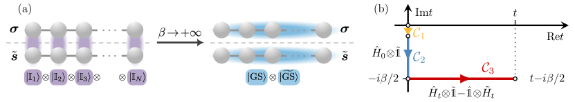
Figure 1: (a) Schematic illustration of the thermofield representation of the state of an ensemble of spins. In this picture, the maximally mixed state ($T=+\infty$) corresponds to a product of locally pairwise maximally entangled Bell states, which could be captured by a mean-field factor; the pure state ($T=0$) corresponds to two copies of the ground-state wave function, whose correlations may be faithfully encoded by a neural-network Ansatz. (b) Time integration contour. The state is first evolved in imaginary time with $\hat{H}_{0}$ till $-i\beta/2$ (see Eq. (2)), initially with an implicit solver ($\mathcal{C}_{1}$) and then with SR ($\mathcal{C}_{2}$). Real-time evolution of the thermal state under $\hat{H}_{t}^{\mathrm{th}}$ (see Eq. (4)) is then performed via t-VMC ($\mathcal{C}_{3}$).

In this Letter, we describe a variational method for performing real-time dynamics of thermal states, bringing together NQS and the concept of thermofield dynamics Takahashi and Umezawa (1975); Suzuki (1985). Our approach relies on the preparation of an NQS in a thermal-vacuum state through imaginary time evolution from a maximally mixed state, using a new approach to accurately time-evolve high-temperature states. We use our technique to simulate the transverse-field Ising model, subject to the sudden effect of a symmetry-breaking longitudinal field. Our approach allows us to study sizes beyond reach within exact simulations.

Thermofield dynamics.— Thermofield dynamics Takahashi and Umezawa (1975); Suzuki (1985) is a general approach to model the behavior of thermal quantum systems, with applications in cosmology Israel (1976), condensed matter Suzuki (1985) and, more recently, quantum chemistry Harsha et al. (2019a); Shushkov and Miller (2019); Harsha et al. (2019b, 2020) and quantum information Chapman et al. (2019), or to prepare thermal quantum states on quantum devices Lee et al. (2022); Zhu et al. (2020). The underlying idea is to interpret the expectation value $\expectationvalue{\smash{\hat{O}}}_{\beta}$ of an observable $\hat{O}$ on a thermal state at inverse temperature $\beta=(k_{B}T)^{-1}$ as that on a pure state belonging to a doubled Hilbert space $\mathcal{H}\otimes\tilde{\mathcal{H}}$:

$$\expectationvalue{\smash{\hat{O}}}_{\beta}=\frac{\Tr[\hat{O}e^{-\beta\hat{H}_{0}}\bigr{]}}{\Tr[e^{-\beta\hat{H}_{0}}\bigr{]}}=\frac{\matrixelement{\Omega(\beta)}{\hat{O}\otimes\tilde{\mathds{1}}}{\Omega(\beta)}}{\innerproduct{\Omega(\beta)}{\Omega(\beta)}},$$ (1)

where the ancillary space is indicated by a tilde and where the so-called thermal vacuum,

$$\ket{\Omega(\beta)}=e^{-\frac{\beta}{2}\hat{H}_{0}\otimes\tilde{\mathds{1}}}\ket{\mathbb{I}},$$ (2)

corresponds to the imaginary-time evolution for a time $\beta/2$ of the identity state

$$\ket{\mathbb{I}}=\frac{1}{\sqrt{\absolutevalue{\mathcal{H}}}}\sum_{n,\tilde{n}}\ket{n,\tilde{n}}\delta_{n,\tilde{n}},$$ (3)

for any orthonormal basis $\{\ket{n}\}_{n=1}^{\lvert\mathcal{H}\rvert}$ of the physical Hilbert space $\mathcal{H}$. In Eq. (3) the physical and thermofield degrees of freedom are pairwise maximally entangled at infinite temperature. More generally, we refer to the thermal vacuum, or its time-evolved state, as a thermofield thermal state $\ket{\Psi(\beta,t)}$, such that $\ket{\Psi(\beta,0)}\equiv\ket{\Omega(\beta)}$. Alternatively, the state can be denoted $\ket{\sqrt{\rho}(\beta,t)}$ since it corresponds to the purification of $\sqrt{\hat{\rho}}$. It then follows from the quadratic form of Eq. (1) that observable expectations are ensured to be taken on a physical (positive semi-definite) density matrix. This is in contrast, for example, with states represented in the POVM formalism Carrasquilla et al. (2019, 2021); Luo et al. (2022); Reh et al. (2021). It is also worth noticing that, in principle, this class of operators encompasses all positive semi-definite trace-class operators, not only thermal ones.

While Eq. (2) governs the imaginary-time evolution of the state of the system from the infinite-temperature state $\ket{\Psi(0,0)}=\ket{\Omega(0)}\equiv\ket{\mathbb{I}}$, the real-time dynamics is translated into the following Schrödinger equation for the thermofield thermal state Gyamfi (2020):

$$\partial_{t}\ket{\Psi(\beta,t)} =-i(\hat{H}\otimes\tilde{\mathds{1}}-\hat{\mathds{1}}\otimes\tilde{H})\ket{\Psi(\beta,t)}$$

$$\equiv-i\hat{H}^{\mathrm{th}}\ket{\Psi(\beta,t)},$$ (4)

where the effect of tilde conjugation on operators depends upon the quantum statistics of the particles under investigation Arimitsu and Umezawa (1985); Harsha et al. (2019a). We refer to the Supplemental Material  for details on the connection to the density-matrix formalism.

Neural thermofield states.— We consider a physical system consisting of spin-$1/2$ particles. In the $S_{z}$ basis, its neural thermofield state (NTFS) can be expressed as

$$\ket{\Psi_{{\bf\it\theta}}(\beta,t)}=\sum_{{\bf\it\sigma},\tilde{{\bf\it s}}}\psi_{{\bf\it\theta}(\beta,t)}({\bf\it\sigma},\tilde{{\bf\it s}})\ket{{\bf\it\sigma},\tilde{{\bf\it s}}}.$$ (5)

Here, ${\bf\it\sigma},\tilde{{\bf\it s}}\in\{\uparrow,\downarrow\}^{N}$ respectively denote the physical and auxiliary (thermofield) spin configurations, ${\bf\it\theta}$ the set of variational parameters, and $\psi_{{\bf\it\theta}}$ the corresponding Ansatz wave function. The minimal requirement for Eq. (5) to represent a viable neural thermofield state is to be able to represent the identity state exactly for a suitable choice of initial parameters, i.e.

$$\psi_{{\bf\it\theta}(\beta=0)}({\bf\it\sigma},\tilde{{\bf\it s}})\propto\innerproduct{{\bf\it\sigma}}{\tilde{{\bf\it s}}}.$$ (6)

While such a construction is not obvious in general, we here focus on two implementations: a restricted Boltzmann machine operator (RBMO) Nomura et al. (2021); Carleo and Troyer (2017), and a novel autoregressive recurrent neural-network operator, which we dub ARNNO. The autoregressive property of the latter gives access to uncorrelated direct sampling from the Born distribution, dispensing from Markov-chain techniques, which has shown valuable in the study of closed quantum systems Sharir et al. (2020); Hibat-Allah et al. (2020); Wu et al. (2022). A third general implementation, applicable to arbitrary neural-network architectures, is included in the Supplemental Material Note (1), along with details about the architectures and initialization used in the numerical experiments. We next describe how to prepare the NQS in the maximally mixed state exactly and how to evolve them both in imaginary and real-time.

Variational thermal-state preparation— The overall procedure for carrying out the real-time evolution of a thermal state in the thermofield picture is depicted in Fig. 1 (b). In both real and imaginary time, one can use the time-dependent variational principle (TDVP) Yuan et al. (2019); Broeckhove et al. (1988). In conjunction with Monte Carlo estimates for the expectation values, imaginary-time TDVP reduces to stochastic reconfiguration (SR) Sorella (1998). A major obstacle prevents one from preparing the thermal-vacuum state via SR ($\mathcal{C}_{1}$). Indeed, in the $S_{z}$ basis, the gradients of the expectation value of the time-propagator (also called “forces” Vicentini et al. (2022b)) vanish at $\beta=0$ when Monte Carlo estimates are used. On the other hand, current implicit methods Sinibaldi et al. (2023) have fidelity gradients that are dominated by probability amplitudes with large magnitudes, and, therefore, cannot depart from the infinite-temperature state. To circumvent these issues, it was proposed to add noise to the parameters of the Ansatz Nomura et al. (2021) at the cost of introducing uncontrollable errors and bias in the imaginary time evolution, eventually rendering the method unreliable in studying real-time evolution. We propose two solutions to this obstacle. Our first approach is based on the observation that the above-mentioned bias occurs due to the presence of many zeros in the maximally-entangled identity state. The zeros in the wave function can be lifted by applying a Hadamard rotation to the auxiliary thermofield doubled spins: $\left(\ket{00}+\ket{11}\right)^{\otimes N}\to\left(\ket{00}+\ket{01}+\ket{10}-\ket{11}\right)^{\otimes N}$. The rotated basis resolves the bias such that standard SR can be used to depart from $\beta=0$ in $\mathcal{C}_{1}$. Our second approach is to introduce a novel implicit variational method dubbed (projected Imaginary Time Evolution, p-ITE), which we apply to start the imaginary-time evolution in $\mathcal{C}_{1}$ till the gradient signal can be accurately resolved. Therefore, we resort to an implicit formulation of TDVP Gutiérrez and Mendl (2022); Sinibaldi et al. (2023) and enforce a finite sample density on zero-amplitude states responsible for biasing the forces by means of self-normalized importance sampling using the following suitable prior distribution from which we can sample directly:

$$q({\bf\it S})=\mathcal{N}\sum_{{\bf\it S}^{\prime}}\lvert\innerproduct{{\bf\it S}^{\prime}}{\mathbb{I}}\rvert^{2}f\bigl{(}{\bf\it S}^{\prime},{\bf\it S}\bigr{)},$$ (7)

where ${\bf\it S}=({\bf\it\sigma},\tilde{{\bf\it s}})$, $\mathcal{N}$ is a normalization constant, and $f$ is a suitably chosen convolutional kernel. Details about the estimators are given in the Supplemental Material Note (1).

Neural thermofield dynamics: real-time evolution— For section $\mathcal{C}_{3}$ in Fig. 1, we can now carry out the real-time evolution as if we are handling a closed quantum system in the enlarged Hilbert space, subject to the thermofield Hamiltonian in Eq. (4). In conjunction with Monte Carlo, TDVP in this case reduces to the time-dependent Variational Monte Carlo (t-VMC) Carleo et al. (2012, 2017).

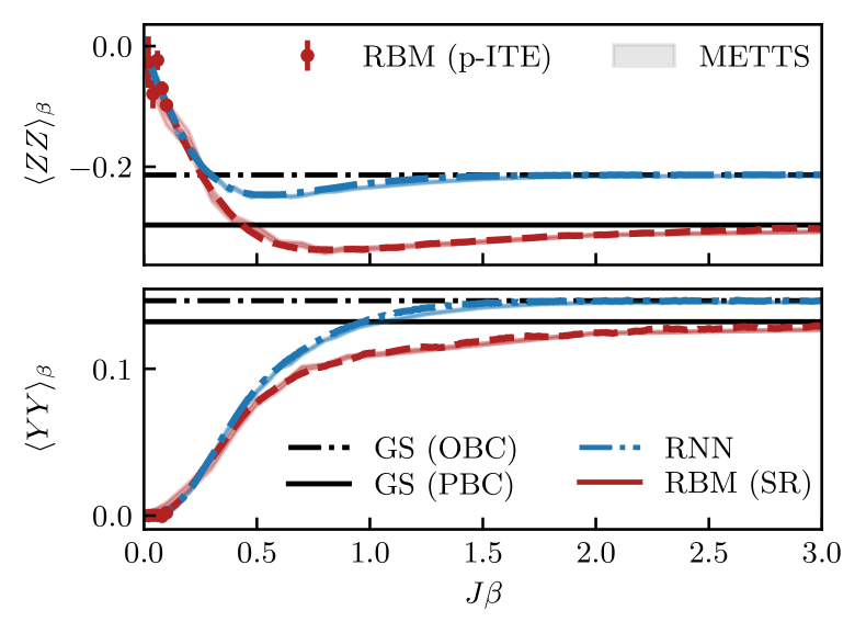
Figure 2: Thermal observables evolution as a function of $\beta$, for a $4{\times}4$ lattice at the critical point. OBC was used for the ARNNO, while PBC was used for the RBMO, along with p-ITE for the initial dynamics. METTS predictions (with $3\sigma$ bands, 10k samples) and ground-state (GS) values ($\beta\to\infty$) are added for comparison. For the RBMO, observables in the p-ITE temperature regime are estimated via standard local Monte Carlo sampling and thus have higher variance than the sampling scheme used in the actual p-ITE propagation. Operators are evaluated on neighbouring sites.

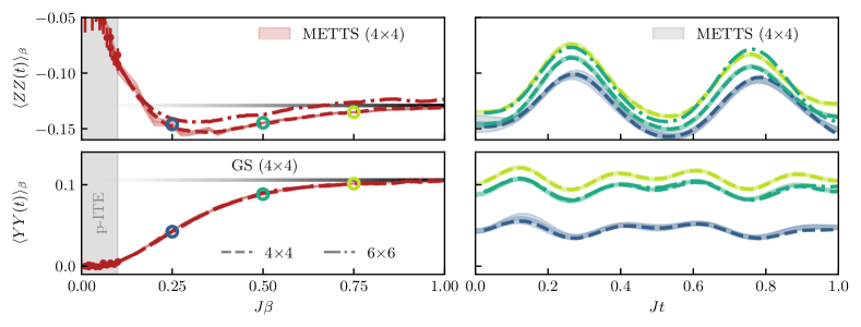
Figure 3: Thermal observables evolution as a function of $\beta$ (left) and real time $t$ (right) for a $4{\times}4$ spin lattice. METTS predictions (with $3\sigma$ bands, 10k samples) and ground-state (GS) values ($\beta\to\infty$) are added for comparison. We also show the results at $\beta=1/2$ for a $6{\times}6$ lattice, which are hard to distinguish from the $4{\times}4$ results for the $YY$ operator. For the RBMO, observables in the p-ITE temperature regime are estimated via standard local Monte Carlo sampling and thus have higher variance than the sampling scheme used in the actual p-ITE propagation. Operators are evaluated on neighbouring sites.

Transverse- and longitudinal-field Ising model.— We first consider the generalized transverse-field Ising model, as described by the Hamiltonian

$$\hat{H}(h_{T},h_{L}) =J\sum_{\left<i,j\right>}\hat{\sigma}_{i}^{z}\hat{\sigma}_{j}^{z}-h_{T}\sum_{i}\hat{\sigma}_{i}^{x}+h_{L}\sum_{i}\hat{\sigma}_{i}^{z},$$ (8)

where $J$ denotes the nearest-neighbor interaction strength, and $h_{T}$ and $h_{L}$ are the transverse and longitudinal fields, respectively. At zero temperature and zero longitudinal field, this system exhibits a second-order phase transition at $h_{c}=3.04438(2)J$ Blöte and Deng (2002).

We first simulate thermal states of the initial critical Hamiltonian $\hat{H}_{0}=\hat{H}(h_{c},0)$ and demonstrate that our techniques can accurately model the thermal-state preparation, even at the critical point. In Fig. 2 we compare our simulations against exact METTS predictions  for a 2D system using both the ARNNO and RBMO thermal states (see Supplemental Material Note (1) for details about the METTS benchmark).

At the critical point, the system is known to exhibit singular magnetic susceptibility in the thermodynamic limit along the longitudinal direction Stinchcombe (1973). We probe the dynamics in this direction through the $ZZ$ operator. This quantifies the density of topological defects in the system and is known as a meaningful probe to interesting critical universal phenomena such as the Kibble-Zurek mechanism Puebla et al. (2019); Donatella et al. (2023). We also measure the $YY$ operator, showing the technique also proves accurate when dealing with off-diagonal operators. In both cases, the difference with METTS is hardly visible, thereby validating the accuracy of our method in reconstructing thermal states over a wide range of temperatures, even when the underlying density matrices are non-trivial. In particular, one observes that the Ansatz correctly interpolates between the infinite-T maximally mixed state and the closed-system ground-state asymptotics.

Next, we carry out the real-time evolution of a thermal state. To this aim, we first prepare the thermal state of the Hamiltonian $\hat{H}_{0}=\hat{H}(1.5h_{c},0)$ at several temperatures of interest. The system is subsequently evolved according to $\hat{H}_{t}=\hat{H}(1.5h_{c},J)$, simulating the sudden switching on of a parity-breaking longitudinal field. The latter is obtained by evolving the finite-temperature (doubled) state with the thermofield Hamiltonian $\hat{H}_{t}^{\mathrm{th}}$ defined in accordance with Eq. (4). In Fig. 3, we show the results for 2D lattices of size $4{\times}4$ and $6{\times}6$, respectively (see Supplementary Material Note (1) for simulations on a 1D chain of $10$ spins, and a comparison with exact diagonalization). Our simulations faithfully reproduce the oscillations induced by the longitudinal external field onto the system, originally in an orthogonally polarized paramagnetic phase. For these experiments, we use the RBMO architecture since it is holomorphic and therefore results in stable time evolution with tVMC. For ARNNO, implicit time evolution techniques such as the one introduced in Ref. Sinibaldi et al. (2023) prove valuable. We also show predictions from METTS and the corresponding variance. We conclude that our method can reliably capture real-time dynamics for a wide range of temperatures. Especially as the temperature decreases, where our results become increasingly accurate since the variance on the Monte Carlo estimators in tVMC decreases, thereby requiring fewer samples to obtain a similar accuracy in the energy gradients.

Discussion and outlook.— We introduced the framework of thermofield dynamics to capture the real-time evolution of thermal ensembles using neural network quantum states. We demonstrated its accuracy and scalability on the Ising model with a longitudinal and transverse field. First, we solve the problem of accurately preparing a neural density operator at a given temperature. We do this by introducing both novel autoregressive neural network operators (ARNNO) and a stable implicit imaginary-time evolution technique (p-ITE) that allows one to cool down generic neural density operators. Unlike the POVM-based formalism, our variational thermal states are guaranteed to be positive semi-definite, and, therefore, physical. Within the thermofield formalism, we perform real-time evolution of these thermal neural density operators and are able to scale our simulations beyond system sizes accessible with exact methods. Since the generality of our approach, in principle, allows one to build neural density operators from any neural quantum architecture, we foresee many extensions. This should prove useful in simulating electronic systems Nys and Carleo (2022), with application in quantum chemistry, material science, and condensed matter; and may result in a better understanding of temperature dependence of analog quantum simulators and the influence of environmental noise on digital quantum devices.

Supplemental Material to “Real-time quantum dynamics of thermal states with neural thermofields”

I Thermal state architectures

As mentioned in the main text, any thermal Ansatz must be able to represent the infinite temperature state (the identity state in the thermofield formalism) exactly. Below, we introduce three methods to accomplish this goal, starting with a generic Ansatz, eventually leading to the ARNNO and RBMO ansatzes used in the results section of the main text.

I.1 Generic neural-network architecture

One can encode the structure of the identity state into a mean-field factor, thereby entirely lifting any restriction on the architecture of the model. Therefore, we realize that the identity state is a product state with maximally entangled physical-thermofield spin pairs. A possible construction therefore reads

$$\ket{\Omega_{{\bf\it\theta}}(\beta)}=\sum_{{\bf\it\sigma},\tilde{{\bf\it s}}}\psi_{{\bf\it\theta}(\beta)}({\bf\it\sigma},\tilde{{\bf\it s}})\bigotimes_{i=1}^{N}\sqrt{p_{{\bf\it\theta}(\beta)}^{\mathrm{MF}}(\sigma_{i},\tilde{s}_{i})}\ket{\sigma_{i},\tilde{s}_{i}},$$ (S1)

where $p_{{\bf\it\theta}}^{\mathrm{MF}}$ denotes the mean-field factor. As discussed in the main text, there is some freedom in defining this state. However, in the $\hat{S}_{z}$ basis, the identity $\bigotimes_{i=1}^{N}\ket{\mathbb{I}_{i}}$ can be represented exactly by the separable mean-field factor, by ensuring

$$\psi_{{\bf\it\theta}(\beta=0)}({\bf\it\sigma},\tilde{{\bf\it s}})=\text{cst.},\quad p_{{\bf\it\theta}(\beta=0)}^{\mathrm{MF}}(\sigma,\tilde{s})\propto\innerproduct{\sigma}{\tilde{s}}$$ (S2)

at $\beta=0$. In this scenario, the architecture of the neural thermofield state of Eq. (S1) becomes clear. The mean-field separable factor captures the initial infinite-temperature structure while the neural network encodes both “local” correlations between physical and auxiliary spins and those between distant spins, which build up as the state is evolved in imaginary time to a finite inverse temperature $\beta$. This is schematically depicted in Fig. 1 (a) in the main text.

I.2 ARNNO: ARNN architecture

We introduce two possible ARNNO architectures: first, we start in the $S_{z}$ basis by turning the existing RNN architecture from Ref. Hibat-Allah et al. (2020) into a thermal state. We point out that this ansatz would result in zero gradients in the infinite temperature state, and introduce a solution to this problem by representing the thermofield spins in a rotated basis.

I.2.1 In the $(S_{z},\tilde{S}_{z})$ basis

The NTFS in Eq. (S1) of the main text can be implemented as a recurrent neural network in the $S_{z}$ with the following spin-pair autoregressive architecture:

$$\psi_{{\bf\it\theta}}({\bf\it S}) =\prod_{i=1}^{N}\psi^{(i)}_{{\bf\it\theta}}(S_{i}|{\bf\it S}_{<i}),$$ (S3)

where we have introduced the notation $S_{i}=(\sigma_{i},\tilde{s}_{i})$. Furthermore, we decompose $\psi^{(i)}_{{\bf\it\theta}}=\sqrt{p_{{\bf\it\theta}}^{\mbox{\tiny$(i)$}}}e^{i\phi_{{\bf\it\theta}}^{\mbox{\tiny$(i)$}}}$. The Born distribution inherits this structure and samples can be drawn by iteratively producing pairs of physical-auxiliary spin configurations from the first to the last site without the need for a Markov chain. The mean-field factor at every site is then simply chosen as $\sqrt{p^{\mathrm{MF}}}(\sigma,\tilde{s})=\alpha^{2}\innerproduct{\sigma}{\tilde{s}}$, where $\alpha$ is a real variational parameter. By design, this factor is compatible with the autoregressive property. In sum, the thermofield identity state can be represented purely through a careful design of the output layers at every site.

I.2.2 In the $(S_{z},\tilde{S}_{x})$ basis

The above implementation suffers from zero gradients at the initial $\beta=0$ and must thus be first evolved through the p-ITE method described in the main text. This stems from the presence of exact zeros in the identity-state wave function. Alternatively, one can perform a Hadamard rotation $\hat{\mathds{1}}\otimes(\tilde{\sigma}^{x}+\tilde{\sigma}^{z})/\sqrt{2}$ of the local computational basis. This transformation only acts on the thermofield space and therefore has no incidence on imaginary-time evolution, which only involves the action of physical operators.

Let us consider

$$\ket{0}=\ket{0\tilde{-}},\quad\ket{1}=\ket{0\tilde{+}},\quad\ket{2}=\ket{1\tilde{-}},\quad\ket{3}=\ket{1\tilde{+}};$$ (S4)

as the computational basis of this local space of physical-thermofield pairs. Then, one needs to impose

$$\innerproduct{0,\tilde{1}}{\psi_{{\bf\it\theta}(0)}}\propto\innerproduct{0,\tilde{+}}{\psi_{{\bf\it\theta}(0)}}-\innerproduct{0\tilde{-}}{\psi_{{\bf\it\theta}(0)}} =0,$$ (S5)

$$\innerproduct{1,\tilde{0}}{\psi_{{\bf\it\theta}(0)}}\propto\innerproduct{1,\tilde{+}}{\psi_{{\bf\it\theta}(0)}}+\innerproduct{1\tilde{-}}{\psi_{{\bf\it\theta}(0)}} =0;$$ (S6)

and

$$\innerproduct{0,\tilde{0}}{\psi_{{\bf\it\theta}(0)}}\propto\innerproduct{0,\tilde{+}}{\psi_{{\bf\it\theta}(0)}}+\innerproduct{0\tilde{-}}{\psi_{{\bf\it\theta}(0)}} =C,$$ (S7)

$$\innerproduct{1,\tilde{1}}{\psi_{{\bf\it\theta}(0)}}\propto\innerproduct{1,\tilde{+}}{\psi_{{\bf\it\theta}(0)}}-\innerproduct{1\tilde{-}}{\psi_{{\bf\it\theta}(0)}} =C.$$ (S8)

In the above-defined basis, we investigate how such a state can be constructed in the form of Eq. (S3). First, we defined the normalized probability $p^{(i)}$ based on the unnormalized probability vector $\tilde{{\bf\it p}}^{(i)}$ in the local basis,

$$\begin{gathered}\ln p_{{\bf\it\theta}}^{\mbox{\tiny$(i)$}}=\mathrm{L}\Sigma\mathrm{E}(\ln\tilde{{\bf\it p}}_{{\bf\it\theta}}^{\mbox{\tiny$(i)$}}),\end{gathered}$$ (S9)

where the logsumexp ($\mathrm{L}\Sigma\mathrm{E}$) sums over the 4-dimensional local Hilbert space basis. We now aim to construct the unnormalized probabilities and phases such that

$$\ln\tilde{{\bf\it p}}_{{\bf\it\theta}}^{\mbox{\tiny$(i)$}} =[\gamma_{i},\gamma_{i},\gamma_{i},\gamma_{i}],$$ (S10)

$$\tilde{{\bf\it\phi}}_{{\bf\it\theta}}^{\mbox{\tiny$(i)$}} =[\delta_{i},\delta_{i},\delta_{i}\pm\pi,\delta_{i}].$$ (S11)

In an autoregressive NQS, the amplitudes and phases are obtained as

$$\ln\tilde{{\bf\it p}}_{{\bf\it\theta}}^{\mbox{\tiny$(i)$}}=\mathbf{W}_{\mathrm{amp}}{\bf\it h}^{\mbox{\tiny$(i)$}}+{\bf\it b}_{\mathrm{amp}},$$ (S12)

and

$${\bf\it\phi}_{{\bf\it\theta}}^{\mbox{\tiny$(i)$}}=\pi\left(\mathbf{W}_{\mathrm{ph}}{\bf\it h}^{\mbox{\tiny$(i)$}}+{\bf\it b}_{\mathrm{ph}}\right),$$ (S13)

where

$${\bf\it h}^{{\mbox{\tiny$(i)$}}}=\mathrm{RNN}\bigl{(}\{S_{j}\}_{j\to i};\{{\bf\it h}^{{\mbox{\tiny$(j)$}}}\}_{j\rightarrow i}\bigr{)}$$ (S14)

is the hidden vector at site $i$. Here, ${\bf\it h}^{\mbox{\tiny$(i)$}}\in\mathbb{R}^{P_{h}}$, ${\bf\it b}_{\mathrm{amp}},{\bf\it b}_{\mathrm{ph}}\in\mathbb{R}^{d^{2}}$, $\mathbf{W}_{\mathrm{amp}},\mathbf{W}_{\mathrm{ph}}\in\mathbb{R}^{d^{2}\times P_{h}}$. For reference, the RNN cell used in the main text is an LSTM cell.

In practice, the above identity-state requirements can be fulfilled by generating initial random parameters as

$$\begin{gathered}\mathbf{W}_{\mathrm{amp}}(\beta=0)=\mathbf{0},\quad\mathbf{W}_{\mathrm{amp}}(\beta=0)=\mathbf{0},\\ {\bf\it b}_{\mathrm{amp}}(\beta=0)=x{\bf\it 1},\quad x\sim\mathcal{N}(0,\sigma),\\ \mathbf{b}_{\mathrm{ph}}(\beta=0)=(y,y,y-1,y),\quad y\sim\mathcal{N}(0,\sigma);\end{gathered}$$ (S15)

where we set $\sigma=10^{-2}$.

This neural quantum state does not suffer from zero initial gradients and can thus be evolved in imaginary time with stochastic reconfiguration from $\beta=0$. However, when performing real-time evolution, the thermal Hamiltonian must be partially rotated $\hat{H}^{\mathrm{th}}\mapsto(\hat{\mathds{1}}\otimes\tilde{\mathrm{H}}\mathrm{ad}_{N})\hat{H}^{\mathrm{th}}(\hat{\mathds{1}}\otimes\tilde{\mathrm{H}}\mathrm{ad}_{N})$, where

$$\tilde{\mathrm{H}}\mathrm{ad}_{N}=\bigotimes_{i=1}^{N}(\tilde{\sigma}_{i}^{x}+\tilde{\sigma}_{i}^{z})/\sqrt{2}$$ (S16)

denotes the Hadamard rotation operated on the auxiliary degrees of freedom.

I.3 RBM architecture

An RBM thermal state can be obtained as

$$\ln\psi_{{\bf\it\theta}}({\bf\it\sigma},\tilde{{\bf\it s}}) =\sum_{i}(a_{i}\sigma_{i}+a^{\prime}_{i}\tilde{s}_{i})$$ (S17)

$$+\sum_{m}\ln\cosh\Bigl(b_{m}+\sum_{j}W_{mj}\sigma_{j}+\sum_{j}W^{\prime}_{mj}\tilde{s}_{j}\Bigr{missing}).$$

In order to produce the initial identity state, the parameters are initialized as

$$a_{i}=a^{\prime}_{i}=b_{i}=0,\quad W_{ij}=-W^{\prime}_{ij}=\frac{i\pi}{4}\delta_{i,j}.$$ (S18)

This yields $\ket{\psi_{{\bf\it\theta}}(\beta=0)}\propto\bigotimes_{i}(\ket{\smash{\uparrow\tilde{\uparrow}}}_{i}+\ket{\smash{\downarrow\tilde{\downarrow}}}_{i})$, i.e. the identity state. This initialization is slightly different from that used in Ref. Nomura et al. (2021) and allows working in the $S_{z}$ basis for both the physical and auxiliary space, which considerably simplifies real-time dynamics.

This too yields an Ansatz of the form of Eq. (5). However, contrary to that of the previous subsection, this architecture suffers from exact zero gradients at $\beta=0$.

II projected Imaginary Time Evolution (p-ITE)

This method consists of updating the variational parameters of the wave function to minimize the infidelity,

$${\bf\it\theta}(\beta+\mathrm{d}\beta)=\operatorname*{arg\,min}_{{\bf\it\eta}}\mathcal{I}\bigl{(}\ket{\psi_{{\bf\it\eta}}},\hat{\Pi}\ket{\psi_{{\bf\it\theta}(\beta)}}\bigr{)},$$ (S19)

where $\hat{\Pi}=e^{-\frac{\mathrm{d}\beta}{2}\hat{H}_{0}\otimes\tilde{\mathds{1}}}$ is the imaginary-time propagator. This optimization can be done via stochastic gradient descent. In principle, the infidelity and gradients may be estimated by only sampling from $\lvert\psi_{{\bf\it\eta}}\rvert^{2}$, as previously proposed for real-time evolution Donatella et al. (2023). However, this approach is unable to lift the exact zeros of the wave function. Furthermore, traditional stochastic reconfiguration is biased whenever the state contains vanishing amplitudes for basis states with important energy-gradient contributions Sinibaldi et al. (2023), and is unable to lift the exact zeros of the wave function.

We continue by estimating the various terms of the fidelity between two states $\ket{\psi}$ and $\ket{\phi}$:

$$\mathcal{F}\bigl{(}\ket{\psi},\ket{\phi}\bigr{)}=\Re{AB},$$ (S20)

with

$$A =\innerproduct{\phi}{\psi}/\innerproduct{\phi}{\phi}=\underset{{\bf\it S}\sim q}{\mathbb{E}}\left[w({\bf\it S};\phi)\frac{\psi({\bf\it S})}{\phi({\bf\it S})}\right]/\underset{{\bf\it S}\sim q}{\mathbb{E}}\left[w({\bf\it S};\phi)\right],$$

$$B =\innerproduct{\psi}{\phi}/\innerproduct{\psi}{\psi}=\underset{{\bf\it S}\sim q}{\mathbb{E}}\left[w({\bf\it S};\psi)\frac{\phi({\bf\it S})}{\psi({\bf\it S})}\right]/\underset{{\bf\it S}\sim q}{\mathbb{E}}\left[w({\bf\it S};\psi)\right],$$ (S21)

where $w({\bf\it S};\varphi):=\lvert\varphi({\bf\it S})\rvert^{2}/q({\bf\it S})$ and where, as in the main text, ${\bf\it S}:=({\bf\it\sigma},\tilde{{\bf\it s}})$ was used to alleviate notations. Specifically, if we aim to evolve a variational state for a time $\mathrm{d}t$ from $\ket{\psi_{{\bf\it\theta}}(t)}$ into $\hat{\Pi}\ket{\psi_{{\bf\it\theta}}(t)}$ with a propagator $\hat{\Pi}$, we use the above definitions upon identifying $\ket{\psi}\equiv\ket{\psi_{{\bf\it\theta}}(t)}$ and $\ket{\phi}\equiv\hat{\Pi}\ket{\psi_{{\bf\it\theta}}(t)}$. Hence, in our estimator, gradients of $\psi_{{\bf\it\theta}}$ with respect to the parameters ${\bf\it\theta}$ only need to be computed on the samples ${\bf\it S}$.

Even the standard implicit formulation of SR yields biased imaginary time trajectories, as mentioned in the main text. Therefore, we introduce the following suitable prior distribution from which we can sample directly:

$$q({\bf\it S})=\mathcal{N}\sum_{{\bf\it S}^{\prime}}\lvert\innerproduct{{\bf\it S}^{\prime}}{\mathbb{I}}\rvert^{2}f\bigl{(}D({\bf\it S}^{\prime},{\bf\it S})\bigr{)},$$ (S22)

where $\mathcal{N}$ is a normalization constant. Here, the convolutional kernel decays exponentially with the sample Hamming distances $D_{H}({\bf\it S}^{\prime},{\bf\it S}):=\sum_{i}1-\innerproduct{S^{\prime}_{i}}{S_{i}}$ and $f(D)=b^{-D}$ with hyperparameters $b$. The choice of Hamming distance is inspired by the fact that the state deviates from the identity state through powers of $\hat{H}\mathrm{d}t$ where $\hat{H}$ is local and where the importance of the $n$th power decays exponentially for small $\mathrm{d}t$. Importance sampling proves crucial to optimize the infidelity to sufficiently low values. Furthermore, we reduce the variance on the fidelity operator using the covariate technique in the recently introduced p-tVMC approach in Ref. Sinibaldi et al. (2023).

III Thermofield dynamics with tVMC

The real-time evolution of the thermofield state is governed by the Schrödinger equation (4). In variational space, this dynamical equation may be expressed implicitly as

$$\dot{{\bf\it\theta}}=\operatorname*{arg\,min}_{{\bf\it\eta}}\mathcal{D}(\ket{\psi_{{\bf\it\theta}+\mathrm{d}t{\bf\it\eta}}},e^{-i\mathrm{d}t\hat{H}^{\mathrm{th}}}\ket{\psi_{{\bf\it\theta}}}),$$ (S23)

where $\mathcal{D}$ is the Fubini-Study distance. To leading order in $\mathrm{d}t$, this leads to

$$\mathbf{G}\dot{{\bf\it\theta}}=-i{\bf\it F}^{\mathrm{th}},$$ (S24)

where we introduced the quantum geometric tensor (QGT)

$$G_{k,k^{\prime}}=\mathbb{E}\bigl{[}O_{k}^{\star}({\bf\it S})O_{k^{\prime}}({\bf\it S})\bigr{]}-\mathbb{E}\bigl{[}O_{k}^{\star}({\bf\it S})]\mathbb{E}\bigl{[}O_{k^{\prime}}({\bf\it S})\bigr{]},$$ (S25)

with log-derivatives $O_{k}$ and forces given by

$$O_{k}({\bf\it S})=\partial_{\theta_{k}}\ln\psi_{{\bf\it\theta}}({\bf\it S}),$$ (S26)

$$F_{k}^{\mathrm{th}}=\mathbb{E}\bigl{[}O_{k}^{\star}({\bf\it S})E_{\mathrm{loc}}^{\mathrm{th}}({\bf\it S})\bigr{]}-\mathbb{E}\bigl{[}O_{k}^{\star}({\bf\it S})\bigr{]}\mathbb{E}\bigl{[}E_{\mathrm{loc}}^{\mathrm{th}}({\bf\it S})\bigr{]}.$$ (S27)

In the above ${\bf\it S}:=({\bf\it\sigma},\tilde{{\bf\it s}})$ was defined to alleviate notations and expectation values are implicitly taken with respect to the Born distribution $\lvert\psi_{{\bf\it\theta}}\rvert^{2}$.

The local-energy estimator for the thermal Hamiltonian reads

$$E_{\mathrm{loc}}^{\mathrm{th}}({\bf\it\sigma},\tilde{{\bf\it s}})= \sum_{{\bf\it\sigma}^{\prime}}\frac{\psi_{{\bf\it\theta}}({\bf\it\sigma}^{\prime},\tilde{{\bf\it s}})}{\psi_{{\bf\it\theta}}({\bf\it\sigma},\tilde{{\bf\it s}})}\matrixelement{{\bf\it\sigma}}{\hat{H}}{\tilde{{\bf\it\sigma}}^{\prime}}-$$

$$\sum_{\tilde{{\bf\it s}}^{\prime}}\frac{\psi_{{\bf\it\theta}}({\bf\it\sigma},\tilde{{\bf\it s}}^{\prime})}{\psi_{{\bf\it\theta}}({\bf\it\sigma},\tilde{{\bf\it s}})}\matrixelement{\tilde{{\bf\it s}}}{\tilde{H}}{\tilde{{\bf\it s}}^{\prime}}.$$ (S28)

All these quantities can be efficiently estimated by sampling from $\lvert\psi_{{\bf\it\theta}}\rvert^{2}$. The above variational algorithm may be easily adapted in order to properly work with normalized Ansätze by subtracting the variational energy from the thermal Hamiltonian $\hat{H}^{\mathrm{th}}\mapsto\hat{H}^{\mathrm{th}}-E^{\mathrm{th}}_{{\bf\it\theta}}$. Furthermore, subtracting the average energy reduces the variance of the estimators.

IV Thermofield algebra

The thermofield spin-operator $\tilde{\sigma}$ commutes with operators on the physical Hilbert space, and has the matrix elements

$$\matrixelement{\tilde{m}}{\tilde{\sigma}}{\tilde{n}} =\innerproduct{\tilde{m}}{\widetilde{\sigma n}}$$ (S29)

$$=\bra{\tilde{m}}\left(\sum_{\lambda=1}^{\dim\mathcal{H}}\matrixelement{\lambda}{\hat{\sigma}}{n}^{*}\ket{\smash{\tilde{\lambda}}}\right)$$ (S30)

$$=\matrixelement{m}{\hat{\sigma}}{n}^{*}$$ (S31)

where we used Eq. (S33). In other words, we have $\tilde{\sigma}\to\hat{\sigma}^{*}$, or $\tilde{\sigma}^{x}\to\sigma^{x}$, $\tilde{\sigma}^{y}\to-\sigma^{y}$ and $\tilde{\sigma}^{z}\to\sigma^{z}$. See also the Thermo-SU(2) algebra in Ref. Petronilo et al. (2021).

V Connection to the density-matrix approach

The connection is direct through Liouville space, see Ref. Arimitsu and Umezawa (1985); Gyamfi (2020). Let $\mathcal{O}$ denote the space of operators acting on the physical Hilbert space $\mathcal{H}$, the action of any superoperator onto any element of $\mathcal{O}$ can be mapped into the action of an operator onto a Liouville space of superkets $\mathcal{L}$. The isomorphism between $\mathcal{O}$ and $\mathcal{L}$ is given by the action of the bra-flipping linear superoperator $\mathcal{T}$:

$$\mathcal{T}\bigl{[}\outerproduct{\psi}{\phi}\bigr{]}=\ket{\psi}\otimes\widetilde{\ket{\phi}},$$ (S32)

where one has

$$\widetilde{\ket{\phi}}=\sum_{n=1}^{\dim\mathcal{H}}\innerproduct{n}{\phi}^{\star}\ket{\tilde{n}}.$$ (S33)

This specific behavior of the tilding operation ensures that $\mathcal{T}$ be an isomorphism:

$$\bigl{\langle}\mathcal{T}\hat{A},\mathcal{T}\hat{B}\bigr{\rangle}_{\mathcal{L}}\overset{!}{=}\Tr[\hat{A}^{\dagger}\hat{B}\bigr{]}\equiv\bigl{\langle}\hat{A},\hat{B}\bigr{\rangle}_{\mathcal{O}}.$$ (S34)

The transformation of superoperators into operators acting on Liouville space can be derived from the above:

$$\mathcal{T}\bigl{[}\hat{A}\outerproduct{\psi}{\phi}\hat{B}\bigr{]}=\hat{A}\ket{\psi}\otimes\widetilde{\ket{\smash{\hat{B}\phi}}}=\hat{A}\otimes\tilde{B}\ket{\smash{\psi,\tilde{\phi}}},$$ (S35)

which induces some properties on the action of tilde on operators, for instance

$$(\widetilde{\alpha\hat{A}+\beta\hat{B}})\ket{\smash{\tilde{\phi}}} =\widetilde{\ket{\smash{(\alpha\hat{A}+\beta\hat{B})\phi}}}$$

$$=\sum_{n=1}^{\dim\mathcal{H}}\Bigl{(}\alpha^{\star}\matrixelement{n}{\hat{A}}{\phi}^{\star}\ket{\tilde{n}}+\beta^{\star}\matrixelement{n}{\hat{B}}{\phi}^{\star}\ket{\tilde{n}}\Bigr{)}$$

$$=(\alpha^{\star}\tilde{A}+\beta^{\star}\tilde{B})\ket{\smash{\tilde{\phi}}}.$$ (S36)

From these properties, one can translate the action of superoperators from operator space into Liouville space. For instance,

$$\mathcal{T}\Bigl{[}[\hat{H},\makebox[8.61108pt]{${\color[rgb]{.5,.5,.5}\bullet}$}]\outerproduct{\psi}{\phi}\Bigr{]} =\mathcal{T}\Bigl{[}\outerproduct{\smash{\hat{H}\psi}}{\phi}\Bigr{]}-\mathcal{T}\Bigl{[}\outerproduct{\psi}{\smash{\hat{H}\phi}}\Bigr{]}$$

$$=\bigl{(}\hat{H}\otimes\tilde{\mathds{1}}-\hat{\mathds{1}}\otimes\tilde{H}\bigr{)}\ket{\smash{\psi,\tilde{\phi}}},$$ (S37)

where it becomes clear that tilde space simply accounts for the right action of superoperators on any operator belonging to $\mathcal{O}$. This connection has also been laid out in detail recently in Ref. Kothe and Kirton (2023).

VI Numerical details

We use time steps $\mathrm{d}\beta\in\{0.005,0.01\}/2$ for the initial p-ITE evolution up to $\beta=0.1$ ($\mathcal{C}_{1}$), and $\mathrm{d}\beta\in\{10^{-3},10^{-4}\}/2$ for the second imaginary time evolution using SR ($\mathcal{C}_{2}$). We use the Runge-Kutta 2 and 4 for the SR evolution with RBM and ARNNO respectively. For numerical stability, we use the SVD regularization defined in Ref. Medvidović and Sels (2022) with an absolute cutoff $\texttt{atol}\in\{10^{-7},10^{-8}\}$ for the imaginary and real-time evolution. For the p-ITE, SR and tVMC, we use around $16$k, $64$k and $500$k samples respectively. For the $6{\times}6$ lattice, we use an RBM that is symmetrized over the translation group. For clarity, the data in Figs. 2 and 3 in the main text, and Figs. S1 and S2 hereby were smoothed with a moving average window of size 50.

VII Benchmark on 1D spin chain

In the main text, we show predictions of time-dependent thermal observables on a $4{\times}4$ lattice and compare with METTS predictions to validate our approach. Here we also show predictions for a periodic spin chain of $10$ sites and compare with predictions from exact diagonalization (using the exact matrix exponentials in the time evolution and using the full density matrix). The results are shown in Fig. S1 for the observables $ZZ$ and $YY$ as in the main text. These results again suggest an excellent agreement over a wide temperature range, with the most accurate predictions at lower temperatures.

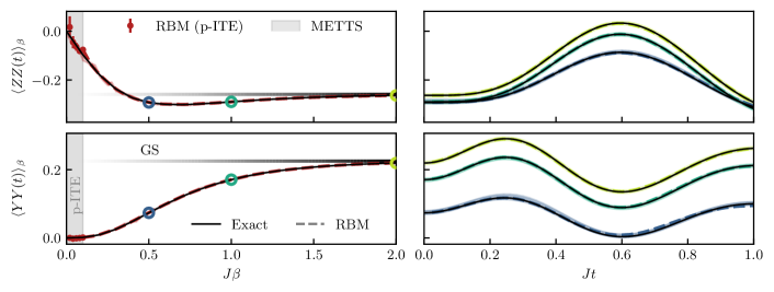
Figure S1: Thermal observables evolution as a function of $\beta$ (left) and real time $t$ (right) for a spin chain of length $10$. The thin black line indicates the exact values. METTS predictions (with $3\sigma$ bands, 10k samples) and ground-state (GS) values ($\beta\to\infty$) are included for comparison. Observables in the p-ITE temperature regime are estimated via standard local Monte Carlo sampling and thus have higher variance than the sampling scheme used in the actual p-ITE propagation. Operators are evaluated on neighboring sites.

VIII Comparison of $4{\times}4$ vs $6{\times}6$

Since we do not have exact predictions available for the time evolution of thermal observables of a $6{\times}6$ lattice, we validate our predictions by matching the energy per site with the $4{\times}4$ lattice in Fig. S2. Although the results of both lattice configurations were produced with different models (see the numerical details section), we obtain an excellent overlap of both thermal energy densities, indicating that our $6{\times}6$ density matrices are trustworthy over the full temperature range.

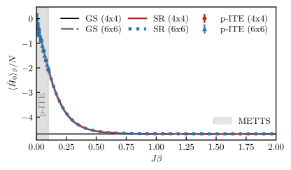
Figure S2: Energy per site as a function of inverse temperature $\beta$ for the $4{\times}4$ and $6{\times}6$ spin torus. Labels are as in Fig. 3 in the main text.

IX Calculating thermodynamic observables with METTS

As a validation of our results on the spin chain of length $10$ and 2D lattice of $4{\times}4$ spins, we compute thermodynamic observables using the minimally entangled thermal states algorithm (METTS) White (2009); Bruognolo et al. (2017); Stoudenmire and White (2010). For an observable $O$ and inverse temperature $\beta$, the METTS algorithm aims to generate a set of samples $\{O_{m}\}_{m}$ whose average approximate the thermal ensemble average

$$\expectationvalue{\smash{\hat{O}}}_{\beta}=\frac{\Tr(e^{-\beta\hat{H}}\hat{O})}{\Tr(e^{-\beta H})}=\lim_{M\to+\infty}\frac{1}{M}\sum_{m=1}^{M}O_{m}.$$

Here, the samples $O_{m}$ are generated via a Markov-chain process as follows:

1. Start from a classical basis state $\ket{n}$.

2. Evolve it up to imaginary time $t=-i\beta/2$

   $$\ket{\phi_{n}(\beta/2)}\propto e^{-\beta\hat{H}/2}\ket{n}.$$

   For this, we use exact state vectors and the Tsitouras 5/4 Runge-Kutta integration method (free 4th order interpolant) Rackauckas and Nie (2017) to solve the differential equation ($\tau=it$)

   $$\frac{\textrm{d}\ket{\phi_{n}(\tau)}}{\textrm{d}\tau}=-\left(\hat{H}_{0}-E_{\tau}\right)\ket{\phi_{n}(\tau)}\,,$$

   where $E_{\tau}=\matrixelement{\phi_{n}(\tau)}{\hat{H}_{0}}{\phi_{n}(\tau)}/\innerproduct{\phi_{n}(\tau)}{\phi_{n}(\tau)}$.

3. Evaluate the observable to obtain the sample

   $$O_{m}\leftarrow\frac{\matrixelement{\phi_{n}(\beta/2)}{\hat{O}}{\phi_{n}(\beta/2)}}{\innerproduct{\phi_{n}(\beta/2)}{\phi_{n}(\beta/2)}}.$$

4. Sample from the Born distribution of $\ket{\phi_{n}(\beta/2)}$ in a chosen basis to obtain the next seed basis state and start again from Step 1.

To reduce the correlations in the Markov chains between subsequent loops, we alternate between measurements in the $Z$ and $X$ basis in Step 4 using Hadamard rotations. This proves crucial, especially at high temperatures. We discard the first $100$ samples of each Markov chain in order to ensure they are properly thermalized.