Appendix: Multi-Robot Informative Path Planning
from Regression with Sparse Gaussian Processes

I Precipitation Dataset Experiments

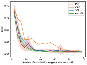
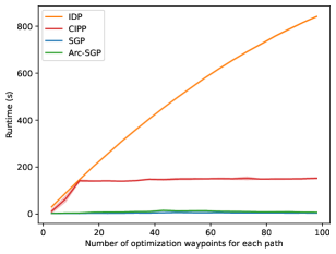
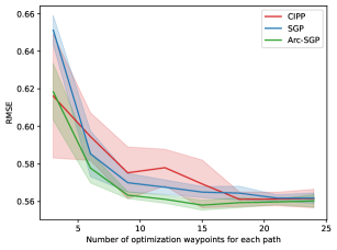
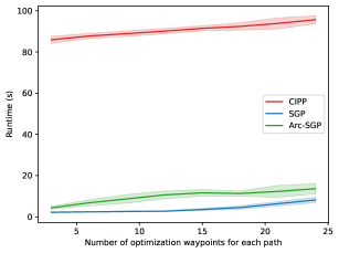
This section presents our results on the precipitation [1] dataset. The precipitation dataset contains daily precipitation data from 167 sensors around Oregon, U.S.A., in 1994. The experimental protocols were the same as the benchmarks presented in the main paper on the other two datasets. Figure 1 and Figure 2 show the single robot and multi-robot IPP results, respectively. We see that the RMSE results saturate to similar scores with fewer number of sensors, but still closely follow the trends of the benchmark results shown in the main paper. In other words, our SGP-based approaches are consistently on par or better than the baselines in terms of RMSE. Additionally, our approaches’ computation time is significantly lower than the baselines.

(a)

(b)

Figure 1: RMSE and runtime results of the IDP, SGP, Arc-SGP, and CIPP approaches on the precipitation dataset.

(a)

(b)

Figure 2: RMSE and runtime results of the SGP, Arc-SGP, and CIPP approaches on the precipitation dataset.

II Efficient Inference and Parameter Estimation

Our SGP based IPP approach is only used to obtain informative path(s). Once we have collected data from the path(s), we can use a full GP to estimate the state of the entire environment. However, even if we use a small number of robots for monitoring, the computational cost of using a GP would eventually become infeasible if we are interested in persistent monitoring of an environment. This is due to the cubic complexity of GPs, which is $\mathcal{O}(r^{3}t^{3})$ when considering data from $r$ robots at $t$ timesteps.

We can address the cubic complexity issue by using the spatio-temporal sparse variational Gaussian process (ST-SVGP, [2]). The approach allows us to use efficient Kalman filtering and smoothing methods to reduce the complexity of the GP to be linear in the number of time steps. Additionally, its use of a sparse approximation reduces the spatial complexity to $\mathcal{O}(u^{3})$, where $u<<rt$ is the number of inducing points used in the ST-SVGP. Therefore, we can efficiently estimate the state of the environment. The approach also allows us to efficiently fit the kernel parameters using maximum likelihood.

III Space-Time Decomposition

When considering multiple robots in spatio-temporal environments, our approach can be further optimized to reduce its computation cost and can be show to have optimal waypoint assignments. When optimizing the paths with $t$ waypoints for $r$ robots, instead of using $rt$ inducing points $\mathbf{X}_{m}\in\mathbb{R}^{r\times t\times(d+1)}$, we can decouple the spatial and temporal inducing points into two sets—spatial and temporal inducing points. The spatial inducing points $\mathbf{X}_{\text{space}}\in\mathbb{R}^{rt\times d}$ are defined only in the $d$-spatial dimensions. The temporal inducing points $\mathbf{X}_{\text{time}}\in\mathbb{R}^{t}$ are defined across the time dimension separately. Also, we assign only one temporal inducing point for the $r$ robots at each time step. This would constrain the $r$ paths to have temporally synchronised waypoints. We then combine the spatial and temporal inducing points by mapping each temporal inducing point to the corresponding $r$ spatial inducing points, forming the spatio-temporal inducing points $\mathbf{X}_{m}\in\mathbb{R}^{r\times t\times(d+1)}$.

The approach allows us to optimize the inducing points across space at each timestep and the timesteps separately. It ensures that there are exactly $r$ inducing points at each time step and also reduces the number of variables that need to be optimized. Specifically, we only have to consider $t$ temporal inducing points, rather than $rt$ inducing points along the temporal dimension. During training, we can use backpropagation to calculate the gradients for the decomposed spatial and temporal inducing points through the spatio-temporal inducing points.

An added advantage of this decomposition is that we can leverage it to prove that the solution paths have optimal waypoint transitions. We do this by setting up an assignment problem that maps the $r$ waypoints at timestep $i$ to the $r$ waypoints at timestep $i+1$. We calculate the assignment costs using pairwise Euclidean distances and get the optimal waypoint transitions for each of the $r$ paths by solving for the assignments [3]. We repeat this procedure for all $t$ timesteps. If the transitions are optimal, the approach would return the original paths, and if not, we would get the optimal solution. The pseudocode of the approach is shown in Algorithm 1, and Figure 3 illustrates our approach.

Figure 3: A schematic illustration of the IPP approach for multiple robots (2 robots). Note that the past training grid is only for visual interpretability and is not used while training the SGP to get the new path.

Input: Inducing points $\mathbf{X}\in\mathbb{R}^{r\times t\times(d+1)}$

Output: Waypoints of paths $\mathbf{X}\in\mathbb{R}^{r\times t\times(d+1)}$

1 for $i\leftarrow 0$ to $t-1$ do

2       $\mathbf{C}=\mathbf{0}^{r\times r}$

3       for $j\leftarrow 1$ to $r$ do

4             for $k\leftarrow 1$ to $r$ do

5                   $\mathbf{C}[j][k]\leftarrow||\mathbf{X}[j,i,:d]-\mathbf{X}[k,i+1,:d]||_{2}$

6            

7      $A=\mathcal{H}(\mathbf{C})$  / / Solve the assignment problem [3]

8       / / Re-index the inducing points at time $i+1$

9       $\mathbf{X}[:,i+1,:d+1]\leftarrow\mathbf{X}[A,i+1,:d+1]$

return $\mathbf{X}$

Algorithm 1 Assignment problem based approach to get optimal waypoint transitions for $r$ paths.

IV IPP with Past Data

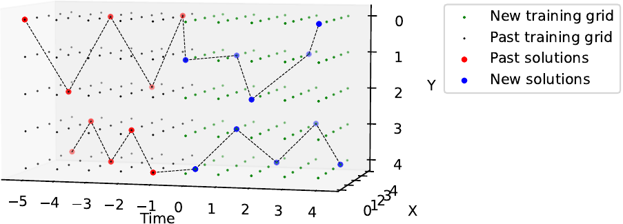
In a real-world scenario, it is possible that a robot has collected data from a sub-region of the environment. In such cases, in addition to updating our kernel parameters, it would be beneficial to explicitly incorporate the data into our path planning approach. We do this by adding more inducing points—auxiliary inducing points—to the SGP in addition to the $m$ inducing points used to get a path with $m$ sampling locations. The auxiliary inducing points are initialized at the locations of the past data samples, and their temporal dimension is set to negative numbers indicating the time that has passed since the corresponding data sample was collected. During training, the auxiliary inducing points are not optimized; only the original $m$ inducing points used to form the path are optimized. Therefore, the approach accounts for past data, including when it was collected, as the points collected further in the past would be less correlated with the SGP’s training data consisting of random samples restricted to the positive timeline. Note that this approach is also suited to address online variants of IPP.

Figure 4: Five points were used as past data (red points). Data collection paths generated using a spatio-temporal kernel function for different distance budgets.

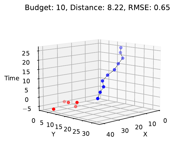
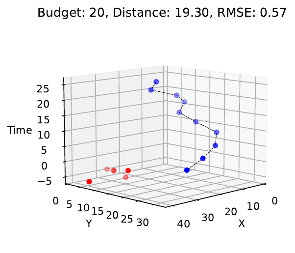
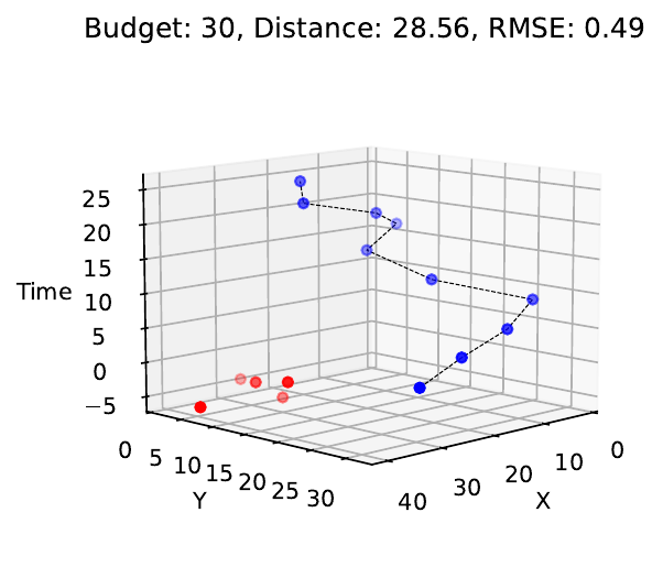
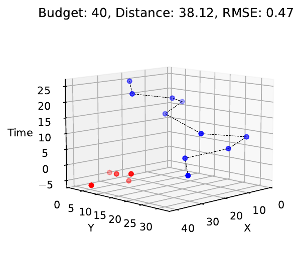
We demonstrate the approach with past data. We used 5 data samples as the past data and generated new informative paths with the distance budgets set to 10, 20, 30, and 40. The results are shown in Figure 4; the red points are the past data samples. As we can see, our new solution paths are shifted to avoid collecting data at the location of the past data. Therefore, our solution paths have lower RMSE scores than those generated without past data information.

V Linear and Non-linear transformations in SGPs

This section show how the SGP sensor placement approach [4] can be generalized to incorporate the expansion and aggregation transformations to address non-point FoV sensor placement, and in turn, non-point FoV informative path planning.

Input: $k_{\theta},\mathcal{V},\Phi$, $s$, $n$, $\gamma$, $T_{\text{exp}}$, $T_{\text{agg}}$

Output: Solution sensor placements $\mathcal{A}\subset\mathcal{V}$, where $|\mathcal{A}|=s$

1

$\mathbf{X}=\{\emptyset\}$ ;

  // Initialize empty set to store SGP training set

2 repeat

       // Draw $n$ random unlabeled locations from the environment

3       $\mathbf{x}\sim\Phi(\mathcal{V})$

4       $\mathbf{X}\leftarrow\mathbf{X}\cup\{\mathbf{x}\}$

5      

6until $|\mathbf{X}|=n$;

$\mathcal{D}=(\mathbf{X},\mathbf{y}=\mathbf{0})$ ;

  // Generate SGP training dataset with $0$ labels

7

$\mathbf{X}_{m}=\text{RandomSubset}(\mathbf{X},s)$ ;

  // Initialize $s$ inducing points at random locations

$\mathbf{X}_{m}\leftarrow\text{RandomTheta}(\mathbf{X}_{m},s)$ ;

  // Add random sampled angles as the rotation parameter of each inducing point

8

$\varphi=\mathcal{SGP}(0,k_{\theta};\mathcal{D},\mathbf{X}_{m})$ ;

  // Initialize a SVGP $\varphi$ with $0$ mean, kernel function $k_{\theta}$, training set $\mathcal{D}$, and inducing points $\mathbf{X}_{m}$

9

10repeat

       $\mathbf{X}_{mp}=T_{\text{exp}}(\mathbf{X}_{m})$ ;

        // Use the expansion transformation $T_{\text{exp}}$ to map the $m$ inducing points $\mathbf{X}_{m}$ in the point parametrization to $mp$ points with FoV parametrization

       $\mathbf{Q}_{nn}=(\mathbf{K}_{n\times mp}T_{\text{agg}})(T_{\text{agg}}^{\top}\mathbf{K}_{mp\times mp}T_{\text{agg}})^{-1}(T_{\text{agg}}^{\top}\mathbf{K}_{mp\times n})$ ;

        // Use the aggregation transformation $T_{\text{agg}}$ to reduce the covariances

       $\mathbf{X}_{m}\leftarrow\mathbf{X}_{m}+\gamma\nabla\mathcal{F}_{\varphi}(\mathbf{Q}_{nn})$ ;

        // Optimize the point parametrized inducing points $\mathbf{X}_{m}$ by maximizing the SVGP’s ELBO $\mathcal{F}_{\varphi}$ using gradient descent (ascent) with a learning rate of $\gamma$. We compute the ELBO using the $\mathbf{Q}_{nn}$ computed above

11      

12until convergence;

return $\mathbf{X}_{m}$

Algorithm 2 Expansion and aggregation transformation based approach for obtaining non-point FoV sensor placements. Here $k_{\theta}$ is the kernel function with parameters learnt from either historical data or expert knowledge, $\Phi$ is a random distribution defined over the bounds of the environment $\mathcal{V}$, $s$ is the number of required sensors, $n$ is the number of random locations used to train the SGP, and $\gamma$ is the SGP learning rate. $T_{\text{exp}}$ and $T_{\text{agg}}$ are the expansion and aggregation transformations, respectively.

Consider a 2-dimensional sensor placement environment. Each of the point parametrized inducing points $\mathbf{X}_{m}\in\mathbb{R}^{m\times 2}$, are mapped to $p$ points ($\mathbf{X}_{m}p\in\mathbb{R}^{mp\times 2}$) using the expansion transformation $T_{\text{exp}}$. This approach scales to any higher dimensional sensor placement environment and can even include additional variables such as the orientation and scale of the sensor/FoV, such as when considering the FoV of a camera on an aerial drone.

The following is an example of the expansion transformation operation written as a function in Python with TensorFlow. The function considers sensor with a FoV shaped as a line with a fixed length.

1 Input: $\mathbf{X}_{m}$, $l$, $p$

2 $x,y,\theta=\text{tf.split}(\mathbf{X}_{m},\text{num\textunderscore or\textunderscore size\textunderscore splits}=3,\text{axis}=1)$

3 $x=\text{tf.squeeze}(x)$

4 $y=\text{tf.squeeze}(y)$

5 $\theta=\text{tf.squeeze}(\theta)$

6 $\mathbf{X}_{m}=\text{tf.linspace}([x,y],[x+l\times\text{tf.cos}(\theta),y+l\times\text{tf.sin}(\theta)],p,\text{axis}=1))$

7 $\mathbf{X}_{m}=\text{tf.transpose}(\mathbf{X}_{m},[2,1,0])$

8 $\mathbf{X}_{m}=\text{tf.reshape}(\mathbf{X}_{m},[-1,2])$

return $\mathbf{X}_{m}$

Algorithm 3 Expansion transformation function (written in Python with TensorFlow [5]) used to map the 2D position ($x,y$) and orientation ($\theta$) to a set of points along a line segment with the origin at the 2D point in the direction of the orientation $\theta$. Here, $\mathbf{X}_{m}$ are the inducing points with the position and orientation parameterization, $l$ is the length of the line along which the mapped points are sampled, and $p$ is the number of points that are sampled along the line.

The aggregation transformation matrix $T_{\text{agg}}\in\mathbb{R}^{mp\times m}$ is populated as follows for $m=3$ and $p=2$ for mean aggregation:

$$T_{\text{agg}}^{\top}=\begin{bmatrix}0.5&0.5&0&0&0&0\\ 0&0&0.5&0.5&0&0\\ 0&0&0&0&0.5&0.5\\ \end{bmatrix}\\ .$$

However, one can even use the 1-dimensional average pooling operation to efficiently apply the aggregation transformation without having to store large aggregation matrices.

References

- [1] C. S. Bretherton, M. Widmann, V. P. Dymnikov, J. M. Wallace, and I. Bladé, “The effective number of spatial degrees of freedom of a time-varying field,” Journal of Climate, vol. 12, no. 7, pp. 1990–2009, 1999.
- [2] O. Hamelijnck, W. J. Wilkinson, N. A. Loppi, A. Solin, and T. Damoulas, “Spatio-Temporal Variational Gaussian Processes,” in Advances in Neural Information Processing Systems, A. Beygelzimer, Y. Dauphin, P. Liang, and J. W. Vaughan, Eds., 2021.
- [3] R. Burkard, M. Dell’Amico, and S. Martello, Assignment Problems: revised reprint. Philadelphia, USA: Society for Industrial and Applied Mathematics, 2012.
- [4] K. Jakkala and S. Akella, “Efficient Sensor Placement from Regression with Sparse Gaussian Processes in Continuous and Discrete Spaces,” 2023, manuscript submitted for publication. [Online]. Available: https://arxiv.org/abs/2303.00028
- [5] M. Abadi, P. Barham, J. Chen, Z. Chen, A. Davis, J. Dean, M. Devin, S. Ghemawat, G. Irving, M. Isard et al., “TensorFlow: A system for large-scale machine learning,” in 12th USENIX Symposium on Operating Systems Design and Implementation (OSDI 16), 2016, pp. 265–283.