A Flexible Online Framework for Projection-Based STFT Phase Retrieval

Abstract

Several recent contributions in the field of iterative STFT phase retrieval have demonstrated that the performance of the classical Griffin-Lim method can be considerably improved upon. By using the same projection operators as Griffin-Lim, but combining them in innovative ways, these approaches achieve better results in terms of both reconstruction quality and required number of iterations, while retaining a similar computational complexity per iteration. However, like Griffin-Lim, these algorithms operate in an offline manner and thus require an entire spectrogram as input, which is an unrealistic requirement for many real-world speech communication applications. We propose to extend RTISI—an existing online (frame-by-frame) variant of the Griffin-Lim algorithm—into a flexible framework that enables straightforward online implementation of any algorithm based on iterative projections. We further employ this framework to implement online variants of the fast Griffin-Lim algorithm, the accelerated Griffin-Lim algorithm, and two algorithms from the optics domain. Evaluation results on speech signals show that, similarly to the offline case, these algorithms can achieve a considerable performance gain compared to RTISI.

Index Terms—  Speech processing, phase retrieval, real-time spectrogram inversion

1 Introduction

Many approaches to digital audio signal processing involve operation in the time-frequency domain, most often by application of the short-time Fourier transform (STFT) on the time-domain signal prior to processing. By definition of the discrete Fourier transform (DFT) and in contrast to the real-valued time domain signal, the resulting time-frequency representation is complex-valued and typically expressed in terms of its magnitude and phase components. While some audio processing systems (e.g. for speech enhancement or source separation) operate directly on the complex-valued STFT representation (the complex spectrogram), or consider both magnitude and phase components, many systems only take the magnitude spectrogram into account. The phase spectrogram which is required for the inverse transformation to the time domain is either taken directly from the input signal (if available) or has to be completely estimated from the magnitude spectrogram. The latter case is often referred to as phase retrieval, phase reconstruction, or spectrogram inversion.

Due to the use of finite overlapping frames, the STFT representation is inherently redundant [1]. This redundancy gives rise to the notion of consistency: A complex spectrogram $\mathbf{X}\in\mathbb{C}^{K{\mkern-2.0mu\times\mkern-2.0mu}L}$ is said to be consistent if and only if it is in the image of the STFT operation, i.e. if it is the result of an STFT on a time domain signal. If this is not the case, transforming a spectrogram to the time domain and back to the time-frequency domain results in a modified spectrogram $\widetilde{\mathbf{X}}\neq\mathbf{X}$. In other words, a complex spectrogram $\mathbf{X}$ is only consistent if $\mathbf{X}=\operatorname{STFT}(\operatorname{iSTFT}(\mathbf{X}))$, where $\operatorname{iSTFT}(\cdot)$ denotes the inverse STFT operation [1, 2].

Iterative projection algorithms are a class of phase retrieval algorithms that make use of consistency by imposing it as a constraint, along with the constraint defined by the known magnitude spectrogram. By iteratively projecting onto sets defined by these two constraints, these algorithms seek an intersection of these two sets: a complex spectrogram that fulfills both constraints by being consistent and having the correct magnitude simultaneously. The basic algorithm used in this context is the Griffin-Lim algorithm (GLA) [3], which was proposed in 1984 and is based on earlier works pertaining to phase retrieval in optics. Several extensions of GLA have been proposed through the years, mainly based on ideas and methods from the optimization field [4, 5], borrowing from advances in optics [6, 7] or based on sparsity and other approximations [8].

Besides the iterative projection paradigm, other approaches to STFT phase retrieval include model-based methods [9, 10], methods based on phase derivatives [11], optimization techniques [12] and recently also methods involving deep neural networks (often in combination with one or more of the above) [13, 14, 15, 16]. In this work, however, we focus solely on projection-based methods.

Many audio applications call for real-time processing (e.g. speech telecommunications or audio broadcast). Whether or not an algorithm is real-time capable depends on specific implementation and hardware details. Notwithstanding that, a fundamental requirement for any real-time algorithm is online and causal operation: it may only process a relatively small chunk of information at a time and may not rely on future information. Real-Time Iterative Spectrogram Inversion (RTISI), proposed by Beauregard et al. [17] and later extended by Zhu et al. [18, 19], is an adaptation of GLA to the online setting. Instead of expecting an entire spectrogram as input like GLA and its relatives, RTISI operates on a single frame at a time. By keeping track of the estimated phase of past frames, RTISI is still able to make use of redundancy, although only in the backward direction relative to the current frame. RTISI-LA [18, 19] relaxes this limitation by introducing “look-ahead” frames, i.e. a certain number of future frames that provide redundancy in the forward direction. Although not strictly causal by definition, RTISI-LA can be implemented causally if the added delay complies with the latency requirements of the application at hand. Other extensions to RTISI include modifications to its initialization scheme and order of frame estimation [20], as well as combinations with other algorithms [21, 22].

While other solutions to online STFT phase retrieval have been proposed [23, 24, 25], RTISI remains a popular choice due to its demonstrated performance and computational efficiency. In this paper, we aim to develop online versions of further iterative algorithms beyond Griffin-Lim. Instead of deriving an online variant for each algorithm specifically, we introduce a more general formulation of RTISI(-LA) that allows quick and straightforward adaptation of any algorithm that is based on the principle of iterative projections.

2 Iterative Phase Retrieval

Iterative projection algorithms transform a given signal by successively enforcing a series of constraints, aiming to converge to a point where all constraints are met. Each constraint is enforced by projecting the signal onto a set defined by that constraint. In the case of STFT phase retrieval, we define two such sets: $\mathcal{A}$ is the set of all complex spectrograms with a given magnitude spectrogram $\mathbf{A}\in\mathbb{R}^{K{\mkern-2.0mu\times\mkern-2.0mu}L}$, and $\mathcal{C}$ is the set of all consistent spectrograms $\mathbf{X}\in\mathbb{C}^{K{\mkern-2.0mu\times\mkern-2.0mu}L}$. The corresponding projection operations can be defined as

$$P_{\mathcal{A}}(\mathbf{X}) =\mathbf{A}e^{j\arg(\mathbf{X})}\,,$$ (1)

$$P_{\mathcal{C}}(\mathbf{X}) =\operatorname{STFT}(\operatorname{iSTFT}(\mathbf{X})\,.$$ (2)

Iterative projection algorithms operate by applying different combinations of $P_{\mathcal{A}}$ and $P_{\mathcal{C}}$ on the input signal in an iterative manner. Starting from an initialization $\mathbf{X}^{0}$, we denote the result of iteration $i$ as $\mathbf{X}^{i}$. In the following, we briefly present the algorithms that are used in this work. Further details are available in [6].

2.1 Griffin-Lim algorithm (GLA)

The classical Griffin-Lim algorithm [3] simply consists of successive applications of both projections:

$$\mathbf{X}^{i+1}=P_{\mathcal{C}}(P_{\mathcal{A}}(\mathbf{X}^{i}))\,.$$ (3)

2.2 Fast Griffin-Lim algorithm (FGLA)

FGLA [4] is similar to GLA but includes an auxiliary sequence $\mathbf{Y}$ that is used to increase the step size taken by the algorithm at each iteration, depending on a parameter $\alpha\geq 0$:

$$\mathbf{Y}^{i+1} =P_{\mathcal{C}}(P_{\mathcal{A}}(\mathbf{X}^{i}))\,,$$ (4)

$$\mathbf{X}^{i+1} =\mathbf{Y}^{i+1}+\alpha(\mathbf{Y}^{i+1}-\mathbf{Y}^{i})\,,$$ (5)

with $\mathbf{Y}^{0}=\mathbf{X}^{0}$. It has been previously shown that FGLA not only converges faster than GLA but may also converge towards a better solution [4, 6]. Note that the edge case $\alpha=0$ is equivalent to GLA.

2.3 Accelerated Griffin-Lim algorithm (AGLA)

Based on advances in non-convex optimization, AGLA [5] is a recently proposed extension of GLA that builds further upon the idea of FGLA and uses two inertial sequences (linearly combined) instead of one:

$$\mathbf{Y}^{i+1} =(1-\gamma)\mathbf{Z}^{i}+\gamma P_{\mathcal{C}}(P_{\mathcal{A}}(\mathbf{X}^{i}))\,,$$ (6)

$$\mathbf{Z}^{i+1} =\mathbf{Y}^{i+1}+\alpha_{1}(\mathbf{Y}^{i+1}-\mathbf{Y}^{i})\,,$$ (7)

$$\mathbf{X}^{i+1} =\mathbf{Y}^{i+1}+\alpha_{2}(\mathbf{Y}^{i+1}-\mathbf{Y}^{i})\,,$$ (8)

with $\alpha_{1},\alpha_{2},\gamma>0$ and $\mathbf{Y}^{0}=\mathbf{Z}^{0}=\mathbf{X}^{0}$. Although comparatively difficult to tune due to having three parameters, AGLA has been shown to perform better than FGLA for some signals [5]. AGLA can be considered a generalization of FGLA: for $\gamma=1$ the auxiliary variable $\mathbf{Z}^{i}$ is ignored and AGLA reduces to FGLA.

2.4 Relaxed Averaged Alternating Reflections (RAAR)

GLA and its extensions above only use the projection operators $P_{\mathcal{A}}$ and $P_{\mathcal{C}}$. It is, however, also possible to define further operators in the space spanned between $\mathcal{A}$ and $\mathcal{C}$. The RAAR algorithm, originally proposed for phase retrieval in optics [26], uses the reflection about these two sets, defined as

$$R_{\mathcal{A}}(\mathbf{X}) =2P_{\mathcal{A}}(\mathbf{X})-\mathbf{X}\,,$$ (9)

$$R_{\mathcal{C}}(\mathbf{X}) =2P_{\mathcal{C}}(\mathbf{X})-\mathbf{X}\,.$$ (10)

Using these reflections, the RAAR algorithm is given by the iteration

$$\mathbf{X}^{i+1}=\frac{1}{2}\beta\left[\mathbf{X}^{i}+R_{\mathcal{C}}\left(R_{\mathcal{A}}(\mathbf{X}^{i})\right)\right]+(1-\beta)P_{\mathcal{A}}(\mathbf{X}^{i})\,,$$ (11)

with a relaxation parameter $0<\beta\leq 1$. Besides its use in optics, RAAR has been shown to perform well for STFT phase retrieval on speech and other audio signals [7, 6, 5].

2.5 Difference Map (DM)

Another approach closely related to RAAR is the DM algorithm [27]. DM defines two operations which may be viewed as a generalization of the reflections from 9 and 10:

$$f_{\mathcal{A}}(\mathbf{X}) =P_{\mathcal{A}}(\mathbf{X})+\left(P_{\mathcal{A}}(\mathbf{X})-\mathbf{X}\right)/\beta\,,$$ (12)

$$f_{\mathcal{C}}(\mathbf{X}) =P_{\mathcal{C}}(\mathbf{X})-\left(P_{\mathcal{C}}(\mathbf{X})-\mathbf{X}\right)/\beta\,.$$ (13)

The iterative algorithm itself is defined as

$$\mathbf{X}^{i+1}=\mathbf{X}^{i}+\beta\left[P_{\mathcal{C}}\left(f_{\mathcal{A}}(\mathbf{X}^{i})\right)-P_{\mathcal{A}}\left(f_{\mathcal{C}}(\mathbf{X}^{i})\right)\right]\,,$$ (14)

with relaxation parameter $\beta\neq 0$. As with RAAR, the DM algorithm has also been recently adopted in the context of STFT phase retrieval and has been demonstrated to achieve results superior to both RAAR and FGLA on speech signals [6]. Note that for $\lvert\beta\rvert\neq 1$, DM requires computing four projections per iteration, twice as many as all other algorithms discussed here. Furthermore, it can be shown that for $\beta=1$, RAAR and DM are equivalent.

3 Online Phase Retrieval

All algorithms described in Section 2 operate directly on an entire spectrogram. While this type of operation is appropriate for some applications, many audio processing systems are designed to work in an online fashion under strict latency requirements. In STFT-based processing, this means that algorithms must operate on a frame-by-frame basis and must be frame-causal, i.e. besides the current frame, an algorithm only has access to past frames. Note that the causality constraint can be slightly violated by artificially delaying the input signal and allowing the algorithm access to a certain number of “look-ahead” frames if permitted by latency constraints.

In order to adapt projection-based algorithms to the online setting, we must first examine how the projections behave in it. The magnitude projection $P_{\mathcal{A}}$ is by definition an element-wise operation and can thus be applied frame-by-frame in a straightforward manner. In contrast, applying the consistency projection $P_{\mathcal{C}}$ on each frame independently would be meaningless, since in this case, the forward and inverse STFTs reduce to simple DFTs and $P_{\mathcal{C}}$ becomes the identity function. In other words, the redundancy which is required for consistency does not exist in this case. However, since an online algorithm does have access to all past frames (and possibly look-ahead frames), one can still make use of the redundancy between those and the current frame and define a modified consistency projection.

The RTISI algorithm [17, 19] circumvents this by not explicitly introducing such a projection, but rather defining the algorithm directly on time-domain input and output in terms of overlap-add, windowing, and transforms, as shown in Fig. 1. Frame $m$ of the time domain signal, denoted by $x(m,n)$, is processed iteratively by a windowed DFT, followed by the inverse DFT (iDFT) after replacing the spectral magnitude by the known magnitude for this frame $\mathbf{A}_{[m]}$. Redundancy is introduced by first overlap-adding $\widehat{x}_{m-1}$, a windowed version of the already-estimated time domain signal based on previous frames. If $B$ look-ahead frames are used, this process is repeated for frames $m,m+1,\dotsc,m+F$ at each iteration.

While this approach leads to a valid (and successful) online version of GLA, it does not allow for simple adaptation of the framework to other iterative algorithms. We propose to reformulate RTISI directly in the time-frequency domain in terms of a frame-wise magnitude projection (identical to $P_{\mathcal{A}}$) and a partial consistency projection $P^{\prime}_{\mathcal{C}}$. By replacing the consistency projection with its partial counterpart, any algorithm based on $P_{\mathcal{A}}$ and $P_{\mathcal{C}}$ can thus be converted into an online algorithm, as opposed to the specially designed nature of RTISI.

Fig. 1: Schematic overview of the RTISI algorithm, showing how frame $m$ is processed based on the known magnitude $\mathbf{A}_{[m]}$ and the windowed past estimate $\widehat{x}_{m-1}$. Each frame is processed for $I$ iterations and then committed by overlap-adding to the past estimate.

Fig. 2: An online version of GLA implemented using our proposed framework. By rearranging and augmenting the $P_{\mathcal{A}}$ and $P^{\prime}_{\mathcal{C}}$ blocks, one can easily derive further online algorithms based on the algorithms described in Section 2.

3.1 Partial consistency projection

Let us consider a time-domain signal $x(n)$. Its STFT $\mathbf{X}\in\mathbb{C}^{K{\mkern-2.0mu\times\mkern-2.0mu}L}$ can be defined in terms of its elements (time-frequency bins) $X_{k,\ell}$ as follows:

$$x(n,\ell) =x(n)w(n-\ell H)\,,$$ (15)

$$X_{k,\ell} =\operatorname{STFT}\{x(n)\}_{k,\ell}=\operatorname{DFT}\{x(n,\ell)\}_{k}\,,$$ (16)

where $w(n)$ is the window function, $H$ is the frame shift (hop size) and $x(n,\ell)$ are the windowed segments of $x(n)$ before applying the Fourier transform. Assuming the synthesis and analysis windows are identical, the corresponding inverse transform can be defined in the least-squares sense as [3]

$$\widetilde{x}(n,\ell) =\operatorname{iDFT}\{X_{k,\ell}\}\,,$$ (17)

$$\widetilde{x}(n) =\operatorname{iSTFT}\{\mathbf{X}\}_{n}=\frac{\sum\limits_{\ell=0}^{L-1}w(n-\ell H)\widetilde{x}(n,\ell)}{\sum\limits_{\ell=0}^{L-1}w^{2}(n-\ell H)}\,.$$ (18)

To define the partial consistency projection we first consider two frame buffers: the frozen buffer contains frames of $\mathbf{X}$ that are committed and will not be changed anymore, while the fluid buffer contains frames that are currently being estimated. Considering the general case with $B$ look-ahead frames, if we have already committed frame $m-1$ and currently processing frame $m$, these buffers can be written as

$$\mathbf{X}_{\text{frozen}} =\mathbf{X}_{[0:m-1]}=[X_{k,0},X_{k,1},\dotsc,X_{k,m-1}]\,,$$ (19)

$$\mathbf{X}_{\text{fluid}} =\mathbf{X}_{[m:m+B]}=[X_{k,m},X_{k,m+1},\dotsc,X_{k,m+B}]\,.$$ (20)

Using these buffers we can define a partial iSTFT by splitting the numerator and denominator of 18 into frozen and fluid parts:

$$\begin{split}\operatorname{iSTFT}^{\prime}\{&\mathbf{X}_{\text{fluid}}\mid\mathbf{X}_{\text{frozen}}\}_{n}=\\ &\frac{\overbrace{\textstyle\sum\limits_{\ell=0}^{m-1}w(n-\ell H)\widetilde{x}(n,\ell)}^{\widehat{x}_{\text{frozen}}(n)}+\sum\limits_{\ell=m}^{m+B-1}w(n-\ell H)\widetilde{x}(n,\ell)}{\underbrace{\textstyle\sum\limits_{\ell=0}^{m-1}w^{2}(n-\ell H)}_{\widehat{w}_{\text{frozen}}(n)}+\sum\limits_{\ell=m}^{m+B-1}w^{2}(n-\ell H)}\,.\end{split}$$ (21)

Since frozen frames will not be changed anymore, it is not necessary to compute the iDFT for them, and the partial windowed signal $\widehat{x}_{\text{frozen}}(n)$ and squared window sum $\widehat{w}_{\text{frozen}}(n)$ contain all information regarding the frozen frame buffer. These sums can be tracked and updated after each frame is committed, to be used for the next frame, and so on. Furthermore, since each frame only overlaps with a finite number of past frames, an efficient implementation of 21 should only compute samples that belong to the part of $\mathbf{X}_{\text{fluid}}$ that overlaps with $\mathbf{X}_{\text{frozen}}$. With frame length $N$ and frame shift $H$, the first sample to compute for frame $m$ is positioned at $n_{0}=H\left(m-\left\lceil\frac{N}{H}-1\right\rceil\right)$.

Finally, the partial projection of the fluid buffer $\mathbf{X}_{\text{fluid}}$ given a frozen buffer $\mathbf{X}_{\text{frozen}}$ is defined analogously to 2:

$$P^{\prime}_{\mathcal{C}}(\mathbf{X}_{\text{fluid}}\mid\mathbf{X}_{\text{frozen}})=\operatorname*{STFT^{\mathrm{\prime}}}_{[m:m+B]}\{\operatorname{iSTFT}^{\prime}\{\mathbf{X}_{\text{fluid}}\mid\mathbf{X}_{\text{frozen}}\}\}\,.$$ (22)

where STFT^′ denotes an STFT operation that is only applied to the frames belonging to $\mathbf{X}_{\text{fluid}}$, such that older frames are not altered (for $B=0$ this reduces into a windowed DFT). As illustrated in Fig. 2, RTISI(-LA) can be simply defined as the online variant of GLA by adjusting 3 to use $P^{\prime}_{\mathcal{C}}$:

$$\mathbf{X}_{\text{fluid}}^{i+1}=P^{\prime}_{\mathcal{C}}(P_{\mathcal{A}}(\mathbf{X}_{\text{fluid}}^{i})\mid\mathbf{X}_{\text{frozen}})\,.$$ (23)

Similarly, all other algorithms from Section 2, as well as any other projection-based STFT phase retrieval algorithm, can be converted to online operation in the same manner. This also applies to deep learning methods that are based on the iterative projection paradigm, such as the Deep Griffin-Lim Iteration (DeGLI) [14].

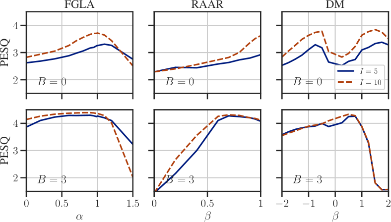
Fig. 3: Mean PESQ score as a function of $\beta$ for different algorithms.

		$B=0$		$B>0$
FGLA		$\alpha=0.99$		$\alpha=0.8$
RAAR		$\beta=0.99$		$\beta=0.7$
DM		$\beta=1.5$		$\beta=0.5$
AGLA		$\alpha_{1}=0.95,\alpha_{2}=0.99,\gamma=1.2$

Table 1: Best performing parameter values with and without look-ahead. Values for FGLA, RAAR, and DM are based on our parameter search (Fig. 3). Values for AGLA are taken from [5].

4 Experimental Evaluation

We evaluate the proposed framework using GLA (equivalent to RTISI) and the other algorithms from Section 2 as underlying algorithms, with various numbers of iterations $I$ and number of look-ahead frames $B$. For FGLA, DM, and RAAR, which have a single tuning parameter, we first perform a parameter search over a plausible range for each algorithm. In the case of AGLA we simply choose the parameter values that are described as best on average in [5]. In all cases we use the same phase initialization scheme as RTISI: after the first $B+1$ frames are initialized with zero-phase, each new frame in $\mathbf{X}_{\text{fluid}}$ is initialized by taking the STFT of the signal estimate up to this point including the phaseless new frame.

4.1 Experimental setting and metrics

All experiments are performed on 100 spoken utterances (gender-balanced) from the TIMIT corpus [28], sampled at 16. All signals are transformed to the STFT domain using a frame length of 32, a frameshift of 8, and a Hann window function. For each utterance $\mathbf{S}$, the magnitude spectrogram $\mathbf{A}=\lvert\mathbf{S}\rvert$ is kept and the phase spectrogram is replaced by zero.

We use the PESQ score (Perceptual Evaluation of Speech Quality) to assess the perceptual quality of reconstructed signals. We also report the spectral convergence (SC), which is a non-perceptual error metric common in phase retrieval studies [29, 14].

4.2 Results

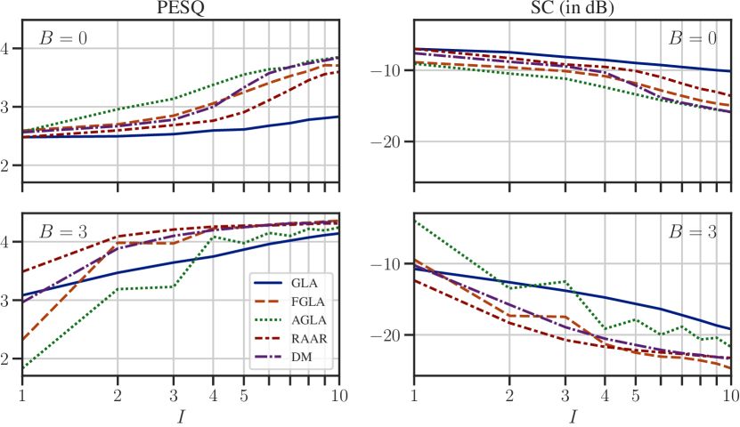
Fig. 4: Mean PESQ and SC as a function of the number of iterations $I$. Except for GLA, each algorithm is evaluated using the parameter values given in Table 1. The horizontal axis is scaled logarithmically.

Results of our parameter search are shown in Fig. 3 in terms of reconstruction quality (mean PESQ) for each algorithm. For brevity, we only show results for $B\in\{0,3\}$, but we note that the behavior for other values of $B>0$ is largely similar to $B=3$. DM shows a comparatively strong sensitivity to the choice of $\beta$, while FGLA delivers good performance across a wide range of $\alpha$, especially for $B>0$. For all three algorithms, the optimal parameter value differs considerably between the look-ahead and non-look-ahead cases. Based on this observation, we use different parameter values for these two cases in the following. The chosen values are listed in Table 1, along with the optimal parameter values for AGLA as determined in [5]. Note that this parameter search is specific to the STFT parameters and type of signals (speech) that we use.

Having found good parameter values, we now analyze the behavior of all algorithms for different numbers of iterations. In Fig. 4 we report results for $I\in\{1,2,\dotsc,10\}$ in terms of PESQ and SC. Compared to GLA (equivalent to RTISI), all algorithms perform considerably better using $I=10$ iterations per frame. This is consistent with results for the offline case [4, 6, 5]. Focusing on the low-iteration regime, we again observe a difference with respect to the number of look-ahead frames $B$. For $B=0$, AGLA consistently performs well, while FGLA, RAAR, and DM only begin to perform considerably better than GLA for $I>3$. However, when including look-ahead frames, RAAR and DM are able to achieve excellent reconstruction quality already with a single iteration, while FGLA and AGLA need a few more iterations to catch up. The same trend has been observed for other values of $B>0$. With parameter tuning, AGLA might perform better for the look-ahead case, but we do not pursue this here. Especially impressive is RAAR’s ability to achieve a PESQ score of about 3.5 with a single iteration per frame and a computational complexity similar to that of GLA.

5 Conclusion

This paper proposes a generalization of the RTISI method for online STFT phase retrieval. By introducing a modified consistency projection and reformulating RTISI in terms of this projection, we are able to show that RTISI, although specifically based on the Griffin-Lim algorithm, can be extended beyond the simple GLA iteration and be used to implement online variants of any iterative projection algorithm in a simple and effective way. The new framework is validated by evaluating on a dataset of speech signals using various underlying algorithms. Evaluation results show that the performance boost offered by improved offline STFT phase retrieval algorithms is also evident in the online case and results in a considerable improvement over RTISI(-LA). The proposed framework will also enable easy online adaptation of novel projection-based algorithms introduced in the future.

6 References

References

- [1] Timo Gerkmann, Martin Krawczyk-Becker and Jonathan Le Roux “Phase Processing for Single-Channel Speech Enhancement: History and Recent Advances” In IEEE Signal Processing Magazine 32.2, 2015, pp. 55–66
- [2] Jonathan Le Roux, Nobutaka Ono and Shigeki Sagayama “Explicit Consistency Constraints for STFT Spectrograms and Their Application to Phase Reconstruction” In Proc. ITRW on Statistical and Perceptual Audio Processing (SAPA 2008), 2008, pp. 23–28
- [3] D. Griffin and Jae Lim “Signal Estimation from Modified Short-Time Fourier Transform” In IEEE Trans. on Audio, Speech, and Lang. Process. (TASLP) 32.2, 1984, pp. 236–243
- [4] Nathanaël Perraudin, Peter Balazs and Peter L. Søndergaard “A Fast Griffin-Lim Algorithm” In IEEE Workshop on Applications of Signal Proc. to Audio and Acoustics (WASPAA), 2013, pp. 1–4
- [5] Rossen Nenov, Dang-Khoa Nguyen and Peter Balazs “Faster Than Fast: Accelerating the Griffin-Lim Algorithm” In IEEE Int. Conf. on Acoustics, Speech and Signal Process. (ICASSP), 2023, pp. 1–5
- [6] Tal Peer, Simon Welker and Timo Gerkmann “Beyond Griffin-Lim: Improved Iterative Phase Retrieval for Speech” In Int. Workshop on Acoustic Signal Enhancement (IWAENC), 2022
- [7] Tomoki Kobayashi, Tomoro Tanaka, Kohei Yatabe and Yasuhiro Oikawa “Acoustic Application of Phase Reconstruction Algorithms in Optics” In IEEE Int. Conf. on Acoustics, Speech and Signal Process. (ICASSP), 2022, pp. 6212–6216
- [8] Jonathan Le Roux, Hirokazu Kameoka, Nobutaka Ono and Shigeki Sagayama “Fast Signal Reconstruction from Magnitude STFT Spectrogram Based on Spectrogram Consistency” In International Conference on Digital Audio Effects (DAFx) 10, 2010, pp. 397–403
- [9] Gerald T. Beauregard, Mithila Harish and Lonce Wyse “Single Pass Spectrogram Inversion” In IEEE International Conference on Digital Signal Processing (DSP), 2015, pp. 427–431
- [10] Yoshiki Masuyama, Kohei Yatabe and Yasuhiro Oikawa “Model-Based Phase Recovery of Spectrograms via Optimization on Riemannian Manifolds” In Int. Workshop on Acoustic Signal Enhancement (IWAENC), 2018, pp. 126–130
- [11] Zdeněk Průša, Peter Balazs and Peter Lempel Søndergaard “A Noniterative Method for Reconstruction of Phase From STFT Magnitude” In IEEE Trans. on Audio, Speech, and Lang. Process. (TASLP) 25.5, 2017, pp. 1154–1164
- [12] Yoshiki Masuyama, Kohei Yatabe and Yasuhiro Oikawa “Griffin–Lim Like Phase Recovery via Alternating Direction Method of Multipliers” In IEEE Signal Process. Lett. (SPL) 26.1, 2019, pp. 184–188
- [13] Shinnosuke Takamichi, Yuki Saito, Norihiro Takamune, Daichi Kitamura and Hiroshi Saruwatari “Phase Reconstruction from Amplitude Spectrograms Based on Von-Mises-Distribution Deep Neural Network” In Int. Workshop on Acoustic Signal Enhancement (IWAENC), 2018, pp. 286–290
- [14] Yoshiki Masuyama, Kohei Yatabe, Yuma Koizumi, Yasuhiro Oikawa and Noboru Harada “Deep Griffin–Lim Iteration: Trainable Iterative Phase Reconstruction Using Neural Network” In IEEE J. Sel. Top. Signal Process. (JSTSP) 15.1, 2021, pp. 37–50
- [15] Nguyen Binh Thien, Yukoh Wakabayashi, Kenta Iwai and Takanobu Nishiura “Inter-Frequency Phase Difference for Phase Reconstruction Using Deep Neural Networks and Maximum Likelihood” In IEEE Trans. on Audio, Speech, and Lang. Process. (TASLP) 31, 2023, pp. 1667–1680
- [16] Tal Peer, Simon Welker and Timo Gerkmann “DiffPhase: Generative Diffusion-Based STFT Phase Retrieval” In IEEE Int. Conf. on Acoustics, Speech and Signal Process. (ICASSP), 2023, pp. 1–5
- [17] Gerald T Beauregard, Xinglei Zhu and Lonce Wyse “An Efficient Algorithm for Real-Time Spectrogram Inversion” In International Conference on Digital Audio Effects (DAFx), 2005, pp. 116–118
- [18] Xinglei Zhu, Gerald T. Beauregard and Lonce Wyse “Real-Time Iterative Spectrum Inversion with Look-Ahead” In IEEE Int. Conf. on Multimedia and Expo, 2006, pp. 229–232
- [19] Xinglei Zhu, Gerald T. Beauregard and Lonce L. Wyse “Real-Time Signal Estimation From Modified Short-Time Fourier Transform Magnitude Spectra” In IEEE Trans. on Audio, Speech, and Lang. Process. (TASLP) 15.5, 2007, pp. 1645–1653
- [20] Volker Gnann and Martin Spiertz “Improving RTISI Phase Estimation with Energy Order and Phase Unwrapping” In International Conference on Digital Audio Effects (DAFx) 10, 2010
- [21] Jonathan Le Roux, Hirokazu Kameoka, Nobutaka Ono and Shigeki Sagayama “Phase Initialization Schemes for Faster Spectrogram-Consistency-Based Signal Reconstruction” In Proceedings of the Acoustical Society of Japan Autumn Meeting 3, 2010
- [22] Zdeněk Průša and Pavel Rajmic “Toward High-Quality Real-Time Signal Reconstruction From STFT Magnitude” In IEEE Signal Process. Lett. (SPL) 24.6, 2017, pp. 892–896
- [23] Zdeněk Průša and Peter L Søndergaard “Real-Time Spectrogram Inversion Using Phase Gradient Heap Integration” In International Conference on Digital Audio Effects (DAFx), 2016, pp. 17–21
- [24] Yoshiki Masuyama, Kohei Yatabe, Kento Nagatomo and Yasuhiro Oikawa “Online Phase Reconstruction via DNN-Based Phase Differences Estimation” In IEEE Trans. on Audio, Speech, and Lang. Process. (TASLP) 31, 2023, pp. 163–176
- [25] Nguyen Binh Thien, Yukoh Wakabayashi, Yuting Geng, Kenta Iwai and Takanobu Nishiura “Weighted Von Mises Distribution-based Loss Function for Real-time STFT Phase Reconstruction Using DNN” In ISCA Interspeech ISCA, 2023, pp. 3864–3868
- [26] D. Luke “Relaxed Averaged Alternating Reflections for Diffraction Imaging” In Inverse Problems 21.1 IOP Publishing, 2004, pp. 37–50
- [27] Veit Elser “Phase Retrieval by Iterated Projections” In Journal of the Optical Society of America A 20.1, 2003, pp. 40
- [28] J.. Garofolo, L.. Lamel, W.. Fisher, J.. Fiscus, D.. Pallett and N.. Dahlgren “DARPA TIMIT Acoustic Phonetic Continuous Speech Corpus CDROM” Gaithersburg, MD, USA: National Institute of Standards and Technology (NIST), 1993
- [29] Nicolas Sturmel and Laurent Daudet “Signal Reconstruction from STFT Magnitude: A State of the Art” In International Conference on Digital Audio Effects (DAFx), 2011, pp. 375–386