A linear model of synergetic current drive with lower-hybrid wave and electron cyclotron wave

Abstract

A linear model of synergetic current drive (SCD) with lower-hybrid wave (LHW) and electron cyclotron wave (ECW) is proposed to efficiently calculate the quantitative SCD efficiency and reveal the conditions for the occurrence of SCD. In this model, the response function dominated by collisions in the presence of LHW is derived from the adjoint equations by using perturbation and Green-Function techniques, where the relativistic effect and the trapped effect are taken into account. The SCD efficiency is compared with the commonly used ECW current drive (ECCD) efficiency in the parameter space using our linear model. The results show two features of the synergy effect, One is that it is inclined to occurs at smaller $y=2\omega_{c}/\omega$ with the fixed ECW parallel refractive index $n_{\parallel}$, and the other is that the threshold values of $y$, at which the synergy effect becomes sufficiently significant, shifts towards higher values with a decreasing $n_{\parallel}$. The quasilinear simulation on ECCD and SCD efficiency with a two-dimensional Fokker-Planck code are consistent with the results of the linear model in trends. Based on the linear SCD efficiency, criteria for the occurrence and the sufficient significance of the synergy effect are suggested, which indicate that the synergy effect is dependent on the power factor that quantifies the degree of the overlap of the two waves’ quasilinear domains, the LHW power, and synergy electrons. The present work provides a method of quick matching and calculating of SCD with LHW and ECW, and may be important for the real-time application of the SCD in future reactors.

• November 2023

Keywords: current drive, the synergy effect, lower-hybrid wave, electron cyclotron wave.

1 Introduction

In Tokamak, the use of ratio frequency waves (RF) injection for current drive (CD)[1] to realize active control of plasma current profile can not only suppress turbulent transport and stabilize MHD but also is crucial to achieve long-pulse steady-state operation in the future reactor. The principle of RF CD is to use an external device to inject asymmetric momentum into plasmas or establish asymmetric resistivity in plasmas. The typical applications for experiments corresponding to different mechanisms respectively are lower-hybrid wave current drive (LHCD) and electron cyclotron wave current drive (ECCD). Both of them transfer the energy of the wave to resonant particles, then a net particle flow(i.e. current) is driven. LHCD has high CD efficiency but its current profile is not easy to control, and ECCD has high locality and positive maneuverability but CD efficiency is small. Based on their complementary properties, the idea of synergetic current drive(SCD) has been proposed[2] for optimizing the driven current. Subsequently, both the simulation using a three-dimensional Fokker-Planck code[3] and the model combining kinetic process[7] manifest the main feature of SCD is that the current driven by lower-hybrid waves (LHW) and electron cyclotron waves (ECW) simultaneously $I_{LH+EC}$ can be larger than the sum of currents driven individually $I_{LH}+I_{EC}$ in the same plasma conditions, and this phenomenon is called the synergy effect. SCD was firstly achieved in stationary conditions on the Tore Supra[4], the core experimental phenomenon is the improvement(up to a factor of $\sim 4$) of ECCD efficiency sustained by LHCD, and the synergy effect is demonstrated experimentally.

Numerical simulations provide further valuable insights into SCD, despite their time-consuming nature. The synergy effect is influenced by the radial location $\rho_{EC}$ of maximum ECW power deposition[4] and the resonance relationship between LHW and ECW in velocity space[8]. When there is an overlap of power deposition of LHW and ECW in radial location, as well as an overlap of the quasilinear domains in velocity space, the synergy effect occurs. The dependence of this effect on the frequency $\omega$ and parallel refractive index $n_{\parallel}$ of resonance curve of ECW has been investigated[21]. Additionally, other kinetic simulations have shown a negative effect[14] when the ECW power greatly exceeds the LHW power, and a new synergy mechanism[15] between ECCD based on the Ohkawa effect and LHCD has been observed even in the absence of overlapping quasilinear domains.

The understanding of the synergy effect remains qualitative although simulations have revealed various properties of SCD. The pioneering work[8] from the theoretical analysis has qualitatively proved the existence of the synergy effect by using perturbation technique, but there is less work investigating SCD quantitatively. However, ECCD[9, 10] and LHCD[1, 11] both have been investigated quantitatively from a theoretical perspective and integrated into ray-tracing codes such as TORAY-GA[12] and GENRAY[13], which benefit fusion plasma simulation a lot. Therefore, developing a linear model of SCD can not only rapidly calculate SCD efficiency quantitatively and deepen the understanding of the synergy effect, but also have enormous application potential that integrates the linear model into ray-tracing codes profiting for real-time control of plasma confinement. For the aim to establish it in this paper, the adjoint method [16, 1], the techniques of perturbation[8] and Green-Function[10, 8], and Legendre expansion[10] in pitch-angle $\xi=v_{\parallel}/v$ have been applied to solve the response function in the presence of LHW at low-collisionality regime[17] and calculate SCD efficiency. The relativistic effect and the trapped effect are taken into account in calculations. The magnetic well is approximated as a square well for convenience, and the results of SCD are benchmarked against those of ECCD[10].

The organization of the paper is as follows. Section 2 focuses on establishing the linear model. Section 3 presents the criteria for measuring the synergy effect. Finally, a summary is in the Section 4. Appendix A presents the details of the zero-order response function $\tilde{\chi}_{0}$. In Appendix B, we evaluate the effectiveness of approximation that takes $F(u)$ as a simple function with fixed order and coefficient in numerical calculation. Appendix C presents the interpolation formula for the angular part of the perturbation response function.

2 The linear model of SCD

The motion of electrons is characterized by the relativistic dynamics in following derivation. Let $\mathbf{u}=\mathbf{p}/m=\gamma\mathbf{v}$ with $\gamma=\sqrt{1+(u/c)^{2}}$ denotes the momentum per unit mass and the kinetic particle energy is $w=(\gamma-1)mc^{2}$. On the premise of low RF power density, the electron distribution function in the presence of RF satisfies

$$f=f_{M}+\delta f,$$ (1)

where $f_{M}$ is the Maxwellian distribution, $\delta f$ is the perturbed distribution function caused by external energy injection, both are considered as a function of kinetic energy $w$, magnetic moment $\mu=mu_{\perp}^{2}/2B$, and poloidal angle of a given flux surface $\theta_{p}$. The premise also implies the interaction between waves and electrons can be portrayed by $S_{rf}(f_{M})$. Ignoring the small cross-effect drifts and finite banana width, the linearized Fokker-Planck equation, which describes the dynamic behavior of perturbed distribution $\delta f$, can be written as

$$v_{\parallel}\mathbf{\hat{b}}\cdot\nabla\delta f-\hat{O}\delta f=S_{\mathrm{rf}}\left(f_{M}\right),$$ (2)

where $\hat{O}$ denotes a linearized operator. The response function $\chi$ associated with driven current caused by the perturbed function statisfies

$$-v_{\parallel}\hat{\mathbf{b}}\cdot\nabla\chi-\hat{O}^{\dagger}\chi=\frac{v_{\parallel}B}{\left\langle B^{2}\right\rangle},$$ (3)

where $\hat{O}^{\dagger}$ is the adjoint operator of $\hat{O}$:

$$\int d\mathbf{u}(\hat{O}^{\dagger}h(\mathbf{u}))g(\mathbf{u})=\int d\mathbf{u}h(\mathbf{u})\hat{O}g(\mathbf{u}).$$ (4)

Following Lin-Liu[10], the CD efficiency and the dimensionless CD efficiency used by experimentists [22] are

$$\zeta^{*}=\frac{e^{3}}{\varepsilon_{0}^{2}}\frac{n_{e}}{T_{e}}\frac{\left\langle j_{\parallel}\right\rangle}{2\pi Q}=-\frac{4}{\ln\Lambda}\left\langle\frac{B}{B_{m}}\right\rangle\frac{\left\langle\int d\Gamma\tilde{\chi}S_{\mathrm{rf}}\left(f_{M}\right)\right\rangle}{\left\langle\int d\Gamma\left(w/mv_{e}^{2}\right)S_{\mathrm{rf}}\left(f_{M}\right)\right\rangle},$$ (5)

$$\tilde{\zeta}=\frac{e^{3}}{\varepsilon_{0}^{2}}\frac{n_{e}}{T_{e}}\frac{R_{p}I}{P}=\frac{R_{p}}{\langle B\rangle}\langle\frac{B_{\phi}}{R}\rangle\zeta^{*}.$$ (6)

with

$$\left\langle j_{\parallel}\right\rangle=-e\langle\int d\Gamma\delta fv_{\parallel}\rangle=-e\langle B\int d\Gamma\chi S_{\mathrm{rf}}\left(f_{M}\right)\rangle,$$ (7)

$$Q=\left\langle\int d\Gamma wS_{\mathrm{rf}}\left(f_{M}\right)\right\rangle,$$ (8)

$$\langle\cdots\rangle=\frac{\oint\frac{d\ell_{p}}{B_{p}}\ldots}{\oint\frac{d\ell_{p}}{B_{p}}},$$ (9)

$$\tilde{\chi}=\nu_{e0}\left(B_{m}/v_{e}\right)\chi.$$ (10)

Here $\varepsilon_{0}$ is the permittivity of free space, $\langle j_{\parallel}\rangle$ is the wave-driven current, $Q$ is the absorbed wave power density, $B_{m}$ is the maximum of $B$ at the flux surface, $d\Gamma$ is the volume element in velocity space, $\langle...\rangle$ represents the flux-surface average, $dl_{p}$ is the line element along the poloidal circumference, $B_{p}$ is the poloidal magnetic field, $\tilde{\chi}$ is the dimentionless response function of $\chi$. $n_{e}$, $T_{e}$, $v_{e}=\sqrt{2T_{e}/m}$, $\ln\Lambda$, and $\nu_{e0}=(e^{4}n_{e}ln\Lambda)/(4\pi\epsilon_{0}^{2}m^{2}v_{e}^{3})$ are electron density, electron temperature, electron thermal velocity, Coulomb logarithm, and collision frequency, respectively.

The theoretical formulation of RF CD in above derivations is universal as long as the wave injection does not significantly make the electron distribution deviating from the Maxwellian distribution, which is consistent with the premise of low RF power density. In ECCD case[10], $\hat{O}$ and $S_{rf}(f_{M})$ are replaced by the linearized collision operator $\hat{C}$ and the operator indicating interaction between ECW and electrons. Here $\hat{C}$ in the Fisch’s relativistic high-velocity model[1] can be writen as

$$\hat{C}f=\left[\nu_{ei}(u)+\nu_{D}(u)\right]Lf+\frac{1}{u^{2}}\frac{\partial}{\partial u}u^{2}\lambda_{s}(u)f,$$ (11)

where L denotes the pitch-angle scattering operator

$$L=\frac{1}{2}\frac{\partial}{\partial\xi}\left(1-\xi^{2}\right)\frac{\partial}{\partial\xi},$$ (12)

with $\xi=\frac{v_{\parallel}}{v}$, and the pitch-angle scattering rates because of electron-ion and electron-electron collisions are

$$\nu_{ei}(u)=Z_{\mathrm{eff}}\nu_{e0}\gamma\left(\frac{u_{e}}{u}\right)^{3},$$ (13)

$$\nu_{D}(u)=\nu_{e0}\gamma\left(\frac{u_{e}}{u}\right)^{3},$$ (14)

in which $Z_{eff}$ is the effective charge and $u_{e}=v_{e}=\sqrt{2T_{e}/m}$. The last term of Eq.(11) describes the slowing-down effect because of electron-electron collisions and the rate is

$$\lambda_{s}(u)=\nu_{e0}u_{e}\gamma^{2}\left(\frac{u_{e}}{u}\right)^{2}.$$ (15)

Additionally, the adjoint operator of $\hat{C}$ is

$$\hat{C}^{\dagger}g=\left[\nu_{ei}(u)+\nu_{D}(u)\right]Lg-\lambda_{s}(u)\frac{\partial}{\partial u}g.$$ (16)

Based on the experimental phenomenon of the synergy effect, the improvement of ECCD efficiency in the presence of LHW, following R.Dumont[8], we consider the electron relaxation is dominant by collisions and diffusions caused by the LHW power in a given velocity space together, where collisions are the leading role, such that operator $\hat{O}$ will be regarded as $\hat{C}+\hat{D_{LH}}$, and $S_{rf}(f_{M})$ is the same with ECCD case which describes the interaction between ECW and electrons. It implies that ECW will act on the electrons distribution altered by the injection of the LHW power $f=f_{M}(1+\phi)$, in which $f_{M}\phi$ represents the modification caused by LHW effect and is also a perturbation quantity, so that the SCD efficiency calculated in this situation by using $S_{rf}({f_{M}})$ is still effective. Here $\hat{D_{LH}}$ is a linearized operator describing diffusions induced by LHW power in a given parallel velocity space since the main mechanism of LHCD is Landau damping, which can be written as

$$\hat{D}_{\mathrm{LH}}\equiv\nu_{e0}u_{e}^{2}\frac{\partial}{\partial u_{\parallel}}D_{\mathrm{LH}}\left(u_{\parallel}\right)\frac{\partial}{\partial u_{\parallel}},$$ (17)

with

$$D_{LH}\left(u_{\parallel}\right)\equiv\left\{\begin{array}[]{ll}0,u_{\parallel}<u_{\parallel,1}\\ Const.,\quad u_{\parallel,1}\leq u_{\parallel}\leq u_{\parallel,2}\\ 0,u_{\parallel}>u_{\parallel,2}\end{array}\right.$$ (18)

where $D_{LH}$ is a constant determined by the wave power[7]. In addition, $\hat{D}_{LH}$ is a self-adjoint operator (i.e., $\hat{D}_{LH}^{\dagger}=\hat{D}_{LH}$).

Combined the two operator $\hat{C^{\dagger}}$ and $\hat{D}_{LH}^{\dagger}$, the Eq.(3) can be rewritten as

$$-v_{\parallel}\hat{b}\cdot\nabla\chi-\hat{C}^{\dagger}\chi-\hat{D}_{LH}^{\dagger}\chi=\frac{v_{\parallel}B}{\left\langle B^{2}\right\rangle}.$$ (19)

The problem of solving SCD efficiency is reduced to obtain the analytical form of dimensionless response function $\tilde{\chi}$ corresponding to $\chi$ through Eq.(19), and then compute the integral Eq.(5) with given $S_{ECW}(f_{M})$. The following subsections will be arranged to acquire dimensionless response function $\tilde{\chi}$ by using perturbation and Green-Function techniques and to calculate the SCD efficiency versus the ECCD only case , then we use a two-dimensional Fokker-Planck code to examine the accuracy of linear model through quasilinear simulations.

2.1 The response function

The assumption in ECCD[10] that the effective collisional frequency is much smaller than the bounced frequency , i.e., $(\nu_{e0}/\epsilon)/\omega_{b}\ll 1$ where $\epsilon$ is the inverse aspect ratio, is also adopted in ours, such that the trapped electrons are allowed to complete the banana orbits at all energies. Therefore, the response function $\chi$ has an expansion in this parameter (i.e., $\chi=\chi_{I}+\chi_{II}+...$), for passing electrons Eq.(19) can be writen as

$$\frac{1}{v}\left\langle\frac{B}{|\xi|}(C^{\dagger}+D_{LH}^{\dagger})\right\rangle\chi_{I}=-sgn(v_{\parallel}).$$ (20)

The subscript $I$ of $\chi_{I}$ will be omitted in following derivations for articulating due to the limitation of banana regime.

According to the previous assumption that collisions still dominate the process of electron relaxation although the diffusions caused by LHW affect electrons dynamic behavior in a given parallel velocity space, we can linearize $\chi$

$$\chi={\chi}_{0}+{\delta\chi},$$ (21)

in which $D_{LH}$ is the small parameter. Substituting Eq.(21) into Eq.(20), by using perturbation technique, we obtain the zero-order equation

$$\frac{1}{v}\left\langle\frac{B}{|\xi|}C^{\dagger}\right\rangle\chi_{0}=-sgn(v_{\parallel}),$$ (22)

and the first-order equation

$$\langle\frac{B}{|\xi|}C^{\dagger}\rangle{\delta\chi}=-\langle\frac{B}{|\xi|}D_{LH}^{\dagger}\rangle{\chi}_{0}.$$ (23)

Lin-Liu[10] has given a useful solution for dimensionless response function $\tilde{\chi}_{0}$ corresponding to $\chi_{0}$ by separating variables $u,\lambda$ and using Green-Function technique

$$\tilde{\chi}_{0}=sgn(u_{\parallel})F(u)H(\lambda),$$ (24)

where $\lambda=\frac{\mu B_{m}}{mu^{2}/2}=\frac{B_{m}}{B}\frac{u_{\perp}^{2}}{u^{2}}$ is a new pitch-angle variable. For passing electrons, $\lambda$ is in range of $0\leq\lambda<1$, and for trapped particles $1\leq\lambda<\frac{B_{m}}{B}$, at a given poloidal angle. The more details of Eq.(24) are in Appendix A.

Now the specific form of first-order equation associating with dimensionless response function is

$$(\nu_{ei}+\nu_{D})\bar{L}\tilde{\delta\chi}-\lambda_{s}(u)\langle\frac{B}{B_{m}}\frac{1}{|\xi|}\frac{\partial}{\partial u}\tilde{\delta\chi}\rangle=-\nu_{e0}u_{e}^{2}\langle\frac{B}{B_{m}}\frac{1}{|\xi|}\frac{\partial}{\partial u_{\parallel}}D_{LH}\frac{\partial}{\partial u_{\parallel}}\tilde{\chi}_{0}\rangle,$$ (25)

where $\bar{L}$ is the bounce averaged pitch-angle scattering operator

$$\bar{L}=\langle\frac{B}{B_{m}}\frac{1}{|\xi|}L\rangle=2\frac{\partial}{\partial\lambda}\lambda\langle|\xi|\rangle\frac{\partial}{\partial\lambda}.$$ (26)

In order to obtain the analytical form of $\tilde{\delta\chi}$, firstly we approximate the zero-order response function $\tilde{\chi}_{0}$ in the right side of Eq.(26) by keeping the first term of its Legendre expansion in $\xi$

$$\langle\frac{B}{B_{m}}\tilde{\chi}_{0}\rangle \simeq\langle\frac{B}{B_{m}}p_{1}(\xi)\frac{3}{2}\int_{-1}^{1}d\xi\tilde{\chi}_{0}(u,\xi,\theta_{p})p_{1}(\xi)\rangle$$ (27)

$$=\langle p_{1}(\xi)\rangle\frac{3}{2}\langle\frac{B^{2}}{B_{m}^{2}}\rangle\int_{0}^{\frac{B_{m}}{B}}d\lambda sgn(u_{\parallel})\tilde{\chi}_{0}(u,\lambda)$$ (28)

$$=f_{c}F(u)\langle\xi\rangle,$$ (29)

with the fact $p_{1}(\xi)=\xi$ and $f_{c}$ is the effective circulating particle fraction in the neoclassical transport theory[19, 10]. Substituting it into the right-hand side of Eq.(25) and using

$$\frac{\partial}{\partial u_{\parallel}}=\xi\frac{\partial}{\partial u}+\frac{1}{u}(1-\xi^{2})\frac{\partial}{\partial\xi},$$ (30)

we have

$$\nu_{e0}u_{e}^{2}\langle\frac{1}{|\xi|}\frac{\partial}{\partial u_{\parallel}}D_{LH}\frac{\partial}{\partial u_{\parallel}}(f_{c}F(u)\xi)\rangle$$ (31)

$$=sgn(u_{\parallel})\nu_{e0}u_{e}^{2}f_{c}D_{LH}\bigg{\langle}\left[\xi^{2}\frac{\partial^{2}}{\partial u^{2}}F(u)+\frac{3(1-\xi^{2})}{u}\frac{\partial F(u)}{\partial u}+\frac{-3(1-\xi^{2})}{u^{2}}F(u)\right]\bigg{\rangle}.$$ (32)

For the convenience of calculation, we approximate $F(u)$ as a simple function with fixed order in numerically

$$F(u)=C_{k}(\frac{u}{u_{e}})^{k},$$ (33)

here $C_{k}$ is a coefficient and $k$ is the fixed order. The specific form of $F(u)$ and its derivatives we adopted in following derivations and discussions on their effectiveness are in appendix B. Substituting Eq.(30) into Eq.(29), then Eq.(25) reduces to

$$(\nu_{ei}+\nu_{D})\bar{L}\tilde{\delta\chi}-\lambda_{s}(u)\langle\frac{B}{B_{m}}\frac{1}{|\xi|}\rangle\frac{\partial}{\partial u}\tilde{\delta\chi}=-sgn(u_{\parallel})D_{LH}A_{1}\frac{u^{k-2}}{u_{e}^{k-2}}D_{k}(\lambda),$$ (34)

where

$$D_{k}(\lambda)=\langle\left[(k-3)\xi^{2}+3\right]\rangle=(3-k)\lambda h_{1}+k,$$ (35)

with $A_{1}=(k-1)C_{k}f_{c}$ and $h_{1}=\langle\frac{B}{B_{m}}\rangle$. We suppose the perturbation response function still can be separated by variables $u,\lambda$, which results in a useful form

$$\frac{\tilde{\delta\chi}}{D_{k}(\lambda)}=\tilde{\delta\chi}^{\prime}=sgn(u_{\parallel})S(u)M(\lambda).$$ (36)

Likely, we adopt the same technique to approximate the slowing-down part of Eq.(31)

$$\lambda_{s}(u)\langle\frac{B}{B_{m}}\frac{1}{|\xi|}\frac{\partial}{\partial u}\tilde{\delta\chi}^{\prime}\rangle \simeq sgn(u_{\parallel})\lambda_{s}(u)\frac{3}{2}\langle\frac{B^{2}}{B_{m}^{2}}\rangle\int_{0}^{1}d\lambda M(\lambda)\frac{\partial S(u)}{\partial u}$$ (37)

$$=sgn(u_{\parallel})f_{n}\lambda_{s}(u)\frac{\partial S(u)}{\partial u},$$ (38)

where

$$f_{n}=\frac{3}{2}\langle\frac{B^{2}}{B_{m}^{2}}\rangle\int_{0}^{1}d\lambda M(\lambda),$$ (39)

in which trapped particles are not included in the integral. Thus the first-order equation becomes

$$\frac{1}{D_{k}(\lambda)}(\nu_{ei}+\nu_{D})S(u)\bar{L}D_{k}(\lambda)M(\lambda)-\lambda_{s}(u)f_{n}\frac{\partial}{\partial u}S(u)=-D_{LH}A_{1}\frac{u^{k-2}}{u_{e}^{k-2}}.$$ (40)

Furthermore, we take the equation about $\lambda$ satisfying

$$\bar{L}D_{k}(\lambda)M(\lambda)=-D_{k}(\lambda),$$ (41)

for $0<\lambda<1$. With the regular boundary condition at $\lambda=0$ and a new definition $E_{k}(\lambda)\equiv D_{k}(\lambda)M(\lambda)$, we obtain

$$E_{k}(\lambda)=\frac{\theta(1-\lambda)}{2}\int_{\lambda}^{1}d\lambda^{\prime}\frac{D_{k}(\lambda^{\prime})}{\langle(1-\lambda^{\prime}B/B_{m})^{1/2}\rangle},$$ (42)

the more useful forms about $E(\lambda)$ are in appendix C.

For now we are able to separate the equation about $u$

$$(\nu_{ei}+\nu_{D})S(u)+\lambda_{s}(u)f_{n}\frac{\partial}{\partial u}S(u)=D_{LH}A_{1}\frac{u^{k-2}}{u_{e}^{k-2}}.$$ (43)

Substituting coefficients and using Green-Function technique, where the green function is

$$G(u,u^{\prime})=\theta(u-u^{\prime})(\frac{u^{\prime}}{u})^{\rho^{\prime}}(\frac{\gamma+1}{\gamma^{\prime}+1})^{\rho^{\prime}},$$ (44)

with the boudary condition $S(0)=0$, we find the relativistic form of $S(u)$

$$S_{r}(u) =D_{LH}A_{2}\frac{1}{u_{e}}(\frac{\gamma+1}{u})^{\rho^{\prime}}\int_{0}^{u}du^{\prime}(\frac{u^{\prime}}{\gamma^{\prime}+1})^{\rho^{\prime}}(\frac{u^{\prime}}{u_{e}})^{k}(\frac{1}{\gamma^{\prime}})^{2}$$ (45)

$$=D_{LH}A_{2}(\gamma+1)^{\rho^{\prime}}(\frac{u}{u_{e}})^{k+1}\int_{0}^{1}dyy^{\rho^{\prime}+k}\frac{1}{(\gamma^{\prime}_{y}+1)^{\rho^{\prime}}}\frac{1}{(\gamma^{\prime}_{y})^{2}},\quad$$ (46)

where $\rho^{\prime}=\frac{Z_{eff}+1}{f_{n}}$, $\gamma^{\prime}_{y}=\sqrt{1+(uy/c)^{2}}$, and $A_{2}=\frac{A_{1}}{f_{n}}=(k-1)C_{k}\frac{f_{c}}{f_{n}}$.

To sum up, we have the semi-analytical relativistic response function $\tilde{\delta\chi}$ to describe the perturbation of electron relaxation caused by LHW effect in a given parallel velocity space

$$\tilde{\delta\chi}=sgn(u_{\parallel})S(u)E(\lambda).$$ (47)

Although diffusions induced by LHW power is able to influence electron’s behavior outside of a given region through pitch-angle scattering revealed by kinetic simulation, this effect will exponentially decay so that we can esteem $\tilde{\delta\chi}$ only appear in the given region, which is consistent with the fact that $D_{LH}$ equals zero outside of a given region. In addition, by letting $c\to\infty$ and using the non-relativistic form of $F(u)$[10, 20] with $k=4$ and $C_{k}=1/(Z_{eff}+1+4f_{c})$, we have the non-relativistic form of $S(u)$

$$S_{nr}(u) =D_{LH}(k-1)\frac{C_{k}}{Z_{eff}+1+kf_{n}}\frac{f_{c}}{f_{n}}(\frac{u}{u_{e}})^{k+1}$$ (48)

$$=3D_{LH}\frac{1}{(Z_{eff}+1+4f_{c})(Z_{eff}+1+4f_{n})}\frac{f_{c}}{f_{n}}(\frac{u}{u_{e}})^{5}.$$ (49)

2.2 The SCD efficiency

According to previous discussions, we need $S_{rf}(f_{M})$ characterizing properties of ECW to calculate the SCD efficiency, i.e., the ECCD efficiency in the presence of LHW. Following Cohen[9], the simplified quasilinear diffusion operator for ECW is

$$S_{ECW}(f)=\delta(x-x_{R})\tilde{\Lambda}D_{ECW}\delta(\omega-k_{\parallel}v_{\parallel}-\ell\frac{\omega_{c}}{\gamma})\tilde{\Lambda}f,$$ (50)

with $\tilde{\Lambda}=\frac{\partial}{\partial w}+\frac{k_{\parallel}}{\omega}\frac{\partial}{\partial p_{\parallel}}$. Here, $x_{R}$ denotes the spatial location of ECW power deposition, $D_{ECW}$ is the quasilinear diffusion coefficient, $\omega,\omega_{c},k_{\parallel},\ell$, respectively, are the frequency of ECW, the local cylotron frequency, the parallel wave number of ECW and the harmonic number. According to the previous assumption about power deposition, and then following Lin-Liu[10], the SCD efficiency can be written as

$$\zeta^{*}_{SCD}=-\frac{4}{\ln\Lambda}\left\langle\frac{B}{B_{m}}\right\rangle\frac{mu_{e}^{2}\int d\gamma\left(u_{\perp}\right)^{2\ell}f_{M}\tilde{\Lambda}\tilde{\chi}}{\int d\gamma\left(u_{\perp}\right)^{2\ell}f_{M}},$$ (51)

where $u_{\perp}^{2}=c^{2}\left[\gamma^{2}-1-(\frac{\gamma-y}{n_{\parallel}})^{2}\right]$, $n_{\parallel}=k_{\parallel}c/\omega$ and $y=\ell\omega_{c}/\omega$. The upper $\gamma_{max}$ and lower $\gamma_{min}$ bounds of integrals are determined by

$$\gamma^{2}-1-(\frac{\gamma-y}{n_{\parallel}})^{2}=0.$$ (52)

Using the linearized response function, we have

$$mu_{e}^{2}\tilde{\Lambda}\tilde{\chi}=mu_{e}^{2}\tilde{\Lambda}(\tilde{\chi}_{0}+\tilde{\delta\chi}),$$ (53)

with

$$mu_{e}^{2}\widetilde{\Lambda}\widetilde{\delta\chi}=\gamma\frac{u_{e}^{2}}{u}\frac{\partial}{\partial u}\widetilde{\delta\chi}+2\frac{B_{\max}}{B}\frac{u_{\|}u_{e}^{2}}{u^{3}}\left(\frac{\gamma u_{\|}}{u}-\frac{n_{\|}u}{c}\right)\frac{\partial}{\partial\lambda}\widetilde{\delta\chi}$$ (54)

$$=sgn\left(u_{\|}\right)\left\{\gamma\frac{u_{e}^{2}}{u}\frac{dS}{du}E+2\frac{B_{\max}}{B}\frac{u_{\|}u_{e}^{2}}{u^{3}}\right.\left.\times\left(\frac{\gamma u_{\|}}{u}-\frac{n_{\|}u}{c}\right)S\frac{dE}{d\lambda}\right\}.$$ (55)

Thus the Eq.(47) actually implies

$$\zeta^{*}_{SCD}=\zeta^{*}_{ECCD}+\zeta^{*}_{syn}.$$ (56)

The term in Eq.(47) $mu_{e}^{2}\tilde{\Lambda}\tilde{\chi}_{0}$ and $\zeta_{ECCD}^{*}$ both have been given by Lin-Liu[10]. The $\zeta^{*}_{SCD}$ is a function of electron temperature $T_{e}$, parallel refractive index $n_{\parallel}$, effective charge $Z_{eff}$, the parameter $y=\ell\omega_{c}/\omega$, the inverse aspect ratio $\varepsilon$, the poloidal angle $\theta_{p}$, the constant $D_{LH}$ determined by the LHW power, and the given parallel velocity boundaries $u_{\parallel,1}$ and $u_{\parallel,2}$.

2.3 Theoretical results of SCD efficiency

For now we can calculate the $\tilde{\zeta}_{SCD}(Te,n_{\parallel},Z_{eff},y,\varepsilon,\theta_{p},D_{LH},u_{\parallel,1},u_{\parallel,2})$ though Eq.(6, 24, 38, 41, 45-49). In order to benchmark SCD’s results with ECCD’s, we take the same plasma and magnetic field parameters as the ECCD case[10], these and LHW parameters are shown in Tab.1. We depict the dimensionless SCD efficiency as a function of $y=\frac{2\omega_{c}}{\omega}$ with different polodial angle $\theta_{p}$, the results are shown in Fig.1.

Table 1: Plasma, magnetic field and LHW parameters

$T_{e}$	2000
$n_{\parallel}$	0.3, 0.5, 0.7
$Z_{eff}$	1.6
Inverse Aspect Radio	0.2
$\theta_{p}$	$\frac{\pi}{12},\frac{\pi}{2},\frac{11\pi}{12}$
$n_{e}$	$2*10^{19}$
torodial field	$B=B_{0}/(1+\varepsilon cos\theta_{p})$
polodial field	$B=B_{p0}/(1+\varepsilon cos\theta_{p})$
R	1.76m
$D_{LH}$	10
$u_{\parallel,1}$	$3u_{e}$
$u_{\parallel,2}$	$5u_{e}$

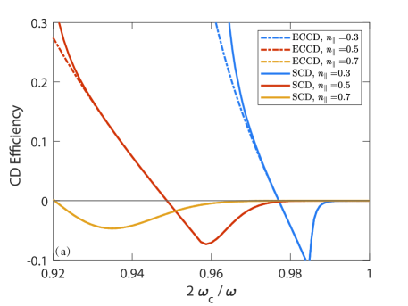
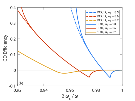
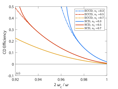
Figure 1: The ECCD(dashed lines) and SCD(solid lines) efficiency at different poloidal angles (a)$\theta_{p}=15^{\circ}$(weak-field side), (b) $\theta_{p}=90^{\circ}$ and (c)$\theta_{p}=165^{\circ}$ at a given flux surface. The color of line denotes different parallel refractive index of ECW.

The three panels indicate the existence of the improvement of ECCD efficiency in the presence of LHW (i.e., the synergy effect) in certain parameters space. Comparing the results of ECCD and SCD, the line trends reveal the two features. One is that the threshold values of $y$, at which the synergy effect becomes sufficiently significant, shifts towards higher values with a decreasing $n_{\parallel}$. The other important feature is that the synergy effect is inclined to occur in smaller y with fixed $n_{\parallel}$, which is consistent with the previous understanding of SCD’s mechanism based on the kinetic simulation: the overlap of quasilinear domains of ECW and LHW. The reflection of the overlap in velocity space is the matching pattern between the resonance curve of ECW and the diffusion region of LHW. Thus we select a typical case of the above situations with $\theta_{p}=90^{\circ}$ and $n_{\parallel}=0.5$ to explain the feature, as shown in Fig.2.

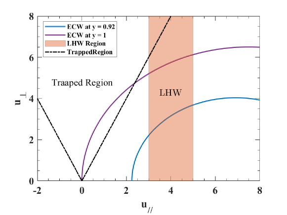
Figure 2: Resonance curves of ECW(the blue line: $y=0.92$, the purple line: $y=1$), the diffusion region of LHW (the orange area), and the trapped region (the area within the two black dashed lines) in velocity space.

Varying from $y=0.92$ to $y=1$, the resonance curve of ECW changes from the blue line to the purple line. The diffusion region of LHW is fixed with $u_{\parallel,1}=3$ and $u_{\parallel,2}=5$ (normalized to the thermal velocity). The area within the two black lines is the trapped region. For ECCD only, the efficiency changes from positive to negative as increasing $y$ because the low-energy part of resonance curve of ECW (i.e., the smaller $\gamma$ part) enters the trapped region from outside, which means the transition of CD from Fisch-Boozer mechanism to Ohkawa mechanism. For SCD with smaller y, it is equivalent to that the low-energy part of resonance curve of ECW is more located in the fixed diffusion region of LHW. ECW will excite additional electrons located in the diffusion region of LHW, and they will obtain more energy and smaller relaxation, so that the driving current is enhanced and the synergy effect performs stronger. The trapped region(i.e., the trapped effect) plays a minor role in this process for two reasons, one is that the low-energy part of diffusion region of LHW (i.e., the smaller $u_{\parallel}$ and $u_{\perp}$ in a given velocity space) is far from the trapped region in general, the other is that we adopt the banana regime assumption, which means the trapped effect is infinite so that all electrons will not run away from the trapped region, i.e., $\tilde{\chi}=0$ for trapped particles that don’t contribute to the integral of Eq.(45). Besides, since $\tilde{\delta\chi}$ is obtained from the Legendre expansion of the slowing-down part of the collision operator and LHW operator, and it exists only in a fixed velocity space, very few electrons are pushed by ECW and then enter the diffusion region of LHW through the slowing-down process, which implies that the synergy effect is more inclined to occur directly at the overlap of the two waves’ quasilinear domains in the linear model.

Additionally, the constant $D_{LH}$ determined by the LHW power affects the magnitude of the synergy effect. We depict SCD efficiency at $\theta_{p}=90^{\circ}$ and $n_{\parallel}=0.5$ with different $D_{LH}$ in range of $y=0.92-0.94$, where the synergy effect is relatively obvious.

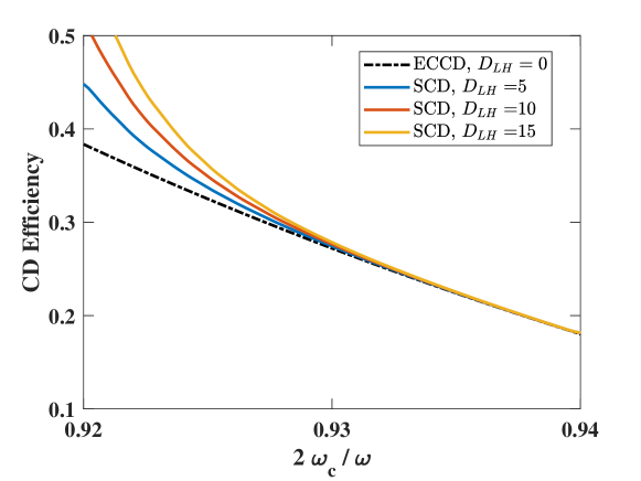
Figure 3: The SCD efficiency with different $D_{LH}$ based on fixed ECCD at $\theta_{p}=90^{\circ}$ and $n_{\parallel}=0.5$.

Fig.3 shows that the SCD efficiency increases with the increasing $D_{LH}$ for the fixed ECCD case, since a larger $D_{LH}$ (i.e., the LHW power) represents a larger perturbation response function $\tilde{\delta\chi}$ directly. In addition, it also implies a larger modification of distribution $f_{M}\phi$, which exists a limitation that the linear approximation is applicable. Therefore, the premise of low RF power density can be further clarified, the modification caused by LHW power is smaller than the Maxwell distribution, and the ECW power is smaller than the LHW power.

2.4 The results of the quasilinear simulation

To examine the accuracy of our linear model, we use a two dimension Fokker-Planck code[18] with the relativistic effect and the trapped effect to simulate ECCD and SCD, respectively, whose efficiencies are defined by

$$\xi_{ECCD}=\frac{j_{ECW}}{P_{ECW}},$$ (57)

$$\xi_{SCD}=\frac{j_{LHW+ECW}-j_{LHW}}{P_{ECW}}.$$ (58)

Due to the premise of low RF power density in the linear model, the diffusion coefficient of ECW, the width of parallel refractive index of ECW, and the diffusion coefficient of LHW are 0.01, 0.01, and 0.015, respectively, in the quasilinear simulation, which ensures that the RF powers are correspondingly small and the ECW power is smaller than the LHW power. The ion temperature is 1.5keV and the other plasma, magnetic and LHW parameters are the same with the linear case. We depict both CD situations as a function of $y$ at $\theta_{p}=0^{\circ}$. As shown in Fig.4, the results of the quasilinear simulation are consistent with those of the linear case in trends, both of which show the existence of the synergy effect at smaller $y$.

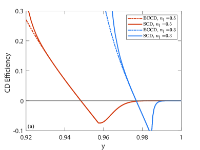
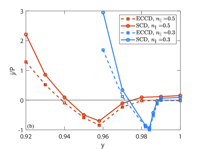
Figure 4: The comparison of the efficiency of SCD and ECCD between (a)the linear model and (b)the quasilinear simulation.

However, an important feature observed in the quasilinear simulation, which is not evident in the linear case, is that the SCD efficiency remains slightly higher than the ECCD efficiency, except for smaller values of $y$. There are two main reasons for this disagreement. One is that LHW power leads to an increase in ECW power deposition. Since the power deposition is associated with the diffusion coefficients in the quasilinear simulation, we change the diffusion coefficients of LHW and ECW with the same amplitude of 0.005, respectively, to distinguish the dependence of SCD on the power of LHW and ECW.

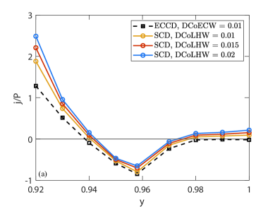
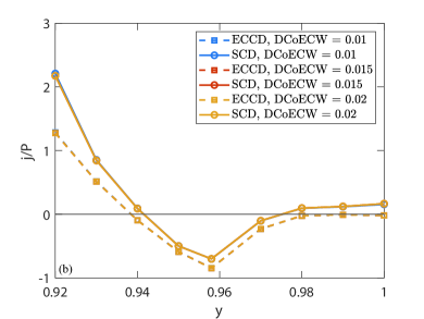
Figure 5: The CD situations with different diffusion coefficients at $\theta_{p}=0$ and $n_{\parallel}=0.5$. (a)DCoLHW and (b)DCoECW mean, respectively, diffusion coefficient of LHW and ECW.

As shown in Fig.5(a), with the increase of the diffusion coefficient of LHW, it indicates that not only the synergy effect is stronger with smaller $y$, which is consistent with the linear case manifested in Fig.3, but also the disagreement between the linear model and the quasilinear simulation becomes larger. In contrast, Fig.5(b) shows no obvious changes varying with the diffusion coefficient of ECW. In the presence of LHW, the ECW power deposition is increased slightly and additional driving current is generated, resulting in a larger $j_{LHW+ECW}$ term in Eq.(52). Since the ECW power $P_{ECW}$ adopted in Eq.(52) is the same as that in Eq.(51), $\xi_{SCD}$ is slightly larger than $\xi_{ECCD}$ except for smaller $y$. The other is due to the slowing-down process of high-energy electrons. We depict the electron distribution function in velocity space with the resonance curve of ECW at $y=0.99$ and $n_{\parallel}=0.5$ and the diffusion of LHW at the fixed velocity region from $3u_{e}$ to $5u_{e}$ to illustrate the impact of the slowing-down effect on SCD. As shown in Fig.6, where the resonance curve of ECW and the diffusion region of LHW exist, the localized electrons gain energy and increase the temperature, which is reflected in the modification of Maxwellian distribution.

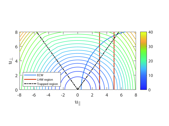
Figure 6: The electron distribution function in velocity space.

The distribution located at the diffusion region of LHW (the area between the two vertical orange lines) is modified in parallel velocity direction. The portion of ECW passing through (the blue line) is modified in vertical direction, and the distribution altered by ECW in the trapped region is symmetric due to the pitch-angle scattering. Those high-energy electrons in the trapped region pushed by ECW will go through the slow-downing process, although the probability of electrons escaping from both sides of the trapped region is equal, the electrons escaping on the right side can be further accelerated by LHW, resulting in asymmetric electrons relaxation in velocity space, and it causes the appearance of additional driving current. In addition, the asymmetric electrons relaxation also depends on the LHW power. Indeed, the synergy effect manifested by the quasilinear simulations except for smaller $y$, occurs indirectly through a non-linear process, which is not due to the overlap of the two waves’ quasilinear domains, so it is naturally different from the linear case.

3 The criteria of the synergy effect

The advantage of a linear model compared to simulations and experiments is that we are able to probe the criterion of occurring synergy effect. The synergy efficiency according to Eqs.(48) and (49) can be written as

$$\zeta_{syn}^{*}=-\frac{4}{\ln\Lambda}\langle\frac{B}{B_{m}}\rangle\frac{mu_{e}^{2}\int d\gamma(u_{\perp})^{2\ell}f_{M}\tilde{\Lambda}\tilde{\delta\chi}}{\int d\gamma(u_{\perp})^{2\ell}f_{M}},$$ (59)

Obviously, if the integral in numerator

$$mu_{e}^{2}\int(u_{\perp})^{2\ell}f_{M}\tilde{\Lambda}\tilde{\delta\chi}>0,$$ (60)

the synergy effect will occur. Here, the lower and upper bound of integral are $max\left[\gamma(u_{\parallel,1}),\gamma_{min}\right]$ and $min\left[\gamma(u_{\parallel,2}),\gamma_{max}\right]$, in which $\gamma(u_{\parallel,1})$ and $\gamma(u_{\parallel,2})$ represent $\gamma$ calculated by resonance relation $\delta(\gamma-\frac{n_{\parallel}u_{\parallel}}{c}-y)$ with the left boundary of LHW $u_{\parallel,1}$ and the right $u_{\parallel,2}$, and $\gamma_{min}$, $\gamma_{max}$ are the lower and upper bounds determined by Eq.(46). The reason that Eq.(53) can be considered as a criterion for the occurrence of synergy effect would be explained by the matching pattern of ECW’s resonance curves and LHW’s diffusion region in velocity space.

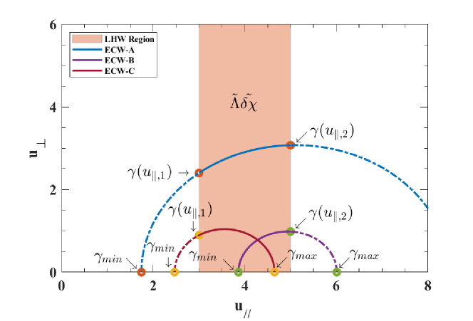
Figure 7: The resonance curves of ECW and the diffusion region of LHW in velocity space. The meaning of each point is marked in the figure. The different color lines denote different CD cases: ECW-A($y=0.95,n_{\parallel}=0.4$), ECW-B($y=0.92,n_{\parallel}=0.4$), and ECW-C($y=0.958,n_{\parallel}=0.3$). The LHW diffusion region is fixed at range of $3u_{e}$ to $5u_{e}$.

There are three typical situations in which resonance curves of ECW are located in velocity space without considering the trapped region, as shown in Fig.7. Each part in the criterion Eq.(53) has its own physical meaning in velocity space. $(u_{\perp})^{2\ell}$ gives lower $\gamma_{min}$ and upper $\gamma_{max}$ bounds and ensures that the integral is integrated along the resonance curve of ECW. The Maxwellian distribution $f_{M}$ represents that most electrons exist in the low-energy area instead of the high one. The perturbation response function $\tilde{\delta\chi}$ describes additional electron relaxation caused by LHW in a given region, and the operator $\tilde{\Lambda}$ acting on $\tilde{\delta\chi}$ results in a modified distribution, but $mu_{e}^{2}\tilde{\Lambda}\tilde{\delta\chi}$ wouldn’t appear outside of the given region. Thus the dashed line part of the resonance curve of ECW has no integral contribution to the synergy effect, and only the solid line part of the resonance curve can take effect. Correspondingly, the lower and upper bounds of integral change to $max\left[\gamma(u_{\parallel,1}),\gamma_{min}\right]$ and $min\left[\gamma(u_{\parallel,2}),\gamma_{max}\right]$ as illustrated in Tab.2.

Table 2: The bounds of the integral in different cases.

Case	lower bound	upper bound
ECW-A	$\gamma(u_{\parallel,1})$	$\gamma(u_{\parallel,2})$
ECW-B	$\gamma_{min}$	$\gamma(u_{\parallel,2})$
ECW-C	$\gamma(u_{\parallel,1})$	$\gamma_{max}$

The reason we neglect the trapped effect is that the synergy effect tends to occur directly in the low energy part of the diffusion region of LHW, where the resonance curve of ECW is far from the trapped region. If the trapped boundaries at a given poloidal angle cross ECW’s resonance curve in LHW’s diffusion region, the resulting modification only changes the left bound of the integral. Considering there are fewer electrons in the high-energy area, the resonance curve of the remaining ECW makes a small contribution to the integral, even if the synergy effect occurs it will be very inconspicuous.

Additionally, although the criterion is established by Eq.(53), the synergy effect still can be insignificant due to the larger denominator in Eq.(52). We introduce two new definitions

$$\kappa=mu_{e}^{2}\int_{max\left[\gamma(u_{\parallel,1}),\gamma_{min}\right]}^{min\left[\gamma(u_{\parallel,2}),\gamma_{max}\right]}d\gamma(u_{\perp})^{2\ell}f_{M}\tilde{\Lambda}\tilde{\delta\chi}\bigg{/}\int_{max\left[\gamma(u_{\parallel,1}),\gamma_{min}\right]}^{min\left[\gamma(u_{\parallel,2}),\gamma_{max}\right]}d\gamma(u_{\perp})^{2\ell}f_{M},$$ (61)

and

$$\eta=\int_{max\left[\gamma(u_{\parallel,1}),\gamma_{min}\right]}^{min\left[\gamma(u_{\parallel,2}),\gamma_{max}\right]}d\gamma(u_{\perp})^{2\ell}f_{M}\bigg{/}\int_{\gamma_{min}}^{\gamma_{max}}d\gamma(u_{\perp})^{2\ell}f_{M},$$ (62)

where $\eta$ is the power factor that represents the ECW power deposited in the diffusion region of LHW divided by the total ECW power deposition, i.e., the integral represented by the solid part of the resonance curve of ECW divided by the integral represented by the total (solid + dashed part) resonance curve of ECW, and $\kappa$ is the CD efficiency of the ECW power deposited in the diffusion region of LHW. Therefore, the synergy efficiency reads

$$\zeta^{*}_{syn}=-\frac{4}{\ln\Lambda}\langle\frac{B}{B_{m}}\rangle\kappa\eta.$$ (63)

Obviously, the final magnitude of the synergy effect is determined by $\kappa$ and $\eta$ together at a given flux surface. Actually, $\eta$ quantifies the degree of the overlap of the two waves’ quasilinear domains, we consider the criterion that the synergy effect is sufficiently significant in the numerical calculation as

$$\eta>1\times 10^{-4}.$$ (64)

We depict $\tilde{\zeta}_{syn}$ varying with $y$ and mark threshold values of the two criteria as shown in Fig.8, the parameters are the same with Tab.1 except for $n_{\parallel}=0.3,0.4,0.5$. The specific threshold values of $y$ corresponding to the marked points in Fig.8 are shown in Tab.3.

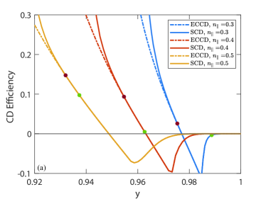
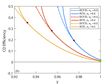
Figure 8: The points of criteria are marked at different poloidal angles (a)$\theta_{p}=15^{\circ}$ and (b)$\theta_{p}=165^{\circ}$. The green and red points determined by Eq.(54) and Eq.(58), respectively, represent the threshold values of occurrence and sufficient significance of the synergy effect.

Table 3: The specific threshold values of occurrence and sufficient significance of the synergy effect.

$\theta_{p}=15^{\circ}$	$n_{\parallel}=0.3$	$n_{\parallel}=0.4$	$n_{\parallel}=0.5$
Point	y	y	y
Green	0.9887	0.9627	0.9373
Red	0.9760	0.9547	0.9307

$\theta_{p}=165^{\circ}$	$n_{\parallel}=0.3$	$n_{\parallel}=0.4$	$n_{\parallel}=0.5$
Point	y	y	y
Green	1	1	1
Red	0.9800	0.9587	0.9373

The above data manifest that the high-field side of a flux surface has a broader $y$ scope for the synergy effect, and it is significant enough only when the power factor is larger than $0.01\%$. The reason why the synergy effect is inclined to take place at the high-field side of a given flux surface instead of the weak-field side is that the trapped region of the former is smaller and relatively there are more passing electrons. In general, the two criteria imply that the synergy effect quantitatively depends on the power factor $\eta$, the constant $D_{LH}$ determined by the LHW power, and the synergy electrons.

Optimizing the synergy effect requires improvements in above three aspects by combing practical experimental conditions. The power factor $\eta$ is a function of several variables including $y$, $n_{\parallel}$, $u_{\parallel,1}$, $u_{\parallel,2}$, and $T_{e}$. Among these variables, $y$ and $n_{\parallel}$ influence the shape of the resonance curve of ECW, while $u_{\parallel,1}$ and $u_{\parallel,2}$, determined by Landau damping, extract the relevant portion contributing to the synergy effect. It is worth noting that the integral $\int_{\gamma_{min}}^{\gamma_{max}}d\gamma(u_{\perp})^{2\ell}f_{M}$ is non-linear along the resonance curve due to the exponential decrease of $f_{M}$ as $\gamma$ increases. Consequently, the low-energy part (i.e., the smaller $\gamma$) of the resonance curve contributes more significantly compared to the high-energy part (i.e., the larger $\gamma$). Therefore, optimizing $\eta$ involves maximizing the involvement of the low-energy portion of the resonance curve of ECW within the diffusion region of LHW by appropriately adjusting the parameters of $\eta$. On the other hand, the constant $D_{LH}$, determined by the LHW power, directly affects the magnitude of $\tilde{\delta\chi}$ that represents the degree of electron relaxation induced by LHW power in velocity space. Hence, increasing the LHW power within the limitations of the linear model is beneficial for enhancing the synergy effect. Finally, the aforementioned optimizations imply that synergy electrons, which are electrons that undergo continuous acceleration and acquire higher energies, serve as the primary contributors to the overall synergy effect, thus more synergy electrons will make the synergy effect performing stronger.

Although we can not use quasilinear simulation to cross-validate the two criteria due to the nonlinear nature of simulation, both criteria still show great application potential for quickly determining whether the synergy effect occurs and whether it’s significant enough for given parameters.

4 Summary

A linear model of SCD with LHW and ECW has been presented in this paper. The SCD efficiency compared to the ECCD efficiency is given in parameters space, and the comparison results show that the synergy effect is inclined to occur at smaller $y=2\omega_{c}/\omega$ with the fixed $n_{\parallel}$ and $\theta_{p}$. We examine the accuracy of the linear model with quasilinear simulation using a 2D Fokker-Planck code, the linear and quasilinear results of CD’s efficiency are consistent in trends at the premise of low RF power density, and the disagreement except for smaller $y$ is due to the natural differences of quasilinear simulation and linear model, the former includes the synergy effect that occurs indirectly through slowing-down process, but the later only reflects the synergy effect that occurs directly through the overlap of the waves’ quasilinear domains. Two criteria for the occurrence and the sufficient significance of the synergy effect are proposed, which correspond to Eq.(54) and Eq.(58), respectively. The criteria indicate that the synergy effect is dependent on the power factor of ECW, the LHW power, and synergy electrons, which can quickly determine its magnitude.

This study presents a quantitative analysis of the synergy effect. Previous understanding of this effect remains qualitative, focusing on electrons being pushed by ECW into the diffusion region of LHW, where they are further accelerated to become synergy electrons. By considering the direct mechanism of SCD, the process of continuously gaining energy for electrons necessitates the overlap of power deposition in radial location and quasilinear domains in velocity space of LHW and ECW. Our linear model indicates key physical quantities that quantify the degree of both overlap, namely the constant $D_{LH}$ and the power factor $\eta$. The constant $D_{LH}$, determined by LHW power, measures the extent of the overlap of the LHW power deposition in radial location. The power factor $\eta$, defined as the ratio of ECW power deposited in the diffusion region of LHW to total ECW power deposition, quantifies the degree of overlap in their quasilinear domains in velocity space. Additionally, the overlap excites electrons into synergy electrons, which serve as primary contributors to the synergy effect. In general, the linear model offers a quantitative description of SCD.

It should be mentioned that this linear model is universally applicable to other relevant parameters and shows the potential for application in ray-tracing code, which is conducive to real-time control of experimental plasma. Besides, the theoretical formulation of the above calculations also displays the possibility of generalizing application to other synergetic CD based on the matching pattern of quasilinear domains in velocity space.

Appendix A Lin-Liu’s formulations

The zero-order response function given by Lin-Liu is

$$\tilde{\chi}_{0}=sgn(u_{\parallel})F(u)H(\lambda),$$ (65)

where

$$F(u) =\frac{1}{f_{c}u_{e}^{4}}\left(\frac{\gamma+1}{\gamma-1}\right)^{\hat{\rho}/2}\int_{0}^{u}du^{\prime}\left(\frac{u^{\prime}}{\gamma^{\prime}}\right)^{3}\left(\frac{\gamma^{\prime}-1}{\gamma^{\prime}+1}\right)^{\hat{\rho}/2}$$ (66)

$$=\frac{1}{f_{c}}\left(\frac{u^{4}}{u_{e}^{4}}\right)\int_{0}^{1}dxx^{\hat{\rho}+3}\frac{1}{\left(1+(ux/c)^{2}\right)^{3/2}}$$ (67)

$$\quad\times\left[\frac{1+\sqrt{1+(u/c)^{2}}}{1+\sqrt{1+(ux/c)^{2}}}\right]^{\hat{\rho}},$$ (68)

and

$$H(\lambda)\equiv\frac{\theta(1-\lambda)}{2}\int_{\lambda}^{1}\frac{d\lambda^{\prime}}{\left\langle\left(1-\lambda^{\prime}B/B_{m}\right)^{1/2}\right\rangle}.$$ (69)

Here $\hat{\rho}\equiv\frac{Z_{\mathrm{eff}}+1}{f_{c}}$ and $f_{c}$ is the effective circulating particles fraction in the neoclassical transport theory, which is determined by

$$f_{c} \equiv\frac{3}{2}\left\langle\frac{B^{2}}{B_{m}^{2}}\right\rangle\int_{0}^{1}d\lambda H(\lambda)$$ (70)

$$=\frac{3}{4}\left\langle\frac{B^{2}}{B_{m}^{2}}\right\rangle\int_{0}^{1}\frac{\lambda d\lambda}{\left\langle\left(1-\lambda B/B_{m}\right)^{1/2}\right\rangle}.$$ (71)

Appendix B The approximation of $F(u)$

We suppose the relativistic $F(u)$, whose specific form is Eq.(A.2), and its derivatives can be approximated as simple functions with fixed order for the convenience of numerical calculation. In our calculations, we use mathematica to fit $F(u)$, which is

$$F(u)=(\frac{u}{u_{e}})^{3.1214}$$ (72)

with $C_{k}=1$ and $k=3.1214$. The numerical results of the two functions Eq.(A.2) and Eq.(B.1), and their derivatives are shown in Fig.B1. The blue, orange, and yellow lines denote, $F(u)$ itself, the first order derivative $\partial F(u)/\partial u$, and the second order derivative $\partial^{2}F(u)/\partial u^{2}$, respectively. The solid line representing Eq.(B.1) is close enough to the dashed line representing Eq.(A.2).

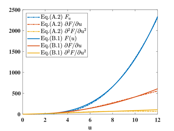
Figure 9: The numerical differences between Eq.(A.2)(dashed lines) and Eq.(B.1)(solid lines).

Then we calculate the statistical correlation between dashed and solid lines, as shown in Tab.B1.

Table 4: Statistical correlation analysis between Eq.(A.2) and Eq.(B.1).

	Root mean square error	Correlation coefficient	P-value
$F(u)$	15.167617	0.999839	0
$\partial F(u)/\partial u$	13.545415	0.997474	0
$\partial^{2}F(u)/\partial u^{2}$	12.370348	0.938761	0

The above data show that $F(u)$ itself and its first derivative $\partial F(u)/\partial u$ have strong statistical correlation between Eq.(A.2) and Eq.(B.1). Although the statistical correlation of second derivative $\partial^{2}F(u)/\partial u^{2}$ is poor, considering the small contribution of higher-order derivative in differential equation Eq.(29), the above numerical approximation is still valuable and $F(u)$ Eq.(B.1) can be taken in following derivations for the convenience of calculation.

Appendix C The interpolation formulation of $E(\lambda)$

The useful interpolation formulations about $E(\lambda)$ and its first derivative are

$$E(\lambda)=\frac{\theta(1-\lambda)}{2}(1-h_{1})^{1/2}\int_{s}^{1}dz\frac{\left[k(1-h_{1})+3h_{1}z\right]}{(1-h_{1}+zh_{1})^{5/2}\left[1+z^{2}(c_{2}(1-z^{2})+c_{4}z^{2})\right]^{1/2}},$$ (73)

and

$$\frac{dE(\lambda)}{d\lambda}=-\frac{1}{2}\frac{k-(k-3)\lambda h_{1}}{(1-\lambda h_{1})^{1/2}\left[1+s^{2}(c_{2}(1-s^{2})+c_{4}s^{2})\right]^{1/2}}.$$ (74)

Here, $s=\lambda(1-h_{1})/(1-\lambda h_{1})$ and coefficients are

$$c_{2}=-\frac{1}{4}\frac{(\langle h^{2}\rangle-\langle h\rangle^{2})}{(1-\langle h\rangle)^{2}},$$ (75)

$$c_{4}=\frac{\left\langle(1-h)^{1/2}\right\rangle^{2}}{(1-\langle h\rangle)}-1.$$ (76)

The three flux-surface averaged quantities can be written as

$$\langle h\rangle=1-\varepsilon,$$ (77)

$$\langle h^{2}\rangle=\frac{(1-\varepsilon)^{2}}{(1-\varepsilon)^{1/2}},$$ (78)

$$\left\langle(1-h)^{1/2}\right\rangle=\frac{1}{\pi}\left[(1+\varepsilon)\sin^{-1}\sqrt{\frac{2\varepsilon}{1+\varepsilon}}+\sqrt{2\varepsilon(1+\varepsilon)}\right].$$ (79)

By definition $E(\lambda)\equiv D_{k}(\lambda)M(\lambda)$, the interpolation form of $M(\lambda)$ is

$$M(\lambda)=\frac{\theta(1-\lambda)}{2}\frac{(1-h_{1})^{1/2}}{k-(k-3)\lambda h_{1}}$$ (80)

$$\times\int_{s}^{1}dz\frac{(k(1-h_{1})+3zh_{1})}{(1-h_{1}+zh_{1})^{5/2}\left[1+z^{2}(c_{2}(1-z^{2})+c_{4}z^{2})\right]^{1/2}}.$$ (81)

References

References

- [1] N.J. Fisch 1987 Rev. Mod. Phys.59 175
- [2] I.Fidone et al1984 \PF27 2468
- [3] I.Fidone et al1987 \NF27 579
- [4] G.Giruzzi et al2004 Phys. Rev. Lett.93 255002
- [5] A.Polevoi et al2008 \NF48 015002
- [6] Jinping Qian et al2016 \PST18 457
- [7] R. Dumont et al2000 Phys. Plasmas 7 3449
- [8] R.J. Dumont et al2004 Phys. Plasmas 11 3449
- [9] R.H. Cohen 1988 \PF30 2442 (1987); 31 421.
- [10] Y.R.Lin-Liu et al2003 Phys. Plasmas 10 4064
- [11] D.W. Ignat et al1994 \NF34 837
- [12] D.B. Batchelor and R. C. Goldfinger 1982 Report ORNL/TM-6844
- [13] A.P. Smirnov and R.W. Harvey, Bull. Am. Phys. Soc. 40 1837
- [14] S. Y. Chen et al2012 Plasma Phys. Control. Fusion54 115002
- [15] P.W. Zheng et al2019 \NF59 054003
- [16] T.M. Antonsen and K.R. Chu 1982 \PF25 1295
- [17] N.J. Fisch 1981 Phys. Rev.A 24 3245
- [18] Y. Peysson and M. Shoucri 1998 \CPC109 55
- [19] Y.R. Lin-Liu and R.L. Miller 1995 Phys. Plasmas 2 1666
- [20] M. Taguchi 1983 J. Phys. Soc. Japan52 2035
- [21] J, Huang et al2014 Phys. Plasmas 21 012508
- [22] C.C. Petty et al2002 \NF42 1366