Exploiting Multiple Priors for Neural 3D Indoor Reconstruction

Abstract

Neural implicit modeling permits to achieve impressive 3D reconstruction results on small objects, while it exhibits significant limitations in large indoor scenes. In this work, we propose a novel neural implicit modeling method that leverages multiple regularization strategies to achieve better reconstructions of large indoor environments, while relying only on images. A sparse but accurate depth prior is used to anchor the scene to the initial model. A dense but less accurate depth prior is also introduced, flexible enough to still let the model diverge from it to improve the estimated geometry. Then, a novel self-supervised strategy to regularize the estimated surface normals is presented. Finally, a learnable exposure compensation scheme permits to cope with challenging lighting conditions. Experimental results show that our approach produces state-of-the-art 3D reconstructions in challenging indoor scenarios.

1 Introduction

Recent developments in neural implicit representation strategies permit to build dense geometric models of scenes. These techniques can not only produce continuous representations, but they also exhibit very promising results in contexts very challenging for traditional 3D reconstruction methods, e.g., texture-less areas. Among these models, NeRF-based approaches, enhanced with more stringent geometrical constraints, showed impressive results on the 3D reconstruction of object-centric scenes [Niemeyer et al.(2020)Niemeyer, Mescheder, Oechsle, and Geiger, Yariv et al.(2020)Yariv, Kasten, Moran, Galun, Atzmon, Ronen, and Lipman, Oechsle et al.(2021)Oechsle, Peng, and Geiger]. However, the geometry estimation of fine structures is still challenging due to the nature of implicit representation models which tend to ignore high frequency details. Many NeRF-based solutions rely on geometry cues from depth sensors or external methods to guide the reconstruction [Roessle et al.(2022)Roessle, Barron, Mildenhall, Srinivasan, and Nießner, Azinović et al.(2022)Azinović, Martin-Brualla, Goldman, Nießner, and Thies] but, in these cases, the results are strongly dependent on the quality of the geometrical hints. Furthermore, these methods struggle on larger and indoor scenes, due to the higher geometry complexity. In such scenarios, acquisitions may capture regions at different scales and focus on many complex structural details. Moreover, in real scenarios, brighter or darker regions of the scene can cause the camera exposure to change significantly: this results in the same subject exhibiting very different colors across different images.

In this work, we present a NeRF-based method which learns an implicit representation of indoor environments and produces accurate 3D reconstructions. Our method exploits external depth priors and a novel self-supervised normal regularization. In particular, we introduce a soft depth supervision which suggests to the model the geometry of the scene indirectly, by optimizing the sampling procedure. Moreover, we regularize the surfaces through a self-supervised strategy which exploits spatial information available in the input images that are first pre-processed by a learnable exposure compensation scheme. Reconstruction results outperform competing methods on the 3D reconstruction of indoor scenes.

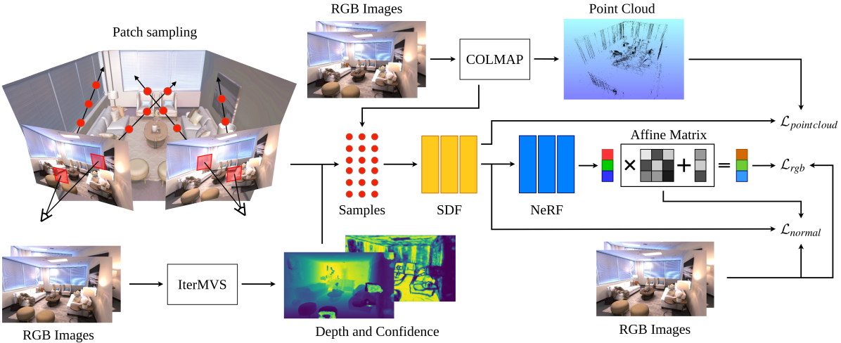
Figure 1: Overview of the proposed approach.

2 Related Work

In recent years, neural implicit representations [Chen and Zhang(2019)] have gained popularity and have spread across many different domains [Michalkiewicz et al.(2019)Michalkiewicz, Pontes, Jack, Baktashmotlagh, and Eriksson, Dupont et al.(2021)Dupont, Goliński, Alizadeh, Teh, and Doucet, Yüce et al.(2022)Yüce, Ortiz-Jiménez, Besbinar, and Frossard, Peng et al.(2021)Peng, Zhang, Xu, Wang, Shuai, Bao, and Zhou, Strümpler et al.(2022)Strümpler, Postels, Yang, Gool, and Tombari, Saragadam et al.(2022)Saragadam, Tan, Balakrishnan, Baraniuk, and Veeraraghavan]. Geometry reconstruction is one of the fields that has benefited the most from these approaches. Traditional explicit representation for 3D scenes, like voxel grids [Gadelha et al.(2017)Gadelha, Maji, and Wang, Jimenez Rezende et al.(2016)Jimenez Rezende, Eslami, Mohamed, Battaglia, Jaderberg, and Heess], point clouds [Achlioptas et al.(2018)Achlioptas, Diamanti, Mitliagkas, and Guibas, Camuffo et al.(2022)Camuffo, Mari, and Milani] or meshes [Kato et al.(2018)Kato, Ushiku, and Harada, Wang et al.(2018)Wang, Zhang, Li, Fu, Liu, and Jiang] have some drawbacks, such as the high memory footprint, the fixed resolution and their discrete nature.

Implicit representations aim at solving many of the above mentioned limitations. They can represent a continuous volume, so the extraction of explicit models at any resolution becomes possible. Moreover, they drastically reduce the required memory footprint. In the field of 3D representations, the first proposed solutions represented the volume exploiting Signed Distance Fields (SDFs) [Park et al.(2019)Park, Florence, Straub, Newcombe, and Lovegrove, Zhang et al.(2021)Zhang, Yao, and Quan] or occupancy grids [Mescheder et al.(2019)Mescheder, Oechsle, Niemeyer, Nowozin, and Geiger, Oechsle et al.(2021)Oechsle, Peng, and Geiger]. SDF suddenly became the choice for many works aimed at obtaining accurate geometry reconstruction of objects or scenes due to its differentiable nature. Recently, new solutions based on parametric encodings have been published, showing impressive results [Müller et al.(2022)Müller, Evans, Schied, and Keller, Chen et al.(2022)Chen, Xu, Geiger, Yu, and Su, Chen et al.(2023)Chen, Xu, Wei, Tang, Su, and Geiger, Wang et al.(2022c)Wang, Han, Habermann, Daniilidis, Theobalt, and Liu]. The idea is to learn the SDF by substituting the network or enhancing its capability through local parameters stored in multi-resolution data structures. At the price of a higher memory footprint, these approaches can improve the reconstruction quality and reduce the training time.

In the literature there are examples of methods exploiting external geometrical clues [Yu et al.(2022)Yu, Peng, Niemeyer, Sattler, and Geiger, Wang et al.(2022b)Wang, Wang, Long, Theobalt, Komura, Liu, and Wang, Atzmon and Lipman(2020), Roessle et al.(2022)Roessle, Barron, Mildenhall, Srinivasan, and Nießner] to guide the reconstruction. Knowing in advance the depth or the normal of some surface points adds strong constraints that help the model to converge faster and to estimate a better geometry. These priors could come from depth sensors [Zanuttigh et al.(2016)Zanuttigh, Marin, Dal Mutto, Dominio, Minto, and Cortelazzo] or they may be estimated through monocular or Multi-View Stereo (MVS) methods [Wang et al.(2022a)Wang, Galliani, Vogel, and Pollefeys, Sormann et al.(2021)Sormann, Rossi, Kuhn, and Fraundorfer]. Other approaches exploit point clouds from Structure-from-Motion (SfM) approaches for supervision: the SDF estimation can be guided by these point clouds [Deng et al.(2022)Deng, Liu, Zhu, and Ramanan, Fu et al.(2022)Fu, Xu, Ong, and Tao] or it is possible to initialize a per-point feature vector encoding color and density information [Xu et al.(2022)Xu, Xu, Philip, Bi, Shu, Sunkavalli, and Neumann].

There exist also SDF-based methods explicitly targeting indoor scenes: specifically, NeuRIS [Wang et al.(2022b)Wang, Wang, Long, Theobalt, Komura, Liu, and Wang] is a recent method that employs monocular normal maps to guide the reconstruction relying also on a patch-match regularization strategy; MonoSDF [Yu et al.(2022)Yu, Peng, Niemeyer, Sattler, and Geiger] leverages the information in monocular depth maps in addition to normal maps to enforce stronger geometrical constraints. With respect to these methods, our approach exploits external priors by proposing a depth map soft supervision which focuses the sampling on the area closer to the surface without introducing a direct supervision. Furthermore, the proposed normal self regularization acts as smoothing constraint without the need for external normal maps that are often inaccurate in challenging scenarios. Finally, a revised exposure compensation approach improves the results in challenging lighting conditions, typical of indoor scenes.

3 Method

The goal of this work is to reconstruct the geometry of complex indoor environments starting from RGB images only. Previous SDF-based approaches for the task, like NeuS [Wang et al.(2021)Wang, Liu, Liu, Theobalt, Komura, and Wang] and IDR [Yariv et al.(2020)Yariv, Kasten, Moran, Galun, Atzmon, Ronen, and Lipman], focus on learning the geometry and the appearance of object-centric scenes. We introduce new supervision and regularization strategies to improve the reconstruction accuracy of larger scenes. More in detail, we propose two depth-based supervision strategies exploiting sparse and dense depth priors, respectively (Sec. 3.3). Furthermore, we introduce a strategy to handle variable exposure settings (Sec. 3.2) and a self-supervised method to regularize the surface normals (Sec. 3.4).

3.1 Neural Implicit Surface Rendering

Scene Representation

The geometry is represented using the Signed Distance Function (SDF). This is a function $f:\mathbb{R}^{3}\to\mathbb{R}$ that assigns to every point in the volume the distance between this point and the closest surface in the scene. Consequently, the scene surface $\mathcal{S}$ is the set of 3D coordinates with SDF value equal to 0: formally it is $\mathcal{S}=\left\{x\in\mathbb{R}^{3}|f\left(x\right)=0\right\}$.

Moreover, the radiance field is represented as a function $c:\mathbb{R}^{3}\times\mathbb{S}^{2}\to\mathbb{R}^{3}$ that assigns to every 3D point a color depending on the camera viewing direction, with $\mathbb{S}^{2}$ defined as $\mathbb{S}^{2}=\left\{x\in\mathbb{R}^{3}:\lVert x\rVert=1\right\}$. The functions $f$ and $c$ are modeled by a couple of Multi-Layer Perceptrons (MLPs).

Volume Rendering

Since the aim of this work is accurate geometry reconstruction, we follow the common volume rendering solution but substituting the density term with a more geometrically constrained one, called opacity $\rho$. Following the parameterization proposed in NeuS [Wang et al.(2021)Wang, Liu, Liu, Theobalt, Komura, and Wang], this term is a function of the Sigmoid computed at the SDF values. This formulation is unbiased and occlusion aware, making the method better suited for 3D Reconstruction. Once the opacity is computed, the rendering procedure is the same as in the original NeRF [Mildenhall et al.(2020)Mildenhall, Srinivasan, Tancik, Barron, Ramamoorthi, and Ng]. All the colors and opacities along each ray are summed up to produce the final color according to the following relation:

$$C(\mathbf{o},\mathbf{v})=\int_{0}^{+\infty}w(t)c(\mathbf{p}(t),\mathbf{v})\,dt$$ (1)

where $\mathbf{o}$ is the position of the camera, $\mathbf{v}$ the viewing direction, $\mathbf{p}=\mathbf{o}+t\mathbf{v}$ the 3D point and $c$ and $w$ the color and the weight at each specific coordinate, respectively. The weight term is defined as $w(t)=T(\rho(t))\rho(t)$, with $T$ representing the accumulated transmittance. We refer the reader to NeuS [Wang et al.(2021)Wang, Liu, Liu, Theobalt, Komura, and Wang] for further details.

3.2 Variable Exposure Compensation

While object-centric scenes considered in previous approaches exhibit uniform illumination, larger indoor scenes often have many light variations and are often acquired with variable camera exposure settings. In order to compensate for the differences in colors coming from the non-constant exposure and white balancing, inspired by the method proposed in [Rematas et al.(2022)Rematas, Liu, Srinivasan, Barron, Tagliasacchi, Funkhouser, and Ferrari], we introduce an exposure compensation strategy based on an affine model. In particular, an affine transformation is learned for each training image and applied to the RGB color produced by the rendering network before comparing it with the ground truth.

Differently from [Azinović et al.(2022)Azinović, Martin-Brualla, Goldman, Nießner, and Thies, Martin-Brualla et al.(2021)Martin-Brualla, Radwan, Sajjadi, Barron, Dosovitskiy, and Duckworth], we do not employ ad-hoc compensation networks to avoid an over-parameterization of the model [Rematas et al.(2022)Rematas, Liu, Srinivasan, Barron, Tagliasacchi, Funkhouser, and Ferrari] and we directly optimize the 12 parameters of the affine transformation. Therefore, the rendered color $C_{k}(p)$ for pixel $p$ in image $k$ is:

$$C_{k}(p)=R_{k}\hat{C}_{k}(p)+\mathbf{t}_{k}\quad\text{with}\quad A_{k}=[R_{k}|\mathbf{t}_{k}]$$ (2)

where $\hat{C}_{k}(p)$ is the output of the rendering network. The parameters are initialized with $R_{k}=I$ and $\mathbf{t}_{k}=\mathbf{0}$. Such an initialization scheme is an initial strong prior but it is reasonable since the real colors are not too far from the acquired ones. Furthermore, in order to avoid the convergence to unexpected color shifts, we introduce an anchor point. In particular, the matrix, corresponding to the reference image chosen among the ones with the most uniform color histogram, is fixed to the initialization values. In this way, the affine matrices corresponding to all the other images are forced to produce a color appearance resembling that of the reference image, thus aligning the exposure settings of the whole scene.

3.3 Depth Supervision

Since our model relies exclusively on RGB images, we propose to exploit geometry information retrieved from the same RGB pictures used as input. Such supervision is beneficial since it supports the SDF network training by adding reliable geometrical constraints that improve the results and a guidance for the sampling stage to speed-up the training. Querying the SDF model permits producing information about the depth value for each pixel, that can be compared with depth data retrieved from RGB images through other strategies.

We implement two synergic supervision strategies: a point cloud supervision, exploiting sparse depth data, and a depth map soft supervision, employing dense depth data.

Sparse Pointcloud Supervision

One approach, similar to DS-NeRF [Deng et al.(2022)Deng, Liu, Zhu, and Ramanan], exploits the sparse point cloud produced by the SfM algorithm during the camera pose estimation. In our setting we use COLMAP [Schönberger et al.(2016)Schönberger, Zheng, Pollefeys, and Frahm, Schönberger and Frahm(2016)]. Generally, these 3D points (denoted keypoints) are sparse but reliable, since they are the result of a robust feature extraction and triangulation procedure. For this purpose, it is possible to consider the rays passing through the point cloud keypoints seen by the current camera [Deng et al.(2022)Deng, Liu, Zhu, and Ramanan]. At this point, the weights $w$ of the points along the ray are used to estimate a depth value as follows:

$$\hat{D}(r)=\int_{t_{n}(r)}^{t_{f}(r)}w(t)tdt$$ (3)

where $r$ is the considered ray, $t_{n}(r)$ and $t_{f}(r)$ the near and far Region of Interest (RoI) bounds along the considered ray, respectively, and $t$ the distance of that sample from the camera position. This permits to define a loss $\mathcal{L}_{pc}$ that compares the depth $\hat{D}$ rendered by the model against the depth $D$ predicted by COLMAP.

It is important to notice that the produced point cloud is sparse therefore, when projected on the current camera image plane, most of pixels do not observe a keypoint. Considering that each pixel of an image may be chosen to cast a ray, this kind of supervision could be rarely applicable. For this reason, we choose to implement the supervision in parallel with the standard NeRF pipeline: we randomly cast a batch of rays for the main pipeline and a different batch of rays through the pixels observing a keypoint. These two batches are processed independently. Finally, we choose to consider only keypoints seen by at least a minimum number of different cameras, for better robustness.

Depth Map Soft Supervision

The point cloud supervision is effective in supporting the geometry estimation, but it is based on sparse data. Usually, less than 1000 valid keypoints are available for each camera, hence the majority of the rays is not supervised by the point cloud. For this reason, the next step aims at implementing a supervision that is available at any pixel. We adopt an approach exploiting depth and confidence maps generated by IterMVS [Wang et al.(2022a)Wang, Galliani, Vogel, and Pollefeys], a deep-learning algorithm for MVS depth map estimation. The main idea behind this approach is to exploit this depth information to focus the sampling only in the region close to the surface. To achieve this goal, a novel soft supervision strategy is presented. It is based on a Probability Distribution Function (PDF), built on the SDF weights $w$, which expresses the probability to encounter a surface at each step along a ray.

In the first phase, the NeuS original coarse-to-fine sampling is performed, in order to produce a PDF $h(x)$ which locates the estimated surfaces along the ray. This PDF is the result of the interpolation of the weights $w$ along the ray. At this point, according to depth information acquired from depth maps, a Gaussian PDF $n(x)=\mathcal{N}(d,\sigma)$ is generated. This is centered at the depth values $d$ and has standard deviation $\sigma$ proportional to the confidence $\mu$ of depth estimation. This PDF is combined with the PDF estimated by the SDF network:

$$g(x)=h(x)n(x)=h(x)\mathcal{N}(d,\sigma)\;\;\;\;\mathrm{with}\;\;\;\;\sigma=0.5(1-\mu).$$ (4)

Note that, if the two PDFs are independent, the product represents the joint probability. In our case, $h(x)$ is the probability of finding a surface along a ray, while $n(x)$ can be seen as the probability that the estimated depth is coherent with the depth map. Moreover, they come from different computations, so they can be considered independent.

Finally, all previous points are discarded and the new PDF $n(x)$ is used to re-sample less but more relevant new points, which will be used for the rendering pipeline (see Fig. 3). More in detail, half of these points (marked with “$\circ$” in the example of Fig. 3) are sampled according to $g(x)$, the second half is sampled linearly along the ray (“$\diamond$” in the figure). This permits an accurate sampling close to the surface for increased precision, and a coarse sampling on all the ray to handle critical cases where the current surface is wrong.

As a final consideration, in principle, the depth maps could be used to define an explicit loss, as done for the point cloud supervision. We evaluated this option: however since the depth information from these maps is generally less accurate, employing an explicit loss would lead to instability during the training, with different depth supervisions pulling towards different directions. For this reason, we choose to keep the more reliable depth supervision on point clouds and employ depth maps only to guide the sampling.

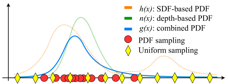
Figure 2: Depth map guided sampling strategy.

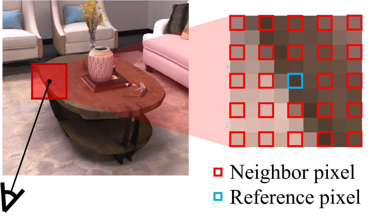
Figure 3: Normal regularization.

3.4 Normal Self Regularization

Even if both depth supervisions are effective in adding a reliable guidance to the geometry estimated by the SDF, it may happen that texture-less planar surfaces are not reconstructed as smooth as expected. This can be explained considering that COLMAP and IterMVS struggle to extract and triangulate reliable features on texture-less areas, leading to a lack of supervision in those regions.

To address this problem, we present a novel normal self regularization strategy. The idea is to guide the geometry estimation without using external normal priors, generally costly to compute and not always reliable. In our implementation, the model exploits both the information available in RGB images and in depth data. In the standard setting, at every iteration, sparse random pixels are sampled: however, this does not permit to exploit the spatial consistency due to the sparsity of the rays. Our solution consists in considering patches of pixels instead of single sparse pixels, and to cast a batch of rays for every patch, thus exploiting spatial information. The rationale is that close pixels with a similar color should represent surface points of a common plane [Rossi et al.(2020)Rossi, Gheche, Kuhn, and Frossard]. Otherwise, when the color is different, we cannot make any assumption on the geometry. This idea is implemented by computing for every pixel representing a surface point the surface normal, the surface depth and a weight. The depth is computed as described in Eq. 3, while the surface normal can be estimated as the gradient of the SDF in that specific point:

$$\hat{N}(r)=\int_{t_{n}(r)}^{t_{f}(r)}w(t)\nabla\mathbf{p}(t)dt$$ (5)

where $r$ is the considered ray, $t_{n}$ and $t_{f}$ the near and far RoI bounds and $t$ the distance of that sample from the camera position. Then, as shown in Fig. 3, we consider the central pixel of every patch as the reference and compute the weights $w_{b}$ quantifying the likelihood that one surface point belongs to the same plane of the central one, similarly to a bilateral filter:

$$w_{b}(r)=\mathcal{N}(I(i)-I(j),\sigma_{c})\mathcal{N}(\hat{P}(i)-\hat{P}(j),\sigma_{d})$$ (6)

where $\mathcal{N}$ is the normal distribution while $I$ is the pixel color corrected with the respective exposure compensation matrixes of Sec. 3.2 and converted to the CIE Lab color space to better capture the color similarity. Finally, $P$ are the 3D coordinates of the surface point and $i$ and $j$ the neighbor and reference pixels, respectively. The bilateral weights are computed considering the difference in color and in the actual location in the scene of two surface points. Therefore, the model can regularize wide surfaces while preserving edges and high frequency details. At this point, it is possible to force the surface normals to be similar to the central point surface normal according to the respective bilateral weight. The spatial term is needed to enforce that the regularization is applied to points on the same surface, thus avoiding to regularize points with the same color but far from each other.

3.5 Optimization

The loss function used to optimize our model is composed by several terms, as follows:

$$\mathcal{L}=\mathcal{L}_{rgb}+\lambda_{1}\mathcal{L}_{eikonal}+\lambda_{2}\mathcal{L}_{pointcloud}+\lambda_{3}\mathcal{L}_{normal}$$ (7)

Photometric Loss

The first contribution is given by the photometric loss, computed comparing the rendered RGB pixels against the image ones. It is defined as follows:

$$\mathcal{L}_{rgb}=\frac{1}{m}\sum_{r\in\mathcal{R}}\left\lvert(R_{k}\hat{C}_{r}+\mathbf{t}_{k})-C_{r}\right\rvert$$ (8)

where $\mathcal{R}$ is the set of rays, $m\!\!=\!\!|\mathcal{R}|\!$ the number of rays, $\hat{C}$ the estimated colors with the exposure compensation terms for current image $k$ (see Sec. 3.2) and $C$ the ground truth ones.

Eikonal Loss

The Eikonal loss enforces that the gradient of the SDF has unitary norm:

$$\mathcal{L}_{eikonal}=\frac{1}{nm}\sum_{\mathbf{p}\in\mathcal{X}}\left(\left\lVert\nabla f(\mathbf{p})\right\rVert_{2}-1\right)^{2}$$ (9)

where $n$ is the sampling bin size and $\mathcal{X}$ is the set of all sampled points along the rays.

Point Cloud Loss

The depth loss is the contribution accounting for the point cloud supervision. It enforces that the estimated depth rendered by the density values is close to the depth predicted by COLMAP keypoints. It is defined as follows:

$$\mathcal{L}_{pointcloud}=\frac{1}{m}\sum_{i\in\mathcal{K}}w_{i}\left\lvert\hat{D}_{r_{i}}-D_{i}\right\rvert^{2}$$ (10)

where $\mathcal{K}$ is the set of COLMAP keypoints seen by the current camera, $r_{i}$ is the ray passing through the point $i$ and $D_{i}$ the depth of the $i$-th keypoint.

Normal Loss

The normal loss aims at smoothing the surfaces as result of the normal self regularization strategy. It forces the normals of neighbor pixels to be similar to the normal of the central reference pixel in case they lay on the same surface. It is defined as follows:

$$\mathcal{L}_{normal}=\frac{1}{m}\sum_{\mathcal{B}\in\mathcal{P}}\sum_{r\in\mathcal{B}}\lVert\hat{N}_{r}-\hat{N}_{j}\rVert*w_{b}(r)$$ (11)

where $m$ is number of rays cast per image, $\mathcal{P}$ is the set of pacthes and $\mathcal{B}$ is the set of rays in a single patch.

4 Experiments

In this section, we present the results achieved by our method, denoted “MP-SDF”, and compare them with the state-of-the-art in the field. We employ the Replica [Straub et al.(2019)Straub, Whelan, Ma, Chen, Wijmans, Green, Engel, Mur-Artal, Ren, Verma, Clarkson, Yan, Budge, Yan, Pan, Yon, Zou, Leon, Carter, Briales, Gillingham, Mueggler, Pesqueira, Savva, Batra, Strasdat, Nardi, Goesele, Lovegrove, and Newcombe] dataset: this contains real world indoor scenes acquired by RGB-D cameras and provides ground truth meshes for quantitative evaluations. Furthermore, in order to better evaluate the impact of the exposure compensation on scenes with a more challenging illumination, we test our method also on the Meetingroom scene from the Tanks and Temples [Knapitsch et al.(2017)Knapitsch, Park, Zhou, and Koltun] dataset. This scene is significantly larger than the Replica ones, thus making it an interesting test case. The evaluation is performed using the Chamfer-L₁ distance and the F-score as quantitative metrics, following the experimental protocol of MonoSDF [Yu et al.(2022)Yu, Peng, Niemeyer, Sattler, and Geiger].

4.1 Implementation Details

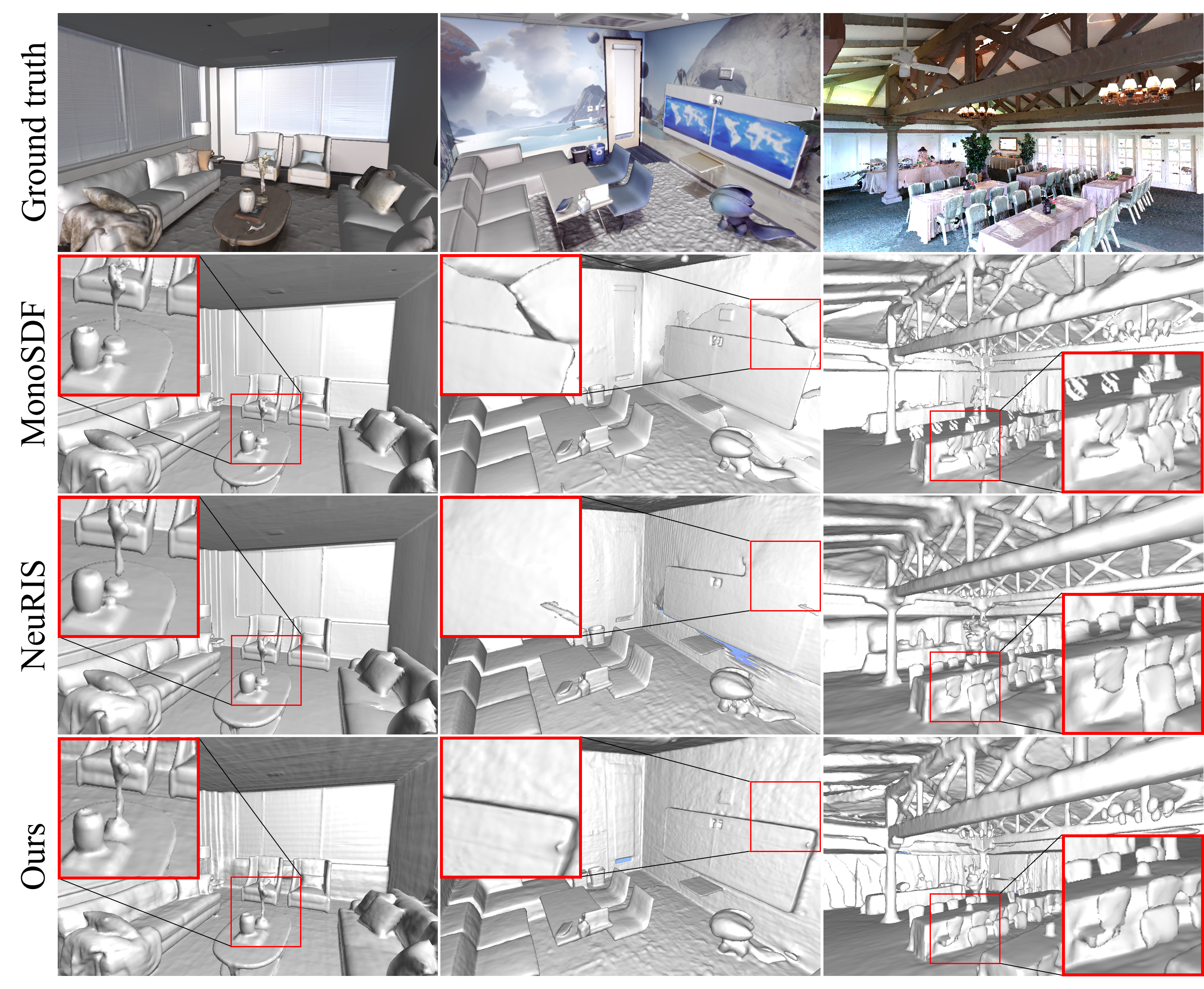
Figure 4: Qualitative comparison between the reconstructed meshes of Replica scan1 and scan4 and of Tanks and Temples’ Meetingroom by MonoSDF, NeuRIS and our method. The ground truth is colorful to contextualize the scene, while reconstruction are colorless to better appreciate geometry details. The red boxes underline the more accurate reconstruction achieved by our approach.

		GT Poses									COLMAP Poses
	scan	1	2	3	4	5	6	7	8	Mean	1	2	3	4	5	6	7	8	Mean
Chamfer $\downarrow$	MonoSDF Grids	2.22	2.27	1.63	3.53	4.36	2.00	2.16	2.21	2.55	2.23	2.64	1.62	3.15	4.44	2.03	2.19	2.22	2.56
	MonoSDF MLP	2.26	2.03	1.81	3.97	5.00	2.10	2.27	2.32	2.72	2.35	1.88	1.80	3.99	5.10	2.25	2.26	2.37	2.75
	NeuRIS	2.48	2.46	1.74	2.39	4.05	2.11	3.51	1.98	2.59	2.83	2.15	1.73	3.23	5.48	2.05	3.07	1.95	2.81
	MP-SDF (Ours)	2.60	1.75	1.74	1.58	2.14	2.32	2.80	2.30	2.15	3.00	1.64	1.80	2.12	2.60	2.19	2.94	2.20	2.31
F-score $\uparrow$	MonoSDF Grids	94.95	92.67	99.05	86.52	77.16	94.45	93.74	94.05	91.57	94.87	92.95	99.16	86.49	76.60	95.02	95.54	93.75	91.80
	MonoSDF MLP	95.36	96.20	98.72	84.94	72.29	95.03	95.75	93.75	91.51	93.34	96.98	97.99	83.82	71.54	92.07	95.83	92.82	90.55
	NeuRIS	92.83	95.10	97.75	91.48	75.23	94.76	90.88	97.69	91.97	88.56	95.70	97.99	86.22	66.42	94.87	88.95	97.93	89.58
	MP-SDF (Ours)	91.71	96.35	97.26	97.47	92.34	95.17	90.49	91.78	94.41	89.70	98.10	96.31	92.69	88.08	94.53	90.17	94.23	93.44

Table 1: Quantitative comparison of the accuracy on Replica dataset.

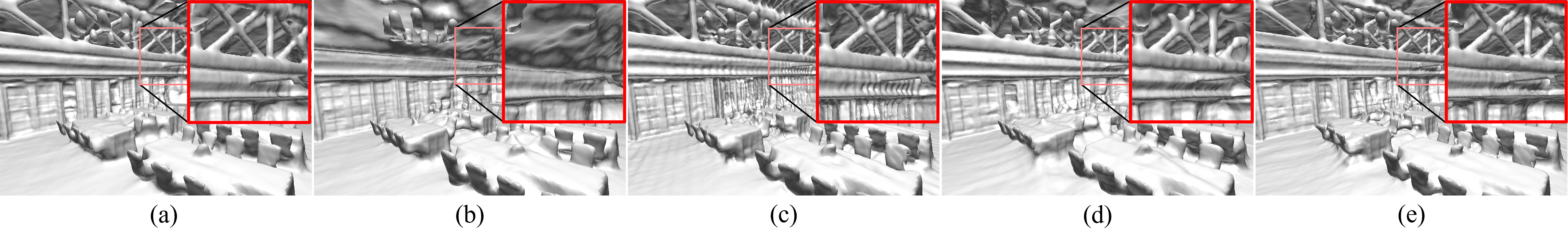
Figure 5: Ablation study results on Meetingroom. (a): full model, (b): w\o point cloud, (c): w\o depth map, (d): w\o exposure correction, (e): w\o normal regularization.

We implement our method on top of NeuS [Wang et al.(2021)Wang, Liu, Liu, Theobalt, Komura, and Wang]. The SDF function $f$ and the color $c$ are estimated by a MLP with 12 and 8 hidden layers, respectively. The SDF MLP is initialized to predict a sphere [Atzmon and Lipman(2020)]. The network input dimensionality is augmented by the positional encoding [Mildenhall et al.(2020)Mildenhall, Srinivasan, Tancik, Barron, Ramamoorthi, and Ng] with 10 and 4 frequencies for the 3D coordinates and the viewing direction, respectively. The model is trained for 300k iterations on an Nvidia A6000 using the Adam optimizer. The learning rate warmup proposed in NeuS [Wang et al.(2021)Wang, Liu, Liu, Theobalt, Komura, and Wang] is maintained. The warmup training stage consists of 60k iterations while the refinement stage covers the remaining iterations. In both stages, $1008$ rays are cast and $256$ points are sampled with the NeuS coarse-to-fine procedure, while 128 points are re-sampled by the soft depth supervision. The number of rays cast through the point cloud depends on the valid keypoints, while the maximum number of these rays is set to 128. The patch size and dilation rate for normal regularization are set to 3$\times$3 and $2$, respectively. The bilateral weights are computed by setting $\sigma_{c}=3$ and $\sigma_{d}=0.03$. In the sparse point cloud supervision, keypoints seen by less than 5 cameras are discarded. The loss weights are empirically set to $\lambda_{1}=\lambda_{3}=0.1$ while $\lambda_{2}$ starts at $0.5$ and decreases exponentially during the training, thus the point cloud can help at the beginning to initialize the model correctly, while in further stages the model can differentiate more from the initial prior.

4.2 3D Reconstruction Experiments

We compare our results against MonoSDF [Yu et al.(2022)Yu, Peng, Niemeyer, Sattler, and Geiger], the current state-of-the-art NeRF-based method for indoor geometry reconstruction, and against NeuRIS [Wang et al.(2022b)Wang, Wang, Long, Theobalt, Komura, Liu, and Wang], an improvement of NeuS exploiting normal maps for indoor reconstruction. MonoSDF relies on monocular depth and normal priors, while NeuRIS exploits monocular normal maps only, with a patch-match strategy to discard inaccurate normal priors. To provide geometric priors to these methods we employ Omnidata [Eftekhar et al.(2021)Eftekhar, Sax, Malik, and Zamir, Kar et al.(2022)Kar, Yeo, Atanov, and Zamir], as suggested by MonoSDF authors.

We test the methods starting from both images with ground truth and estimated poses: the results on the Replica dataset are shown in Tab. 1. On average, our model achieves better results in both cases and according to both metrics. With ground truth poses, the average F-score is $94.41$ against $91.97$ of the best competitor. Using COLMAP poses, results are similar: $93.44$ against $91.80$. The Chamfer distances also confirm these results. More in detail, for some scenes MP-SDF produces better reconstructions, while for the others the results are close to competitors. Looking at Fig. 4, it is clear how MonoSDF and NeuRIS produce good results in some environments but fail in some others, while our approach exhibits more stable results across all scenes. As an example, on Replica scan4, the wall behind the whiteboard presents some artefacts when reconstructed by concurrent methods, while MP-SDF reconstructs it correctly. This happens because the competitors rely heavily on input data from external monocular estimators that cannot offer strong reliability: these data may be inconsistent between subsequent frames and they may fail in case of prospectively misleading backgrounds, such as the painted wall in the second row. In our case, the depth maps are estimated by IterMVS, which is a MVS method, thus ensuring consistency over different images. See the supplementary material for more details.

Moreover, notice how the Omnidata model used by competitor methods to extract monocular clues was pre-trained on a poll of datasets, including Replica itself. To ensure fairness, the tests should be done on scenes not included in the Omnidata training. Therefore, we perform an additional test on the Meetingroom scene of the Tanks and Temples dataset. The results achieved by our model outperform the reconstructions of the other two methods, achieving a F-score of $52.53$ and a Chamfer distance of $10.02$. MonoSDF achieves F-score and Chamfer distance of $45.03$ and $11.22$, respectively, when trained with the multi-resolution grids and $40.45$ and $13.77$ with the MLP training. NeuRIS reaches a F-score of $37.13$ and a Chamfer distance of $12.32$. The fact that our method can outperform competitors even with a more “fair” training procedure is another proof of its value.

4.3 Ablation Study

We propose an ablation study on the employed supervision strategies to investigate the relevance of every contribution on the reconstruction quality. For this purpose, we show the results achieved by our ablated model on the scan1 and Meetingroom scenes.

		Scan1	Meetingroom
F-score $\uparrow$	MP-SDF (full model)	94.40	52.53
	w\o point cloud	93.14	39.25
	w\o depth map	90.18	47.90
	w\o exposure correction	94.20	39.36
	w\o normal regularization	92.55	46.63

Table 2: Ablation studies.

The results are presented in Tab. 2 and in Fig. 5.

All the supervision strategies contribute to improve the reconstruction quality. The two depth supervisions are effective in improving the geometry accuracy: without the point cloud supervision the reconstructed geometry is severely affected by a lack of guidance, leading to estimate wrong structures. On the other hand, the soft depth map supervision helps in removing periodic artifacts on surfaces, introducing a smoothing effect. The normal self-regularization permits to obtain a general smoothing of the surfaces, removing bumps but preserving the edge sharpness. The tests on the model with the exposure correction disabled show that it generally improves the reconstruction. This is more relevant in the Meetingroom scene, since it was acquired with variable exposure settings. On Replica scan1, acquired with fixed exposition and white balance, the exposure compensation effects are less relevant.

5 Limitations

State-of-the-art competitors like MonoSDF and NeuRIS compute losses from a direct comparison with the depth and/or normal maps generated with a monocular estimator. Thus, if these prior maps are very accurate, they produce good reconstructions. Differently, in MP-SDF the direct depth loss of the point cloud supervision affects only some pixels due to the point cloud sparsity, resulting in a softer guidance. Furthermore, MP-SDF depth soft supervision helps to focus the sampling but it does not enforce a direct constraint on the geometry. Similarly, MP-SDF normal regularization smooths artifacts out, but it does not directly force normal orientation. For these reasons, if the monocular priors are very accurate, our model could be outperformed by competitors. Generally, the monocular estimators produce very smooth maps, leading to reconstruct also smoother mesh with respect to our method which does not rely on monocular priors. Anyway, when monocular maps contain errors their reconstruction is strongly affected, as shown in Fig. 4.

6 Conclusion

In this work we introduce a novel approach targeting the reconstruction of complex indoor scenes. The joint usage of multiple priors, including soft depth supervision and advanced normal regularization strategies permits to achieve state-of-the-art results in 3D reconstruction. Future research will be devoted to the employment of multi-resolution schemes and to the reduction of the computational requirements.

Acknowledgment

This collaborative work was funded by Sony Europe B.V.. Special thanks go to Oliver Erdler, Yalcin Incesu and Piergiorgio Sartor for their support.

Supplementary Material

In this document we provide some additional details in order to better evaluate the performances of MP-SDF. Firstly, we present in detail the employed comparison metrics (Section A). Then, a further analysis is shown to justify the use of a MVS method rather than a monocular one for depth priors (Section B). Moreover, we discuss the exposure compensation effectiveness showing the results achieved on scenes acquired with variable or fixed exposure settings and then reconstructed with or without exposure compensation enabled (Section C). Finally, we present more qualitative results showing the reconstructed scenes (Section D).

Appendix A Quantitative Metrics

In this section, we recall the definition of the quantitative metrics employed in this work. In particular, we used the F-score and the Chamfer-L₁ distance. These two metrics compare the ground truth point cloud against the predicted one, extracted considering the set of vertexes of the respective mesh. The predicted mesh is produced by MP-SDF querying the SDF network on a three dimensional grid defined at a chosen resolution, then running the marching cubes algorithm [Lorensen and Cline(1987)]. In our experiments, aligned to what done in MonoSDF, the meshes are extracted from a grid at a resolution of $512\times 512\times 512$.

F-score

To define F-score, it is helpful to introduce precision $p$ and recall $r$ first. Precision is defined as follows:

$$p=\frac{1}{\left|\mathcal{P}\right|}\sum_{\mathbf{p}\in\mathcal{P}}\mathbf{1}_{T}\left(\,\text{min}_{\mathbf{p^{*}}\in\mathcal{P}^{*}}\lVert\mathbf{p}-\mathbf{p^{*}}\rVert\,\right)\quad\text{with}\quad\mathbf{1}_{T}(x):=\begin{cases}1\,\,\text{if}\,\,x\,<\,T\\ 0\,\,\text{if}\,\,x\,\geq\,T\end{cases}\vspace{-0.2cm}$$ (12)

where $\mathcal{P}$ is the predicted point cloud, $\mathcal{P}^{*}$ the ground truth one and $T=0.05$. Recall is defined as follows:

$$r=\frac{1}{\left|\mathcal{P}^{*}\right|}\sum_{\mathbf{p^{*}}\in\mathcal{P}^{*}}\mathbf{1}_{T}\left(\,\text{min}_{\mathbf{p}\in\mathcal{P}}\lVert\mathbf{p}-\mathbf{p^{*}}\rVert\,\right).$$ (13)

At this point, it is possible to define the F-score as follows:

$$\text{F-score}=\frac{2\cdot p\cdot r}{p+r}.$$ (14)

The F-score values presented in the main article are multiplied by a factor 100, to express them as percentages.

Chamfer-L₁ distance

To define the Chamfer-L₁ distance it is convenient to introduce the accuracy $a$ and the completeness $c$ first. The accuracy is defined as follows:

$$a=\frac{1}{\left|\mathcal{P}\right|}\sum_{\mathbf{p}\in\mathcal{P}}\left(\,\text{min}_{\mathbf{p^{*}}\in\mathcal{P}^{*}}\lVert\mathbf{p}-\mathbf{p^{*}}\rVert\,\right)$$ (15)

where $\mathcal{P}$ is the predicted point cloud and $\mathcal{P}^{*}$ the ground truth one. The completeness is defined as follows:

$$c=\frac{1}{\left|\mathcal{P}^{*}\right|}\sum_{\mathbf{p^{*}}\in\mathcal{P}^{*}}\left(\,\text{min}_{\mathbf{p}\in\mathcal{P}}\lVert\mathbf{p}-\mathbf{p^{*}}\rVert\,\right).$$ (16)

At this point, it is possible to define the Chamfer-L₁ distance as:

$$\text{Chamfer-{L}${}_{1}$}=\frac{a+c}{2}.$$ (17)

The F-score assigns a fixed weight to points with a distance larger than the selected threshold, independently on the actual error. On the contrary, the Chamfer-L₁ distance is computed considering every distance value, which makes it more sensible to outliers.

Appendix B Depth Prior Evaluation

In this section we propose a further investigation on the use of external priors. MonoSDF [Yu et al.(2022)Yu, Peng, Niemeyer, Sattler, and Geiger] and NeuRIS [Wang et al.(2022b)Wang, Wang, Long, Theobalt, Komura, Liu, and Wang] exploit monocular depth and normal maps produced by Omnidata [Eftekhar et al.(2021)Eftekhar, Sax, Malik, and Zamir] to supervise the training. Instead, MP-SDF exploits multi-view stereo depth maps obtained from IterMVS [Wang et al.(2022a)Wang, Galliani, Vogel, and Pollefeys].

We argue that geometric monocular cues can lead to wrong reconstructions: monocular approaches often produce predictions at a wrong scale and not consistent over subsequent frames. Moreover, in presence of flat but perspective coherent backgrounds, they may fail considering the 2D surface as part of the 3D volume. In the case of Replica scan4, presented in Fig. 6, the office wall is painted with a natural background. The monocular depth and normal estimations predict a depth and a normal maps that include geometric details of the background, even if the real surface is flat. Therefore, the reconstructed mesh is biased by these priors and exhibits artifacts on the wall. Considering Replica scan5 in Fig. 8, it is clear how Omnidata predicts wrong normals for the office walls. This strongly affects the reconstruction producing wall deformations.

Considering the same scenes reconstructed by MP-SDF supervised by IterMVS, it is possible to observe in Fig. 7 and Fig. 9 that they do not exhibit the artifacts mentioned above. Indeed, the MVS depth maps are more reliable and consistent with the real geometry of the scene. In particular, in scan4 the painting does not affect the depth estimation, which is consistent with the planar wall. Finally, in both the considered scenes, the IterMVS confidence maps show high reliability, thus enforcing the quality of MVS predictions.

Appendix C Exposure compensation effectiveness

In Fig. 10 we show the effect produced by the exposure compensation. In the first row, it is possible to see some of the input RGB images of the two datasets: the Replica Scan 1 is acquired with fixed exposure while the Tanks and Temples Meetingroom is captured with variable exposure. In the second and third rows, the normal maps of the reconstructions obtained with and without the exposure compensation are shown, respectively, while in the fourth row the difference map between normals is presented. As expected, its contribution on Replica is small, since input images were rendered with fixed exposure. Instead, it is very relevant on the Tanks and Temples scene, as it was acquired with variable exposure settings. The exposure compensation helps in reconstructing more accurately the structures on the ceiling and the challenging table and chair area in the middle of the room. As confirmed in Tab. 2 of the paper, the results achieved by the model without the exposure compensation are severely affected on the Tanks and Temples Meetingroom, while on Replica Scan 1 the ablation has almost no effect.

Appendix D Qualitative results

Fig. 11 presents some qualitative comparisons between MonoSDF [Yu et al.(2022)Yu, Peng, Niemeyer, Sattler, and Geiger], NeuRIS [Wang et al.(2022b)Wang, Wang, Long, Theobalt, Komura, Liu, and Wang] and our approach (MP-SDF) on the Replica dataset [Straub et al.(2019)Straub, Whelan, Ma, Chen, Wijmans, Green, Engel, Mur-Artal, Ren, Verma, Clarkson, Yan, Budge, Yan, Pan, Yon, Zou, Leon, Carter, Briales, Gillingham, Mueggler, Pesqueira, Savva, Batra, Strasdat, Nardi, Goesele, Lovegrove, and Newcombe] and on the Meetingroom scene from Tanks and Temples [Knapitsch et al.(2017)Knapitsch, Park, Zhou, and Koltun]. As discussed in the main article, on Replica our method outperforms the current state-of-the-art methods for indoor reconstruction, namely MonoSDF and NeuRIS. Differently from them, the visual quality of the reconstruction provided by MP-SDF is consistent across the different scenes in the figure, as also suggested by the quantitative results presented in the article. Finally, MP-SDF clearly outperforms the other methods also on Tanks and Temples Meetingroom in terms of visual quality, also in this case accordingly to the quantitative evaluation in the main article.

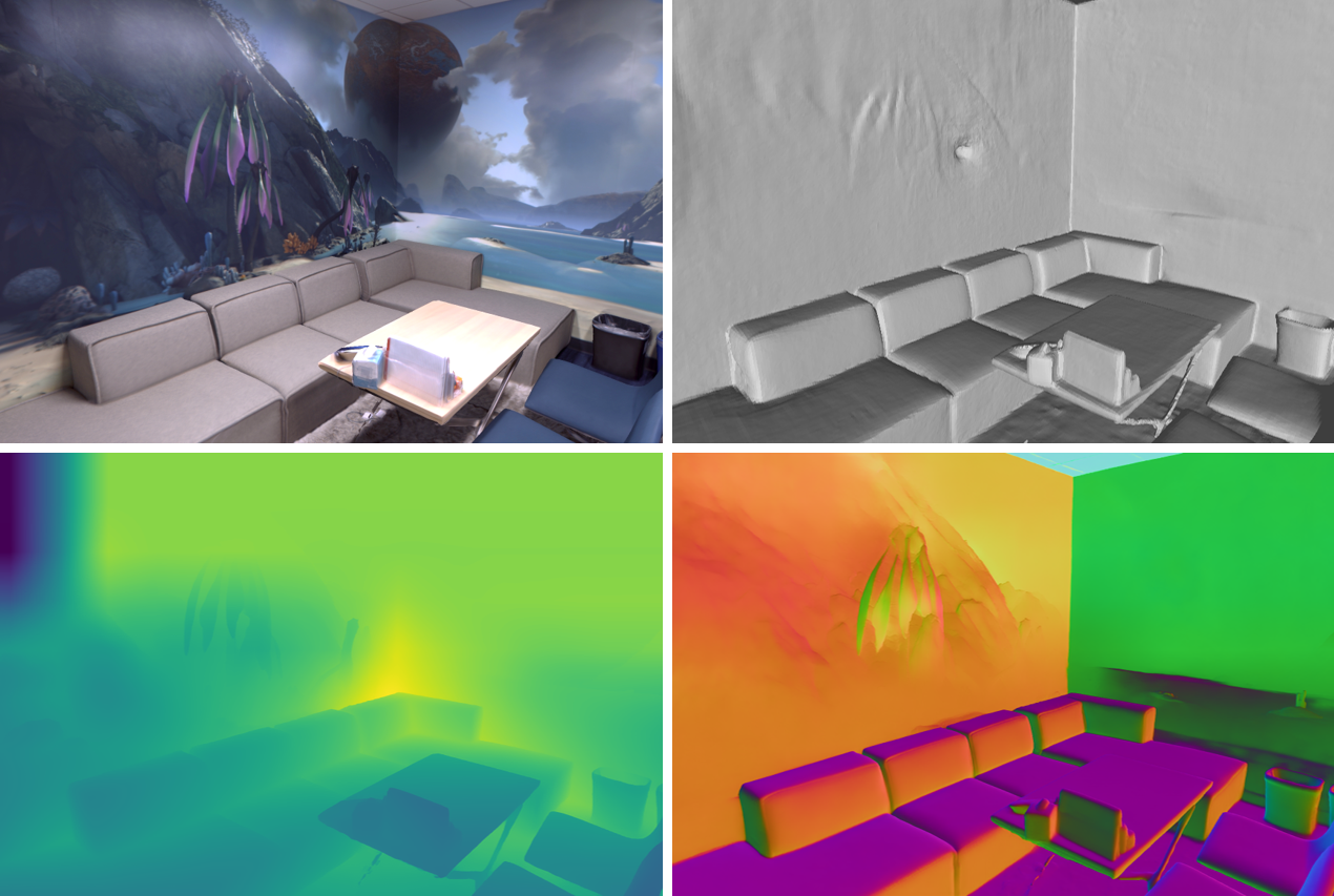
Figure 6: Replica scan4. From left to right and from top to bottom: RGB ground truth, MonoSDF reconstructed mesh, Omnidata depth map, Omnidata normal map.

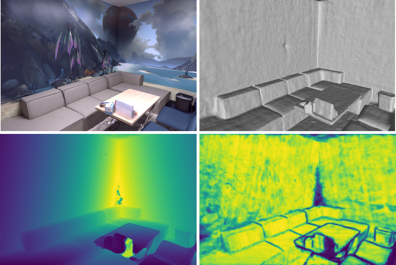
Figure 7: Replica scan4. From left to right and from top to bottom: RGB ground truth, MP-SDF (Ours) reconstructed mesh, IterMVS depth map, IterMVS confidence map.

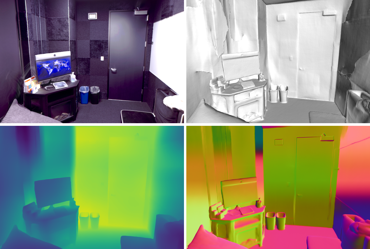
Figure 8: Replica scan5. From left to right and from top to bottom: RGB ground truth, MonoSDF reconstructed mesh, Omnidata depth map, Omnidata normal map.

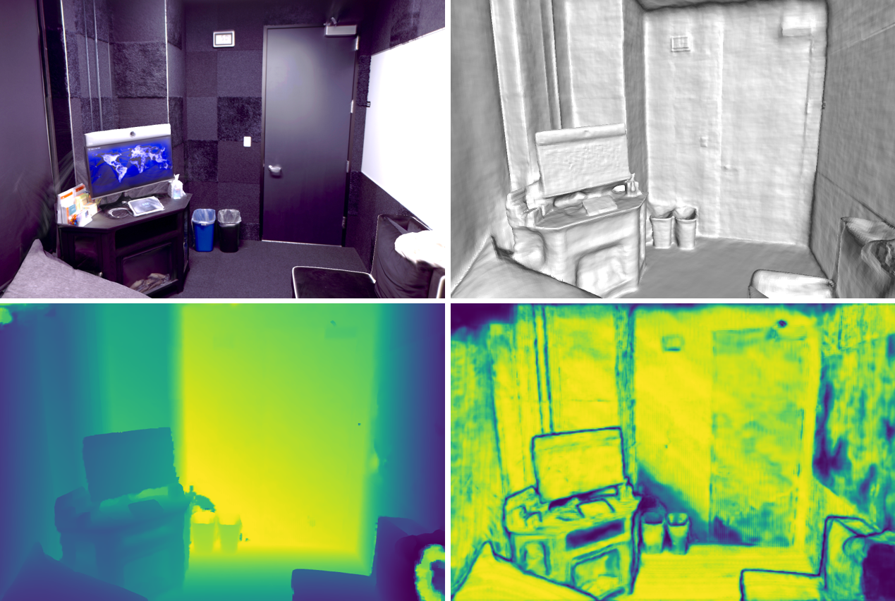
Figure 9: Replica scan5. From left to right and from top to bottom: RGB ground truth, MP-SDF (Ours) reconstructed mesh, IterMVS depth map, IterMVS confidence map.

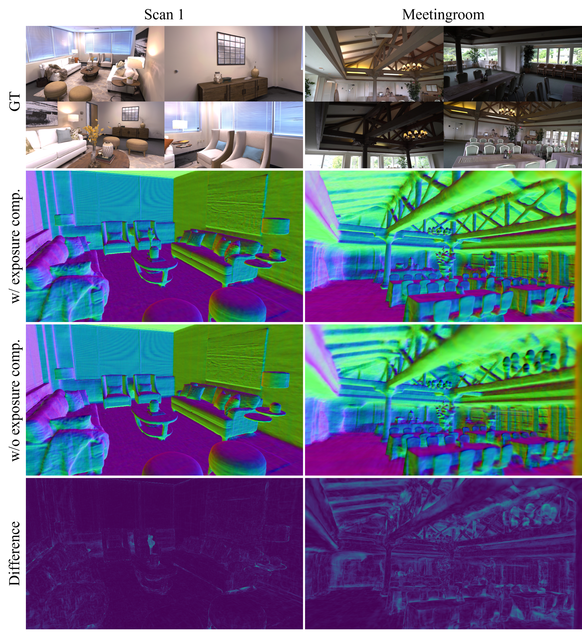
Figure 10: Exposure compensation effectiveness.

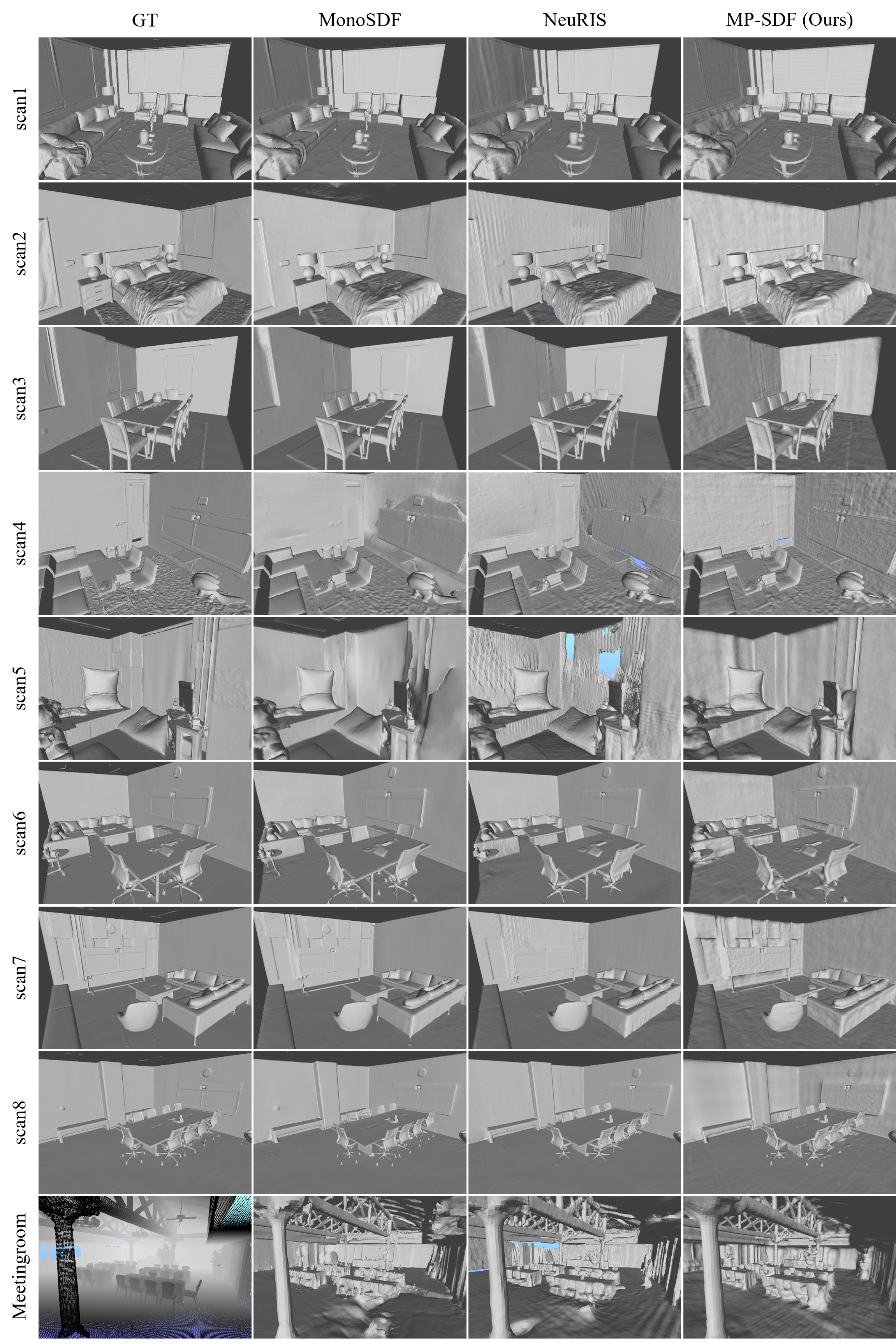
Figure 11: Qualitative evaluation on Replica and Tanks and Temples Meetingroom.

References

- [Achlioptas et al.(2018)Achlioptas, Diamanti, Mitliagkas, and Guibas] Panos Achlioptas, Olga Diamanti, Ioannis Mitliagkas, and Leonidas Guibas. Learning representations and generative models for 3d point clouds. In Proceedings of the International Conference on Machine Learning, pages 40–49. PMLR, 2018.
- [Atzmon and Lipman(2020)] Matan Atzmon and Yaron Lipman. Sal: Sign agnostic learning of shapes from raw data. In Proceedings of the IEEE Conference on Computer Vision and Pattern Recognition, June 2020.
- [Azinović et al.(2022)Azinović, Martin-Brualla, Goldman, Nießner, and Thies] Dejan Azinović, Ricardo Martin-Brualla, Dan B Goldman, Matthias Nießner, and Justus Thies. Neural rgb-d surface reconstruction. In Proceedings of the IEEE Conference on Computer Vision and Pattern Recognition, pages 6290–6301, June 2022.
- [Camuffo et al.(2022)Camuffo, Mari, and Milani] Elena Camuffo, Daniele Mari, and Simone Milani. Recent advancements in learning algorithms for point clouds: An updated overview. Sensors, 22(4):1357, 2022.
- [Chen et al.(2022)Chen, Xu, Geiger, Yu, and Su] Anpei Chen, Zexiang Xu, Andreas Geiger, Jingyi Yu, and Hao Su. Tensorf: Tensorial radiance fields. In Proceedings of the European Conference on Computer Vision, pages 333–350. Springer, 2022.
- [Chen et al.(2023)Chen, Xu, Wei, Tang, Su, and Geiger] Anpei Chen, Zexiang Xu, Xinyue Wei, Siyu Tang, Hao Su, and Andreas Geiger. Factor fields: A unified framework for neural fields and beyond. arXiv preprint arXiv:2302.01226, 2023.
- [Chen and Zhang(2019)] Zhiqin Chen and Hao Zhang. Learning implicit fields for generative shape modeling. In Proceedings of the IEEE Conference on Computer Vision and Pattern Recognition, pages 5939–5948, 2019.
- [Deng et al.(2022)Deng, Liu, Zhu, and Ramanan] Kangle Deng, Andrew Liu, Jun-Yan Zhu, and Deva Ramanan. Depth-supervised NeRF: Fewer views and faster training for free. In Proceedings of the IEEE Conference on Computer Vision and Pattern Recognition, June 2022.
- [Dupont et al.(2021)Dupont, Goliński, Alizadeh, Teh, and Doucet] Emilien Dupont, Adam Goliński, Milad Alizadeh, Yee Whye Teh, and Arnaud Doucet. Coin: Compression with implicit neural representations. In Proceedings of ICLR Workshop on Neural Compression: From Information Theory to Applications, 2021.
- [Eftekhar et al.(2021)Eftekhar, Sax, Malik, and Zamir] Ainaz Eftekhar, Alexander Sax, Jitendra Malik, and Amir Zamir. Omnidata: A scalable pipeline for making multi-task mid-level vision datasets from 3d scans. In Proceedings of the International Conference on Computer Vision, pages 10786–10796, 2021.
- [Fu et al.(2022)Fu, Xu, Ong, and Tao] Qiancheng Fu, Qingshan Xu, Yew-Soon Ong, and Wenbing Tao. Geo-neus: Geometry-consistent neural implicit surfaces learning for multi-view reconstruction. Advances in Neural Information Processing Systems, 2022.
- [Gadelha et al.(2017)Gadelha, Maji, and Wang] Matheus Gadelha, Subhransu Maji, and Rui Wang. 3d shape induction from 2d views of multiple objects. In Proceedings of the International Conference on 3D Vision, pages 402–411. IEEE, 2017.
- [Jimenez Rezende et al.(2016)Jimenez Rezende, Eslami, Mohamed, Battaglia, Jaderberg, and Heess] Danilo Jimenez Rezende, SM Eslami, Shakir Mohamed, Peter Battaglia, Max Jaderberg, and Nicolas Heess. Unsupervised learning of 3d structure from images. Advances in Neural Information Processing Systems, 29, 2016.
- [Kar et al.(2022)Kar, Yeo, Atanov, and Zamir] Oğuzhan Fatih Kar, Teresa Yeo, Andrei Atanov, and Amir Zamir. 3d common corruptions and data augmentation. In Proceedings of the IEEE Conference on Computer Vision and Pattern Recognition, pages 18963–18974, 2022.
- [Kato et al.(2018)Kato, Ushiku, and Harada] Hiroharu Kato, Yoshitaka Ushiku, and Tatsuya Harada. Neural 3d mesh renderer. In Proceedings of the IEEE Conference on Computer Vision and Pattern Recognition, pages 3907–3916, 2018.
- [Knapitsch et al.(2017)Knapitsch, Park, Zhou, and Koltun] Arno Knapitsch, Jaesik Park, Qian-Yi Zhou, and Vladlen Koltun. Tanks and temples: Benchmarking large-scale scene reconstruction. ACM Transactions on Graphics, 36(4), 2017.
- [Lorensen and Cline(1987)] William E Lorensen and Harvey E Cline. Marching cubes: A high resolution 3d surface construction algorithm. Proceedings of the ACM International Conference on Computer Graphics and Interactive Techniques, 21(4):163–169, 1987.
- [Martin-Brualla et al.(2021)Martin-Brualla, Radwan, Sajjadi, Barron, Dosovitskiy, and Duckworth] Ricardo Martin-Brualla, Noha Radwan, Mehdi S. M. Sajjadi, Jonathan T. Barron, Alexey Dosovitskiy, and Daniel Duckworth. NeRF in the Wild: Neural Radiance Fields for Unconstrained Photo Collections. In Proceedings of the IEEE Conference on Computer Vision and Pattern Recognition, 2021.
- [Mescheder et al.(2019)Mescheder, Oechsle, Niemeyer, Nowozin, and Geiger] Lars Mescheder, Michael Oechsle, Michael Niemeyer, Sebastian Nowozin, and Andreas Geiger. Occupancy networks: Learning 3d reconstruction in function space. In Proceedings of the IEEE Conference on Computer Vision and Pattern Recognition, pages 4460–4470, 2019.
- [Michalkiewicz et al.(2019)Michalkiewicz, Pontes, Jack, Baktashmotlagh, and Eriksson] Mateusz Michalkiewicz, Jhony K Pontes, Dominic Jack, Mahsa Baktashmotlagh, and Anders Eriksson. Implicit surface representations as layers in neural networks. In Proceedings of the International Conference on Computer Vision, pages 4743–4752, 2019.
- [Mildenhall et al.(2020)Mildenhall, Srinivasan, Tancik, Barron, Ramamoorthi, and Ng] Ben Mildenhall, Pratul P. Srinivasan, Matthew Tancik, Jonathan T. Barron, Ravi Ramamoorthi, and Ren Ng. Nerf: Representing scenes as neural radiance fields for view synthesis. In Proceedings of the European Conference on Computer Vision, 2020.
- [Müller et al.(2022)Müller, Evans, Schied, and Keller] Thomas Müller, Alex Evans, Christoph Schied, and Alexander Keller. Instant neural graphics primitives with a multiresolution hash encoding. ACM Transactions on Graphics (ToG), 41(4):1–15, 2022.
- [Niemeyer et al.(2020)Niemeyer, Mescheder, Oechsle, and Geiger] Michael Niemeyer, Lars Mescheder, Michael Oechsle, and Andreas Geiger. Differentiable volumetric rendering: Learning implicit 3d representations without 3d supervision. In Proceedings of the IEEE Conference on Computer Vision and Pattern Recognition, 2020.
- [Oechsle et al.(2021)Oechsle, Peng, and Geiger] Michael Oechsle, Songyou Peng, and Andreas Geiger. Unisurf: Unifying neural implicit surfaces and radiance fields for multi-view reconstruction. In Proceedings of the International Conference on Computer Vision, pages 5589–5599, 2021.
- [Park et al.(2019)Park, Florence, Straub, Newcombe, and Lovegrove] Jeong Joon Park, Peter Florence, Julian Straub, Richard Newcombe, and Steven Lovegrove. Deepsdf: Learning continuous signed distance functions for shape representation. In Proceedings of the IEEE Conference on Computer Vision and Pattern Recognition, pages 165–174, 2019.
- [Peng et al.(2021)Peng, Zhang, Xu, Wang, Shuai, Bao, and Zhou] Sida Peng, Yuanqing Zhang, Yinghao Xu, Qianqian Wang, Qing Shuai, Hujun Bao, and Xiaowei Zhou. Neural body: Implicit neural representations with structured latent codes for novel view synthesis of dynamic humans. In Proceedings of the IEEE Conference on Computer Vision and Pattern Recognition, pages 9054–9063, 2021.
- [Rematas et al.(2022)Rematas, Liu, Srinivasan, Barron, Tagliasacchi, Funkhouser, and Ferrari] Konstantinos Rematas, Andrew Liu, Pratul P. Srinivasan, Jonathan T. Barron, Andrea Tagliasacchi, Tom Funkhouser, and Vittorio Ferrari. Urban radiance fields. Proceedings of the IEEE Conference on Computer Vision and Pattern Recognition, 2022.
- [Roessle et al.(2022)Roessle, Barron, Mildenhall, Srinivasan, and Nießner] Barbara Roessle, Jonathan T. Barron, Ben Mildenhall, Pratul P. Srinivasan, and Matthias Nießner. Dense depth priors for neural radiance fields from sparse input views. In Proceedings of the IEEE Conference on Computer Vision and Pattern Recognition, June 2022.
- [Rossi et al.(2020)Rossi, Gheche, Kuhn, and Frossard] Mattia Rossi, Mireille El Gheche, Andreas Kuhn, and Pascal Frossard. Joint graph-based depth refinement and normal estimation. In Proceedings of the IEEE Conference on Computer Vision and Pattern Recognition, pages 12154–12163, 2020.
- [Saragadam et al.(2022)Saragadam, Tan, Balakrishnan, Baraniuk, and Veeraraghavan] Vishwanath Saragadam, Jasper Tan, Guha Balakrishnan, Richard G Baraniuk, and Ashok Veeraraghavan. Miner: Multiscale implicit neural representation. In Proceedings of the European Conference on Computer Vision, pages 318–333. Springer, 2022.
- [Schönberger and Frahm(2016)] Johannes Lutz Schönberger and Jan-Michael Frahm. Structure-from-motion revisited. In Proceedings of the IEEE Conference on Computer Vision and Pattern Recognition, 2016.
- [Schönberger et al.(2016)Schönberger, Zheng, Pollefeys, and Frahm] Johannes Lutz Schönberger, Enliang Zheng, Marc Pollefeys, and Jan-Michael Frahm. Pixelwise view selection for unstructured multi-view stereo. In Proceedings of the European Conference on Computer Vision, 2016.
- [Sormann et al.(2021)Sormann, Rossi, Kuhn, and Fraundorfer] Christian Sormann, Mattia Rossi, Andreas Kuhn, and Friedrich Fraundorfer. Ib-mvs: An iterative algorithm for deep multi-view stereo based on binary decisions. In Proceedings of the British Machine Vision Conference, 2021.
- [Straub et al.(2019)Straub, Whelan, Ma, Chen, Wijmans, Green, Engel, Mur-Artal, Ren, Verma, Clarkson, Yan, Budge, Yan, Pan, Yon, Zou, Leon, Carter, Briales, Gillingham, Mueggler, Pesqueira, Savva, Batra, Strasdat, Nardi, Goesele, Lovegrove, and Newcombe] Julian Straub, Thomas Whelan, Lingni Ma, Yufan Chen, Erik Wijmans, Simon Green, Jakob J. Engel, Raul Mur-Artal, Carl Ren, Shobhit Verma, Anton Clarkson, Mingfei Yan, Brian Budge, Yajie Yan, Xiaqing Pan, June Yon, Yuyang Zou, Kimberly Leon, Nigel Carter, Jesus Briales, Tyler Gillingham, Elias Mueggler, Luis Pesqueira, Manolis Savva, Dhruv Batra, Hauke M. Strasdat, Renzo De Nardi, Michael Goesele, Steven Lovegrove, and Richard Newcombe. The Replica dataset: A digital replica of indoor spaces. arXiv preprint arXiv:1906.05797, 2019.
- [Strümpler et al.(2022)Strümpler, Postels, Yang, Gool, and Tombari] Yannick Strümpler, Janis Postels, Ren Yang, Luc Van Gool, and Federico Tombari. Implicit neural representations for image compression. In Proceedings of the European Conference on Computer Vision, pages 74–91. Springer, 2022.
- [Wang et al.(2022a)Wang, Galliani, Vogel, and Pollefeys] Fangjinhua Wang, Silvano Galliani, Christoph Vogel, and Marc Pollefeys. Itermvs: iterative probability estimation for efficient multi-view stereo. In Proceedings of the IEEE Conference on Computer Vision and Pattern Recognition, pages 8606–8615, 2022a.
- [Wang et al.(2022b)Wang, Wang, Long, Theobalt, Komura, Liu, and Wang] Jiepeng Wang, Peng Wang, Xiaoxiao Long, Christian Theobalt, Taku Komura, Lingjie Liu, and Wenping Wang. Neuris: Neural reconstruction of indoor scenes using normal priors. In Proceedings of the European Conference on Computer Vision, pages 139–155. Springer, 2022b.
- [Wang et al.(2018)Wang, Zhang, Li, Fu, Liu, and Jiang] Nanyang Wang, Yinda Zhang, Zhuwen Li, Yanwei Fu, Wei Liu, and Yu-Gang Jiang. Pixel2mesh: Generating 3d mesh models from single rgb images. In Proceedings of the European Conference on Computer Vision, pages 52–67, 2018.
- [Wang et al.(2021)Wang, Liu, Liu, Theobalt, Komura, and Wang] Peng Wang, Lingjie Liu, Yuan Liu, Christian Theobalt, Taku Komura, and Wenping Wang. Neus: Learning neural implicit surfaces by volume rendering for multi-view reconstruction. Advances in Neural Information Processing Systems, 34:27171–27183, 2021.
- [Wang et al.(2022c)Wang, Han, Habermann, Daniilidis, Theobalt, and Liu] Yiming Wang, Qin Han, Marc Habermann, Kostas Daniilidis, Christian Theobalt, and Lingjie Liu. Neus2: Fast learning of neural implicit surfaces for multi-view reconstruction. arXiv preprint arXiv:2212.05231, 2022c.
- [Xu et al.(2022)Xu, Xu, Philip, Bi, Shu, Sunkavalli, and Neumann] Qiangeng Xu, Zexiang Xu, Julien Philip, Sai Bi, Zhixin Shu, Kalyan Sunkavalli, and Ulrich Neumann. Point-nerf: Point-based neural radiance fields. In Proceedings of the IEEE Conference on Computer Vision and Pattern Recognition, pages 5438–5448, 2022.
- [Yariv et al.(2020)Yariv, Kasten, Moran, Galun, Atzmon, Ronen, and Lipman] Lior Yariv, Yoni Kasten, Dror Moran, Meirav Galun, Matan Atzmon, Basri Ronen, and Yaron Lipman. Multiview neural surface reconstruction by disentangling geometry and appearance. Advances in Neural Information Processing Systems, 33, 2020.
- [Yu et al.(2022)Yu, Peng, Niemeyer, Sattler, and Geiger] Zehao Yu, Songyou Peng, Michael Niemeyer, Torsten Sattler, and Andreas Geiger. Monosdf: Exploring monocular geometric cues for neural implicit surface reconstruction. Advances in Neural Information Processing Systems, 2022.
- [Yüce et al.(2022)Yüce, Ortiz-Jiménez, Besbinar, and Frossard] Gizem Yüce, Guillermo Ortiz-Jiménez, Beril Besbinar, and Pascal Frossard. A structured dictionary perspective on implicit neural representations. In Proceedings of the IEEE Conference on Computer Vision and Pattern Recognition, pages 19228–19238, 2022.
- [Zanuttigh et al.(2016)Zanuttigh, Marin, Dal Mutto, Dominio, Minto, and Cortelazzo] Pietro Zanuttigh, Giulio Marin, Carlo Dal Mutto, Fabio Dominio, Ludovico Minto, and Guido Maria Cortelazzo. Time-of-Flight and Structured Light Depth Cameras: Technology and Applications. Springer, 2016.
- [Zhang et al.(2021)Zhang, Yao, and Quan] Jingyang Zhang, Yao Yao, and Long Quan. Learning signed distance field for multi-view surface reconstruction. In Proceedings of the International Conference on Computer Vision, pages 6525–6534, 2021.