Adaptive KalmanNet: Data-Driven Kalman Filter with Fast Adaptation
Abstract
Combining the classical kf (kf) with a dnn (dnn) enables tracking in partially known ss (ss) models. A major limitation of current dnn-aided designs stems from the need to train them to filter data originating from a specific distribution and underlying ss model. Consequently, changes in the model parameters may require lengthy retraining. While the kf adapts through parameter tuning, the black-box nature of dnn makes identifying tunable components difficult. Hence, we propose aknet (aknet), a dnn-aided kf that can adapt to changes in the ss model without retraining. Inspired by recent advances in llm fine-tuning paradigms, aknet uses a compact hypernetwork to generate cm weights. Numerical evaluation shows that aknet provides consistent state estimation performance across a continuous range of noise distributions, even when trained using data from limited noise settings.
Index Terms— Model-based deep learning, adaptive kf.
1 Introduction
Estimating the hidden state of a dynamic system from noisy observations is crucial in a wide range of applications [1]. Traditional mb (mb) methods, such as the kf [2], leverage mathematical parametric representations in the form of ss models that describe the underlying dynamics. The reliance of the kf and its variants on knowledge of the ss model implies that they are inherently adaptive, in the sense that changes in the model parameters are naturally incorporated into its operation. However, they are also sensitive to mismatches in the ss model, and are most suitable for models with Gaussian noises [1, Ch. 10].
Over the recent years, dnn-based filters have emerged as dd (dd) alternatives to mb filters. Highly parameterized dnn can be trained e2e using massive datasets for filtering without relying on the ss model [3]. Alternatively, one can fuse principled statistical models with a dd process via mb dl [4, 5], where the flow of the kf is preserved based on some of the SS model parameters and augmented with compact dnn [6, 7, 8, 9]. While hybrid mb/dd designs offer greater flexibility than their counterparts and support adaptation through compact dnn [10] (trainable with smaller datasets) and unsupervised learning [11, 7], they lack the inherent adaptivity of mb designs via mere parameter tuning. Adjusting a dd system to distribution shifts typically involves time-consuming and computationally intensive retraining [12].
In this work, we introduce aknet, an adaptive mb/dd filter that is trained with data to cope with a model mismatch, and can rapidly adapt to changes in the ss model without retraining. Our aknet extends kn[6] by adapting its mapping based on a context information parameter coined sow (sow). This sow is used as an input to a hypernetwork[13, 14], which fine-tunes kn’s dnn to adapt to different contexts. When tracking in face of partially-known non-Gaussian ss models, the sow serves as an indicator for the variances of the noise signals.
Unlike previously proposed hypernetworks [15, 16, 17], aknet is tailored for a compact implementation, and it draws inspiration from recent cm (cm) techniques in llm — used for fine-tuning general llm to specialized tasks [18]. Our approach achieves a significant reduction in trainable parameters, outperforming both alternative hypernetworks [13] and ensemble (filter-bank) architectures [19]. To facilitate ”learning to filter” across different ss models, we propose a dedicated two-stage training method. In numerical evaluations, aknet consistently estimates states across a continuous range of unseen distributions with varied noise variances, even when trained on limited data from a discrete set of distributions. Furthermore, it successfully tracks rapidly changing distributions and shows robustness against errors in sow estimation.
2 PROBLEM FORMULATION
2.1 State Estimation
We consider dynamical systems characterized by a ss model in discrete-time. We focus on linear models with unknown time-varying noise signals, which (possibly) follow non-Gaussian distributions
| (1a) | ||||||
| (1b) | ||||||
Here, is the latent state vector at time , which is evolved by a state evolution matrix , and by an additive zero-mean process noise . The vector represents the observations at time , which is generated from the latent state by a linear mapping , and corrupted by an additive zero-mean noise .
2.2 Preliminaries
Given knowledge of and , kf is mse optimal if both follow Gaussian distributions. This is achieved by first predicting the next state and observations based on the previous estimate via
| (2) |
The next estimate is obtained using the observed as follows
| (3) |
where is the kg (kg) computed by tracking the second order moments, using and . For unknown and , a range of adaptive kf methods [20] have been proposed, with the main idea of adding a noise estimator on top of kf. These mb approaches manage noise shifts conveniently through tuning the parameters and that are fed into the kf.
The dnn-aided kn [6] is trained to produce state estimates in a discriminative manner [21]. It can successfully learn from data to cope with non-Gaussian distributions. This is achieved by preserving the operation of the kf in (2)-(3), while computing the kg using a dnn with parameters , comprised of a rnn (rnn) with preceding and subsequent fc (fc) layers, denoted , applied to features extracted from and .
2.3 Fast Adaptation Problem
dnn-aided filters such as kn can cope with non-Gaussian noises and possible mismatches in and ; however, they are typically trained for a specific ss model. The parameters of kn are trained using data corresponding to (at most) a limited set of distributions. In our time-varying setting, a typical kf implementation would involve an additional estimator for recovering and which can be substituted into its computation of . This ability is not supported by dnn-aided filters such as kn, even when one has access during run-time to instantaneous estimates of and . Thus, we wish to extend kn to reliably track in ss models with time-varying noise statistics.
In particular, we do not assume full knowledge of matrices and , but rather only to the scalar indicating the rough scaling ratio between process noise and observation noise, given by
| (4) |
This formulation of the sow is selected due to it being sufficient statistics for computing the kg in linear Gaussian ss models with scaled identity noise variance matrices [22]. We assume that the system has access to (4), possibly provided by some external estimator, noting that estimating this scalar quantity is expected to be notably simpler compared to estimating the matrices and .
The training dataset comprises length state trajectories alongside their corresponding sow, i.e.,
| (5) |
The sow in (5) may cover only a few discrete points of noise settings. During inference, the system is required to be able to track over a continuous range of noise settings.
3 Adaptive KalmanNet
3.1 Architecture
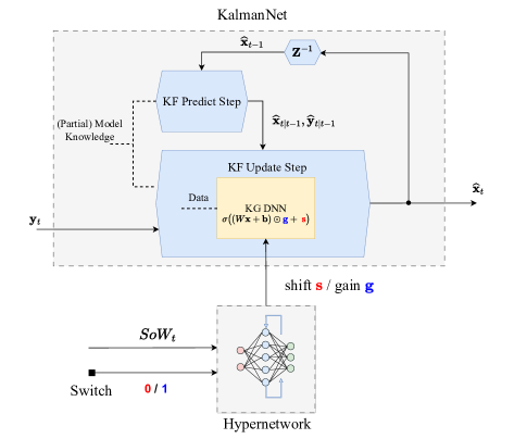
aknet is an extension of kn, designed to handle time-varying noise distributions. Given the context , a compact hypernetwork with parameters generates cm weights. These cm weights then fine-tune the kg dnn parameters, such that the kg computed by kn becomes .
Hypernetwork: In general, hypernetworks utilize additional dnn to generate the parameters of another dnn [13]. This allows the dnn mapping to be influenced by additional features. Hypernetworks are typically very highly parameterized, with many output neurons dictated by the number of dnn parameters, making them computationally expensive and challenging to train. To exploit the ability of hypernetworks to set the kg dnn mapping based on without dramatically increasing parameterization, we employ cm [18]. Instead of generating all the parameters of kg dnn, cm fine-tunes the original parameters. The hypernetwork with parameters induces a mapping with cm weights as output: gain and shift , whereas gain represents a multiplicative modulation and shift represents an additive modulation, respectively. To be parameter efficient, we reuse the same hypernetwork to generate and through an additional input , such that
| (6) |
cm: cm performs on the level of neuronal computation. It is applied in aknet to both fc layers and rnn layers of kn. To formulate the operation of cm, we consider a generic form of linear computation with weights and bias applied with a with nonlinear activation function , i.e., . This form describes both fc layers and the gate computations in rnn. With cm applied, the operation of such a layer becomes
| (7) |
where represents element-wise multiplication, and are the gains and shifts obtained from the neurons of the hypernetwork corresponding to the current layer via (6). The resulting architecture is illustrated in Fig. 1.
3.2 Training
The training of aknet is based on the loss, which for a dataset is given by (omitting weights regularization)
| (8) |
In (8), is the estimation of produced from by aknet with parameters .
We train aknet in two stages. We first train only kn. To that aim, we fix the cm layer not to affect the kg computation, i.e., to output unit gains and zero shift, and extract a subset where all trajectories have a relatively stationary and similar noise distributions. We then train solely based on the loss . In the second stage, we freeze , and train only the hypernetwork parameters . Here, we use the entire dataset , which encompasses non-stationary noise distributions, and train with the fixed based on .
3.3 Discussion
aknet allows dnn-aided tracking to be carried out in ss models with time-varying noise statistics without requiring retraining. It is based on kn due to its preservation of the majority of the mb attributes intrinsic to the kf. As kg effectively encodes the information regarding the noise statistics, aknet enables adaptation by augmenting it with a dedicated hypernetwork. It uses a hypernetwork based on cm due to its parameter efficiency and quick adaptation. The former is illustrated in Table 1, reporting the number of trainable parameters of aknet used for different ss model sizes. We observe in Table 1 that the number of cm weights is much smaller than that of kn, showcasing superior parameter efficiency over employing ensemble (filter-bank) designs. The trained hypernetwork, which maps into cm weights, facilitates fast adaptation in online inference. The overall approach addresses a frequent challenge in dd methods: the ambiguous task of determining which parameters require tuning for a specific shift. The rationale used in aknet can be extended to alternative hybrid mb/dd systems employed in time-varying conditions.
Our problem formulation considers the sow as being externally provided, while in practice, it should be estimated. There are various ways to estimate . This noise estimator design is mainly a tradeoff between robustness and inference speed. For example, em [23] algorithm is more robust since its convergence can be guaranteed, while correlation-based methods [24, 25] using one-step estimation can be much faster while less guaranteed in terms of performance. In our case, since is only a scalar, a simple estimation method is grid search with unsupervised loss as criteria. Alternatively, it can be based on a machine learning estimator that is jointly trained alongside the hypernetwork. In our numerical study in Section 4, we show that aknet is robust to errors in the sow, and leave its study with sow estimation for future work.
kn Hypernet [13] cm Ensemble 10k 6k 1k 22k 90k 1.5k 330k 100k 6k
4 Numerical Evaluations
In this section we provide a numerical evaluation of aknet. We consider three ss models with different noise distributions111The source code can be found online at https://github.com/KalmanNet/Adaptive-KNet-ICASSP24.: a Gaussian setting, showcasing the ability of aknet to achieve the optimal mse of the mb kf; a non-Gaussian setting, demonstrating aknet’s gains in coping with non-Gaussian noises; and a setting with noisy sow, studying the robustness of aknet to errors in this feature. Unless stated otherwise, we set and with , such that . The pseudo-stationary dataset used to train has 100 trajectories with noise setting , , while used to the train the hypernetwork has 400 trajectories.
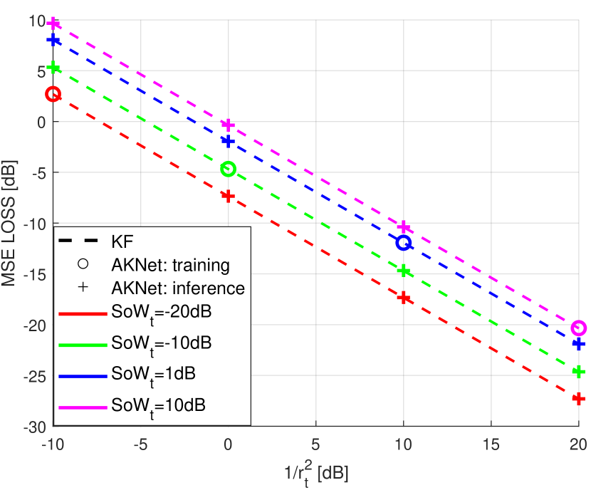
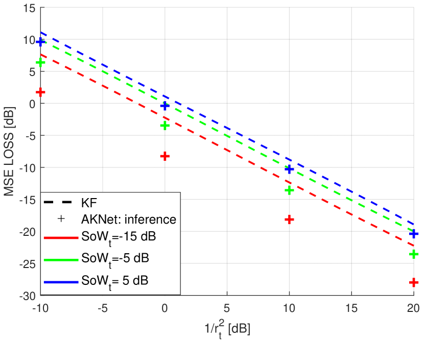
Gaussian Noise: First, we evaluate aknet on a linear Gaussian ss model. We randomly set and , only requiring them to be positive definite (no need to be diagonal). The data set contains only four different noise variance pairs. In Fig. 2, the dashed lines represent the performances of the kf on these datasets, serving as an optimal baseline given the linear Gaussian setting. The figure reveals that aknet not only coincides with the kf for the four sow observed during training, but also generalizes to unseen distributions. This generalization includes both ss models with the same ratio but with differing scaling values , as well as ss models with ratios that are unseen during training. This demonstrates that aknet only needs a small amount of training data on a limited number of settings in order for it to handle a wide varying range of noise statistics.
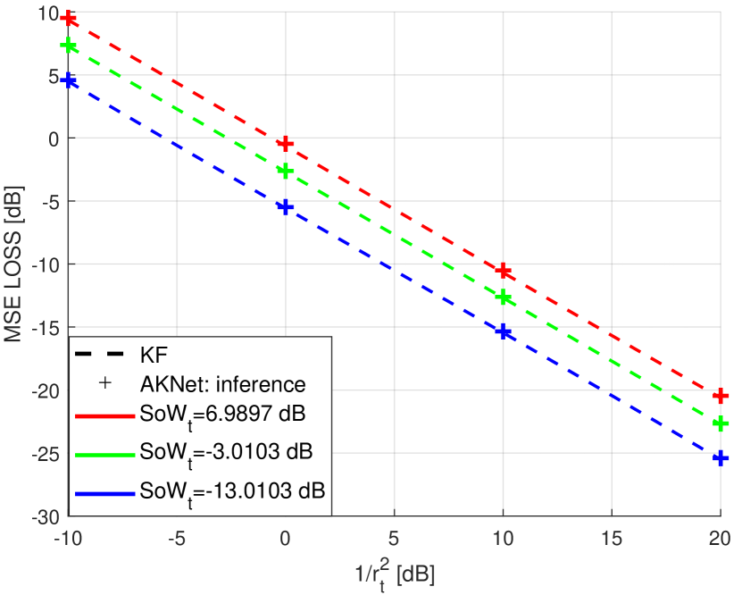
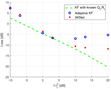
Non-Gaussian Noise: We use exponentially distributed noise signals that are spatially uncorrelated, i.e., and are scaled identity matrices. We again train aknet using merely four different distribution pairs, and test it on ss models with different distributions that either preserve sow observed in training as well as sow seen only in inference. The results, reported in Fig. 3, highlight that the two forms of generalization capabilities are still kept even for the non-Gaussian case. Furthermore, aknet can significantly outperform classic kf, due to the suitability of kn in handling non-Gaussian distributions.
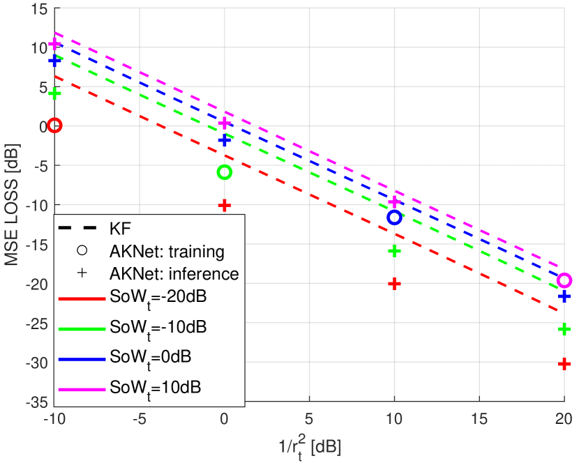
Noisy sow: So far, we have shown that aknet incorporates a continuous shifting range of noise distributions in its compact network model. We next study its ability to cope with noisy sow, arising from estimation errors encountered during online inference with time-varying noise distributions. We again consider a Gaussian ss model, and train aknet with the same data as that used in Fig. 2. During inference, the time-variations simulate abrupt jumps. Particularly, we assume that the scaling parameters jump to different values in each timestep . The simulation results shown in Fig. 4 are generated with ground truth scaling parameters at previous timestep and jump to . For fair comparison, aknet uses the same correlation-based noise estimator [25] as the adaptive kf.
In Fig. 4, both kf and aknet remain optimal when the jumping step of is not large. However, as the jumping step increases, especially in low observation noise scenarios, adaptive kf produces much worse state estimation than aknet. In summary, aknet can keep track of jumping noise distributions, approaching optimal state estimation provided the jumping step remains within a certain limit. If it is outside the limit, aknet can still do better than classic kf even in this linear Gaussian setting. The correlation-based noise estimator we choose values inference speed over accuracy, showing the robustness of aknet to noise estimation errors.
5 Conclusions
We have presented aknet, a dnn-aided kf capable of handling varying noise statistics using a single parameter tuning. aknet utilizes a compact hypernetwork to generate cm weights and employs a two-stage training process. Numerical evaluation shows aknet’s adaptability to varying noise distributions during state estimation and robustness in online tracking, with noise estimation errors. Although primarily tailored for state estimation, the fundamental principles could potentially be adapted for other DD signal processing systems in dynamic scenarios.
References
- [1] J. Durbin and S. J. Koopman, Time Series Analysis by State Space Methods. OUP Oxford, 2012, vol. 38.
- [2] R. E. Kalman, “A New Approach to Linear Filtering and Prediction Problems,” Journal of Basic Engineering, vol. 82, no. 1, pp. 35–45, 1960.
- [3] P. Becker, H. Pandya, G. Gebhardt, C. Zhao, C. J. Taylor, and G. Neumann, “Recurrent Kalman Networks: Factorized Inference in High-Dimensional Deep Feature Spaces,” in International Conference on Machine Learning. PMLR, 2019, pp. 544–552.
- [4] N. Shlezinger, J. Whang, Y. C. Eldar, and A. G. Dimakis, “Model-Based Deep Learning,” Proc. IEEE, vol. 111, no. 5, pp. 465–499, 2023.
- [5] N. Shlezinger and Y. C. Eldar, “Model-Based Deep Learning,” Foundations and Trends® in Signal Processing, vol. 17, no. 4, pp. 291–416, 2023.
- [6] G. Revach, N. Shlezinger, X. Ni, A. L. Escoriza, R. J. Van Sloun, and Y. C. Eldar, “KalmanNet: Neural Network Aided Kalman Filtering for Partially Known Dynamics,” IEEE Trans. Signal Process., vol. 70, pp. 1532–1547, 2022.
- [7] A. Ghosh, A. Honoré, and S. Chatterjee, “DANSE: Data-Driven Non-Linear State Estimation of Model-Free Process in Unsupervised Learning Setup,” arXiv preprint arXiv:2306.03897, 2023.
- [8] G. Choi, J. Park, N. Shlezinger, Y. C. Eldar, and N. Lee, “Split-KalmanNet: A Robust Model-Based Deep Learning Approach for State Estimation,” IEEE Trans. Veh. Technol., 2023.
- [9] G. Revach, X. Ni, N. Shlezinger, R. J. G. van Sloun, and Y. C. Eldar, “RTSNet: Learning to Smooth in Partially Known State-Space Models,” IEEE Trans. Signal Process., vol. 71, pp. 4441–4456, 2023.
- [10] G. Revach, N. Shlezinger, R. J. G. van Sloun, and Y. C. Eldar, “KalmanNet: Data-Driven Kalman Filtering,” in IEEE International Conference on Acoustics, Speech and Signal Processing (ICASSP), 2021, pp. 3905–3909.
- [11] G. Revach, N. Shlezinger, T. Locher, X. Ni, R. J. van Sloun, and Y. C. Eldar, “Unsupervised Learned Kalman Filtering,” in European Signal Processing Conference (EUSIPCO), 2022, pp. 1571–1575.
- [12] T. Raviv, S. Park, O. Simeone, Y. C. Eldar, and N. Shlezinger, “Adaptive and Flexible Model-Based AI for Deep Receivers in Dynamic Channels,” IEEE Wireless Communications Magazine, 2023.
- [13] D. Ha, A. Dai, and Q. V. Le, “Hypernetworks,” arXiv preprint arXiv:1609.09106, 2016.
- [14] T. Galanti and L. Wolf, “On the Modularity of Hypernetworks,” Advances in Neural Information Processing Systems, vol. 33, pp. 10 409–10 419, 2020.
- [15] M. Goutay, F. A. Aoudia, and J. Hoydis, “Deep Hypernetwork-Based MIMO Detection,” in Proc. IEEE SPAWC, 2020.
- [16] Y. Liu and O. Simeone, “Learning How to Transfer From Uplink to Downlink via Hyper-Recurrent Neural Network for FDD Massive MIMO,” IEEE Trans. Wireless Commun., vol. 21, no. 10, pp. 7975–7989, 2022.
- [17] K. Pratik, R. A. Amjad, A. Behboodi, J. B. Soriaga, and M. Welling, “Neural Augmentation of Kalman Filter with Hypernetwork for Channel Tracking,” in Proc. IEEE GLOBECOM, 2021.
- [18] N. Ding, Y. Qin, G. Yang, F. Wei, Z. Yang, Y. Su, S. Hu, Y. Chen, C.-M. Chan, W. Chen et al., “Parameter-Efficient Fine-Tuning of Large-Scale Pre-Trained Language Models,” Nature Machine Intelligence, pp. 1–16, 2023.
- [19] M. Khodarahmi and V. Maihami, “A Review on Kalman Filter Models,” Archives of Computational Methods in Engineering, vol. 30, no. 1, pp. 727–747, 2023.
- [20] L. Zhang, D. Sidoti, A. Bienkowski, K. R. Pattipati, Y. Bar-Shalom, and D. L. Kleinman, “On the Identification of Noise Covariances and Adaptive Kalman Filtering: A New Look at A 50 Year-Old Problem,” IEEE Access, vol. 8, pp. 59 362–59 388, 2020.
- [21] N. Shlezinger and T. Routtenberg, “Discriminative and Generative Learning for Linear Estimation of Random Signals [Lecture Notes],” IEEE Signal Process. Mag., vol. 40, no. 6, pp. 75–82, 2023.
- [22] S. Sangsuk-Iam and T. Bullock, “Analysis of Discrete-Time Kalman Filtering Under Incorrect Noise Covariances,” IEEE Trans. Autom. Control, vol. 35, no. 12, pp. 1304–1309, 1990.
- [23] J. Dauwels, S. Korl, and H.-A. Loeliger, “Expectation Maximization as Message Passing,” arXiv preprint cs/0508027, 2005.
- [24] R. Mehra, “On the Identification of Variances and Adaptive Kalman Filtering,” IEEE Trans. Autom. Control, vol. 15, no. 2, pp. 175–184, 1970.
- [25] S. Akhlaghi, N. Zhou, and Z. Huang, “Adaptive Adjustment of Noise Covariance in Kalman Filter for Dynamic State Estimation,” in IEEE Power & Energy Society General Meeting, 2017.