Stabilization of 2D Navier–Stokes equations by means of actuators with locally supported vorticity

Abstract.

Exponential stabilization to time-dependent trajectories for the incompressible Navier–Stokes equations is achieved with explicit feedback controls. The fluid is contained in two-dimensional spatial domains and the control force is, at each time instant, a linear combination of a finite number of given actuators. Each actuator has its vorticity supported in a small subdomain. The velocity field is subject to Lions boundary conditions. Simulations are presented showing the stabilizing performance of the proposed feedback. The results also apply to a class of observer design problems.

1. Introduction

Let us be given a trajectory $y_{\tt t}$ of the Navier–Stokes system as

$$\tfrac{\partial}{\partial t}y_{\tt t}-\nu\Delta y_{\tt t}+\langle y_{\tt t}\cdot\nabla\rangle y_{\tt t}+\nabla p_{\tt t}=f,\qquad\mathop{\rm div}\nolimits y_{\tt t}=0,$$ (1.1a)

$${\mathcal{G}}y_{\tt t}\left.\kern-2.4pt\right|_{\partial\Omega}=0,\qquad y_{\tt t}(0,\raisebox{-1.07639pt}{\scalebox{1.25}{$\cdot$}})=y_{{\tt t}0}.$$ (1.1b)

The spatial domain $\Omega\in{\mathbb{R}}^{2}$, is a bounded convex polygonal domain. Denoting by $(t,x)$ a generic point in the cylinder $(0,+\infty)\times\Omega$, the state $y_{\tt t}=y_{\tt t}(t,x)\in{\mathbb{R}}^{2}$ is the velocity vector,  $p_{\tt t}=p_{\tt t}(t,x)\in{\mathbb{R}}$ represents the pressure function, $f=f(t,x)\in{\mathbb{R}}^{2}$ is an given external body force, and $y_{{\tt t}0}=y_{{\tt t}0}(x)\in{\mathbb{R}}^{2}$ is a given initial velocity field, at time $t=0$. The divergence free relation

$$0=\mathop{\rm div}\nolimits y_{\tt t}\eqqcolon\tfrac{\partial}{\partial x_{1}}{y_{\tt t}}_{1}+\tfrac{\partial}{\partial x_{2}}{y_{\tt t}}_{2}$$

means that we consider incompressible fluids. Above, $({y_{\tt t}}_{1},{y_{\tt t}}_{2})\coloneqq y_{\tt t}$ and $(x_{1},x_{2})\coloneqq x$ denote the coordinates of the state $y_{\tt t}$ and of the spatial point $x\in\Omega$. The operators $\Delta$ and $\nabla$ stand for the usual Laplacian and gradient operators, formally, for a scalar function $g=g(x)$,

$$\Delta g\coloneqq(\tfrac{\partial}{\partial x_{1}})^{2}g+(\tfrac{\partial}{\partial x_{2}})^{2}g,\qquad\nabla g\coloneqq\left(\tfrac{\partial}{\partial x_{1}}g,\tfrac{\partial}{\partial x_{2}}g\right)$$

and for vector fields $y=(y_{1},y_{2})$ and $z=(z_{1},z_{2})$,

$$\Delta y=(\Delta y_{1},\Delta y_{2})\qquad\langle y\cdot\nabla\rangle z\coloneqq\left(y\cdot\nabla z_{1},y\cdot\nabla z_{2}\right).$$

Finally, the relation ${\mathcal{G}}y_{\tt t}\left.\kern-2.4pt\right|_{\partial\Omega}=0$ stands for the (homogeneous) boundary conditions of the fluid velocity $y_{\tt t}$. We shall assume Lions boundary conditions. Namely, firstly the velocity is tangent to the boundary, that is, $(y_{\tt t}\cdot{\mathbf{n}})\left.\kern-2.4pt\right|_{\partial\Omega}=0$ where ${\mathbf{n}}$ stands for the unit outward normal vector to the boundary $\partial\Omega$ of $\Omega$. We complement this with a condition for the vorticity function

$$w_{\tt t}\coloneqq\mathop{\rm curl}\nolimits y_{\tt t}\coloneqq\tfrac{\partial}{\partial x_{2}}{y_{\tt t}}_{1}-\tfrac{\partial}{\partial x_{1}}{y_{\tt t}}_{2}.$$ (1.2)

That is, Lions boundary conditions correspond to

$${\mathcal{G}}y_{\tt t}\coloneqq(y_{\tt t}\cdot{\mathbf{n}},\mathop{\rm curl}\nolimits y_{\tt t}).$$ (1.3)

The terminology is motivated by [21, Sect. 6.9] and is also adopted in [18, 23]. It distinguishes Lions boundary conditions as a subclass of the more general class of Navier (slip) boundary conditions [18, Cor. 4.3], which are appropriate to model the fluid velocity in some situations [14]; for further works addressing these conditions we refer to [15, 16, 12, 13, 2] and references therein.

1.1. Stabilization to trajectories.

In real world applications we will likely have at our disposal a finite number of actuators only. We take this into consideration throughout this manuscript by taking a finite number $M_{\sigma}$ of vector fields $\Phi_{j}=\Phi_{j}(x)$, $1\leq j\leq M_{\sigma}$, as actuators. Given a different initial state $y_{0}\neq{y_{\tt t0}}$ we want to find a control input $u=u(t)\in{\mathbb{R}}^{M_{\sigma}}$ such that the solution $y$ of the controlled Navier–Stokes system

$$\tfrac{\partial}{\partial t}y-\nu\Delta y+\langle y\cdot\nabla\rangle y+\nabla p=f+\sum_{j=1}^{M_{\sigma}}u_{j}\Phi_{j},\qquad\mathop{\rm div}\nolimits y=0,$$ (1.4a)

$${\mathcal{G}}y\left.\kern-2.4pt\right|_{\partial\Omega}=0,\qquad y(0,\raisebox{-1.07639pt}{\scalebox{1.25}{$\cdot$}})=y_{0}.$$ (1.4b)

converges to the targeted solution $y_{\tt t}$ as time increases. The scalars $u_{j}=u_{j}(t)$ stand for the coordinates of the input vector, $u\eqqcolon(u_{1},\dots,u_{M_{\sigma}})$, at time $t$.

Furthermore, we would like that $y(t,\raisebox{-1.07639pt}{\scalebox{1.25}{$\cdot$}})$ converges to $y_{\tt t}(t,\raisebox{-1.07639pt}{\scalebox{1.25}{$\cdot$}})$ exponentially with an arbitrary apriori given rate $\mu>0$. Finally, we look for an input in feedback form as

$$u(t)={\mathbf{K}}(t,y(t,\raisebox{-1.07639pt}{\scalebox{1.25}{$\cdot$}})-y_{\tt t}(t,\raisebox{-1.07639pt}{\scalebox{1.25}{$\cdot$}}))\in{\mathbb{R}}^{M_{\sigma}},\qquad\mbox{shortly }u={\mathbf{K}}(y-y_{\tt t}),$$

depending only on time $t$ and on the difference between the current controlled state $y(t,\raisebox{-1.07639pt}{\scalebox{1.25}{$\cdot$}})$ and the targeted state $y_{\tt t}(t,\raisebox{-1.07639pt}{\scalebox{1.25}{$\cdot$}})$ at time $t$.

Let us denote by $U_{M}$ the linearly independent set of actuators,

$$U_{M}\coloneqq\{\Phi_{i}^{M}\mid 1\leq j\leq{M_{\sigma}}\},\qquad{\mathcal{U}}_{M}\coloneqq\mathop{\rm span}\nolimits U_{M},\qquad\dim{\mathcal{U}}_{M}={M_{\sigma}},$$ (1.5)

and introduce the control operator

$$U_{M}^{\diamond}\colon{\mathbb{R}}^{M_{\sigma}}\to{\mathcal{U}}_{M},\qquad U_{M}^{\diamond}u\coloneqq\sum_{j=1}^{M_{\sigma}}u_{j}\Phi_{j}^{M}.$$

This allows us to write the controlled dynamics as

$$\tfrac{\partial}{\partial t}y-\nu\Delta y+\langle y\cdot\nabla\rangle y+\nabla p=f+U_{M}^{\diamond}{\mathbf{K}}(y-y_{\tt t}),\qquad\mathop{\rm div}\nolimits y=0,$$ (1.6a)

$${\mathcal{G}}y\left.\kern-2.4pt\right|_{\partial\Omega}=0,\qquad y(0,\raisebox{-1.07639pt}{\scalebox{1.25}{$\cdot$}})=y_{0}.$$ (1.6b)

Considering (1.1) and (1.6) as evolutionary equations in a suitable Hilbert space, we can omit the spatial variable and write, for simplicity, $y_{\tt t}(t)\coloneqq y_{\tt t}(t,\raisebox{-1.07639pt}{\scalebox{1.25}{$\cdot$}})$ and $y(t)\coloneqq y(t,\raisebox{-1.07639pt}{\scalebox{1.25}{$\cdot$}})$. The difference $y(t)-y_{\tt t}(t)$ will lie in a Hilbert space ${\mathbf{V}}$. Our task is to find, for a given $\mu>0$, a feedback operator ${\mathbf{K}}\colon{\mathbf{V}}\to{\mathbb{R}}^{M_{\sigma}}$, so that

$$\begin{split}&\left|y(t)-y_{\tt t}(t)\right|_{{\mathbf{V}}}\leq{\mathrm{e}}^{-\mu(t-s)}\left|y(s)-y_{\tt t}(s)\right|_{{\mathbf{V}}},\quad\mbox{for all }t\geq s\geq 0\mbox{ and }y_{0}-y_{{\tt t}0}\in{\mathbf{V}}.\end{split}$$ (1.7)

1.2. The main stabilizability result

Let us consider the Hilbert space

$${\mathbf{H}}=\{h\in(L^{2}(\Omega))^{2}\mid\mathop{\rm div}\nolimits h=0\mbox{ and }(h\cdot{\mathbf{n}})\left.\kern-2.4pt\right|_{\partial\Omega}=0\}.$$ (1.8)

of square integrable divergence free vector fields, which are tangent to the boundary. Initial states shall be taken in the subspace ${\mathbf{V}}\coloneqq{\mathbf{H}}\bigcap(W^{1,2}(\Omega))^{2}$, where $W^{1,2}(\Omega)$ stands for the usual Sobolev subspace of functions defined in $\Omega$, which are Lebesgue square integrable and have square integrable first order partial derivatives.

Let $\mathop{\rm vol}\nolimits(\Omega)$ be the volume (i.e., the area) of the spatial domain $\Omega$. We can choose the total volume $\overline{\rm vol}\in(0,\mathop{\rm vol}\nolimits(\Omega)]$ to be covered by the actuators. We shall need a large enough number $M_{\sigma}$ of actuators to stabilize the system. This number may depend on $\overline{\rm vol}$, and will increase with $\mu$ and $\nu^{-1}$; here $\nu$ is the viscosity parameter as in (1.6), and $\mu$ is as in (1.7). For this reason, we consider a family $U_{M}$ of actuators for each integer $M$, which will enable us to increase $M_{\sigma}$ by increasing the index $M$. Appropriate sequences $(U_{M})_{M\in{\mathbb{N}}_{+}}$ of families $U_{M}$ will be given later on. The main result of this manuscript is that, for an arbitrary given $\mu>0$, the goal (1.7) can be achieved by explicitly given feedback operators as

$${\mathbf{K}}\colon{\mathbf{V}}\to{\mathbb{R}}^{M_{\sigma}},\qquad{\mathbf{K}}={\mathbf{K}}_{M}^{\lambda} \coloneqq-\lambda(U_{M}^{\diamond})^{-1}{\mathbf{P}}_{{\mathcal{U}}_{M}}^{\widetilde{\mathcal{U}}_{M}^{\perp{\mathbf{V}}}}{\mathbf{A}}{\mathbf{P}}_{\widetilde{\mathcal{U}}_{M}}^{{\mathcal{U}}_{M}^{\perp{\mathbf{V}}}},$$ (1.9)

provided that $\lambda>0$ and ${M_{\sigma}}=\dim{\mathcal{U}}_{M}\in{\mathbb{N}}$ are large enough. Here ${\mathbf{A}}$ stands for the Stokes operator and ${\mathbf{P}}_{F}^{G^{\perp{\mathbf{V}}}}$ stands for the oblique projection in ${\mathbf{V}}$ onto $F$ along $G^{\perp{\mathbf{V}}}$, where $G^{\perp{\mathbf{V}}}$ stands for the orthogonal complement to $G$ in ${\mathbf{V}}$. Thus, these projections depend on the scalar product in ${\mathbf{V}}$, which we shall take as $(y,z)_{\mathbf{V}}\coloneqq(\mathop{\rm curl}\nolimits y,\mathop{\rm curl}\nolimits z)_{L^{2}(\Omega)}$, where $\mathop{\rm curl}\nolimits y(x)\in{\mathbb{R}}$ denotes the vorticity function defined as in (1.2). The space $\widetilde{\mathcal{U}}_{M}$ is spanned by appropriate auxiliary vector functions, which are used/needed due to some regularity issues, that is, besides the family of actuators in (1.5), we consider also

$$\widetilde{U}_{M}\coloneqq\{\widetilde{\Phi}_{i}^{M}\mid 1\leq j\leq{M_{\sigma}}\},\qquad\widetilde{\mathcal{U}}_{M}\coloneqq\mathop{\rm span}\nolimits\widetilde{U}_{M},\qquad\dim\widetilde{\mathcal{U}}_{M}={M_{\sigma}},$$

where the elements of $\widetilde{U}_{M}$ will be “more regular” than those in $U_{M}$. These families will be explicitly constructed later on, in Section 2.2, depending on $\Omega$ and $\overline{\rm vol}$ only. In particular, we will have ${\mathcal{U}}_{M}+\widetilde{\mathcal{U}}_{M}^{\perp{\mathbf{V}}}={\mathbf{V}}=\widetilde{\mathcal{U}}_{M}+{\mathcal{U}}_{M}^{\perp{\mathbf{V}}}$ with ${\mathcal{U}}_{M}\bigcap\widetilde{\mathcal{U}}_{M}^{\perp{\mathbf{V}}}=\{0\}=\widetilde{\mathcal{U}}_{M}\bigcap{\mathcal{U}}_{M}^{\perp{\mathbf{V}}}$, which allow us to define the oblique projections in (1.9).

Througout this manuscript we shall fix $\overline{\rm vol}\in(0,\mathop{\rm vol}\nolimits(\Omega)]$ and $\nu>0$. The main result will follow under a boundedness assumption for the vorticity.

Assumption 1.1.

The vorticity $w_{\tt t}=\mathop{\rm curl}\nolimits y_{\tt t}$ of the targeted vector field trajectory $y_{\tt t}$ satysfies $\left|w_{\tt t}\right|_{L^{\infty}((0,+\infty),W^{1,2}(\Omega))}\coloneqq C_{\tt t}<+\infty$.

Under this assumption, we shall show the following.

Main Result 1.2.

Given $\mu>0$, there exist $M_{*}=M_{*}(\mu,C_{\tt t})$ and $\lambda_{*}=\lambda_{*}(\mu,C_{\tt t})$ such that the solution of (1.6) with the feedback (1.9) satisfies (1.7), for all $M\geq M_{*}$ and $\lambda\geq\lambda_{*}$. Furthermore, the vorticity $\mathop{\rm curl}\nolimits\Phi_{j}^{M}$ of each actuator $\Phi_{j}^{M}$ is supported in a subset $\overline{\omega}_{j}^{M}\subset\Omega$, with $\mathop{\rm vol}\nolimits\left({\textstyle\bigcup_{j=1}^{M^{2}}}\omega_{j}^{M}\right)=\overline{\rm vol}$. Finally, the constants $M_{*}$ and $\lambda_{*}$ can be chosen independently of each other.

We follow the strategy used in [19] for a class of semilinear parabolic-like equations, introduced in [27] for linear case. This strategy is appropriate to derive stabilizability results in a pivot space norm (${\mathbf{H}}$ in our case), provided we show/have suitable continuity/boundedness properties for the operators defining our dynamics. Here we show stabilizability in the stronger norm of ${\mathbf{V}}$. For this purpose we write the 2D Navier–Stokes equation in vorticity form and show the stabilizability of the vorticity in an appropriate pivot space $H\coloneqq\mathop{\rm curl}\nolimits{\mathbf{V}}$.

We shall write the 2D Navier–Stokes-like equations satisfied by the difference $z\coloneqq y-y_{\tt t}$ in vorticity form and show that the resulting scalar parabolic equation satisfies the regularity and boundedness assumptions required in the abstract setting in [19]. This task involve the derivation of appropriate estimates, using appropriate Sobolev embeddings, Young inequalities, Agmon inequalities, and interpolation results. The results in [19] by themselves would lead to a semiglobal stabilizability result [19, Thm. 3.1] where $(M_{*},\lambda_{*})$ depends also on an upper bound for the norm $\left|y_{0}-y_{{\tt t}0}\right|_{{\mathbf{V}}}$ of the initial difference. To derive the global result we shall use a particular property of the (vorticity of the) nonlinear term $\langle y\cdot\nabla\rangle y$.

1.3. On applications to observer design

Assume that the state $y_{\tt t}$ of (1.1) is not known and that we want to estimate it using the output of sensor measurements. In real world applications we will likely have at our disposal a finite number of sensors only. Taking this into account, if we look at the vector fields $\Phi_{j}=\Phi_{j}(x)$, $1\leq j\leq M_{\sigma}$, as sensors (see [27]), then we can explore the particular structure of the operator ${\mathbf{K}}_{M}^{\lambda}$ in (1.9), and use the strategy in applications to observer design [28], also known as continuous data assimilation [5]. Indeed, recalling ${\mathbf{P}}_{\widetilde{\mathcal{U}}_{M}}^{{\mathcal{U}}_{M}^{\perp{\mathbf{V}}}}={\mathbf{P}}_{\widetilde{\mathcal{U}}_{M}}^{{\mathcal{U}}_{M}^{\perp{\mathbf{V}}}}{\mathbf{P}}_{{\mathcal{U}}_{M}}^{{\mathcal{U}}_{M}^{\perp{\mathbf{V}}}}$, we can write

$${\mathbf{K}}_{M}^{\lambda}(y-y_{\tt t})={\mathbf{K}}_{M}^{\lambda}{\mathbf{P}}_{{\mathcal{U}}_{M}}^{{\mathcal{U}}_{M}^{\perp{\mathbf{V}}}}(y-y_{\tt t}).$$

Now, if we look at the elements $\Phi_{j}^{M}$ of $U_{M}$ as sensors measuring the “generalized average” ${s_{\rm tar}}_{j}\coloneqq(\mathop{\rm curl}\nolimits y_{\tt t},\mathop{\rm curl}\nolimits\Phi_{j}^{M})_{L^{2}(\Omega)}=(y_{\tt t},\Phi_{j}^{M})_{{\mathbf{V}}}$ of the vorticity, giving us the output vector $Zy_{\tt t}\coloneqq{s_{\rm tar}}\in{\mathbb{R}}^{M_{\sigma}}$, we can define the output injection operator

$${\mathbf{J}}\colon{\mathbb{R}}^{M_{\sigma}}\to{\mathbf{V}},\qquad{\mathbf{J}}={\mathbf{J}}_{M}^{\lambda}=U_{M}^{\diamond}{\mathbf{K}}_{M}^{\lambda}U_{M}^{\diamond}{\mathbf{V}}_{M}^{-1},$$

where ${\mathbf{V}}_{M}\in{\mathbb{R}}^{M_{\sigma}\times M_{\sigma}}$ is the matrix with entry $(\Phi_{i}^{M},\Phi_{j}^{M})_{{\mathbf{V}}}$ in the $i$th row and $j$th column. In this case we will have the relation

$$U_{M}^{\diamond}{\mathbf{V}}_{M}^{-1}Z={\mathbf{P}}_{{\mathcal{U}}_{M}}^{{\mathcal{U}}_{M}^{\perp{\mathbf{V}}}},$$

which implies $U_{M}^{\diamond}{\mathbf{K}}_{M}^{\lambda}={\mathbf{J}}_{M}^{\lambda}Z$. Therefore, we can see system (1.6) as a Luenberger observer for system (1.1),

$$\tfrac{\partial}{\partial t}y-\nu\Delta y+\langle y\cdot\nabla\rangle y+\nabla p=f+{\mathbf{J}}_{M}^{\lambda}(Zy-{s_{\rm tar}}),\qquad\mathop{\rm div}\nolimits y=0,$$ (1.10a)

$${\mathcal{G}}y\left.\kern-2.4pt\right|_{\partial\Omega}=0,\qquad y(0,\raisebox{-1.07639pt}{\scalebox{1.25}{$\cdot$}})=y_{0},$$ (1.10b)

where now we see $y(t)$ as an estimate for $y_{\tt t}(t)$.

Then we can interpret/rewrite Main Result 1.2 as follows.

Main Corollary 1.3.

Given $\mu>0$, there exist $M_{*}=M_{*}(\mu,C_{\tt t})$ and $\lambda_{*}=\lambda_{*}(\mu,C_{\tt t})$ such that the fluid velocity estimate provided by the observer (1.10) satisfies (1.7), for all $\lambda\geq\lambda_{*}$ and $M\geq M_{*}$, where $M_{*}$ and $\lambda_{*}$ can be chosen independently of each other.

1.4. Further literature

The stabilization of the Navier–Stokes system to/around a targeted solution $y_{\tt t}$, by using a finite number of actuators only, has been investigated in several settings. Probably, the first theoretical results are [11] for a time-independent $y_{\tt t}$ (i.e., an equilibrium), and [10] for a time-dependent $y_{\tt t}$.

The above works consider a Riccati based feedback control, constructed to stabilize the linear Oseen–Stokes system obtained by linearizing the dynamics around the targeted state. Such a feedback is able to stabilize the nonlinear dynamics locally, that is, provided that the initial difference $y_{0}-y_{{\tt t}0}$ is small in a suitable norm. Instead, the result stated in Main Result 1.2 is global; no constraint is imposed on the norm of $y_{0}-y_{{\tt t}0}$ in (1.7).

Explicitly given feedbacks may require a number of actuators larger than that required by Riccati based feedbacks. However, they are much cheaper from the computational point of view. After spatial discretization, instead of computing the solution $\Pi\in{\mathbb{R}}^{n\times n}$ of a nonlinear Riccati matrix equation, we need to compute the oblique projections, which involve the inversion of a relatively smaller matrix ${\mathcal{P}}\in{\mathbb{R}}^{M_{\sigma}\times M_{\sigma}}$, with entries as ${\mathcal{P}}_{ij}=(\Phi_{i},\widetilde{\Phi}_{j})_{\mathbf{V}}$ in the $i$-th row and $j$-th column; see [20, Lem. 2.8].

We mention also the strategy in [6] which proposes explicit feedbacks analogue to the ones we construct in here, but with a different proof strategy, see also [5] in an observer design (continuous data assimilation, state estimation) setting. This strategy is also based on the “tuning” of a pair $(M,\lambda)$, where $M$ is (related to) the number of actuators and a positive “gain” parameter $\lambda$. The proof strategy in [6] leads to a result where we choose firstly $\lambda>0$ and then $M=M(\lambda)$ (see [6, Eq. (24)]), while we follow the strategy in [19] leading in general to a result where we firstly choose $M$ and then $\lambda=\lambda(M)$. Actually, with slightly different arguments, in the particular setting of 2D Navier–Stokes equations and with the feedback control input ${\mathbf{K}}_{M}^{\lambda}$, as in (1.9), we will be able to show one more important feature for applications, namely, that we can choose $\lambda\geq\lambda_{*}$ and $M\geq M_{*}$ independently of each other.

Though we do not address here the case of boundary controls, we would like to mention the local stabilization works [7] for a targeted equibrium $y_{\tt t}(t)=y_{{\tt t}0}$ and [25] for a time-dependent target $y_{\tt t}(t)$. These works use Riccati based boundary feedback controls. Again to avoid the potential expensive computations associated with such feedbacks, a more explicit locally stabilizing boundary feedback is proposed in [8, Thm. 2.3], see also [9, Thm. 4.1].

1.5. Contents and general notation

The rest of the paper is organized as follows. In Section 2 we gather some functional spaces which are appropriate to investigate the evolution of the velocity field and its vorticity and we address the contruction of the control actuators. In Section 3 we recall the dynamics of the vorticity and reformulate the feedback operator in terms of the vorticity. The proof of the main stabilizability result is given in Section 4. We validate our theoretical findings through results of simulations presented in Section 5. Finally, in Section 6 we discuss potential future work, including comments on the 3D Navier–Stokes system and on the shape of the actuators.

Concerning the notation, we write ${\mathbb{R}}$ and ${\mathbb{N}}$ for the sets of real numbers and nonnegative integers, respectively, and we define ${\mathbb{R}}_{+}\coloneqq(0\,+\infty)$, and $\mathbb{N}_{+}\coloneqq\mathbb{N}\setminus\{0\}$.

Given Hilbert spaces $X$ and $Y$, if the inclusion $X\subseteq Y$ is continuous, we write $X\xhookrightarrow{}Y$. We write $X\xhookrightarrow{\rm d}Y$, respectively $X\xhookrightarrow{\rm c}Y$, if the inclusion is also dense, respectively compact. The space of continuous linear mappings from $X$ into $Y$ is denoted by ${\mathcal{L}}(X,Y)$. In case $X=Y$ we write ${\mathcal{L}}(X)\coloneqq{\mathcal{L}}(X,X)$. The continuous dual of $X$ is denoted $X^{\prime}\coloneqq{\mathcal{L}}(X,{\mathbb{R}})$.

The space of continuous functions from a subset $S\subseteq X$ into $Y$ is denoted by ${\mathcal{C}}(S,Y)$. The space of increasing functions, defined in $\overline{{\mathbb{R}}_{+}}=[0,+\infty)$ and vanishing at $0$ is denoted:

$${\mathcal{C}}_{0,\rm i}(\overline{{\mathbb{R}}_{+}},{\mathbb{R}})\coloneqq\{\mathfrak{n}\!\mid\mathfrak{n}\in{\mathcal{C}}(\overline{{\mathbb{R}}_{+}},{\mathbb{R}}),\quad\!\!\mathfrak{n}(0)=0,\quad\!\!\mbox{and}\quad\!\!\mathfrak{n}(\varkappa_{2})\geq\mathfrak{n}(\varkappa_{1})\;\mbox{ if }\;\varkappa_{2}\geq\varkappa_{1}\geq 0\}.$$

Next, we denote by ${\mathcal{C}}_{\rm b,i}(X,Y)$ the vector subspace

$${\mathcal{C}}_{\rm b,i}(X,Y)\coloneqq\left\{f\in{\mathcal{C}}(X,Y)\mid\exists\mathfrak{n}\in{\mathcal{C}}_{0,\rm i}(\overline{{\mathbb{R}}_{+}},{\mathbb{R}})\;\forall x\in X:\;\left|f(x)\right|_{Y}\leq\mathfrak{n}(\left|x\right|_{X})\right\}.$$

The scalar product on a Hilbert space ${\mathcal{H}}$ is denoted $(\raisebox{-1.07639pt}{\scalebox{1.25}{$\cdot$}},\raisebox{-1.07639pt}{\scalebox{1.25}{$\cdot$}})_{\mathcal{H}}$. Given closed subspaces ${\mathcal{F}}$ and ${\mathcal{G}}$ of ${\mathcal{H}}$, in case ${\mathcal{F}}\cap{\mathcal{G}}=\{0\}$ we say that ${\mathcal{F}}+{\mathcal{G}}$ is a direct sum and we write ${\mathcal{F}}\oplus{\mathcal{G}}$ instead. For a subset $S\subseteq{\mathcal{H}}$, its orthogonal complement is denoted $S^{\perp{\mathcal{H}}}\coloneqq\{h\in{\mathcal{H}}\mid(h,s)_{\mathcal{H}}=0\mbox{ for all }s\in S\}$.

Finally, $C,\,C_{i}$, $i\in{\mathbb{N}}$, stand for unessential positive constants, which may take different values at different places within the manuscript.

2. Functional setting and families of actuators

We recall the appropriate subspaces of solenoidal vector fields, defined in the bounded convex polygonal domain $\Omega$, involved in the analysis of the Navier–Stokes equations, as well as the Stokes operator and the one-to-one correspondence between solenoidal vector fields and their scalar vorticity. Hence, we recall also the appropriate functional setting to deal with the vorticity equation. Finally, we present a strategy to construct explicitly appropriate families $U_{M}$ of actuators and $\widetilde{U}_{M}$ of auxiliary vector functions.

2.1. Vector and scalar function spaces

The Lebesgue space $H\coloneqq L^{2}(\Omega)$ is considered as pivot space, $H=H^{\prime}$. This implies that $H\times H=H^{\prime}\times H^{\prime}$. We shall endow the space ${\mathbf{H}}\subset H\times H$, in (1.8), with the scalar product inherited from $H\times H$, which will imply that ${\mathbf{H}}={\mathbf{H}}^{\prime}$. Next, by considering the subspace ${\mathbf{V}}\subset{\mathbf{H}}$ as

$${\mathbf{V}}={\mathbf{H}}{\,\textstyle\bigcap\,}(W^{1,2}(\Omega))^{2},$$

we define the Stokes operator as

$${\mathbf{A}}\colon{\mathbf{V}}\to{\mathbf{V}}^{\prime},\qquad\langle{\mathbf{A}}y,v\rangle_{{\mathbf{V}}^{\prime},{\mathbf{V}}}\coloneqq(\mathop{\rm curl}\nolimits y,\mathop{\rm curl}\nolimits v)_{L^{2}(\Omega)},$$

which is a bijection between ${\mathbf{V}}$ and ${\mathbf{V}}^{\prime}$, with domain

$${\mathrm{D}}({\mathbf{A}})\coloneqq\{h\in{\mathbf{H}}\mid{\mathbf{A}}h\in{\mathbf{H}}\}=\{h\in{\mathbf{H}}{\,\textstyle\bigcap\,}(W^{2,2}(\Omega))^{2}\mid(\mathop{\rm curl}\nolimits h)\left.\kern-2.4pt\right|_{\partial\Omega}=0\}.$$

We shall pay particular attention to the dynamics of the vorticity function $w\coloneqq\mathop{\rm curl}\nolimits y$, which will satisfy a semilinear parabolic equation, thus we introduce also the spaces associated to the Dirichlet Laplacian $A\colon V\to V^{\prime}$,

$$\langle Aw,z\rangle_{V^{\prime},V}\coloneqq(\nabla w,\nabla z)_{L^{2}(\Omega)^{2}},\qquad V\coloneqq W^{1,2}_{0}(\Omega)\coloneqq\{g\in W^{1,2}_{0}(\Omega)\mid g\left.\kern-2.4pt\right|_{\Omega}=0\},$$ (2.1)

with domain

$${\mathrm{D}}(A)\coloneqq\{g\in H\mid Ag\in H\}=V{\,\textstyle\bigcap\,}W^{2,2}(\Omega).$$

Hereafter, the spaces above are assumed endowed with the scalar products as follows,

$$(w,z)_{H}\coloneqq(w,z)_{L^{2}(\Omega)}, \quad(w,z)\in H\times H;$$ (2.2a)

$$(w,z)_{V}\coloneqq\langle Aw,z\rangle_{V^{\prime},V}, \quad(w,z)\in V\times V;$$ (2.2b)

$$(w,z)_{{\mathrm{D}}(A)}\coloneqq(Aw,Az)_{H} \quad(w,z)\in{\mathrm{D}}(A)\times{\mathrm{D}}(A);$$ (2.2c)

$$(y,v)_{\mathbf{H}}\coloneqq(y,v)_{L^{2}(\Omega)^{2}}, \quad(y,v)\in{\mathbf{H}}\times{\mathbf{H}};$$ (2.2d)

$$(y,v)_{\mathbf{V}}\coloneqq\langle{\mathbf{A}}y,v\rangle_{{\mathbf{V}}^{\prime},{\mathbf{V}}}, \quad(y,v)\in{\mathbf{V}}\times{\mathbf{V}};$$ (2.2e)

$$(y,v)_{{\mathrm{D}}({\mathbf{A}})}\coloneqq({\mathbf{A}}y,{\mathbf{A}}v)_{\mathbf{H}} \quad(y,v)\in{\mathrm{D}}({\mathbf{A}})\times{\mathrm{D}}({\mathbf{A}}).$$ (2.2f)

Lemma 2.1.

The mapping $\mathop{\rm curl}\nolimits\colon{\mathbf{V}}\to H$ is an isometry and a bijection.

Proof.

By definition, we find $(y,v)_{\mathbf{V}}=\langle{\mathbf{A}}y,v\rangle_{{\mathbf{V}}^{\prime},{\mathbf{V}}}=(\mathop{\rm curl}\nolimits y,\mathop{\rm curl}\nolimits v)_{H}$, which gives us that $\mathop{\rm curl}\nolimits\colon{\mathbf{V}}\to H$ is an isometry. From [3, Thm. 1] it follows the surjectivity and injectivity, the latter property is due to the fact that $\Omega$ is simply connected. ∎

We define the stream function $\psi=\psi_{y}$ associated with the vector field $y\in{\mathbf{V}}$ as the solution of the Dirichlet Laplace equation $A\psi\coloneqq\mathop{\rm curl}\nolimits y$, that is,

$$\psi_{y}\coloneqq A^{-1}\mathop{\rm curl}\nolimits y.$$

Let us consider the adjoint of the vorticity operator,

$$\mathop{\rm curl}\nolimits^{*}\colon H\to{\mathbf{V}}^{\prime},\qquad\mathop{\rm curl}\nolimits^{*}f\coloneqq(-\tfrac{\partial}{\partial x_{2}}f,\tfrac{\partial}{\partial x_{1}}f).$$

We find that

$$A\left.\kern-2.4pt\right|_{{\mathrm{D}}(A)}=\mathop{\rm curl}\nolimits\mathop{\rm curl}\nolimits^{*}\quad\mbox{and}\quad{\mathbf{A}}\left.\kern-2.4pt\right|_{{\mathrm{D}}({\mathbf{A}})}=\mathop{\rm curl}\nolimits^{*}\mathop{\rm curl}\nolimits,$$

where the former follows from $(\nabla w,\nabla z)_{H^{2}}=(\mathop{\rm curl}\nolimits^{*}w,\mathop{\rm curl}\nolimits^{*}z)_{H^{2}}$ and the latter from the fact that for vector fields $y,v$ in ${\mathrm{D}}({\mathbf{A}})$, we have

$$\langle{\mathbf{A}}w,z\rangle_{{\mathbf{V}}^{\prime},{\mathbf{V}}}=(\mathop{\rm curl}\nolimits w,\mathop{\rm curl}\nolimits z)_{H}=(\mathop{\rm curl}\nolimits^{*}\mathop{\rm curl}\nolimits w,z)_{{\mathbf{H}}}.$$

Hence, we also find that, for $y\in{\mathrm{D}}({\mathbf{A}})$,

$${\mathbf{A}}\mathop{\rm curl}\nolimits^{*}\psi_{y}=\mathop{\rm curl}\nolimits^{*}\mathop{\rm curl}\nolimits\mathop{\rm curl}\nolimits^{*}\psi_{y}=\mathop{\rm curl}\nolimits^{*}\mathop{\rm curl}\nolimits\mathop{\rm curl}\nolimits^{*}A^{-1}\mathop{\rm curl}\nolimits y=\mathop{\rm curl}\nolimits^{*}\mathop{\rm curl}\nolimits y={\mathbf{A}}y$$

which implies $y=\mathop{\rm curl}\nolimits^{*}\psi_{y}$, hence we can recover $y$ from its vorticity as

$$y=\mathop{\rm curl}\nolimits^{*}(A^{-1}(\mathop{\rm curl}\nolimits y)).$$ (2.3)

Lemma 2.2.

The mapping $\mathop{\rm curl}\nolimits\colon{\mathrm{D}}({\mathbf{A}})\to V$ is a bijection.

Proof.

The injectivity follows form ${\mathrm{D}}({\mathbf{A}})\subset{\mathbf{V}}$ and Lemma 2.1. Next, for an arbitrary $v\in V$, by Lemma 2.1 there exists $h\in{\mathbf{V}}$ such that $\mathop{\rm curl}\nolimits h=v$, thus $\mathop{\rm curl}\nolimits^{*}\mathop{\rm curl}\nolimits h=\mathop{\rm curl}\nolimits^{*}v\in{\mathbf{H}}$. From $(\mathop{\rm curl}\nolimits^{*}\mathop{\rm curl}\nolimits h,g)_{\mathbf{H}}=({\mathbf{A}}h,g)_{{\mathbf{V}}^{\prime},{\mathbf{V}}}$ for all $g\in{\mathbf{V}}$, we obtain $\mathop{\rm curl}\nolimits^{*}\mathop{\rm curl}\nolimits h={\mathbf{A}}h\in{\mathbf{H}}$, which implies that $h\in{\mathrm{D}}({\mathbf{A}})$. ∎

Remark 2.3.

Lemmas 2.1 and 2.2 can be derived directly from [32, Appendix I, Prop. 1.4] in the case of smooth domains $\Omega$.

Finally, recalling the identity $-\Delta=\mathop{\rm curl}\nolimits^{*}\mathop{\rm curl}\nolimits-\nabla\mathop{\rm div}\nolimits$, we see that, under Lions bounbary conditions, the Stokes operator satisfies, for $y\in{\mathrm{D}}({\mathbf{A}})$ and $v\in L^{2}(\Omega)^{2}$,

$$({\mathbf{A}}y,v)_{L^{2}(\Omega)^{2}} =(\mathop{\rm curl}\nolimits^{*}\mathop{\rm curl}\nolimits y,v)_{L^{2}(\Omega)^{2}}$$

$$=(\mathop{\rm curl}\nolimits^{*}\mathop{\rm curl}\nolimits y,v)_{L^{2}(\Omega)^{2}}-(\nabla\mathop{\rm div}\nolimits y,v)_{L^{2}(\Omega)^{2}}=-(\Delta y,v)_{L^{2}(\Omega)^{2}}.$$

Thus, we have that

$${\mathbf{A}}y=-\Delta y,\qquad\mbox{for all }y\in{\mathrm{D}}({\mathbf{A}}).$$

Recall also that we have, by [32, Ch. 1, Thm. 1.4] the orthogonal sum

$$L^{2}(\Omega)^{2}={\mathbf{H}}\oplus\nabla W^{1,2}(\Omega);\qquad\nabla W^{1,2}(\Omega)={\mathbf{H}}^{\perp L^{2}(\Omega)^{2}}.$$

.

2.2. The actuators

For a fixed $M$, the actuators shall be constructed having a vorticity given by a translation of a rescaling of a reference function

$$\phi\in L^{2}({\mathcal{O}}),\qquad\phi(\overline{x})>0,\qquad\overline{x}\in{\mathcal{O}}\subset{\mathfrak{B}},$$ (2.4)

where ${\mathcal{O}}\subset{\mathbb{R}}^{2}$ is an open set with Lipschitz boundary $\partial{\mathcal{O}}$ and ${\mathfrak{B}}\coloneqq\{x\in{\mathbb{R}}^{2}\mid\left|x\right|_{{\mathbb{R}}^{2}}<1\}$ stands for the unit Euclidean ball in ${\mathbb{R}}^{2}$. For simplicity (without loss of generality), let

$$\frac{\int_{\mathcal{O}}(x_{1},x_{2})\,{\mathrm{d}}{\mathcal{O}}}{\int_{\mathcal{O}}1\,{\mathrm{d}}{\mathcal{O}}}=(0,0),$$

that is, $(0,0)\in{\mathbb{R}}^{2}$ is the center of mass of ${\mathcal{O}}$. In particular, we can take ${\mathcal{O}}={\mathfrak{B}}$.

We denote by $1_{\omega}$ the indicator function of an open subset $\omega\subseteq\Omega\subset{\mathbb{R}}^{2}$ ,

$$1_{\omega}(x)\coloneqq\begin{cases}1,&\mbox{ if }x\in\omega,\\ 0,&\mbox{ if }x\in\Omega\setminus\overline{\omega},\end{cases}$$

and, for a constant $\overline{r}>0$ and a vector $\overline{c}\in\Omega$, we define the function

$$\overline{\phi}_{\overline{r},\overline{c}}\coloneqq 1_{{\mathcal{O}}_{\overline{r},\overline{c}}}(x)\phi(\overline{r}^{-1}(x-\overline{c})),\qquad{\mathcal{O}}_{\overline{r},\overline{c}}\coloneqq\overline{c}+\overline{r}{\mathcal{O}},$$ (2.5a)

and, for the case $${\mathcal{O}}_{\overline{r},\overline{c}}\subseteq\Omega$$, the actuator

$$\Phi\coloneqq\mathop{\rm curl}\nolimits^{*}(A^{-1}\overline{\phi}_{\tfrac{r}{M},c_{j}^{M}}).$$ (2.5b)

In a rectangular domain $\Omega=(0,L_{1})\times(0,L_{2})$, we fix

$$r\in(0,\tfrac{1}{2}\underline{L}),\qquad\underline{L}\coloneqq\min\{L_{1},L_{2}\}$$

and, for each $M\in{\mathbb{N}}_{+}$, we set the family of actuators as

$$U_{M}\coloneqq\{\Phi_{j}^{M}\mid 1\leq j\leq M_{\sigma}\},\qquad\Phi_{j}^{M}=\mathop{\rm curl}\nolimits^{*}(A^{-1}\overline{\phi}_{\tfrac{r}{M},c_{j}^{M}}),\qquad M_{\sigma}\coloneqq M^{2},$$ (2.6a)

$$c_{j}^{M}\coloneqq c_{\mathbf{j}}^{M}=\left(\tfrac{(2{\mathbf{j}}_{1}+1)L_{1}}{2M},\tfrac{(2{\mathbf{j}}_{2}+1)L_{2}}{2M}\right),\quad{\mathbf{j}}\in\{1,\dots,M\}\times\{1,\dots,M\},$$ (2.6b)

where $$j\mapsto{\mathbf{j}}=({\mathbf{j}}_{1},{\mathbf{j}}_{2}) \{1,\dots,M^{2}\} \{1,\dots,M\}\times\{1,\dots,M\}$$ is a bijection from  onto .

We see that $\mathop{\rm curl}\nolimits\Phi_{j}^{M}=\overline{\phi}_{\tfrac{r}{M},c_{j}^{M}}$ is supported in the closure $\overline{\omega}_{j}^{M}$ of $\omega_{j}^{M}$,

$$\mathop{\rm supp}\nolimits(\mathop{\rm curl}\nolimits\Phi_{j}^{M})=\overline{\omega}_{j}^{M}=c_{j}^{M}+\tfrac{r}{M}\overline{\mathcal{O}},$$ (2.7)

and that $c_{j}^{M}$ is the center of mass of $\omega_{j}^{M}$. Note that the supports of the actuators are pairwise disjoint, because for $x\in\omega_{j}^{M}$ and $z\in\omega_{i}^{M}$, $\{i,j\}\subset\{1,\dots,M^{2}\}$, we have

$$x-z=c_{j}^{M}-c_{i}^{M}+\tfrac{r}{M}w,\quad\mbox{with}\quad w\in{\mathcal{O}}-{\mathcal{O}},$$

which implies that $\left|c_{j}^{M}-c_{i}^{M}\right|_{{\mathbb{R}}^{2}}\leq\left|x-z\right|_{{\mathbb{R}}^{2}}+2\tfrac{r}{M}$, since ${\mathcal{O}}\subset{\mathfrak{B}}$. Now, if $i\neq j$, by (2.6), we have that $\left|c_{j}^{M}-c_{i}^{M}\right|_{{\mathbb{R}}^{2}}\geq\tfrac{3}{2M}\underline{L}$, which gives us $\left|x-z\right|_{{\mathbb{R}}^{2}}\geq\tfrac{1}{2M}(3\underline{L}-4r)>0$, for all $(x,y)\in\omega_{j}^{M}\times\omega_{i}^{M}$, that is, $\omega_{j}^{M}\bigcap\omega_{i}^{M}=\emptyset$, if $j\neq i$. Therefore, we find

$$\mathop{\rm vol}\nolimits\left({\textstyle\bigcup\limits_{j=1}^{M^{2}}}\omega_{j}^{M}\right)=M^{2}\mathop{\rm vol}\nolimits(\tfrac{r}{M}{\mathcal{O}})=r^{2}\mathop{\rm vol}\nolimits({\mathcal{O}})$$ (2.8)

for the total volume covered by the actuators, which is independent of $M$.

The choice of the function $\phi$ in (2.4) is at our disposal. Once we have chosen $\phi$, the construction above will give us a stabilizing family of actuators, for large enough $M$.

By a technical reason we need a set of auxiliary vector functions $\widetilde{U}_{M}$, which we construct as above, but with a more regular reference function as

$$\widetilde{\phi}\in W^{1,2}_{0}({\mathcal{O}}),\qquad\widetilde{\phi}(\overline{x})>0,\qquad\overline{x}\in{\mathcal{O}}\subset{\mathfrak{B}},$$ (2.9)

thus arriving at the analogue of (2.5),

$$\overline{\widetilde{\phi}}_{\overline{r},\overline{c}}\coloneqq 1_{{\mathcal{O}}_{\overline{r},\overline{c}}}(x){\widetilde{\phi}}(\overline{r}^{-1}(x-\overline{c})),\qquad{\mathcal{O}}_{\overline{r},\overline{c}}\coloneqq\overline{c}+\overline{r}{\mathcal{O}},$$ (2.10a)

and, for $${\mathcal{O}}_{\overline{r},\overline{c}}\subseteq\Omega$$, the auxiliary function

$$\widetilde{\Phi}\coloneqq\mathop{\rm curl}\nolimits^{*}(A^{-1}\overline{\widetilde{\phi}}_{\tfrac{r}{M},c_{j}^{M}})$$ (2.10b)

For a rectangular domain we obtain the analogue of (2.6),

$$\widetilde{U}_{M}\coloneqq\{\widetilde{\Phi}_{j}^{M}\mid 1\leq j\leq M_{\sigma}\},\qquad\widetilde{\Phi}_{j}^{M}=\mathop{\rm curl}\nolimits^{*}(A^{-1}\overline{\widetilde{\phi}}_{\tfrac{r}{M},c_{j}^{M}}),$$ (2.11)

again with $M_{\sigma}=M^{2}$ the $c_{j}^{M}$ as in (2.6).

Fig. 1 illustrates the location of the actuators in a rectangular domain; see [19, Fig. 1]. The key point is that the configuration for $M>1$ corresponds to rescaled copies of the configuration for $M=1$; one of such copies is highlighted in Fig. 1 by a dashed-border rectangle. This is possible because a rectangle can be decomposed into $M^{2}$ similar rescaled copies of itself. A triangle can also be (up to a rotation) decomposed into $4^{M-1}$ similar rescaled copies of itself, see Fig. 2 for an illustration; with a rotated (by 180 degrees) copy of the configuration for $M=1$ highlighted by a dashed-border triangle. Hence, after a triangulation, the strategy can be applied to polygonal domains.

Figure 1. Supports $\overline{\omega}_{j}^{M}$ of the actuators as in (2.7). $M_{\sigma}=M^{2}$.

Figure 2. Supports of actuators for a triangular (sub)domain. $M_{\sigma}=4^{M-1}$.

3. The vorticity equation

We write the fluid velocity stabilizability result, stated at the end of Section 1.2, as a vorticity stabilizability result so that the former will follow from the latter.

We explore the identity (2.3) which gives us a one-to-one correspondence between the velocity field $y$ and its vorticity $w=w_{y}\coloneqq\mathop{\rm curl}\nolimits y$. From (1.4) and the discussion in Section 2.1, we find

$$\tfrac{\partial}{\partial t}w-\nu\Delta w+\mathop{\rm curl}\nolimits(\langle y\cdot\nabla\rangle y)=\mathop{\rm curl}\nolimits f+\sum_{j=1}^{M}u_{j}\mathop{\rm curl}\nolimits\Phi_{j}.$$

For the nonlinear term, by direct computations, we obtain

$$\mathop{\rm curl}\nolimits(\langle y\cdot\nabla\rangle y) =\tfrac{\partial}{\partial x_{2}}(y\cdot\nabla y_{1})-\tfrac{\partial}{\partial x_{1}}(y\cdot\nabla y_{2})=y\cdot\nabla w+(\tfrac{\partial}{\partial x_{2}}y)\cdot\nabla y_{1}-(\tfrac{\partial}{\partial x_{1}}y)\cdot\nabla y_{2}$$

$$=y\cdot\nabla w+(\tfrac{\partial}{\partial x_{2}}y_{1}\tfrac{\partial}{\partial x_{1}}y_{1}+\tfrac{\partial}{\partial x_{2}}y_{2}\tfrac{\partial}{\partial x_{2}}y_{1})-(\tfrac{\partial}{\partial x_{1}}y_{1}\tfrac{\partial}{\partial x_{1}}y_{2}+\tfrac{\partial}{\partial x_{1}}y_{2}\tfrac{\partial}{\partial x_{2}}y_{2})$$

$$=y\cdot\nabla w+w\tfrac{\partial}{\partial x_{1}}y_{1}+w\tfrac{\partial}{\partial x_{2}}y_{2}=y\cdot\nabla w+w\mathop{\rm div}\nolimits y,$$

and since $\mathop{\rm div}\nolimits y=0$, using (2.3), we arrive at

$$\mathop{\rm curl}\nolimits(\langle y\cdot\nabla\rangle y)=y\cdot\nabla w=\mathop{\rm curl}\nolimits^{*}(A^{-1}w)\cdot\nabla w$$

and, with $w(t)\coloneqq\mathop{\rm curl}\nolimits y(t)$ and $w_{0}\coloneqq\mathop{\rm curl}\nolimits y_{0}$, we arrive at the vorticity dynamical system

$$\dot{w}+\nu Aw+\mathop{\rm curl}\nolimits^{*}(A^{-1}w)\cdot\nabla w=\mathop{\rm curl}\nolimits f+\sum_{j=1}^{M}u_{j}\mathop{\rm curl}\nolimits\Phi_{j},\qquad w(0)=w_{0}.$$ (3.1)

Recall that we are looking for an input $u=u(t)$, such that the solution $y$ of (1.4) converges exponential to the given solution $y_{\tt t}$ of (1.1). The vorticity $w_{{\tt t}}(t)\coloneqq\mathop{\rm curl}\nolimits y_{\tt t}(t)$ of the latter solves, with $w_{{\tt t}0}\coloneqq\mathop{\rm curl}\nolimits y_{{\tt t}0}$,

$$\dot{w}_{\tt t}+\nu Aw_{\tt t}+\mathop{\rm curl}\nolimits^{*}(A^{-1}w_{\tt t})\cdot\nabla w_{\tt t}=\mathop{\rm curl}\nolimits f,\qquad w_{\tt t}(0)=w_{{\tt t}0},$$ (3.2)

Again due to the identity (2.3), we can rewrite our goal in terms of the vorticities, namely, we want that $w(t)$ converges exponentially to the given target $w_{\tt t}(t)$ as $t\to+\infty$,

$$\begin{split}&\left|w(t)-w_{\tt t}(t)\right|_{H}\leq C{\mathrm{e}}^{-\mu(t-s)}\left|w(s)-w_{\tt t}(s)\right|_{H},\\ &\mbox{for all }t\geq s\geq 0\mbox{ and all }w_{0}-w_{{\tt t}0}\in H.\end{split}$$ (3.3)

The vorticity of the actuators and auxiliary functions in (2.6) and (2.11) are

$$V_{M} \coloneqq\mathop{\rm curl}\nolimits U_{M}=\{\varphi_{j}^{M}\mid 1\leq j\leq M_{\sigma}\}\subset H,\qquad\varphi_{j}^{M}\coloneqq\mathop{\rm curl}\nolimits\Phi_{j}^{M}=\overline{\phi}_{\tfrac{r}{M},c_{j}^{M}}$$ (3.4a)

$$\widetilde{V}_{M} \coloneqq\mathop{\rm curl}\nolimits\widetilde{U}_{M}\coloneqq\{\widetilde{\varphi}_{j}^{M}\mid 1\leq j\leq M_{\sigma}\}\subset V,\qquad\widetilde{\varphi}_{j}^{M}\coloneqq\mathop{\rm curl}\nolimits\widetilde{\Phi}_{j}^{M}=\overline{\widetilde{\phi}}_{\tfrac{r}{M},c_{j}^{M}},$$ (3.4b)

with $M_{\sigma}$ actuators with vorticities (2.5), located as in Figs. 1 and 2, with the reference functions ${\phi}\in L^{2}({\mathcal{O}})$ as in (2.4), and with auxiliary functions with vorticities as in (2.10) with the reference functions ${\widetilde{\phi}}\in W^{1,2}_{0}({\mathcal{O}})$ as in (2.9).

3.1. Feedback operator in terms of the vorticity

We show that in terms of the vorticity, the operator (1.9) can be written using oblique projections again, namely, as

$$K\in{\mathcal{L}}(H,{\mathbb{R}}^{M}),\qquad K=K_{M}^{\lambda}\coloneqq-\lambda(V_{M}^{\diamond})^{-1}P_{{\mathcal{V}}_{M}}^{\widetilde{\mathcal{V}}_{M}^{\perp H}}AP_{\widetilde{\mathcal{V}}_{M}}^{{\mathcal{V}}_{M}^{\perp H}},$$ (3.5)

where $P_{F}^{G^{\perp H}}$ stand for the oblique projection in $H$ onto $F$ along $G^{\perp H}$.

System (3.1), with the feedback control input reads

$$\dot{w}+\nu Aw+\mathop{\rm curl}\nolimits^{*}(A^{-1}w)\cdot\nabla w=\mathop{\rm curl}\nolimits f+V_{M}^{\diamond}K_{M}^{\lambda}(w-w_{\tt t}),\qquad w(0)=w_{0}.$$ (3.6)

That is, the main goal of this section is to show the following result.

Theorem 3.1.

The feedback operators (1.9) and (3.5) satisfy $K_{M}^{\lambda}\mathop{\rm curl}\nolimits={\mathbf{K}}_{M}^{\lambda}$.

We need to derive auxiliry results on the relations between the projections ${\mathbf{P}}_{\mathbf{F}}^{{\mathbf{G}}^{\perp{\mathbf{V}}}}$ in the space ${\mathbf{V}}$ of vector fields, used in (1.9), and the projections $P_{F}^{G^{\perp H}}$ in the pivot space $H$ of scalar vorticity functions, used in (3.5).

Lemma 3.2.

Given a subset ${\mathcal{F}}\subset{\mathbf{V}}$, we have the relation $\mathop{\rm curl}\nolimits({\mathcal{F}}^{\perp{\mathbf{V}}})=(\mathop{\rm curl}\nolimits{\mathcal{F}})^{\perp H}.$

Proof.

For every $h\in{\mathcal{F}}^{\perp{\mathbf{V}}}$ and every $f\in{\mathcal{F}}$, we have $(\mathop{\rm curl}\nolimits h,\mathop{\rm curl}\nolimits f)_{H}=(h,f)_{\mathbf{V}}=0$, which gives us $\mathop{\rm curl}\nolimits({\mathcal{F}}^{\perp{\mathbf{V}}})\subseteq(\mathop{\rm curl}\nolimits{\mathcal{F}})^{\perp H}$. Next, for every $g\in(\mathop{\rm curl}\nolimits{\mathcal{F}})^{\perp H}$ and every $r\in{\mathcal{F}}$, we have that $(\mathop{\rm curl}\nolimits^{*}A^{-1}g,r)_{\mathbf{V}}=(g,\mathop{\rm curl}\nolimits r)_{H}=0$, which gives us $\psi\coloneqq\mathop{\rm curl}\nolimits^{*}A^{-1}g\in{\mathcal{F}}^{\perp{\mathbf{V}}}$ and $g=\mathop{\rm curl}\nolimits\psi$. Hence, $\mathop{\rm curl}\nolimits({\mathcal{F}}^{\perp{\mathbf{V}}})\supseteq(\mathop{\rm curl}\nolimits{\mathcal{F}})^{\perp H}$. ∎

Lemma 3.3.

Let ${\mathcal{F}}$ and ${\mathcal{G}}$ be closed subspaces of ${\mathbf{V}}$ such that ${\mathbf{V}}={\mathcal{F}}\oplus{\mathcal{G}}$. Then

$$\mathop{\rm curl}\nolimits{\mathbf{P}}_{{\mathcal{F}}}^{{\mathcal{G}}}=P_{\mathop{\rm curl}\nolimits{\mathcal{F}}}^{\mathop{\rm curl}\nolimits{\mathcal{G}}}\mathop{\rm curl}\nolimits.$$

Proof.

Let $z\in{\mathbf{V}}$ be arbitrary, which we decompose into oblique components as

$$z=f+g,\qquad f\coloneqq{\mathbf{P}}_{{\mathcal{F}}}^{{\mathcal{G}}}z,\quad g\coloneqq{\mathbf{P}}_{{\mathcal{G}}}^{{\mathcal{F}}}z.$$

We find that

$$\mathop{\rm curl}\nolimits z=\mathop{\rm curl}\nolimits f+\mathop{\rm curl}\nolimits g,\qquad\mathop{\rm curl}\nolimits f\in\mathop{\rm curl}\nolimits{\mathcal{F}},\quad\mathop{\rm curl}\nolimits g\in\mathop{\rm curl}\nolimits{\mathcal{G}}.$$

Note that $H=\mathop{\rm curl}\nolimits{\mathbf{V}}=\mathop{\rm curl}\nolimits({\mathcal{F}}\oplus{\mathcal{G}})=\mathop{\rm curl}\nolimits{\mathcal{F}}+\mathop{\rm curl}\nolimits{\mathcal{G}}$. Finally, note that if $v\in\mathop{\rm curl}\nolimits{\mathcal{F}}\bigcap\mathop{\rm curl}\nolimits{\mathcal{G}}$, then there exists $(f_{0},g_{0})\in{\mathcal{F}}\times{\mathcal{G}}$ such that $v=\mathop{\rm curl}\nolimits f_{0}=\mathop{\rm curl}\nolimits g_{0}$ and we find ${\mathbf{A}}(f_{0}-g_{0})=\mathop{\rm curl}\nolimits^{*}\mathop{\rm curl}\nolimits(f_{0}-g_{0})=0$ and the injectivity of ${\mathbf{A}}$ implies that $f_{0}=g_{0}\in{\mathcal{F}}\bigcap{\mathcal{G}}$. Thus, necessarily $f_{0}=0$ and $v=\mathop{\rm curl}\nolimits f_{0}=0$. That is,  $\mathop{\rm curl}\nolimits{\mathcal{F}}\bigcap\mathop{\rm curl}\nolimits{\mathcal{G}}=\{0\}$. We can conclude that

$$\mathop{\rm curl}\nolimits{\mathbf{P}}_{{\mathcal{F}}}^{{\mathcal{G}}}z=\mathop{\rm curl}\nolimits f=P_{\mathop{\rm curl}\nolimits{\mathcal{F}}}^{\mathop{\rm curl}\nolimits{\mathcal{G}}}\mathop{\rm curl}\nolimits z,\quad\mbox{and}\quad\mathop{\rm curl}\nolimits{\mathbf{P}}_{{\mathcal{G}}}^{{\mathcal{F}}}z=\mathop{\rm curl}\nolimits g=P_{\mathop{\rm curl}\nolimits{\mathcal{G}}}^{\mathop{\rm curl}\nolimits{\mathcal{F}}}\mathop{\rm curl}\nolimits z,$$

which finishes the proof. ∎

Proof of Theorem 3.1.

For an arbitrary $z\in{\mathbf{V}}$, we find

$$-{\mathbf{K}}_{M}^{\lambda}z =\lambda(U_{M}^{\diamond})^{-1}{\mathbf{P}}_{{\mathcal{U}}_{M}}^{\widetilde{\mathcal{U}}_{M}^{\perp}}{\mathbf{A}}{\mathbf{P}}_{\widetilde{\mathcal{U}}_{M}}^{{\mathcal{U}}_{M}^{\perp}}z=\lambda(U_{M}^{\diamond})^{-1}{\mathbf{P}}_{{\mathcal{U}}_{M}}^{\widetilde{\mathcal{U}}_{M}^{\perp}}\mathop{\rm curl}\nolimits^{*}\mathop{\rm curl}\nolimits{\mathbf{P}}_{\widetilde{\mathcal{U}}_{M}}^{{\mathcal{U}}_{M}^{\perp}}z$$

$$=\lambda(V_{M}^{\diamond})^{-1}\mathop{\rm curl}\nolimits{\mathbf{P}}_{{\mathcal{U}}_{M}}^{\widetilde{\mathcal{U}}_{M}^{\perp}}\mathop{\rm curl}\nolimits^{*}\mathop{\rm curl}\nolimits{\mathbf{P}}_{\widetilde{\mathcal{U}}_{M}}^{{\mathcal{U}}_{M}^{\perp}}z$$

and, by Lemmas 3.2 and 3.3 ,

$$-{\mathbf{K}}_{M}^{\lambda}z =\lambda(V_{M}^{\diamond})^{-1}P_{{\mathcal{V}}_{M}}^{\widetilde{\mathcal{V}}_{M}^{\perp}}\mathop{\rm curl}\nolimits\mathop{\rm curl}\nolimits^{*}P_{\widetilde{\mathcal{V}}_{M}}^{{\mathcal{V}}_{M}^{\perp}}\mathop{\rm curl}\nolimits z=\lambda(V_{M}^{\diamond})^{-1}P_{{\mathcal{V}}_{M}}^{\widetilde{\mathcal{V}}_{M}^{\perp}}AP_{\widetilde{\mathcal{V}}_{M}}^{{\mathcal{V}}_{M}^{\perp}}\mathop{\rm curl}\nolimits z,$$

which gives us ${\mathbf{K}}_{M}^{\lambda}z=K_{M}^{\lambda}\mathop{\rm curl}\nolimits z$, recalling (3.5). ∎

3.2. Main result in vorticity formulation

In terms of the vorticity, the main result of this manuscript reads as follows.

Theorem 3.4.

Let Assumption 1.1 hold true. Given $\mu>0$, there exist $M_{*}=M_{*}(\mu,C_{\tt t})\in{\mathbb{N}}_{+}$ and $\lambda_{*}=\lambda_{*}(\mu,C_{\tt t})>0$ such that the solutions of (3.2) and (3.6) satisfy (3.3), for every $M\geq M_{*}$ and $\lambda\geq\lambda_{*}$. Furthermore, $M_{*}$ and $\lambda_{*}$ can be chosen independently.

3.3. Proof of main result in vector field formulation

We show that Main Result 1.2 follows as a corollary of Theorem 3.4. Indeed, by (3.3), we find

$$\left|y(t)-y_{\tt t}(t)\right|_{{\mathbf{V}}}^{2} =\left|\mathop{\rm curl}\nolimits(y(t)-y_{\tt t}(t))\right|_{H}^{2}=\left|w(t)-w_{\tt t}(t)\right|_{H}^{2}$$

$$\leq C{\mathrm{e}}^{-\mu t}\left|w_{0}-w_{{\tt t}0}\right|_{H}^{2}=C{\mathrm{e}}^{-\mu t}\left|\mathop{\rm curl}\nolimits(y_{0}-y_{{\tt t}0})\right|_{H}^{2}=C{\mathrm{e}}^{-\mu t}\left|y_{0}-y_{{\tt t}0}\right|_{{\mathbf{V}}}^{2},$$

which gives us (1.7). Recal also that, by construction, the total volume covered by the actuators is $\overline{\mathop{\rm vol}}\nolimits\coloneqq r^{2}\mathop{\rm vol}\nolimits({\mathcal{O}})$; see (2.8).∎

4. Proof of the main result in vorticity formulation

This section is dedicated to the proof of Theorem 3.4.

4.1. Dynamics of the different to the targeted trajectory

We want the difference $w(t)-w_{\tt t}(t)$ between the controlled solution $w$ solving system (3.1) and the targeted solution $w_{\tt t}$ solving system (3.2) to satisfy (3.3). It will be convenient to rescale time, by taking $\tau\coloneqq\nu t$ and writing

$$z(\tau)\coloneqq w(\nu^{-1}\tau)-w_{\tt t}(\nu^{-1}\tau)=w(t)-w_{\tt t}(t).$$

Note that, $z(0)=w(0)-w_{\tt t}(0)=w_{0}-w_{{\tt t}0}\eqqcolon z_{0}$ and that with $r=\nu s$,

$$\left|w(t)-w_{\tt t}(t)\right|_{H}\leq C{\mathrm{e}}^{-\mu(t-s)}\left|w(s)-w_{\tt t}(s)\right|_{H}$$

$$\Longleftrightarrow\quad \left|z(\tau)\right|_{H}\leq C{\mathrm{e}}^{-\mu\nu^{-1}(\tau-r)}\left|z(r)\right|_{H},$$

That is,  (3.3) hold true if, and only if, with $\underline{\mu}\coloneqq\mu\nu^{-1}$, it holds that

$$\left|z(\tau)\right|_{H}\leq C{\mathrm{e}}^{-\underline{\mu}(\tau-r)}\left|z(r)\right|_{H},\quad\mbox{for all }t\geq r\geq 0\mbox{ and all }z_{0}\in H.$$ (4.1)

The difference $z$, with the feedback control input operator $K_{M}^{\lambda}$, satisfies

$$\tfrac{{\mathrm{d}}}{{\mathrm{d}}\tau}z+Az+\nu^{-1}\mathop{\rm curl}\nolimits^{*}(A^{-1}\underline{w})\cdot\nabla\underline{w}-\nu^{-1}\mathop{\rm curl}\nolimits^{*}(A^{-1}\underline{w}_{\tt t})\cdot\nabla\underline{w}_{\tt t}=\nu^{-1}V_{M}^{\diamond}K_{M}^{\lambda}z;$$

$$\mbox{where}\quad\underline{w}(\tau)\coloneqq w(\nu^{-1}\tau)\mbox{ and }\underline{w}_{\tt t}\coloneqq w_{\tt t}(\nu^{-1}\tau).$$

For the nonlinear terms we find

$$\mathop{\rm curl}\nolimits^{*}(A^{-1}{\underline{w}})\cdot\nabla{\underline{w}}-\mathop{\rm curl}\nolimits^{*}(A^{-1}\underline{w}_{\tt t})\cdot\nabla\underline{w}_{\tt t}=\mathop{\rm curl}\nolimits^{*}(A^{-1}{\underline{w}})\cdot\nabla z+\mathop{\rm curl}\nolimits^{*}(A^{-1}z)\cdot\nabla\underline{w}_{\tt t}$$

$$\qquad=\mathop{\rm curl}\nolimits^{*}(A^{-1}z)\cdot\nabla z+\mathop{\rm curl}\nolimits^{*}(A^{-1}\underline{w}_{\tt t})\cdot\nabla z+\mathop{\rm curl}\nolimits^{*}(A^{-1}z)\cdot\nabla\underline{w}_{\tt t}.$$

Therefore, the dynamics of $z={\underline{w}}-\underline{w}_{\tt t}$ satisfies, with $\underline{\lambda}\coloneqq\nu^{-1}\lambda$,

$$\tfrac{{\mathrm{d}}}{{\mathrm{d}}\tau}z+Az+A_{\rm rc}z+N(z)=V_{M}^{\diamond}K_{M}^{\underline{\lambda}}z,\qquad z(0)=z_{0},$$ (4.2a)

with a reaction-convection operator $$A_{\rm rc}=A_{\rm rc}(\tau) N$$ and a nonlinear operator  as

$$A_{\rm rc}z\coloneqq\nu^{-1}\mathop{\rm curl}\nolimits^{*}(A^{-1}z)\cdot\nabla\underline{w}_{\tt t}+\nu^{-1}\mathop{\rm curl}\nolimits^{*}(A^{-1}\underline{w}_{\tt t})\cdot\nabla z,$$ (4.2b)

$$N(z)\coloneqq\nu^{-1}\mathop{\rm curl}\nolimits^{*}(A^{-1}z)\cdot\nabla z.$$ (4.2c)

4.2. Continuity of the state operators

We will show that the state operators $A$, $A_{\rm rc}$, and $N$, satisfy the assumptions as in [19, Assumps. 2.1–2.4], which we write here as the following Lemmas 4.1–4.4.

Lemma 4.1.

$A\in{\mathcal{L}}(V,V^{\prime})$ is an isomorphism from $V$ onto $V^{\prime}$, $A$ is symmetric, and $(y,z)\mapsto\langle Ay,z\rangle_{V^{\prime},V}$ is a complete scalar product on $V.$

Proof.

It is well known that the Dirichlet Laplacian $A$ maps $V=W^{1,2}_{0}(\Omega)$ onto $V^{\prime}=W^{-1,2}(\Omega)$. From (2.1) it also follows the symmetry. We have that $\langle Ay,z\rangle_{V^{\prime},V}$ defines a scalar product because, $\langle Ay,y\rangle_{V^{\prime},V}=0$ implies $\nabla y=0$, thus $y=0$, since $y\in V$. ∎

Lemma 4.2.

The inclusion $V\subseteq H$ is continuous, dense, and compact.

Proof.

The continuity is due to the Poincaré inequality. For the compactness of the embedding, recall [17, Thm. 4.54] ∎

Lemma 4.3.

Let Assumption 1.1 hold true. Then, $A_{\rm rc}(\tau)\in{\mathcal{L}}(H,V^{\prime})$ for (almost) all $\tau>0$, and there exists a constant $D_{1}\geq 0$ such that $\left|A_{\rm rc}\right|_{L^{\infty}({\mathbb{R}}_{+},{\mathcal{L}}(H,V^{\prime}))}\leq\nu^{-1}D_{1}C_{\tt t}$, where $C_{\tt t}$ is as in Assumption 1.1 and $D_{1}$ depends on $\Omega$ only.

Proof.

Let $v\in V$ be arbitrary. Recalling (4.2), we write

$$A_{\rm rc}=\nu^{-1}A_{\rm rc1}+\nu^{-1}A_{\rm rc2},\quad\mbox{with}$$

$$A_{\rm rc1}z\coloneqq\mathop{\rm curl}\nolimits^{*}(A^{-1}z)\cdot\nabla\underline{w}_{\tt t}\quad\mbox{and}\quad A_{\rm rc2}z\coloneqq\mathop{\rm curl}\nolimits^{*}(A^{-1}\underline{w}_{\tt t})\cdot\nabla z.$$

For the operator $A_{\rm rc1}$, we find

$$\langle A_{\rm rc1}z,v\rangle_{V^{\prime},V}=(\underline{w}_{\tt t}\mathop{\rm curl}\nolimits^{*}(A^{-1}z),\nabla v)_{H}\leq C_{1}\left|\underline{w}_{\tt t}\right|_{L^{4}}\left|\mathop{\rm curl}\nolimits^{*}(A^{-1}z)\right|_{(L^{4})^{2}}\left|\nabla v\right|_{(L^{2})^{2}}$$

where we have denoted, for simplicity, the Lebesgue spaces $L^{p}\coloneqq L^{p}(\Omega)$. Let us denote the Sobolev spaces $W^{s,p}\coloneqq W^{s,p}(\Omega)$. From the Sobolev embedding $W^{1,2}\xhookrightarrow{}L^{4}$, we find

$$\left|\mathop{\rm curl}\nolimits^{*}(A^{-1}z)\right|_{(L^{4})^{2}}\leq C_{2}\left|A^{-1}z\right|_{W^{1,4}}\leq C_{3}\left|A^{-1}z\right|_{W^{2,2}}\leq C_{4}\left|z\right|_{L^{2}},$$

which gives us, using also the Poincaré inequality,

$$\left|A_{\rm rc1}z\right|_{V^{\prime}}\leq C_{5}\left|\underline{w}_{\tt t}\right|_{L^{4}}\left|z\right|_{H}\leq C_{6}\left|\underline{w}_{\tt t}\right|_{V}\left|z\right|_{H}.$$ (4.3)

Next, for the operator $A_{\rm rc2}$, we obtain

$$\langle A_{\rm rc2}z,v\rangle_{V^{\prime},V}=(z\mathop{\rm curl}\nolimits^{*}(A^{-1}\underline{w}_{\tt t}),\nabla v)_{H}\leq C_{7}\left|z\right|_{L^{2}}\left|\mathop{\rm curl}\nolimits^{*}(A^{-1}\underline{w}_{\tt t})\right|_{(L^{\infty})^{2}}\left|\nabla v\right|_{(L^{2})^{2}}.$$

By the Agmon inequality (see [1, Lem. 13.2] [31, Sect. 1.4]) we find that

$$\left|\mathop{\rm curl}\nolimits^{*}(A^{-1}\underline{w}_{\tt t})\right|_{(L^{\infty})^{2}} \leq C_{8}\left|\mathop{\rm curl}\nolimits^{*}(A^{-1}\underline{w}_{\tt t})\right|_{W^{2,2}}\leq C_{9}\left|\mathop{\rm curl}\nolimits^{*}(A^{-1}\underline{w}_{\tt t})\right|_{{\mathrm{D}}({\mathbf{A}})}$$

$$=C_{9}\left|{\mathbf{A}}\mathop{\rm curl}\nolimits^{*}(A^{-1}\underline{w}_{\tt t})\right|_{{\mathbf{H}}}=C_{9}\left|\mathop{\rm curl}\nolimits^{*}\underline{w}_{\tt t}\right|_{{\mathbf{H}}}=C_{9}\left|\underline{w}_{\tt t}\right|_{V}$$

and, we arrive at

$$\left|A_{\rm rc2}z\right|_{V^{\prime}}\leq C_{10}\left|\underline{w}_{\tt t}\right|_{V}\left|z\right|_{H}.$$

Therefore, $\left|A_{\rm rc}z\right|_{V^{\prime}}\leq\nu^{-1}D_{1}\left|\underline{w}_{\tt t}\right|_{L^{\infty}({\mathbb{R}}_{+},V)}\left|z\right|_{H}$, with $D_{1}\coloneqq\max\{C_{6},C_{10}\}$ and, by Assumption 1.1 it follows $\left|A_{\rm rc}z\right|_{V^{\prime}}\leq\nu^{-1}D_{1}C_{\tt t}\left|z\right|_{H}$. ∎

Lemma 4.4.

We have $N\in{\mathcal{C}}_{\rm b,i}(V,V^{\prime})$ and there exists a constant $C_{N}\geq 0$ such that for all $(w_{1},w_{2})\in V\times V$, we have

$$\left|N(w_{2})-N(w_{1})\right|_{V^{\prime}}\leq \quad C_{N}\left|w_{1}\right|_{H}^{\frac{1}{2}}\left|w_{1}\right|_{V}^{\frac{1}{2}}\left|d\right|_{H}+C_{N}\left|w_{2}\right|_{H}\left|d\right|_{H}^{\frac{1}{2}}\left|d\right|_{V}^{\frac{1}{2}}.$$

with $d\coloneqq w_{2}-w_{1}$.

Proof.

For any $w\in V$ we find, following the proof of Lemma 4.3, we arrive at the analogue of (4.3),

$$\nu\left|N(w)\right|_{V^{\prime}}=\left|\mathop{\rm curl}\nolimits^{*}(A^{-1}w)\cdot\nabla w\right|_{V^{\prime}}\leq C_{5}\left|w\right|_{L^{4}}\left|w\right|_{H}\leq C_{11}\left|w\right|_{V}^{2},$$

which gives us $N\in{\mathcal{C}}_{\rm b,i}(V,V^{\prime})$. Next, recalling (4.2), we find that, with $d\coloneqq w_{2}-w_{1}$,

$$\nu N(w_{2})-\nu N(w_{1}) =\mathop{\rm curl}\nolimits^{*}(A^{-1}w_{2})\cdot\nabla w_{2}-\mathop{\rm curl}\nolimits^{*}(A^{-1}w_{1})\cdot\nabla w_{1}$$

$$=\mathop{\rm curl}\nolimits^{*}(A^{-1}w_{2})\cdot\nabla d+\mathop{\rm curl}\nolimits^{*}(A^{-1}d)\cdot\nabla w_{1}.$$

Using again the analogues of (4.3) as

$$\left|\mathop{\rm curl}\nolimits^{*}(A^{-1}d)\cdot\nabla w_{1}\right|_{V^{\prime}}\leq C_{5}\left|w_{1}\right|_{L^{4}}\left|d\right|_{H}\leq C_{12}\left|w_{1}\right|_{H}^{\frac{1}{2}}\left|w_{1}\right|_{V}^{\frac{1}{2}}\left|d\right|_{H},$$

$$\left|\mathop{\rm curl}\nolimits^{*}(A^{-1}w_{2})\cdot\nabla d\right|_{V^{\prime}}\leq C_{5}\left|d\right|_{L^{4}}\left|w_{2}\right|_{H}\leq C_{13}\left|w_{2}\right|_{H}\left|d\right|_{H}^{\frac{1}{2}}\left|d\right|_{V}^{\frac{1}{2}},$$

we conclude that the result follows by taking $C_{N}=\nu^{-1}\max\{C_{12},C_{13}\}$. ∎

Remark 4.5.

We observe that Lemma 4.4 implies

$$\left|N(w_{2})-N(w_{1})\right|_{V^{\prime}}\leq \quad C_{N}\sum_{j=1}^{2}\left(\left|w_{1}\right|_{H}^{\zeta_{1j}}\left|w_{1}\right|_{V}^{\zeta_{2j}}+\left|w_{2}\right|_{H}^{\zeta_{1j}}\left|w_{2}\right|_{V}^{\zeta_{2j}}\right)\left|d\right|_{H}^{\delta_{1j}}\left|d\right|_{V}^{\delta_{2j}}$$

with $(\zeta_{1j},\zeta_{2j},\delta_{1j},\delta_{2j})\in\left\{(\frac{1}{2},\frac{1}{2},1,0),(1,0,\frac{1}{2},\frac{1}{2})\right\}$; in either case the relations $\zeta_{2j}+\delta_{2j}<1$ and $\delta_{1j}+\delta_{2j}=1$ hold true, as required in [19, Assum. 2.4].

4.3. Monotonicity and continuity of the feedback control operator

Lemma 4.6.

The linear spans ${\mathcal{V}}_{M}\subset H$ of sets of vorticity actuators and $\widetilde{\mathcal{V}}_{M}\subset V$ of auxiliary functions in (3.4) satisfy the following.

1. $M\mapsto M_{\sigma}$ is a strictly increasing function and $H={\mathcal{V}}_{M}\oplus\widetilde{\mathcal{V}}_{M}^{\perp H}$;

2. the Poincaré-like constant

   $$\xi_{M_{+}}\coloneqq\inf_{\varTheta\in(V\bigcap{\mathcal{V}}_{M}^{\perp H})\setminus\{0\}}\tfrac{\left|\varTheta\right|_{V}^{2}}{\left|\varTheta\right|_{H}^{2}},$$ (4.4)

   satisfies $\lim\limits_{M\to+\infty}\xi_{M_{+}}=+\infty$.

Proof.

Clearly $M\mapsto M_{\sigma}=M^{2}$ is strictly increasing, for $M\in{\mathbb{N}}_{+}$. To show that we have the direct sum $H={\mathcal{V}}_{M}\oplus\widetilde{\mathcal{V}}_{M}^{\perp H}$ we can use [20, Lem. 1.7] together with the fact that the matrix $[({\mathcal{V}}_{M},\widetilde{\mathcal{V}}_{M})_{H}]$ with entry $(\varphi_{i}^{M},\widetilde{\varphi}_{j}^{M})_{H}$ in the $i$-th row and $j$-th column is diagonal, with nonzero diagonal entries $(\varphi_{i}^{M},\widetilde{\varphi}_{j}^{M})_{H}>0$; recall that the product $\overline{\varphi}_{i}\overline{\widetilde{\varphi}}_{j}\geq 0$ has nonempty support $\overline{\omega}_{j}^{M}$, see (2.7). To show that $\lim\limits_{M\to+\infty}\xi_{M_{+}}=+\infty$ we can follow the arguments in [26, Sect. 5], using the fact that in the case of a single actuator we have the Poincaré-like inequality (2.7),

$$\tfrac{\left|\nabla f\right|_{W^{1,2}}^{2}}{\left|f\right|_{L^{2}}^{2}}\geq\xi_{1},\quad\mbox{for all}\quad f\in W^{1,2}{\textstyle\bigcap}{\mathcal{V}}_{1}^{\perp H},$$

for a suitable constant $\xi_{1}>0$. The existence of such a $\xi_{1}$ and from the fact that $c1_{\Omega}\mapsto{\mathfrak{N}}(c1_{\Omega})\coloneqq\left|(c1_{\Omega},\varphi_{1}^{1})_{L^{2}}\right|_{{\mathbb{R}}}$ is a norm in the subspace of constant functions ${\mathbb{R}}1_{\Omega}\subset W^{1,2}$ (cf. [31, Ch. II, Sect. 1.4]). To see that ${\mathfrak{N}}$ is a norm in ${\mathbb{R}}1_{\Omega}$, from

$${\mathfrak{N}}(c1_{\Omega}) =\left|c\right|_{{\mathbb{R}}}\left|(1_{\Omega},\varphi_{1}^{1})_{L^{2}}\right|_{{\mathbb{R}}}=\left|c\right|_{{\mathbb{R}}}{\mathfrak{N}}(1_{\Omega}),$$

it is sufficient to show that ${\mathfrak{N}}(1_{\Omega})\neq 0$, which follows from ${\mathfrak{N}}(1_{\Omega})=\left|\int_{\Omega}\varphi_{1}^{1}\,{\mathrm{d}}\Omega\right|_{{\mathbb{R}}}=\left|\int_{\omega_{j}^{M}}\varphi_{1}^{1}\,{\mathrm{d}}\Omega\right|_{{\mathbb{R}}}>0,$ because $\varphi_{1}^{1}(x)>0$ for $x\in\omega_{j}^{M}$. ∎

Lemma 4.7.

The feedback input operator ${\mathcal{K}}_{M}^{1}\coloneqq V_{M}^{\diamond}K_{M}^{1}$ satisfies

$${\mathcal{K}}_{M}^{1}z={\mathcal{K}}_{M}^{1}(P_{{\mathcal{V}}_{M}}^{{\mathcal{V}}_{M}^{\perp H}}z)\in{\mathcal{V}}_{M}\quad\mbox{for all}\quad z\in H$$

and, there exists a constant $$\kappa_{M}>0$$ such that

$$({\mathcal{K}}_{M}^{1}p,p)_{H}\leq-\left|P_{\widetilde{\mathcal{V}}_{M}}^{{\mathcal{V}}_{M}^{\perp H}}p\right|_{V}^{2}\leq-\kappa_{M}\left|p\right|_{H}^{2}\quad\mbox{for all}\quad p\in{\mathcal{V}}_{M}.$$

Proof.

Since $P_{\widetilde{\mathcal{V}}_{M}}^{{\mathcal{V}}_{M}^{\perp H}}=P_{\widetilde{\mathcal{V}}_{M}}^{{\mathcal{V}}_{M}^{\perp H}}P_{{\mathcal{V}}_{M}}^{{\mathcal{V}}_{M}^{\perp H}}$, we can write

$${\mathcal{K}}_{M}^{1}z=V_{M}^{\diamond}K_{M}^{1}z=-P_{{\mathcal{V}}_{M}}^{\widetilde{\mathcal{V}}_{M}^{\perp H}}AP_{\widetilde{\mathcal{V}}_{M}}^{{\mathcal{V}}_{M}^{\perp H}}z=-P_{{\mathcal{V}}_{M}}^{\widetilde{\mathcal{V}}_{M}^{\perp H}}AP_{\widetilde{\mathcal{V}}_{M}}^{{\mathcal{V}}_{M}^{\perp H}}P_{{\mathcal{V}}_{M}}^{{\mathcal{V}}_{M}^{\perp H}}z\in{\mathcal{V}}_{M}.$$

The monotonicity follows by the adjoint relation $(P_{{\mathcal{V}}_{M}}^{\widetilde{\mathcal{V}}_{M}^{\perp H}})^{*}=P_{\widetilde{\mathcal{V}}_{M}}^{{\mathcal{V}}_{M}^{\perp H}}$, see [30, Lem. 3.8] [19, Lem. 3.4], which allows us to obtain

$$({\mathcal{K}}_{M}^{1}p,p)_{H}=-(AP_{\widetilde{\mathcal{V}}_{M}}^{{\mathcal{V}}_{M}^{\perp H}}p,P_{\widetilde{\mathcal{V}}_{M}}^{{\mathcal{V}}_{M}^{\perp H}}p)_{H}=-\left|P_{\widetilde{\mathcal{V}}_{M}}^{{\mathcal{V}}_{M}^{\perp H}}p\right|_{V}^{2}.$$ (4.5)

Finally, note that since $p\in{\mathcal{V}}_{M}$ and $H=\widetilde{\mathcal{V}}_{M}\oplus{\mathcal{V}}_{M}^{\perp H}$, it follows that $P_{\widetilde{\mathcal{V}}_{M}}^{{\mathcal{V}}_{M}^{\perp H}}p=0$ if, and only if, $p=0$. Hence,  $p\mapsto\left|P_{\widetilde{\mathcal{V}}_{M}}^{{\mathcal{V}}_{M}^{\perp H}}p\right|_{V}$ defines a norm in the finite-dimensional space ${\mathcal{V}}_{M}$ and, consequently, $\left|P_{\widetilde{\mathcal{V}}_{M}}^{{\mathcal{V}}_{M}^{\perp H}}p\right|_{V}\geq\kappa_{M}\left|p\right|_{H}$, for some constant $\kappa_{M}>0$. ∎

Remark 4.8.

Assumption 2.6 in [19] follows from Lemma 4.7, with $\overline{\mathcal{K}}_{M}\coloneqq\kappa_{M}^{-1}{\mathcal{K}}_{M}^{1}$ satisfying $(\overline{\mathcal{K}}_{M}p,p)_{H}\leq-\left|p\right|_{H}$.

From Lemmas 4.1–4.4 and Lemmas 4.6–4.7 (see also Rems. 4.5 and 4.8) it follows that we can apply [19, Thm. 3.1] to obtain the following semiglobal stabilizability result.

Theorem 4.9.

Given $\mu>0$ and $R>0$, there exist $M_{*}=M_{*}(\mu,R)\in{\mathbb{N}}_{+}$ and $\lambda_{*}=\lambda_{*}(\mu,R,M)>0$ such that the solutions of (3.2) and (3.6) satisfy (3.3), for every $M\geq M_{*}$ and $\lambda\geq\lambda_{*}$, provided $\left|w_{0}-w_{{\tt t}0}\right|_{H}\leq R$.

However, recall that we are looking for a global result where we want to find $M_{*}$ and $\lambda_{*}$ independent of $R$, and also independently of each other. We shall prove such result in Section 4.4.

4.4. Proof of Theorem 3.4

We follow a variation of the arguments in [19, Sect. 3.1]. We recall that $z\coloneqq\underline{w}-\underline{w}_{\tt t}$ satisfies (4.2), where

$$\underline{w}(\tau)\coloneqq w(\nu^{-1}\tau)\mbox{ and }\underline{w}_{\tt t}(\tau)\coloneqq w_{\tt t}(\nu^{-1}\tau),\quad\mbox{and}\quad\tau=\nu t.$$

Let us be given $\mu>0$ and, recalling (4.1), we define $\underline{\mu}=\nu^{-1}\mu$.

Multiplying the dynamics in (4.2) by $2z$, where $\overline{\lambda}=\nu^{-1}\lambda$, we find

$$\tfrac{{\mathrm{d}}}{{\mathrm{d}}\tau}\left|z\right|_{H}^{2} =-2\langle Az+A_{\rm rc}z+N(z),z\rangle_{V^{\prime},V}+2\bigl{(}V_{M}^{\diamond}K_{M}^{\underline{\lambda}}z,z\bigr{)}_{H}.$$

Now, the nonlinearity has the particular property that

$$\langle N(z),z\rangle_{V^{\prime},V}=\nu^{-1}(\mathop{\rm curl}\nolimits^{*}(A^{-1}z),\nabla(z^{2}))_{(L^{2})^{2}}=0,$$

leading us to

$$\tfrac{{\mathrm{d}}}{{\mathrm{d}}\tau}\left|z\right|_{H}^{2} =-2\left|z\right|_{V}^{2}-2\langle A_{\rm rc}z,z\rangle_{V^{\prime},V}+2\bigl{(}V_{M}^{\diamond}K_{M}^{\underline{\lambda}}z,z\bigr{)}_{H},$$

where the contribution of the nonlinear term is omitted. This possibility of such omission is the reason why we are going to be able to choose $M$ and $\lambda$ independently of the norm of the initial difference $z_{0}\coloneqq w_{0}-\widehat{w}_{0}$.

From $\bigl{(}V_{M}^{\diamond}K_{M}^{\underline{\lambda}}z,z\bigr{)}_{H}=\bigl{(}V_{M}^{\diamond}K_{M}^{\underline{\lambda}}(P_{{\mathcal{V}}_{M}}^{{\mathcal{V}}_{M}^{\perp H}}z),P_{{\mathcal{V}}_{M}}^{{\mathcal{V}}_{M}^{\perp H}}z\bigr{)}_{H}$, recalling Lemma 4.7, we obtain

$$\bigl{(}V_{M}^{\diamond}K_{M}^{\underline{\lambda}}z,z\bigr{)}_{H}\leq-\underline{\lambda}\left|P_{\widetilde{\mathcal{V}}_{M}}^{{\mathcal{V}}_{M}^{\perp H}}z\right|_{V}^{2}.$$

In this estimate, we have the (strong) $V$-norm in the right hand side, this is the reason why we are going to be able to choose $M$ and $\lambda$ independently of each other. Note that, recalling (4.5), the appearance of the $V$-norm is due to the use of the diffusion operator $A$ in the construction of $K_{M}^{\underline{\lambda}}$ as in (3.5).

Next, we use Lemma 4.3 and find

$$\tfrac{{\mathrm{d}}}{{\mathrm{d}}\tau}\left|z\right|_{H}^{2} \leq-2\left|z\right|_{V}^{2}+2C_{\rm rc}\left|z\right|_{H}\left|z\right|_{V}-2\underline{\lambda}\left|P_{\widetilde{\mathcal{V}}_{M}}^{{\mathcal{V}}_{M}^{\perp}}z\right|_{V}^{2},\quad\mbox{with}\quad C_{\rm rc}\coloneqq\nu^{-1}D_{1}C_{\tt t}.$$

Thus, by the Young inequality we obtain

$$2\langle A_{\rm rc}z,z\rangle_{V^{\prime},V} \leq 2\gamma_{1}\left|z\right|_{V}^{2}+2\gamma_{1}^{-1}C_{\rm rc}^{2}\left|z\right|_{H}^{2},\quad\mbox{for all}\quad\gamma_{1}>0,$$

which leads us to

$$\tfrac{\mathrm{d}}{\mathrm{d}\tau}\left|z\right|_{H}^{2} \leq-(2-2\gamma_{1})\left|z\right|_{V}^{2}+\left(2\gamma_{1}^{-1}C_{\rm rc}^{2}\right)\left|z\right|_{H}^{2}-2\underline{\lambda}\left|P_{\widetilde{\mathcal{V}}_{M}}^{{\mathcal{V}}_{M}^{\perp}}z\right|_{V}^{2}.$$

Now, we set $\gamma_{1}=\frac{1}{2}$, and obtain

$$\tfrac{\mathrm{d}}{\mathrm{d}\tau}\left|z\right|_{H}^{2}\leq-\left|z\right|_{V}^{2}-2\underline{\lambda}\left|P_{\widetilde{\mathcal{V}}_{M}}^{{\mathcal{V}}_{M}^{\perp}}z\right|_{V}^{2}+4C_{\rm rc}^{2}\left|z\right|_{H}^{2}.$$

Next, we write $z=\varTheta+\vartheta$ with $\varTheta\coloneqq P_{{\mathcal{V}}_{M}^{\perp}}^{\widetilde{\mathcal{V}}_{M}}z$ and $\vartheta=P_{\widetilde{\mathcal{V}}_{M}}^{{\mathcal{V}}_{M}^{\perp}}z$ and observe that

$$-\left|z\right|_{V}^{2}=-\left|\varTheta\right|_{V}^{2}-2(\varTheta,\vartheta)_{V}-\left|\vartheta\right|_{V}^{2}\leq-\tfrac{1}{2}\left|\varTheta\right|_{V}^{2}+\left|\vartheta\right|_{V}^{2}.$$

Recalling the Poincaré-like constant in (4.4), we arrive at

$$\tfrac{\mathrm{d}}{\mathrm{d}\tau}\left|z\right|_{H}^{2}\leq-\tfrac{1}{2}\xi_{M_{+}}\left|\varTheta\right|_{H}^{2}-(2\underline{\lambda}-1)\left|\vartheta\right|_{V}^{2}+4C_{\rm rc}^{2}\left|z\right|_{H}^{2}.$$

Due to Lemma 4.6, we can choose $M_{*}\in{\mathbb{N}}_{+}$ such that

$$\xi_{M_{+}} \geq 8\underline{\mu}+16C_{\rm rc}^{2},\quad\mbox{for all}\quad M\geq M_{*};$$

and (independently) we can choose $$\underline{\lambda}_{*}>0$$ such that

$$\underline{\lambda}_{*} \geq 2\underline{\mu}+8C_{\rm rc}^{2}+\tfrac{1}{2}.$$

For these choices we obtain that for all $M\geq M_{*}$ and all $\underline{\lambda}\geq\lambda_{*}$, it holds

$$\tfrac{\mathrm{d}}{\mathrm{d}\tau}\left|z\right|_{H}^{2}\leq-(4\underline{\mu}+8C_{\rm rc}^{2})(\left|\varTheta\right|_{H}^{2}+\left|\vartheta\right|_{H}^{2})+4C_{\rm rc}^{2}\left|z\right|_{H}^{2}\leq-2\underline{\mu}\left|z\right|_{H}^{2}.$$

From $\tau=\nu t$, $\underline{\mu}=\nu^{-1}\mu$, and $z(\tau)=z(\nu t)=w(t)-w_{\tt t}(t)$, we obtain, for all $t\geq s\geq 0$,

$$\left|w(t)-w_{\tt t}(t)\right|_{H}^{2} =\left|z(\tau)\right|_{H}^{2}\leq\mathrm{e}^{-2\underline{\mu}(\tau-\nu s)}\left|z(\nu s)\right|_{H}^{2}=\mathrm{e}^{-2\mu(t-s)}\left|w(s)-w_{\tt t}(s)\right|_{H}^{2}.$$

Therefore, the theorem follows with $M_{*}$ as above and with $\lambda_{*}=\nu\underline{\lambda}_{*}$. Note that, since $\underline{\lambda}=\nu^{-1}\lambda$, we have that $\lambda\geq\lambda_{*}$ if, and only if, $\underline{\lambda}\geq\underline{\lambda}_{*}$. ∎

5. Numerical results

We validate the theoretical results by presenting the results of simulations showing the stabilizing performance of the feedback control. The results are presented for the scalar vorticity equation. The simulations were run with Matlab.

To simplify the exposition, throughout the previous sections we have considered homogeneous boundary conditions $w\left.\kern-2.4pt\right|_{\partial\Omega}=0$ for the vorticity. The case of nonhomogeneous boundary conditions $w\left.\kern-2.4pt\right|_{\partial\Omega}=g$, with $g\neq 0$, can be reduced to the case of homogeneous boundary conditions by a lifting argument, assuming that the boundary data $g$ is regular enough (cf. Rem. 5.3). Considering more general $g\neq 0$ makes it easier to construct exact analytical solutions for the sake of numerical comparison tests. We shall include an example with such a comparison hereafter.

We consider the target as the solution $w_{\tt t}=w_{\tt t}(t,x)$ of (3.2),

$$\dot{w}_{\tt t}+\nu Aw_{\tt t}+\mathop{\rm curl}\nolimits^{*}(A^{-1}w_{\tt t})\cdot\nabla w_{\tt t}=f,$$ (5.1a)

$$w_{\tt t}\left.\kern-2.4pt\right|_{\partial\Omega}=g,\qquad w_{\tt t}(0)=w_{{\tt t}0},$$ (5.1b)

where we may have $g\neq 0$.

Recall that we want to confirm that the controlled solution $w=w(\tau,x)$ of (3.1),

$$\dot{w}+\nu Aw+\mathop{\rm curl}\nolimits^{*}(A^{-1}w)\cdot\nabla w=f+{\mathcal{K}}_{M}^{\lambda}P_{{\mathcal{V}}_{M}}^{{\mathcal{V}}_{M}^{\perp H}}(w-w_{\tt t}),$$ (5.2a)

$$w\left.\kern-2.4pt\right|_{\partial\Omega}=g,\qquad w(0)=w_{0},$$ (5.2b)

with the feedback input as in (3.5) (recall that $$P_{\widetilde{\mathcal{V}}_{M}}^{{\mathcal{V}}_{M}^{\perp H}}=P_{\widetilde{\mathcal{V}}_{M}}^{{\mathcal{V}}_{M}^{\perp H}}P_{{\mathcal{V}}_{M}}^{{\mathcal{V}}_{M}^{\perp H}}$$),

$${\mathcal{K}}_{M}^{\lambda}\coloneqq V_{M}^{\diamond}K_{M}^{\lambda}=-\lambda P_{{\mathcal{V}}_{M}}^{\widetilde{\mathcal{V}}_{M}^{\perp H}}AP_{\widetilde{\mathcal{V}}_{M}}^{{\mathcal{V}}_{M}^{\perp H}},$$ (5.2c)

converges exponentially to $w_{\tt t}$, as time $\tau\to+\infty$; see Theorem 3.4.

For the diffusion coefficient we have chosen $\nu=0.01$.

The spatial domain is a triangular domain $\Omega\subset{\mathbb{R}}^{2}$. For a given positive integer $M$, the set $V_{M}$ of actuators and the set $\widetilde{V}_{M}$ of auxiliary functions located as in Fig. 2, are constructed with the reference functions $\phi$, in (2.4), and $\widetilde{\phi}$, in (2.9), chosen as

$$\begin{split}&\phi(\overline{x})\coloneqq 1\quad\mbox{and}\quad\widetilde{\phi}(\overline{x})\coloneqq\sin(\pi(\overline{x}_{1}+\tfrac{1}{2}))\sin(\pi(\overline{x}_{2}+\tfrac{1}{2})),\\ \mbox{for}\quad&\overline{x}\in{\mathcal{O}}\coloneqq(-\tfrac{1}{2},\tfrac{1}{2})\times(-\tfrac{1}{2},\tfrac{1}{2}).\end{split}$$

In particular, the actuators have square supports, as translations of rescaled copies of ${\mathcal{O}}$. The actuators and auxiliary functions are plotted in Fig. 3, for the cases $M\in\{1,2\}$, where we also show the coarsest spatial triangulations ${\mathcal{T}}_{0}$ used in the simulations.

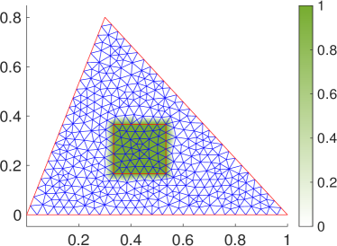
(a) Vorticity actuator. $M_{\sigma}=1$.

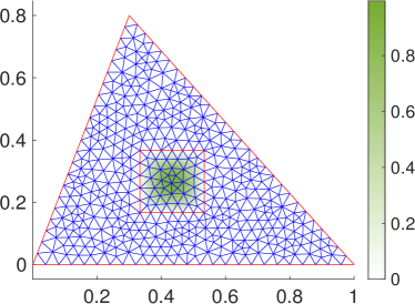
(b) Vorticity auxiliary function. $M_{\sigma}=1$

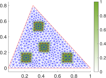
(c) Vorticity actuators. $M_{\sigma}=4$.

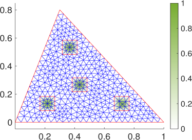
(d) Vorticity auxiliary functions. $M_{\sigma}=4$.

Figure 3. Triangulations ${\mathcal{T}}_{0}$, $M\in\{1,2\}$, and supports of the actuators.

Note that we used an ad-hoc geometry to including the boundary of the supports of the actuators. This is not essential, but provides (at least graphically) a better approximation of the actuators in coarse triangulations (cf. [29, Fig. 1]).

We consider regular refinements of these triangulations as

$${\mathcal{T}}_{\rho},\qquad\rho\in\{0,1,2\},$$

with ${\mathcal{T}}_{\rho+1}$ obtained from ${\mathcal{T}}_{\rho}$, $\rho\in\{0,1\}$, by dividing each triangle into $4$ similar triangles. We used the Matlab routines initmesh to generate ${\mathcal{T}}_{0}$ and refinemesh to generate ${\mathcal{T}}_{\rho+1}$.

Next, we consider the temporal (uniform) discretization of the interval $[0,+\infty)$ as

$${\mathbf{t}}\coloneqq t^{\rm step}{\mathbb{N}}=\{jt^{\rm step}\mid j\in{\mathbb{N}}\},\quad\mbox{with}\quad t^{\rm step}\coloneqq 4\cdot 10^{-4}$$

which we refine to arrive at the spatio-temporal discretizations, as

$${\mathbf{R}}_{\rho}\coloneqq({\mathcal{T}}_{\rho},{\mathbf{t}}_{\rho})\quad\mbox{with}\quad{\mathbf{t}}_{\rho}=2^{-\rho}{\mathbf{t}};\qquad\mbox{for}\quad\rho\in\{0,1,2\}.$$ (5.3)

Example 5.1.

We take the boundary and body external forcings as

$$g(t,x)=0,$$ (5.4a)

$$f(t,x)=2\cos(2t)\mathop{\rm sign}\nolimits(x_{1}-\tfrac{3}{10}+\tfrac{1}{10}\cos(4t))\mathop{\rm sign}\nolimits(x_{2}-\tfrac{3}{10}+\tfrac{1}{10}\sin(4t)).$$ (5.4b)

and the initial states as

$$w_{{\tt t}0}(x)=0,\qquad w_{0}(x)=-2\sin(3x_{1})+1.$$ (5.4c)

We considered the cases $M\in\{1,2\}$ and performed the simulations using the spatio-temporal mesh ${\mathbf{R}}_{\rho}$, with $\rho=1$.

In Fig. 4 we present the evolution of the free dynamics, corresponding to the case $\lambda=0$. We see that $w(t)$ converges exponentially to $w_{\tt t}(t)$. However, we recall that we want to check that an arbitrarily large decrease rate $\mu$ can be achieved; see Theorem 3.4. In the same Fig. 4 we can indeed see that a larger rate can be achieved by increasing $M$. For example, with $4$ actuators we obtain an exponential rate as $\mu\approx\tfrac{35}{20}=1.75$, whereas the stability rate of the free dynamics is approximately $\mu\approx\tfrac{16}{24}=0.66$. The oscillations that we see for time $t>20$ and $M=4$ is due to the fact that we have reached the used standard Matlab machine precision ${\tt eps}\approx 2\cdot 10^{-16}\approx{\mathrm{e}}^{-36}$.

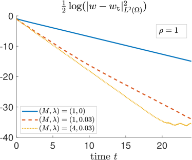
Figure 4. Increasing $M$. Data (5.4).

In Fig. 5 we present time-snapshots of the stream function of the targeted state. The associated velocity field is tangent to the plotted streamlines, pointing clockwise around a local maximum and counterclockwise around a local minimum.

In Fig. 6 we present time-snapshots of the stream function corresponding to the difference between the controlled $y$ and the targeted $y_{\tt t}$ states, and also time-snapshots of the stream function of the corresponding control forcing

$$Bu\coloneqq U_{M}^{\diamond}K_{M}^{\lambda}(w-w_{\tt t})\in{\mathcal{U}}_{M},$$

where in particular we can see the shape of the stream function of the actuator, with an extremum at the location of the support of its vorticity in Fig. 3(a).

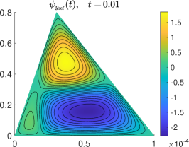
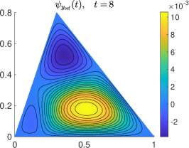
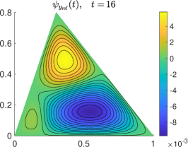
Figure 5. Stream function of the target. Data (5.4).

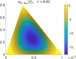
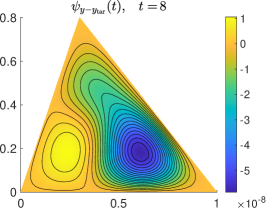
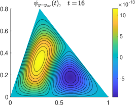
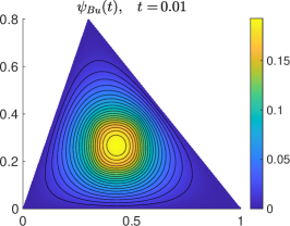
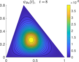
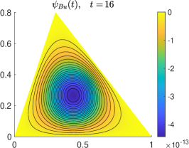
Figure 6. Stream functions of difference to target and control forcing. $M=1$. Data (5.4).

Next, in Fig. 7, we see the time-snapshots of the stream function for the case of $4$ actuators. In particular, from the stream function of the control forcing we can identify local extrema at the location of the supports of the vorticity of the actuators in Fig. 3(c).

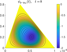
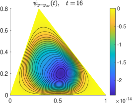
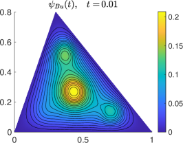
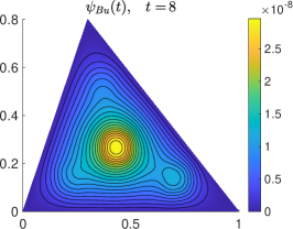
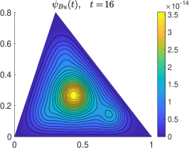
Figure 7. Stream function of difference to target and control forcing. $M=4$. Data (5.4).

Example 5.2.

Finally, we take ad-hoc initial data, in order to make the function

$$w_{\rm exa}(t,x)\coloneqq\sin(2t)(x_{1}-\tfrac{4}{10})$$

the exact solution of the free dynamics. Namely, we take the external forcings as

$$g(t,x)=w_{\rm exa}(t,x)\left.\kern-2.4pt\right|_{\partial\Omega},$$ (5.5a)

$$f(t,x)={\dot{w}_{\rm exa}}-\Delta w_{\rm exa}+\nu^{-1}\mathop{\rm curl}\nolimits^{*}(A^{-1}w_{\rm exa})\cdot\nabla w_{\rm exa},$$ (5.5b)

and the initial states as

$$w_{{\tt t}0}(x)=0,\qquad w_{0}(x)=-10\sin(3x_{1})\sin(4x_{2})+5.$$ (5.5c)

In Fig. 8 we confirm again that we can increase the exponential decrease rare of the differente to the target by increasing the number of actuators.

Finally, for the sake of completeness, and since we know the exact analytical expression of the targeted state, we compare the numerical solutions to the exact one. In Fig. 9 we consider the $3$ meshes in (5.3), and compare the computed targeted solution $w_{\tt t}$ with the exact one $w_{\rm exa}$ in Fig. 9(a). We can see that, in this example, that the solution computed in the coarsest mesh ${\mathbf{R}}_{0}$ gives us already a good approximation of $w_{\rm exa}$. We compare also the computed controlled solution $w$ to the exact one $w_{\rm exa}$ in Fig. 9(b).

Finally, we would like to underline that the exact analytical expression for $w_{\rm exa}$ was used at the plotting stage only. The control input $u(t)=K_{M}^{\lambda}(w(t)-w_{\tt t}(t))\in{\mathbb{R}}^{M_{\sigma}}$ was computed based on the difference between the numerical controlled $w$ and the numerical targeted $w_{\tt t}$ trajectories. That is, in the computations we did not use the fact that we know $w_{\rm exa}$; we used only the knowledge of the data tuple $(f,g,w_{{\tt t}0},w_{0})$.

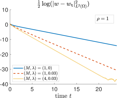
Figure 8. Increasing $M$. Data (5.5).

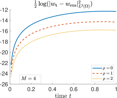
(a) Numerical error between computed and exact targeted vorticity.

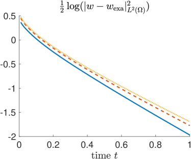
(b) Difference between computed controlled vorticity and exact targeted vorticity.

Figure 9. On the refinement level of the discretization. Data (5.5).

Remark 5.3.

We can reduce the case nonhomogeneous boundary conditions to the homogeneous one if $g$ is regular enough. For example, in case we have $g=G\left.\kern-2.4pt\right|_{\partial\Omega}$ with $G$ smooth in the closed cylinder $[0,+\infty)\times\overline{\Omega}$. Then $w^{0}\coloneqq w-G$ will satisfy the homogeneous boundary conditions and a dynamics analogue to (5.1a) with some different data $(f,w_{{\tt t}0})$ and some extra linear terms involving $G$. The arguments we followed in previous sections can be adapted to this dynamics by taking care of the extra linear terms by including them in the operator $A_{\rm rc}$ in (4.2). We refer the reader to [24, Def. 5.2], where such a lifting argument $g\mapsto G$ has been used.

Remark 5.4.

In both Examples 5.1 and 5.2 we see that the free dynamics of the difference to the target is exponentially stable. This suggests that the free dynamics is stable in a neighborhood of the considered targets. We would like to say that we do not know whether this is the case in our setting with Lions boundary conditions in a triangular domains; though, we suspect that it is not. For example, we recall that this is not the case for periodic boundary conditions, as we can see from the works in [22, 33]. From these works we can also see that proving the instability around a given steady state is a nontrivial task, and may require to take $\nu$ small enough (for a fixed “normalized” steady state) [33, Thm. 2.9]. Note also that a smaller $\nu$ requires a finer discretization which means that numerical computations can become very expensive or unfeasible.

6. Concluding remarks and potential developments

We have shown that, given an arbitrary $\mu>0$, we can find a finite set of actuators $\Phi_{i}$ each with vorticity localized in a small domain $\omega_{i}$ which enable us to stabilize, with exponential rate $\mu$, the 2D Navier–Stokes system to a given velocity field trajectory $y_{\tt t}$ of the free dynamics. The input control is given by an explicit linear feedback operator based on suitable oblique projections.

6.1. On the 3D Navier–Stokes equations

It is well known that in the case of spatial domains  $\Omega\subset{\mathbb{R}}^{3}$ the analysis of the 3D Navier–Stokes equations is more involved. In fact, the well-posedness of the Cauchy problem on existence, uniqueness, and continuity of the solutions on the initial data is still an open problem, for large time intervals. Another point is that the vorticity is not anymore a scalar function, but a vector

$$w=\mathop{\rm Curl}\nolimits y\coloneqq(\mathop{\rm curl}\nolimits_{(x_{2},x_{3})}(y_{2},y_{3}),\mathop{\rm curl}\nolimits_{(x_{3},x_{1})}(y_{3},y_{1}),\mathop{\rm curl}\nolimits_{(x_{1},x_{2})}(y_{1},y_{2})),$$

for a velocity field $y(x)\eqqcolon(y_{1},y_{2},y_{3})(x)$, with the generalization of $\mathop{\rm curl}\nolimits$ in (1.2) as

$$\mathop{\rm curl}\nolimits_{(a,b)}(f_{1},f_{2})\coloneqq\tfrac{\partial}{\partial b}f_{1}-\tfrac{\partial}{\partial a}f_{2}.$$

The dynamics of the vorticity is given by a system of three scalar parabolic equations

$$\dot{w}_{\tt t}-\nu\Delta w_{\tt t}+y_{\tt t}\cdot\nabla w_{\tt t}+w_{\tt t}\cdot\nabla y_{\tt t}=\mathop{\rm curl}\nolimits f,\qquad w_{\tt t}(0)=w_{{\tt t}0},$$

instead of the single one (3.2) that we have the 2D case. The Lions boundary conditions ${\mathcal{G}}y_{\tt t}\left.\kern-2.4pt\right|_{\partial\Omega}=0$ also take the more cumbersome expression in the 3D case as

$${\mathcal{G}}=(y_{\tt t}\cdot{\mathbf{n}},\mathop{\rm Curl}\nolimits y_{\tt t}-((\mathop{\rm Curl}\nolimits y_{\tt t})\cdot{\mathbf{n}}){\mathbf{n}});$$

see [34]. That is, now the vorticity is normal to the boundary, but not necessarily vanishing as in the 2D case; see (1.3).

Thus, though the possibility of derivation of an analogue stabilizability result seems plausible, it will involve considerable extra work in order to overcome the new regularity issues. In particular, we can see that within the proofs of Lemmas 4.3 and 4.4 we have used arguments (e.g., Sobolev embeddings) which do not hold (exactly in the same way) in the 3D case. Due to the importance of the 3D case in a wider range of real-world applications, it would be interesting to investigate derivation of such an analogue stabilizability result a future work.

6.2. On the “localized” actuators

We have considered actuators with vorticity locally supported in small subdomains with the same shape, up to a translation and a rotation. In the literature we often find actuators taken as solenoidal projections of locally supported vector fields, for example, in the 2D case as the vector fields

$$\widehat{\Phi}_{i_{1}}^{\bullet}\coloneqq 1_{\omega_{i}}(1,0),\qquad\widehat{\Phi}_{i_{2}}^{\bullet}\coloneqq 1_{\omega_{i}}(0,1),\qquad 1\leq i\leq M;$$ (6.1)

supported in subdomains $\omega_{i}\subset\Omega$, $\omega_{i}\neq\Omega$, of the spatial domain $\Omega$; see [4, Sect. 4, Exa. 2]. See also [4, Sect. 4, Exa. 2], [11, Eqs. (1.1) and (1.4)] and [10, Sect. 3], where other locally supported vector fields are taken.

Actuators as in (6.1) are in $(L^{2}(\Omega))^{2}$, but are not in the state space ${\mathbf{H}}$ of solenoidal vector fields and their Leray projections $\widehat{\Phi}_{i_{j}}\coloneqq\Pi\widehat{\Phi}_{i_{j}}^{\bullet}$ onto ${\mathbf{H}}$ depends on $\Omega$ (because $\Pi$ depends on $\Omega$). Analogously, for the actuators $\Phi_{i}$ considered in this manuscript, say with localized vorticity $\mathop{\rm curl}\nolimits\Phi_{i}=1_{\omega_{i}}$, we can see that  $\Phi_{i}=\mathop{\rm curl}\nolimits^{*}A^{-1}1_{\omega_{i}}$ also depends on $\Omega$ (because $A$ depends on $\Omega$). Thus, neither of the actuators are localized, in the sense that neither $\widehat{\Phi}_{i_{j}}$ nor $\Phi_{i}$ can be constructed independently of $\Omega$. This observation raises the following question, which could be important for applications: can we find a family of stabilizing actuators, in ${\mathbf{H}}$ and supported in small subdomains, which can be constructed (manufactured) independently of $\Omega$? The investigation of this question is an interesting subject for future work.

6.3. On output based feedback stabilization

We have seen in Section 1.3 that the feedback control system that we propose can be interpreted as a Luenberger observer, thus our strategy can be applied to state estimation (also known as continuous data assimilation [5]). We can construct a set of sensors and a set of actuators as a slight variation of the construction in Section 2.2. Namely, putting a sensor besides an actuator instead of just an actuator/sensor as in Figs. 1 and 2. This has been done in [27, Fig. 1], where a feedback control was coupled with an observer to achieve an output-based stabilization result in the case of linear dynamics. The extension of such a result for general nonlinear dynamics is a nontrivial problem, because the so-called separation principle does not hold, in general. However, the investigation of this problem is of paramount importance for real world applications. In particular, the derivation of results on this direction concerning the nonlinear Navier–Stokes equations is an interesting subject for future research.

Aknowlegments. D. Seifu was supported by the State of Upper Austria and the Austrian Science Fund (FWF): P 33432-NBL, S. Rodrigues acknowledges partial support from the same grant.

References

- [1] S. Agmon. Lectures on Elliptic Boundary Value Problems. Van Nostrand, 1965. reprinted by AMS 2010. doi:10.1090/chel/369.
- [2] C. Amrouche and A. Rejaiba. -theory for Stokes and Navier–Stokes equations with Navier boundary condition. J. Differential Equations, 256(4):1515–1547, 2014. doi:10.1016/j.jde.2013.11.005.
- [3] G. Auchmuty and J.C. Alexander. -well-posedness of planar div-curl systems. Arch. Ration. Mech. Anal., 160(2):91–134, 2002. doi:10.1007/s002050100156.
- [4] B. Azmi. Stabilization of 3D Navier–Stokes equations to trajectories by finite-dimensional RHC. Appl. Math. Optim., 86(3):art38, 2022. doi:10.1007/s00245-022-09900-0.
- [5] A. Azouani, E. Olson, and E. S. Titi. Continuous data assimilation using general interpolant observables. J. Nonlinear Sci., 24(2):277–304, 2014. doi:10.1007/s00332-013-9189-y.
- [6] A. Azouani and E.S. Titi. Feedback control of nonlinear dissipative systems by finite determining parameters – a reaction-diffusion paradigm. Evol. Equ. Control Theory, 3(4):579–594, 2014. doi:10.3934/eect.2014.3.579.
- [7] M. Badra and T. Takahashi. Stabilization of parabolic nonlinear systems with finite dimensional feedback or dynamical controllers: Application to the Navier–Stokes system. SIAM J. Control Optim., 49(2):420–463, 2011. doi:10.1137/090778146.
- [8] V. Barbu. Stabilization of navier–stokes equations by oblique boundary feedback controllers. SIAM J. Control Optim., 50(4):2288–2307, 2012. doi:10.1137/110837164.
- [9] V. Barbu and I. Munteanu. Internal stabilization of Navier–Stokes equation with exact controllability on spaces with finite codimension. Evol. Equ. Control Theory, 1(1):1–16, 2012. doi:10.3934/eect.2012.1.1.
- [10] V. Barbu, S.S. Rodrigues, and A. Shirikyan. Internal exponential stabilization to a nonstationary solution for 3D Navier–Stokes equations. SIAM J. Control Optim., 49(4):1454–1478, 2011. doi:10.1137/100785739.
- [11] V. Barbu and R. Triggiani. Internal stabilization of Navier–Stokes equations with finite-dimensional controllers. Indiana Univ. Math. J., 53(5):1443–1494, 2004. doi:10.1512/iumj.2004.53.2445.
- [12] H. Beirão da Veiga and F. Crispo. Sharp inviscid limit results under Navier type boundary conditions. an theory. J. Math. Fluid. Mech., 12(3):397–411, 2010. doi:10.1007/s00021-009-0295-4.
- [13] L.C. Berselli and S. Spirito. On the vanishing viscosity limit of 3d Navier–Stokes equations under slip boundary conditions in general domains. Commun. Math. Phys., 316(1):171–198, 2012. doi:10.1007/s00220-012-1581-1.
- [14] N.V. Chemetov, F. Cipriano, and S. Gavrilyuk. Shallow water model for lakes with friction and penetration. Math. Meth. Appl. Sci., 33(6):687–703, 2010. doi:10.1002/mma.1185.
- [15] T. Clopeau, A. Mikelić, and R. Robert. On the vanishing viscosity limit for the 2D incompressible Navier–Stokes equations with the friction type boundary conditions. Nonlinearity, 11(6):1625–1636, 1998. doi:doi:10.1088/0951-7715/11/6/011.
- [16] J.-M. Coron. On the controllability of the 2-D incompressible Navier–Stokes equations with the Navier slip boundary conditions. ESAIM Control Optim. Calc. Var., 1:35–75, 1996. doi:10.1051/cocv:1996102.
- [17] F. Demengel and G. Demengel. Functional Spaces for the Theory of Elliptic Partial Differential Equations. Universitext. Springer, 2012. doi:10.1007/978-1-4471-2807-6.
- [18] J. P. Kelliher. Navier–Stokes equations with Navier boundary conditions for a bounded domain in the plane. SIAM J. Math. Anal., 38(1):210–232, 2006. doi:10.1137/040612336.
- [19] K. Kunisch, S. S. Rodrigues, and D. Walter. Learning an optimal feedback operator semiglobally stabilizing semilinear parabolic equations. Appl. Math. Optim., 84(S1):277–318, 2021. doi:10.1007/s00245-021-09769-5.
- [20] K. Kunisch and S.S. Rodrigues. Explicit exponential stabilization of nonautonomous linear parabolic-like systems by a finite number of internal actuators. ESAIM Control Optim. Calc. Var., 25:art67, 2019. doi:10.1051/cocv/2018054.
- [21] J.-L. Lions. Quelques Méthodes de Résolution des Problèmes aux Limites Non Linéaires. Dunod et Gauthier–Villars, Paris, 1969.
- [22] V.X. Liu. Instability for the Navier–Stokes equations on the 2-dimensional torus and a lower bound for the Hausdorff dimension of their global attractors. Commun. Math. Phys., 147(2):217–230, 1992. doi:10.1007/BF02096584.
- [23] D. Phan and S.S. Rodrigues. Gevrey regularity for Navier–Stokes equations under Lions boundary conditions. J. Funct. Anal., 272(7):2865–2898, 2017. doi:10.1016/j.jfa.2017.01.014.
- [24] S. S. Rodrigues. Local exact boundary controllability of 3D Navier–Stokes equations. Nonlinear Anal., 95:175–190, 2014. doi:10.1016/j.na.2013.09.003.
- [25] S.S. Rodrigues. Feedback boundary stabilization to trajectories for 3d navier–stokes equations. Appl. Math. Optim., 84(S2):1149–1186, 2021. doi:10.1007/s00245-017-9474-5.
- [26] S.S. Rodrigues. Oblique projection exponential dynamical observer for nonautonomous linear parabolic-like equations. SIAM J. Control Optim., 59(1):464–488, 2021. doi:10.1137/19M1278934.
- [27] S.S. Rodrigues. Oblique projection output-based feedback stabilization of nonautonomous parabolic equations. Automatica J. IFAC, 129:art109621, 2021. doi:10.1016/j.automatica.2021.109621.
- [28] S.S. Rodrigues. Semiglobal oblique projection exponential dynamical observers for nonautonomous semilinear parabolic-like equations. J. Nonlinear Sci., 31:art100, 2021. doi:10.1007/s00332-021-09756-8.
- [29] S.S. Rodrigues. Stabilization of nonautonomous linear parabolic-like equations: oblique projections versus Riccati feedbacks. Evol. Equ. Control Theory, 12(2):647–686, 2022. doi:10.3934/eect.2022045.
- [30] S.S. Rodrigues and K. Sturm. On the explicit feedback stabilisation of one-dimensional linear nonautonomous parabolic equations via oblique projections. IMA J. Math. Control Inform., 37(1):175–207, 2020. doi:10.1093/imamci/dny045.
- [31] R. Temam. Infinite-Dimensional Dynamical Systems in Mechanics and Physics. Number 68 in Appl. Math. Sci. Springer, 2nd edition, 1997. doi:10.1007/978-1-4612-0645-3.
- [32] R. Temam. Navier–Stokes Equations: Theory and Numerical Analysis. AMS Chelsea Publishing, Providence, RI, reprint of the 1984 edition, 2001. URL: https://bookstore.ams.org/chel-343-h.
- [33] S. Vasudevan. Instability of unidirectional flows for the 2D Navier–Stokes equations and related -models. J. Math. Fluid Mech., 23(2):art35, 2021. doi:10.1007/s00021-021-00568-0.
- [34] Y. Xiao and Z. Xin. On the vanishing viscosity limit for the 3D Navier–Stokes equations with a slip boundary condition. Comm. Pure Appl. Math., 60(7):1027–1055, 2007. doi:10.1002/cpa.20187.