Reheating constraints on modified quadratic chaotic inflation

Abstract

The Reheating era of inflationary Universe can be parameterized by various parameters like reheating temperature $T_{\text{re}}$, reheating duration $N_{\text{re}}$ and average equation of state parameter $\overline{\omega}_{\text{re}}$, which can be constrained by observationally feasible values of scalar power spectral amplitude $A_{\text{s}}$ and spectral index $n_{\text{s}}$. In this work, by considering the quadratic chaotic inflationary potential with logarithmic-correction in mass, we examine the reheating era in order to place some limits on model’s parameter space. By investigating the reheating epoch using Planck’s 2018 data, we show that even a small correction can make the quadratic chaotic model consistent with latest cosmological observations. We also find that the study of reheating era helps to put much tighter constraints on model and effectively improves accuracy of model.

1 Introduction

The inflationary paradigm [1, 2, 3, 4, 5] is an exciting and influential epoch of the cosmological universe. It has come up as an aid to resolve a range of well-known cosmological problems like flatness, horizon and monopole problems of famous cosmological big bang theory. The semi-classical theory of inflation generates seeds for Cosmic Microwave Background anisotropy and Large Scale Structures in the late universe [6, 7, 8]. Inflation predicts adiabatic, gaussian and almost scale invariant density fluctuations, which are validated by CMB observations like Cosmic Background Explorer (COBE) [9], Wilkinson Microwave Anisotropy Probe (WMAP) [10, 11] and Planck space probe [12, 13, 14, 15, 16, 17].

In the realm of inflationary cosmology, a typical scenario involves the presence of a scalar field, which is referred to as the inflaton $(\phi)$, whose potential energy dominates the universe. In this picture, inflaton slowly rolls through its potential, and the coupling of quantum fluctuations of this scalar field with metric fluctuations is the source of primordial density perturbations called scalar perturbations. The tensor part of the metric has vacuum fluctuations resulting in primordial gravitational waves called tensor perturbations. During inflation, power spectra for both these perturbations depend on a potential called inflaton potential $V(\phi)$.

As Inflation ends, the universe reaches a highly nonthermal and frigid state with no matter content in it. However, the universe must be thermalized at extremely high temperature for big-bang nucleosynthesis (BBN) and baryogenesis. This is attained by ‘reheating’[18, 19, 20, 21, 22, 23, 24], transit between the inflationary phase and an era of radiation and matter dominance.

There is no established science for reheating era and there is also a lack of direct observational data in favor of reheating. However, recent CMB data helped to obtain indirect bounds for various reheating parameters [25, 26, 27, 28, 29, 30, 31], and those parameters are: the reheating temperature $\left(T_{\text{re}}\right)$, the effective equation of state (EoS) parameter during reheating ($\omega_{\text{re}}$) and lastly, the reheating duration, which can be written in the form of number of e-folds $\left(N_{\text{re}}\right.$). It is challenging to bound the reheating temperature by LSS and CMB observations. However, its value is assumed to be higher than the electroweak scale for dark matter production at a weak scale. A lower limit has been set on reheat temperature i.e. $\left(T_{\text{re}}\sim 10^{-2}GeV\right.$) for a successful primodial nucleosynthesis (BBN) [32] and instantaneous reheating consideration allows us to put an upper bound i.e. $\left(T_{\text{re}}\sim 10^{16}GeV\right.$) for Planck’s recent upper bound on tensor-to-scalar ratio (r). The value of second parameter, $\omega_{\text{re}}$, shifts from $-\frac{1}{3}$ to 1 in various scenarios. It is 0 for reheating generated by perturbative decay of a large inflaton and $\frac{1}{3}$ for instantaneous reheating. The next parameter in line is the duration of reheating phase, $N_{re}$. Generally, it is incorporated by giving a range of $N_{k}$, the number of e-foldings from Hubble crossing of a Fourier mode $k$ to the termination of inflation. $N_{k}$ has value in the range 46 to 70 in order to work out the horizon problem. These bounds arise by considering reheat temperature at electroweak scale and instantaneous reheating of the universe. A comprehensive analysis of higher bound on $N_{k}$ is presented in [33, 34].

The relation between inflationary parameters and reheating can be derived by taking into consideration the progression of observable scales of cosmology from the moment of their Hubble crossing during inflation to the current time. We can deduce relations among $T_{\text{re}},N_{\text{re}}$ and $\omega_{\text{re}}$, the scalar power spectrum amplitude $\left(A_{s}\right.$) and spectral index $n_{s}$ for single-field inflationary models. Further, the constraints on $T_{\text{re}}$ and $N_{\text{re}}$ can be obtained from recent CMB data.

Although plenty of inflationary models have been studied in recent years[35] and the inflationary predictions are in agreement with the recent CMB observations, there is still a need for a unique model. The most famous chaotic inflation with quadratic potential $\left(\frac{1}{2}m^{2}\phi^{2}\right)$ is eliminated by recent cosmological observations as it predicts large tensor perturbations due to large potential energy it has during inflaton at large field amplitudes. Hence, lowering the potential at higher field values can help getting rid of this obstacle. Numerous hypotheses in this vein have been put forth [36, 37, 38, 39, 40, 41, 42, 43, 44, 45]. Radiative corrections provide an intriguing possibility [36, 37, 38] where, generally, the quadratic potential gets flatter as result of running of inflaton’s quartic coupling. This article will rather examine a straightforward scenario in which the mass exhibits a running behaviour described as [46]:

$$m^{2}(\phi)=m^{2}\left(1-\text{K}\ln\left[\frac{\phi^{2}}{M^{2}}\right]\right),$$ (1)

where M is large mass scale and K is some positive constant. The positive K and the negative sign in above equation is a defining characteristic of dominance of the coupling of inflaton field to fermion fields. Another interesting way to make such models compatible with observations is by extension of standard model as done in Ref. [47, 48].
Reheating is well known technique of constraining the inflationary models. There are various ways to analyse the reheating phase as available in literature e.g. one stage reheating study [49, 31], two stage reheating study [50, 51]. In Ref. [52] reheating was analysed through perturvative decay of inflaton to either bosonic or fermionic states through trilinear coupling [52]. Considering one stage reheating technique of constraining the models, we use various reheating parameters to put much tighter bounds on parameter space of quadratic chaotic inflationary model with a logarithmic-correction in mass in light of Planck’s 2018 data [16, 17]. By demanding $T_{\text{re}}>100$ GeV for production of weak-scale dark matter and working in plausible range of average equation of state (EoS) parameter ($-\frac{1}{3}\leq\overline{\omega}_{\text{re}}\leq 1$), we employ the derived relation between inflationary and reheating parameters and observationally feasible values of $A_{s}$, $n_{s}$ and r to place a limit on model’s parameter space. It is a helpful and fairly new tool for putting relatively tighter constraints on the model and reducing its viable parameter space, providing significant improvement in accuracy of the model. Additionally, this technique well differentiate various inflation models as they can have the same forecasts for $n_{s}$ and r, but definitely not for the same $\omega_{\text{re}}$, as the tightened constraints on $n_{s}$ will result in an increasingly narrow permitted range of $\omega_{\text{re}}$ for a particular inflationary model.

The organization of this paper is as follows: In Sec. 2 we discuss the dynamics and predictions of slow-roll inflation. We also derived the expressions for $T_{\text{re}}$ and $N_{\text{re}}$ as a function of $\overline{\omega}_{\text{re}}$ and other inflationary parameters like ($\text{$\Delta$N}_{k}$ and $V_{\text{end}}$). In section 3, the Subsec. 3.1 has our recreated data for reheating scenario of simple quadratic chaotic potential. In Subsec. 3.2, we discussed the various field domains within which inflation can occur for quadratic chaotic potential with logarithmic correction in mass and then we parameterized reheating for this model using $T_{\text{re}}$ and $N_{\text{re}}$ as a function of the scalar spectral index $n_{s}$ for different $\omega_{\text{re}}$. We have also examined the observational limits and reheating parameters for both these models using Planck 2018 data in Sec. 3. Sec. 4 is reserved for discussion and conclusions.

We will be working with $\hbar$ $=c=1$ units and the values of some standard parameters used are reduced Planck’s mass $M_{P}=\sqrt{\frac{1}{8\pi G}}$ $=\text{}$2.435 $\times$ $10^{18}$ GeV, the redshift of matter radiation equality $z_{\text{eq}}=$3402, $g_{\text{re}}$ $\approx$ 100 [27] and the present value of Hubble parameter $H_{o}=100$h km $s^{-1}$ $\text{Mpc}^{-1}$ with h = 0.68 [16, 17]

2 Parameterizing reheating in slow-roll inflationary models

Reheating phase can be parameterized by assuming it been dominated by some fluid [53] of energy density $\rho$ with pressure P and equation of state(EoS) parameter $\omega_{\text{re}}=\frac{P}{\rho}$ where

$$\rho=\frac{\dot{\phi}^{2}}{2}+V(\phi),\;\;\;\;\;\;\;\;\;P=\frac{\dot{\phi}^{2}}{2}-V(\phi).$$ (2)

The continuity equation gives

$$\dot{\rho}+3H(P+\rho)=0,$$ (3)

$$\dot{\rho}+3H\rho\left(\omega_{\text{re}}+1\right)=0.$$ (4)

We analyze the dynamics of inflation by considering inflaton $\phi$ with potential $V(\phi)$ evolving slowly with slow-roll parameters $\epsilon$ and $\eta$. The approximation of Friedman equation using slow-roll conditions give

$$3H\dot{\phi}+V^{\prime}(\phi)=0,$$ (5)

$$H^{2}=\frac{V(\phi)}{3M_{P}^{2}},$$ (6)

where prime$(^{\prime})$ denotes derivative w.r.t $\phi$ and H = $\frac{\dot{a}}{a}$ is Hubble parameter. The definition of slow-roll parameter give

$$\epsilon=\frac{M_{P}^{2}}{2}\left(\frac{V^{\prime}}{V}\right)^{2},\;\;\;\;\;\;\;\;\;\;\;\eta=M_{P}^{2}\left(\frac{V^{\prime\prime}}{V}\right).$$ (7)

The scalar spectral index $n_{s}$, tensor spectral index $n_{T}$ and tensor to scalar ratio $r$ in terms of above slow-roll parameters satisfy the relations

$$\text{ }n_{s}=1-6\epsilon+2\eta,\;\;\;\;\;\;\;n_{T}=-2\epsilon,\;\;\;\;\;\;\;r=16\epsilon.$$ (8)

Now, the number of e-foldings in between Hubble crossing of mode $k$ and termination of inflation denoted by subscript “end” can be given as

$$\Delta N_{k}=\ln\left(\frac{a_{\text{end}}}{a_{\text{k}}}\right)=\frac{1}{M_{P}^{2}}\int_{\phi_{\text{end}}}^{\phi_{k}}\frac{V}{V^{\prime}}\,d\phi,$$ (9)

where $a_{k}$ and $\phi_{k}$ represents value of scale factor and inflaton at the point of time when $k$ crosses the Hubble radius. The later part of eq. (9) is obtained using the slow-roll approximations $\ddot{\phi}\ll 3H\dot{\phi}$ and $V(\phi)\gg\dot{\phi}^{2}$. Similarly,

$$N_{\text{re}}=\ln\left(\frac{a_{\text{re}}}{a_{\text{end}}}\right),$$ (10)

Here the quantity $N_{\text{re}}$ encrypts both, an era of preheating [22, 54, 55, 56, 57, 58] as well as later thermalization process. An energy density controls the Universe’s subsequent evolution and can be written as

$$\text{ }\rho_{\text{re}}=\frac{\pi^{2}}{30}g_{\text{re}}T_{\text{re}}^{4},$$ (11)

where $g_{\text{re}}$ gives the actual count of relativistic species at termination of reheating epoch and $T_{\text{re}}$ is the reheating temperature. Now, in view of eq. (3)

$$\rho_{\text{re}}=\rho_{\text{end}}e^{-3N_{\text{re}}\left(1+\overline{\omega}_{\text{re}}\right)},$$ (12)

$$\text{where }{}{}\overline{\omega}_{\text{re}}=<\omega>=\frac{1}{N_{\text{re}}}\int_{N_{\text{end}}}^{N}\omega_{\text{re}}(N)dN,$$ (13)

Here $\overline{\omega}_{\text{re}}$ is average EoS parameter during reheating [25, 49]. Now, eq. (12) can be recast as

$$\frac{a_{\text{re}}}{a_{\text{end}}}=e^{N_{\text{re}}}=\left(\frac{\rho_{\text{re}}}{\rho_{\text{end}}}\right)^{-\frac{1}{3(1+\overline{\omega}_{\text{re}})}}.$$ (14)

Using eq. (11) and eq. (14), reheating e-folds $N_{\text{re}}$ can be written as

$$N_{\text{re}}=\frac{1}{3\left(1+\overline{\omega}_{\text{re}}\right)}\left\{\ln\left(\frac{3}{2}V_{\text{end}}\right)-\ln\left(\frac{\pi^{2}}{30}g_{\text{re}}\right)\right\}-\frac{4}{3\left(1+\overline{\omega}_{\text{re}}\right)}\ln\left(T_{\text{re}}\right).$$ (15)

For some physical scale $k$, the observed wavenumber ‘$\frac{k}{a}$’ can be given in terms of above known quantities and the redshift during matter-radiation equality epoch ($z_{\text{eq}}$) as [49]

$$H_{k}=\frac{k}{a_{k}}=\left(1+z_{\text{eq}}\right)\frac{k}{a_{o}}\rho_{\text{re}}^{\frac{3~{}\overline{\omega}_{\text{re}}-1}{12\left(1+\overline{\omega}_{\text{re}}\right)}}\rho_{\text{eq}}{}^{-\frac{1}{4}}\left(\frac{3}{2}V_{\text{end}}\right)^{\frac{1}{3\left(1+\overline{\omega}_{\text{re}}\right)}}e^{\Delta N_{k}}.$$ (16)

Using eq. (16), $\Delta N_{k}$ can be given as

$$\Delta N_{k}=\ln H_{k}-\ln\left(1+z_{\text{eq}}\right)-\ln\left(\frac{k}{a_{o}}\right)-\frac{1}{\left.3(\overline{\omega}_{\text{re}}+1\right)}\ln\left(\frac{3}{2}V_{\text{end}}\right)-\frac{3~{}\overline{\omega}_{\text{re}}-1}{3\left(1+\overline{\omega}_{\text{re}}\right)}\ln\left(\rho_{\text{re}}^{\frac{1}{4}}\right)+\ln\left(\rho_{\text{eq}}^{\frac{1}{4}}\right).$$ (17)

Inverting eq. (17), and using eq. (11) one can get a mutual relation among the numerous parameters introduced,

$$\ln(T_{\text{re}})=\frac{3~{}\left(1+\overline{\omega}_{\text{re}}\right)}{3~{}\overline{\omega}_{\text{re}}-1}\left\{\ln H_{k}-\ln\left(1+z_{\text{eq}}\right)-\ln\frac{k}{a_{o}}-\Delta N_{k}+\ln\left(\rho_{\text{eq}}^{\frac{1}{4}}\right)\right\}-\frac{1}{3~{}\overline{\omega}_{re}-1}\ln\left(\frac{3}{2}V_{end}\right)-\frac{1}{4}\ln\left(\frac{\pi^{2}}{30}g_{re}\right).$$ (18)

The expression for $T_{\text{re}}$ from eq. (15) is substituted in eq. (18) to get the expression for $N_{\text{re}}$ as mentioned below

$$N_{\text{re}}=\frac{1}{3~{}\overline{\omega}_{\text{re}}-1}\ln\left(\frac{3}{2}V_{\text{end}}\right)+\frac{4}{3~{}\overline{\omega}_{\text{re}}-1}\left\{\ln\left(\frac{k}{a_{o}}\right)+\Delta N_{k}+\ln\left(1+z_{\text{eq}}\right)-\ln\left(\rho_{\text{eq}}^{\frac{1}{4}}\right)-\ln H_{k}\right\}.$$ (19)

eq. (18) and eq. (19) are the two key relationships for parameterizing reheating in slow-roll inflationary models.

3 Inflationary models

3.1 Quadratic Chaotic inflationary model

We are first considering simple quadratic chaotic potential before moving to its modified form. The quadratic chaotic potential [4] has the form

$$V=\frac{1}{2}m^{2}\phi^{2}.$$ (20)

The reheating study of this potential was already done in [49] in light of Planck’s 2015 data, we are recreating the data by doing the similar study using Planck’s 2018 data. Using eq. (7) slow-roll parameters for this potential can be given as

$$\epsilon=\eta=\frac{2M_{P}^{2}}{\phi^{2}}.$$ (21)

The Hubble parameter during the crossing of Hubble radius by scale $k$ for this model can be written as

$$H_{k}^{2}=\frac{1}{M_{P}^{2}}\left(\frac{V_{k}}{3-\epsilon_{k}}\right)=\frac{1}{2M_{P}^{2}}\left(\frac{m^{2}\phi_{k}^{2}}{3-2\frac{M_{P}^{2}}{\phi^{2}}}\right).$$ (22)

where $\phi_{k}$, $\epsilon_{k}$ and $V_{k}$ respectively represent the inflaton field, slow-roll parameter and potential during crossing of Hubble radius by mode $k$.
Using the condition $\epsilon=1$, defining end of inflation, in eq. (21), we obtained $\frac{\phi_{\text{end}}^{2}}{M_{P}^{2}}=2$
Now, corresponding to pivot scale $k_{*}$, used in Planck collaboration, $\frac{k_{*}}{a_{o}}=0.05Mpc^{-1}$, consider the mode $k_{*}$ crossing the hubble radius at a point where the field has achieved the value $\phi_{*}$ during inflation. The remaining number of e-folds persist subsequent to crossing of hubble radius by $k_{*}$ are

$$\Delta N_{*}\simeq\frac{1}{M_{P}^{2}}\int_{\phi_{\text{end}}}^{\phi_{*}}\frac{V}{V^{\prime}}\,d\phi\\ \\ =\left[\left(\frac{\phi_{*}}{2M_{P}}\right)^{2}-\frac{1}{2}\right].$$ (23)

The spectral index for this model can be easily obtained using eq. (8) as

$$n_{s}=1-8\left(\frac{M_{P}^{2}}{\phi_{*}^{2}}\right).$$ (24)

Now, the formulation for tensor-to-scalar ratio from eq. (8) gives

$$r=32\frac{M_{P}^{2}}{\phi_{*}^{2}}.$$ (25)

Moreover, this model yields the relation

$$H_{*}=\pi M_{P}\sqrt{16A_{s}\frac{M_{P}^{2}}{\phi_{*}^{2}}}.$$ (26)

The relation of field $\phi$ and $H$ eq. (6), and the condition for termination of inflation as used in eq. (23), along with eq. (26) gives expression for $V_{\text{end}}$ as

$$V_{\text{end}}(\phi)=\frac{1}{2}m^{2}\phi_{\text{end}}^{2}=\frac{3H_{*}^{2}M_{P}^{2}\phi_{\text{end}}^{2}}{\phi_{*}^{2}}=\frac{6H_{*}^{2}M_{P}^{4}}{\phi_{*}^{2}}.$$ (27)

Figure 1: The plots for (a) $T_{\text{re}}$ and (b) $N_{\text{re}}$ versus $n_{s}$ for the quadratic chaotic model $V(\phi)=\frac{1}{2}m^{2}\phi^{2}$ for different values of $\overline{\omega}_{\text{re}}$ : $\overline{\omega}_{\text{re}}$=$-\frac{1}{3}$(dotted orange), $\overline{\omega}_{\text{re}}$= 0(medium dashed purple), $\overline{\omega}_{\text{re}}$=$\frac{1}{6}$(solid green), $\overline{\omega}_{\text{re}}$=$\frac{2}{3}$(large dashed red), $\overline{\omega}_{\text{re}}$= 1(small dashed blue). The regions with light and dark gray shades represent the Planck 2018 (TE+EE+TT+Low E+Lensing) [16, 17] 2$\sigma$ and 1$\sigma$ bounds on $n_{s}$ respectively.

Now, the expressions for $\Delta$$N_{*}$, $r$, $H_{*}$ and $V_{\text{end}}$ as a function of $n_{s\text{ }}$ can be obtained by putting the value of $\phi_{*}$ from eq. (24) in eqs. (23), (25), (26) and (27), and then these expressions along with eqs. (18) and (19) gives number of reheating e-folds $N_{\text{re}}$ and reheating temperature $T_{\text{re}}$. Planck’s 2018 value of $\text{ }A_{s}=2.1\times 10^{-9}$ and computed value of $\rho_{\text{eq}}^{\frac{1}{4}}=10^{-9}$GeV [16, 17] have been used for calculation. The $N_{\text{re}}$ and $T_{\text{re}}$ versus $n_{s}$ plots, along with Planck-2018 $1\sigma$ bound on $n_{s}$ i.e. $n_{s}\text{=0.965$\pm$0.004}$ (dark gray) and $2\sigma$ bound on $n_{s}$ i.e. $n_{s}\text{=0.965$\pm$0.008}$ (light gray), for this model are presented graphically in figure 1 for a range of average EoS parameter during reheating.
By demanding $T_{\text{re}}\geq 100$ GeV for production of weak-scale dark matter and solving eqs. (18) and (24), the bounds on $n_{s}$ are obtained and are reflected on eq. (23) and eq. (25) to obtain bounds on $\Delta$$N_{*}$ and r. All the obtained bounds are shown in table 1. For this model the bounds on $n_{s}$ lies inside Planck-2018 $2\sigma$ bound demanding $\overline{\omega}_{\text{re}}$ lies in the range ($-0.03\leq\overline{\omega}_{\text{re}}\leq 1$) and the corresponding range for r is (0.172 $\geq$ r $\geq$ 0.117) while if we demand $n_{s}$ to lie within $1\sigma$ bound by Planck 2018 observation then the allowed range of $\overline{\omega}_{\text{re}}$ is ($0.09\leq\overline{\omega}_{\text{re}}\leq 0.67$) and the corresponding r values are (0.156 $\geq$ r $\geq$ 0.124). Within these ranges of $\overline{\omega}_{\text{re}}$ the tensor-to-scalar ratio (r) is greater than the combined BICEP2/Keck and Planck’s bound ($r<0.06)$ [59].

Table 1: The permissible range for values of $n_{s}$, $\Delta N_{*}$ and $r$ for Quadratic Chaotic inflationary potential $\left(\frac{1}{2}m^{2}\phi^{2}\right)$ by demanding $T_{re}\geq 100GeV$

$\left(\frac{1}{2}m^{2}\phi^{2}\right)$	Average Equation of state	$n_{s}$	$\Delta N_{*}$	$r$
	$-\frac{1}{3}\leq\overline{\omega}_{re}\leq 0$	$0.926\leq n_{s}\leq 0.958$	$26.47\leq\Delta N_{*}\leq 47.45$	$0.297\geq r\geq 0.166$
	$0\leq\overline{\omega}_{re}\leq\frac{1}{6}$	$0.958\leq n_{s}\leq 0.963$	$47.45\leq\Delta N_{*}\leq 53.38$	$0.166\geq r\geq 0.148$
	$\frac{1}{6}\leq\overline{\omega}_{re}\leq\frac{2}{3}$	$0.963\leq n_{s}\leq 0.969$	$53.38\leq\Delta N_{*}\leq 63.99$	$0.148\geq r\geq 0.124$
	$\frac{2}{3}\leq\overline{\omega}_{re}\leq 1$	$0.969\leq n_{s}\leq 0.971$	$63.99\leq\Delta N_{*}\leq 68.10$	$0.124\geq r\geq 0.117$

From figure 1(a), we can see for Planck’s 2018 $1\sigma$ bound on $n_{s}\text{(0.965$\pm$0.004}$), curves ($-\frac{1}{3}\leq\overline{\omega}_{\text{re}}\leq 0$) and ($\frac{2}{3}\leq\overline{\omega}_{\text{re}}\leq 1$) predicts $T_{\text{re}}>2.082\times 10^{6}$ GeV and $T_{\text{re}}>86.08$ GeV respectively while all values of reheating temperature are possible for $0.135\leq\overline{\omega}_{re}\leq 0.577$.
From table 1, we can see that all the r values are greater than the combined BICEP2/Keck and Planck’s bound ($r<0.06)$ [59]. Hence, this model is incompatible with the data for any choice of $\overline{\omega}_{re}$ taken.

3.2 Modified quadratic chaotic inflation

The quadratic chaotic inflationary potential with logarithmic-correction in mass term has the form [38, 46]

$$V(\phi)=\frac{1}{2}m^{2}\left(1-\text{K}\ln\frac{\phi^{2}}{M_{P}^{2}}\right)\phi^{2}=(M^{\prime})^{4}\left(1-\text{K}\ln\frac{\phi^{2}}{M_{P}^{2}}\right)\frac{\phi^{2}}{M_{P}^{2}},$$ (28)

where $(M^{\prime})^{4}=m^{2}M_{P}^{2}/2$ and K is some positive constant. The positive K is a defining characteristic of dominance of fermion couplings. This work is inspired by Ref. [46], where the inflationary scenario of this potential was studied. We are considering this potential in context of reheating in light of Planck’s 2018 data.

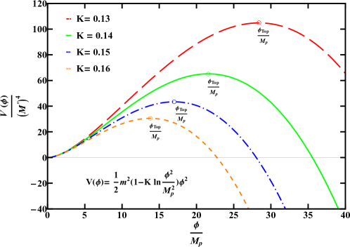
Figure 2: The plot of potential versus $\frac{\phi}{M_{P}}$ for quadratic chaotic model with corrected mass $V(\phi)=\frac{1}{2}m^{2}\left(1-\text{K}\ln\frac{\phi^{2}}{M_{P}^{2}}\right)\phi^{2}$ for different values of K : K=0.13 (large dashed red), K=0.14 (solid green), K=0.15 (dot-dashed blue), K=0.16 (small dashed orange). The small circle on each curve signifies the maxima of potential in each case and the corresponding field value at maxima is $\frac{\phi_{Top}}{M_{P}}$.

We will start our discussion with various field domains [35] within which inflationary phenomena may occur for above potential. It is evident that the above-mentioned potential eq. (28) does not exhibit positive definiteness for all values of the field (${\phi}$). The value of this potential becomes negative after a specific point

$$\frac{\phi_{V=0}}{M_{P}}=\sqrt{e^{\frac{1}{\text{K}}}}.$$ (29)

The model can only be defined within a specific regime i.e., $\phi<\phi_{V=0}$. On the contrary, the highest point of the potential function, where $V^{\prime}=0$ (or can say $\epsilon=0)$, corresponds to field value given as:

$$\frac{\phi_{V^{\prime}=0}}{M_{P}}=\frac{\phi_{Top}}{M_{P}}=\sqrt{e^{\frac{1-\text{K}}{\text{K}}}},$$ (30)

The model has a sense provided the correction term doesn’t have its dominance on the potential, hence the suitable regime is $\phi<\phi_{Top}<\phi_{V=0}$. The potential versus $\frac{\phi}{M_{P}}$ plot for four different values of K is depicted in figure 2. From figure 2 it can be seen that each K has specific viable regime in which the model is defined and have a sense and we will be working in these regions only.
Now moving further, the slow-roll parameters for this potential can be given as

$$\epsilon=2M_{P}^{2}\left(\frac{1-\text{K}\left(1+\ln\frac{\phi^{2}}{M_{P}^{2}}\right)}{\phi(1-\text{K}\ln\frac{\phi^{2}}{M_{P}^{2}}}\right)^{2},$$ (31)

$$\eta=\frac{2M_{P}^{2}\left(-3\text{K}+1-\text{K}\ln\frac{\phi^{2}}{M_{P}^{2}}\right)}{\phi^{2}\left(1-\text{K}\ln\frac{\phi^{2}}{M_{P}^{2}}\right)}.$$ (32)

After substituting the values of $\epsilon$ eq. (31) and $\eta$ eq. (32) in eq. (8), we can write scalar spectral index as

$$n_{s}=\frac{-4\left(2-3\text{K}+3\text{K}^{2}\right)+\frac{\phi^{2}}{M_{P}^{2}}-2\text{K}\left(-8+6\text{K}+\frac{\phi^{2}}{M_{P}^{2}}\right)\ln\frac{\phi^{2}}{M_{P}^{2}}+\text{K}^{2}\left(-8+\frac{\phi^{2}}{M_{P}^{2}}\right)\ln\left[\frac{\phi^{2}}{M_{P}^{2}}\right]^{2}}{\frac{\phi^{2}}{M_{P}^{2}}\left(-1+\text{K}\ln\frac{\phi^{2}}{M_{P}^{2}}\right)^{2}}.$$ (33)

The Hubble parameter during the crossing of Hubble radius by scale $k$ can be written as

$$H_{k}^{2}=\frac{1}{M_{P}^{2}}\left(\frac{V_{k}}{3-\epsilon_{k}}\right)=\left(\frac{\frac{1}{2}m^{2}\left(1-\text{K}\ln\frac{\phi_{k}^{2}}{M_{P}^{2}}\right)\frac{\phi_{k}^{2}}{M_{P}^{2}}}{3-2M_{P}^{2}\left(\frac{1-\text{K}\left(1+\ln\frac{\phi^{2}}{M_{P}^{2}}\right)}{\phi\left(1-\text{K}\ln\frac{\phi^{2}}{M_{P}^{2}}\right)}\right)^{2}}\right).$$ (34)

Using the condition $\epsilon=1$ defining end of inflation, we have obtained $\frac{\phi_{\text{end}}}{M_{P}}$ for different values of K. The remaining number of e-folds persist subsequent to crossing of hubble radius by $k_{*}$ till the termination of inflationary epoch can be given as

$$\text{$\Delta$}N_{*}\simeq\frac{1}{M_{P}^{2}}\int_{\phi_{\text{end}}}^{\phi_{*}}\frac{V}{V^{\prime}}\,d\phi_{*}=\frac{1}{2M_{P}^{2}}\int_{\phi_{\text{end}}}^{\phi_{*}}\frac{\left(1-\text{K {ln}}\frac{\phi^{2}}{M_{P}^{2}}\right)\phi}{1-\text{K}\left(1+\text{ln}\frac{\phi^{2}}{M_{P}^{2}}\right)}\,d\phi.$$ (35)

Defining $\frac{\phi_{*}}{M_{P}}=x$. The spectral index $n_{s}$ eq. (33), at $\phi=\phi_{*}$ in terms of $x$ will have the form

$$n_{s}=\frac{-4\left(2-3\text{K}+3\text{K}^{2}\right)+x^{2}-2\text{K}\left(-8+6\text{K}+x^{2}\right)\ln x^{2}+\text{K}^{2}\left(-8+x^{2}\right)\ln\left[x^{2}\right]^{2}}{x^{2}\left(-1+\text{K}\ln x^{2}\right)^{2}}.$$ (36)

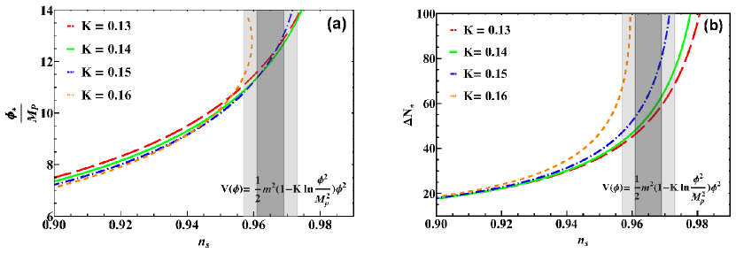
Figure 3: The plots of (a) $\frac{\phi_{*}}{M_{P}}$ and (b) $\text{$\Delta$N}_{*}$ versus $n_{s}$ for quadratic chaotic model with corrected mass $V(\phi)=\frac{1}{2}m^{2}\left(1-\text{K}\ln\frac{\phi^{2}}{M_{P}^{2}}\right)\phi^{2}$ for different values of K. The shaded regions and color codings are same as in figure 1 and 2 respectively.

;

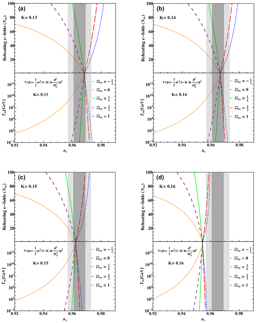
Figure 4: The plots for $T_{\text{re}}$ and $N_{\text{re}}$ versus spectral index ($n_{s}$) for quadratic chaotic model with corrected mass $V(\phi)=\frac{1}{2}m^{2}\left(1-\text{K}\ln\frac{\phi^{2}}{M_{P}^{2}}\right)\phi^{2}$ for different K and $\overline{\omega}_{\text{re}}$ values. The shaded regions and color codings are same as in figure 1

The variation of $\frac{\phi_{*}}{M_{P}}$ and $\text{$\Delta$N}_{*}$ with $n_{s}$ using eq. (36) and eq. (35) for 4 different values of K are shown in figure 3a and 3b respectively. Further in this model, we can write the tensor - to - scalar ratio and $H_{*}$ as

$$r=32\left(\frac{1-\text{K}\left(1+\ln x^{2}\right)}{x\left(1-\text{K}\ln x^{2}\right)}\right)^{2}.$$ (37)

$$H_{*}=4\pi M_{P}\sqrt{A_{s}}\left(\frac{1-\text{K}\left(1+\ln x^{2}\right)}{x\left(1-\text{K}\ln x^{2}\right)}\right).$$ (38)

Defining $\frac{\phi_{\text{end}}}{M_{P}}=y$. The relation of field $\phi$ and $H$, and the condition for termination of inflation, along with eq. (38) gives expression for $V_{\text{end}}$ in terms of $x$ and $y$ as

$$V_{\text{end}}(\phi)=\frac{1}{2}m^{2}\left(1-\text{K}\ln\left(\frac{\phi_{\text{end}}^{2}}{M_{P}^{2}}\right)\right)\phi_{\text{end}}^{2}\\ \\ \text{ }=\frac{3H_{*}^{2}M_{P}^{2}\left(1-\text{K}\ln y^{2}\right)y^{2}}{x^{2}\left(1-\text{K}\ln x^{2}\right)}\text{ }.$$ (39)

Now, the expressions for $\Delta$$N_{*}$, $r$, $H_{*}$ and $V_{\text{end}}$ as function of $n_{s\text{ }}$ can be obtained by putting the value of $x$ from eq. (36) and the value of y obtained using the condition for termination of inflation ($\epsilon=1$) in eqs. (35), (37), (38) and (39), and then these expressions along with eqs. (18) and(19) gives number of reheating e-folds $N_{\text{re}}$ and reheating temperature $T_{\text{re}}$. The $N_{\text{re}}$ and $T_{\text{re}}$ versus $n_{s}$ plots, along with Planck-2018 bounds, for 4 different K values for this model are presented graphically in figure 4.
By demanding $T_{\text{re}}>100$ GeV for production of weak-scale dark matter and solving eqs. (18) and (36), the bounds on $n_{s}$ are obtained and are reflected on eq. (35) and eq. (37) to obtain bounds on $\Delta$$N_{*}$ and r. All the obtained bounds for various choices of K are shown in table (2). The r versus $n_{s}$ plots, along with Planck-2018 bounds, for a range of K values are presented graphically in figure 5. The figure 5 shows that the tensor- to scalar ratio is greater than the viable range ($r<0.06)$ for ${\text{K}}\leq 0.13$ while for ${\text{K}}>0.16$ the $n_{s}$ value is outside Planck’s 2018 bound for any choice of $\overline{\omega}_{\text{re}}$. The value $\text{K}=0$ gives us the normal quadratic chaotic potential. The allowed range of K satisfying Planck’s 2018 constraints on both $n_{s}$ and r for this model is found to be ($0.13<{\text{K}}\leq 0.16$). Individually, the range of $\overline{\omega}_{\text{re}}$ for which our obtained data is compatible with Planck-2018 $2\sigma$ bounds on $n_{s}$ and the combined BICEP2/Keck and Planck’s bound on r, i.e. ($r<0.06)$ gives ($0.352<\overline{\omega}_{\text{re}}\leq 1$) for K=0.14 and ($0.009\leq\overline{\omega}_{\text{re}}\leq 1$) for K=0.15. For ${\text{K}}\leq 0.13$, there is no compatibility with data for any value of $\overline{\omega}_{\text{re}}$ taken and K=0.16 is compatible with data for only $\overline{\omega}_{\text{re}}$=1 . Similarly, the $1\sigma$ bound on $n_{s}$ and $r<0.06$ gives ($0.352<\overline{\omega}_{\text{re}}\leq 0.640$) for K=0.14 and ($0.212\leq\overline{\omega}_{\text{re}}\leq 1$) for K=0.15 while K=0.13 and K=0.16 are completely outside the combined $1\sigma$ and r bounds.

Table 2: The permissible range for $n_{s}$, $\Delta N_{*}$ and $r$ for different K values for modified Quadratic Chaotic inflation by demanding $T_{re}\geq 100GeV$

K = $0.13$	Average Equation of state	$n_{s}$	$\Delta N_{*}$	$r$
	$-\frac{1}{3}\leq\overline{\omega}_{re}\leq 0$	$0.932\leq n_{s}\leq 0.962$	$26.07\leq\Delta N_{*}\leq 47.03$	$0.195\geq r\geq 0.096$
	$0\leq\overline{\omega}_{re}\leq\frac{1}{6}$	$0.962\leq n_{s}\leq 0.966$	$47.03\leq\Delta N_{*}\leq 52.95$	$0.096\geq r\geq 0.083$
	$\frac{1}{6}\leq\overline{\omega}_{re}\leq\frac{2}{3}$	$0.966\leq n_{s}\leq 0.971$	$52.95\leq\Delta N_{*}\leq 63.56$	$0.083\geq r\geq 0.066$
	$\frac{2}{3}\leq\overline{\omega}_{re}\leq 1$	$0.971\leq n_{s}\leq 0.973$	$63.56\leq\Delta N_{*}\leq 67.68$	$0.066\geq r\geq 0.060$
4 K = $0.14$	$-\frac{1}{3}\leq\overline{\omega}_{re}\leq 0$	$0.931\leq n_{s}\leq 0.960$	$26.02\leq\Delta N_{*}\leq 46.94$	$0.175\geq r\geq 0.080$
	$0\leq\overline{\omega}_{re}\leq\frac{1}{6}$	$0.960\leq n_{s}\leq 0.964$	$46.94\leq\Delta N_{*}\leq 52.86$	$0.080\geq r\geq 0.068$
	$\frac{1}{6}\leq\overline{\omega}_{re}\leq\frac{2}{3}$	$0.964\leq n_{s}\leq 0.969$	$52.86\leq\Delta N_{*}\leq 63.46$	$0.068\geq r\geq 0.052$
	$\frac{2}{3}\leq\overline{\omega}_{re}\leq 1$	$0.969\leq n_{s}\leq 0.971$	$63.46\leq\Delta N_{*}\leq 67.56$	$0.052\geq r\geq 0.047$
4 K = $0.15$	$-\frac{1}{3}\leq\overline{\omega}_{re}\leq 0$	$0.929\leq n_{s}\leq 0.957$	$25.95\leq\Delta N_{*}\leq 46.84$	$0.152\geq r\geq 0.063$
	$0\leq\overline{\omega}_{re}\leq\frac{1}{6}$	$0.957\leq n_{s}\leq 0.960$	$46.84\leq\Delta N_{*}\leq 52.74$	$0.063\geq r\geq 0.052$
	$\frac{1}{6}\leq\overline{\omega}_{re}\leq\frac{2}{3}$	$0.960\leq n_{s}\leq 0.965$	$52.74\leq\Delta N_{*}\leq 63.31$	$0.052\geq r\geq 0.037$
	$\frac{2}{3}\leq\overline{\omega}_{re}\leq 1$	$0.965\leq n_{s}\leq 0.966$	$63.31\leq\Delta N_{*}\leq 67.40$	$0.037\geq r\geq 0.033$
4 K = $0.16$	$-\frac{1}{3}\leq\overline{\omega}_{re}\leq 0$	$0.925\leq n_{s}\leq 0.950$	$25.88\leq\Delta N_{*}\leq 46.71$	$0.129\geq r\geq 0.044$
	$0\leq\overline{\omega}_{re}\leq\frac{1}{6}$	$0.950\leq n_{s}\leq 0.953$	$46.71\leq\Delta N_{*}\leq 52.60$	$0.044\geq r\geq 0.034$
	$\frac{1}{6}\leq\overline{\omega}_{re}\leq\frac{2}{3}$	$0.953\leq n_{s}\leq 0.956$	$52.60\leq\Delta N_{*}\leq 63.11$	$0.034\geq r\geq 0.022$
	$\frac{2}{3}\leq\overline{\omega}_{re}\leq 1$	$0.956\leq n_{s}\leq 0.957$	$63.11\leq\Delta N_{*}\leq 67.18$	$0.022\geq r\geq 0.019$

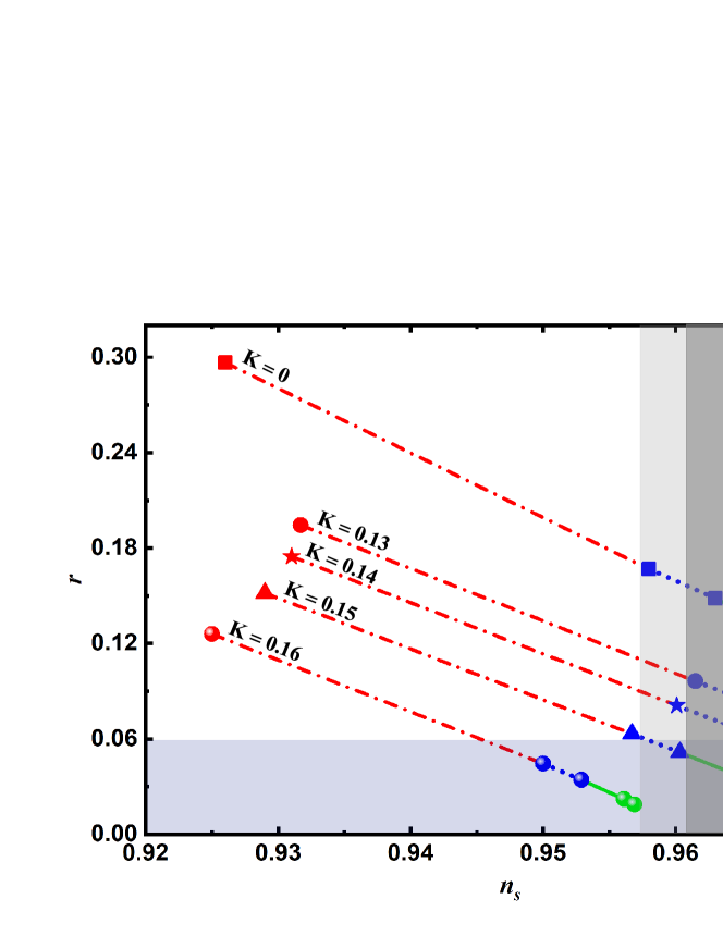
Figure 5: The r versus $n_{s}$ plot for range of K value with different $\overline{\omega}_{\text{re}}$: $-\frac{1}{3}\leq\overline{\omega}_{re}<0$(dot-dashed red), $0\leq\overline{\omega}_{re}\leq\frac{1}{6}$(dotted blue), $\frac{1}{6}<\overline{\omega}_{re}\leq 1$(solid green). The region with bluish shade corresponds to ($r<0.06$), the combined BICEP2/Keck and Planck’s bound [59, 16] on r while the gray regions are same as figure 1.

Table 3: The range of $T_{re}$ and $N_{re}$ for potential $V(\phi)=\frac{1}{2}m^{2}\left(1-\text{K}\ln\frac{\phi^{2}}{M_{P}^{2}}\right)\phi^{2}$ which shows compatibility with Planck’s 2018 1$\sigma$ bound on $n_{s}$.

	K $=0.13$		K $=0.14$		K $=0.15$
	$T_{re}$(GeV)	$N_{re}$	$T_{re}$(GeV)	$N_{re}$	$T_{re}$(GeV)	$N_{re}$
$\overline{\omega}_{re}=-\frac{1}{3}$	$T_{re}\geq 5.51\times 10^{10}$	$N_{re}\leq 22.09$	$T_{re}\geq 3.58\times 10^{11}$	$N_{re}\leq 18.30$	$T_{re}\geq 1.38\times 10^{14}$	$N_{re}\leq 5.86$
$\overline{\omega}_{re}=0$	$T_{re}\geq 14.06$	$N_{re}\leq 44.18$	$T_{re}\geq 4.04\times 10^{3}$	$N_{re}\leq 36.60$	$T_{re}\geq 3.92\times 10^{11}$	$N_{re}\leq 11.72$
$\overline{\omega}_{re}=\frac{1}{6}$	$10^{16}\geq T_{re}\geq 10^{-2}$	$N_{re}\leq 88.36$	$10^{16}\geq T_{re}\geq 10^{-2}$	$N_{re}\leq 73.21$	$T_{re}\geq 3.19\times 10^{6}$	$N_{re}\leq 23.44$
$\overline{\omega}_{re}=\frac{2}{3}$	$T_{re}\geq 7.12\times 10^{11}$	$N_{re}\leq 6.67$	$T_{re}\geq 249.61$	$N_{re}\leq 23.95$	$10^{16}\geq T_{re}\geq 10^{-2}$	$N_{re}\leq 94.11$
$\overline{\omega}_{re}=1$	$T_{re}\geq 2.03\times 10^{13}$	$N_{re}\leq 3.35$	$T_{re}\geq 3.95\times 10^{7}$	$N_{re}\leq 11.97$	$10^{16}\geq T_{re}\geq 10^{-2}$	$N_{re}\leq 47.05$

We have also found the viable range of the reheat temperature and number of e-foldings for each case which shows compatibility with Planck’s 2018 1$\sigma$ bound on $n_{s}$ using figure 4 and the findings have been clearly presented in a tabular format in table 3. The table 3 shows that the curve corresponding to $\overline{\omega}_{\text{re}}=\frac{1}{6}$ for K=0.13 and 0.14 and the curves corresponding to ($\frac{2}{3}\leq\overline{\omega}_{\text{re}}\leq 1$) for K=0.15, give every possible value of reheating temperature ($10^{-2}$ GeV to $10^{16}$ GeV) while K=0.16 shows incompatibility with data for all $\overline{\omega}_{\text{re}}$ taken. The $n_{s}$ values for these $\overline{\omega}_{\text{re}}$ ranges are 0.966 and 0.964 for K=0.13 and 0.14 while it is (0.965 $<$ $n_{s}$ $\leq$ 0.966) for K=0.15 which sets limit on tensor to scalar ratio(r) and the obtained values of r are 0.083 and 0.068 for K=0.13 and 0.14 while it is (0.037 $\leq$ r $\leq$ 0.033) for K=0.15 and only the r values for K=0.15 are satisfying the condition ($r<0.06)$.

4 Discussion and conclusion

In this work, we have considered a modified form of quadratic chaotic inflation. Our primary goal is to study the reheating phase in light of Planck’s 2018 observations. For that, we have considered two parameters, namely duration of reheating $N_{\text{re}}$ and reheating temperature $T_{\text{re}}$ and obtained their variation as function of scalar spectral index $n_{\text{s}}$ by considering a suitable range of effective equation of state $\overline{\omega}_{\text{re}}$. By demanding $T_{\text{re}}>100$ GeV for production of weak-scale dark matter and allowing $\overline{\omega}_{\text{re}}$ to vary in the range ($-\frac{1}{3}\leq\overline{\omega}_{\text{re}}\leq 1$), we tried to find the permissible ranges for $n_{\text{s}}$, $\Delta N_{*}$ and tensor-to-scalar ratio(r) for our models.
We first restudied the simple quadratic chaotic inflation using the most recent Planck’s 2018 data and found that the condition $T_{\text{re}}$ $>$ 100 GeV gives ($-0.03\leq\overline{\omega}_{\text{re}}\leq 1$) for $n_{s}$ to lie inside Planck-2018 $2\sigma$ bounds while if we demand $n_{s}$ to lie within $1\sigma$ bounds than the allowed range of $\overline{\omega}_{\text{re}}$ is ($0.09\leq\overline{\omega}_{\text{re}}\leq 0.67$). Within these ranges of $\overline{\omega}_{\text{re}}$, r is greater than the combined BICEP2/Keck and Planck’s bound on r, i.e. ($r<0.06)$.
Since the normal quadratic chaotic potential is not favoring the observational data. We have considered a modified form of quadratic chaotic potential where a logarithmic correction containing a model parameter K is added to the mass term. We have found that for each value of model parameter K of the modified model, there is only a specific range of inflaton field $(\phi)$ within which the model is defined and the correction part is not dominant over the actual quadratic term of potential. We have constrained ourself to only those regions for our analysis. By imposing the reheating conditions on this model, we found that the constraints on $n_{\text{s}}$ and r are consistent with Planck’s 2018 data for only a particular range of K values and is found to be ($0.13<{\text{K}}\leq 0.16$), where each K value has a different range of $\overline{\omega}_{\text{re}}$ in which it is compatible with the data. The ranges of $\overline{\omega}_{\text{re}}$ for which our obtained data is compatible with Planck-2018 $2\sigma$ bounds on $n_{s}$ and the combined BICEP2/Keck and Planck’s bound on r, i.e. ($r<0.06)$ gives ($0.352<\overline{\omega}_{\text{re}}\leq 1$) for K=0.14 and ($0.009\leq\overline{\omega}_{\text{re}}\leq 1$) for K=0.15. For ${\text{K}}\leq 0.13$, there is no compatibility with data for any value of $\overline{\omega}_{\text{re}}$ taken and K=0.16 is compatible with data for only $\overline{\omega}_{\text{re}}$=1 . Similarly, the $1\sigma$ bound on $n_{s}$ and $r<0.06$ gives ($0.352<\overline{\omega}_{\text{re}}\leq 0.640$) for K=0.14 and ($0.212\leq\overline{\omega}_{\text{re}}\leq 1$) for K=0.15 while K=0.13 and K=0.16 are completely outside the combined $1\sigma$ and r bounds.
Also, from the plots showing the variation of $T_{\text{re}}$ with $n_{s}$, we have found that different values of K and $\overline{\omega}_{\text{re}}$ give different ranges of reheating temperature as compatible with Planck’s 1$\sigma$ bounds on $n_{\text{s}}$, but if we allow $T_{\text{re}}$ to vary over the whole range ( $10^{-2}$ GeV to $10^{16}$ GeV) , then $\overline{\omega}_{\text{re}}$ is restricted to ($0.047\leq\overline{\omega}_{\text{re}}\leq 0.391$) for K=0.13, ($0.087\leq\overline{\omega}_{\text{re}}\leq 0.559$) for K=0.14 and ($0.237\leq\overline{\omega}_{\text{re}}\leq 1$) for K=0.15 while K=0.16 shows incompatibility with Planck’s 2018 1$\sigma$ bounds on $n_{\text{s}}$ for all $\overline{\omega}_{\text{re}}$ taken.
To conclude, the reheating study shows that the values of K close to 0.15 are more favorable ones and the $\overline{\omega}_{\text{re}}$ range satisfying the observational data for K=0.15 suggests the possible production of Feebly Interacting Massive Particle(FIMP) and Weakly Interacting Massive Particle(WIMP)-like dark matter particles [60, 61] and primordial black holes [62]. Elaborated study of possible particle production will be done in our future publications. The findings of the reheating study prove that even a small correction in mass term can help quadratic chaotic potential to favour Planck-2018 observations. Also, we have found that considering the reheating constraints, the average equation of state parameter $\overline{\omega}_{\text{re}}$ plays a vital role in defining the compatible range of reheating parameters, which effectively narrows the model’s viable parameter space and significantly increases the model’s accuracy.

References

- [1] Alan H. Guth “Inflationary universe: A possible solution to the horizon and flatness problems” In Physical Review D 23.2, 1981, pp. 347–356 DOI: 10.1103/PhysRevD.23.347
- [2] A.A. Starobinsky “A new type of isotropic cosmological models without singularity” In Physics Letters B 91.1, 1980, pp. 99–102 DOI: 10.1016/0370-2693(80)90670-X
- [3] A.D. Linde “A new inflationary universe scenario: A possible solution of the horizon, flatness, homogeneity, isotropy and primordial monopole problems” In Physics Letters B 108.6, 1982, pp. 389–393 DOI: 10.1016/0370-2693(82)91219-9
- [4] A.D. Linde “Chaotic inflation” In Physics Letters B 129.3-4, 1983, pp. 177–181 DOI: 10.1016/0370-2693(83)90837-7
- [5] Antonio Riotto “Inflation and the Theory of Cosmological Perturbations”, 2002 DOI: 10.48550/ARXIV.HEP-PH/0210162
- [6] V.. Mukhanov and G.. Chibisov “Quantum fluctuations and a nonsingular universe” ADS Bibcode: 1981ZhPmR..33..549M In ZhETF Pisma Redaktsiiu 33, 1981, pp. 549–553
- [7] A.A. Starobinsky “Dynamics of phase transition in the new inflationary universe scenario and generation of perturbations” In Physics Letters B 117.3-4, 1982, pp. 175–178 DOI: 10.1016/0370-2693(82)90541-X
- [8] Alan H. Guth and So-Young Pi “Quantum mechanics of the scalar field in the new inflationary universe” In Physical Review D 32.8, 1985, pp. 1899–1920 DOI: 10.1103/PhysRevD.32.1899
- [9] G.. Smoot et al. “Structure in the COBE Differential Microwave Radiometer First-Year Maps” ADS Bibcode: 1992ApJ…396L…1S In The Astrophysical Journal 396, 1992, pp. L1 DOI: 10.1086/186504
- [10] J. Dunkley et al. “FIVE-YEAR WILKINSON MICROWAVE ANISOTROPY PROBE OBSERVATIONS: LIKELIHOODS AND PARAMETERS FROM THE WMAP DATA” In The Astrophysical Journal Supplement Series 180.2, 2009, pp. 306–329 DOI: 10.1088/0067-0049/180/2/306
- [11] E. Komatsu et al. “SEVEN-YEAR WILKINSON MICROWAVE ANISOTROPY PROBE ( WMAP ) OBSERVATIONS: COSMOLOGICAL INTERPRETATION” In The Astrophysical Journal Supplement Series 192.2, 2011, pp. 18 DOI: 10.1088/0067-0049/192/2/18
- [12] P… Ade et al. “Planck 2013 results. XVI. Cosmological parameters” In Astronomy & Astrophysics 571, 2014, pp. A16 DOI: 10.1051/0004-6361/201321591
- [13] P… Ade et al. “Planck 2013 results. XXII. Constraints on inflation” In Astronomy & Astrophysics 571, 2014, pp. A22 DOI: 10.1051/0004-6361/201321569
- [14] P… Ade et al. “Planck 2015 results: XIII. Cosmological parameters” In Astronomy & Astrophysics 594, 2016, pp. A13 DOI: 10.1051/0004-6361/201525830
- [15] P… Ade et al. “Planck 2015 results: XX. Constraints on inflation” In Astronomy & Astrophysics 594, 2016, pp. A20 DOI: 10.1051/0004-6361/201525898
- [16] N. Aghanim et al. “Planck 2018 results: VI. Cosmological parameters” In Astronomy & Astrophysics 641, 2020, pp. A6 DOI: 10.1051/0004-6361/201833910
- [17] Y. Akrami et al. “Planck 2018 results: X. Constraints on inflation” In Astronomy & Astrophysics 641, 2020, pp. A10 DOI: 10.1051/0004-6361/201833887
- [18] Michael S. Turner “Coherent scalar-field oscillations in an expanding universe” In Physical Review D 28.6, 1983, pp. 1243–1247 DOI: 10.1103/PhysRevD.28.1243
- [19] Jennie H. Traschen and Robert H. Brandenberger “Particle production during out-of-equilibrium phase transitions” In Physical Review D 42.8, 1990, pp. 2491–2504 DOI: 10.1103/PhysRevD.42.2491
- [20] Andreas Albrecht, Paul J. Steinhardt, Michael S. Turner and Frank Wilczek “Reheating an Inflationary Universe” In Physical Review Letters 48.20, 1982, pp. 1437–1440 DOI: 10.1103/PhysRevLett.48.1437
- [21] Lev Kofman, Andrei Linde and Alexei A. Starobinsky “Reheating after Inflation” In Physical Review Letters 73.24, 1994, pp. 3195–3198 DOI: 10.1103/PhysRevLett.73.3195
- [22] Lev Kofman, Andrei Linde and Alexei A. Starobinsky “Towards the theory of reheating after inflation” In Physical Review D 56.6, 1997, pp. 3258–3295 DOI: 10.1103/PhysRevD.56.3258
- [23] Marco Drewes and Jin U Kang “The kinematics of cosmic reheating” In Nuclear Physics B 875.2, 2013, pp. 315–350 DOI: 10.1016/j.nuclphysb.2013.07.009
- [24] Rouzbeh Allahverdi, Robert Brandenberger, Francis-Yan Cyr-Racine and Anupam Mazumdar “Reheating in Inflationary Cosmology: Theory and Applications” In Annual Review of Nuclear and Particle Science 60.1, 2010, pp. 27–51 DOI: 10.1146/annurev.nucl.012809.104511
- [25] Jérôme Martin, Christophe Ringeval and Vincent Vennin “Observing Inflationary Reheating” In Physical Review Letters 114.8, 2015, pp. 081303 DOI: 10.1103/PhysRevLett.114.081303
- [26] Jérôme Martin and Christophe Ringeval “First CMB constraints on the inflationary reheating temperature” In Physical Review D 82.2, 2010, pp. 023511 DOI: 10.1103/PhysRevD.82.023511
- [27] Liang Dai, Marc Kamionkowski and Junpu Wang “Reheating Constraints to Inflationary Models” In Physical Review Letters 113.4, 2014, pp. 041302 DOI: 10.1103/PhysRevLett.113.041302
- [28] Jérôme Martin and Christophe Ringeval “Inflation after WMAP3: confronting the slow-roll and exact power spectra with CMB data” In Journal of Cosmology and Astroparticle Physics 2006.08, 2006, pp. 009–009 DOI: 10.1088/1475-7516/2006/08/009
- [29] Peter Adshead, Richard Easther, Jonathan Pritchard and Abraham Loeb “Inflation and the scale dependent spectral index: prospects and strategies” In Journal of Cosmology and Astroparticle Physics 2011.02, 2011, pp. 021–021 DOI: 10.1088/1475-7516/2011/02/021
- [30] Jakub Mielczarek “Reheating temperature from the CMB” In Physical Review D 83.2, 2011, pp. 023502 DOI: 10.1103/PhysRevD.83.023502
- [31] Jessica L. Cook, Emanuela Dimastrogiovanni, Damien A. Easson and Lawrence M. Krauss “Reheating predictions in single field inflation” In Journal of Cosmology and Astroparticle Physics 2015.04, 2015, pp. 047–047 DOI: 10.1088/1475-7516/2015/04/047
- [32] Gary Steigman “Primordial Nucleosynthesis in the Precision Cosmology Era” In Annual Review of Nuclear and Particle Science 57.1, 2007, pp. 463–491 DOI: 10.1146/annurev.nucl.56.080805.140437
- [33] Scott Dodelson and Lam Hui “Horizon Ratio Bound for Inflationary Fluctuations” In Physical Review Letters 91.13 American Physical Society (APS), 2003 DOI: 10.1103/physrevlett.91.131301
- [34] Andrew R. Liddle and Samuel M. Leach “How long before the end of inflation were observable perturbations produced?” In Physical Review D 68.10 American Physical Society (APS), 2003 DOI: 10.1103/physrevd.68.103503
- [35] Jerome Martin, Christophe Ringeval and Vincent Vennin “Encyclopaedia Inflationaris” arXiv:1303.3787 [astro-ph, physics:gr-qc, physics:hep-ph, physics:hep-th], 2013 DOI: 10.48550/arXiv.1303.3787
- [36] V. Şenoğuz and Qaisar Shafi “Chaotic inflation, radiative corrections and precision cosmology” In Physics Letters B 668.1, 2008, pp. 6–10 DOI: 10.1016/j.physletb.2008.08.017
- [37] Kari Enqvist and Mindaugas Karčiauskas “Does Planck really rule out monomial inflation?” In Journal of Cosmology and Astroparticle Physics 2014.02, 2014, pp. 034–034 DOI: 10.1088/1475-7516/2014/02/034
- [38] Guillermo Ballesteros and Carlos Tamarit “Radiative plateau inflation” In Journal of High Energy Physics 2016.2, 2016, pp. 153 DOI: 10.1007/JHEP02(2016)153
- [39] Kazunori Nakayama, Fuminobu Takahashi and Tsutomu T. Yanagida “Polynomial chaotic inflation in the Planck era” In Physics Letters B 725.1-3, 2013, pp. 111–114 DOI: 10.1016/j.physletb.2013.06.050
- [40] Kazunori Nakayama and Fuminobu Takahashi “Running kinetic inflation” In Journal of Cosmology and Astroparticle Physics 2010.11, 2010, pp. 009–009 DOI: 10.1088/1475-7516/2010/11/009
- [41] Constantinos Pallis “Kinetically modified nonminimal chaotic inflation” In Physical Review D 91.12, 2015, pp. 123508 DOI: 10.1103/PhysRevD.91.123508
- [42] Kristjan Kannike et al. “Dynamically induced Planck scale and inflation” In Journal of High Energy Physics 2015.5, 2015, pp. 65 DOI: 10.1007/JHEP05(2015)065
- [43] Lotfi Boubekeur, Elena Giusarma, Olga Mena and Héctor Ramírez “Do current data prefer a nonminimally coupled inflaton?” In Physical Review D 91.10, 2015, pp. 103004 DOI: 10.1103/PhysRevD.91.103004
- [44] Luca Marzola and Antonio Racioppi “Minimal but non-minimal inflation and electroweak symmetry breaking” In Journal of Cosmology and Astroparticle Physics 2016.10, 2016, pp. 010–010 DOI: 10.1088/1475-7516/2016/10/010
- [45] Antonio Racioppi “New universal attractor in nonminimally coupled gravity: Linear inflation” In Physical Review D 97.12, 2018, pp. 123514 DOI: 10.1103/PhysRevD.97.123514
- [46] Shinta Kasuya and Mayuko Taira “Quadratic chaotic inflation with a logarithmic-corrected mass” In Physical Review D 98.12, 2018, pp. 123515 DOI: 10.1103/PhysRevD.98.123515
- [47] Debasish Borah, Dibyendu Nanda and Abhijit Kumar Saha “Common origin of modified chaotic inflation, nonthermal dark matter, and Dirac neutrino mass” In Phys. Rev. D 101.7, 2020, pp. 075006 DOI: 10.1103/PhysRevD.101.075006
- [48] Anish Ghoshal, Nobuchika Okada and Arnab Paul “eV Hubble scale inflation with a radiative plateau: Very light inflaton, reheating, and dark matter in B-L extensions” In Phys. Rev. D 106.9, 2022, pp. 095021 DOI: 10.1103/PhysRevD.106.095021
- [49] Rajesh Goswami and Urjit A. Yajnik “Reconciling low multipole anomalies and reheating in single field inflationary models” In Journal of Cosmology and Astroparticle Physics 2018.10, 2018, pp. 018–018 DOI: 10.1088/1475-7516/2018/10/018
- [50] Rajesh Goswami and Urjit A. Yajnik “Reheating constraints to modulus mass for single field inflationary models” In Nuclear Physics B 960, 2020, pp. 115211 DOI: 10.1016/j.nuclphysb.2020.115211
- [51] Debaprasad Maity and Pankaj Saha “Minimal plateau inflationary cosmologies and constraints from reheating” In Class. Quant. Grav. 36, 2019, pp. 045010 DOI: 10.1088/1361-6382/ab0038
- [52] Manuel Drees and Yong Xu “Small field polynomial inflation: reheating, radiative stability and lower bound” In JCAP 09, 2021, pp. 012 DOI: 10.1088/1475-7516/2021/09/012
- [53] Jerome Martin “Inflation and Precision Cosmology”, 2003 DOI: 10.48550/ARXIV.ASTRO-PH/0312492
- [54] D. Boyanovsky, H.. Vega, R. Holman and J… Salgado “Preheating and Reheating in Inflationary Cosmology: a pedagogical survey”, 1996 DOI: 10.48550/ARXIV.ASTRO-PH/9609007
- [55] Lev Kofman “Reheating and Preheating after Inflation”, 1998 DOI: 10.48550/ARXIV.HEP-PH/9802285
- [56] Gary Felder, Lev Kofman and Andrei Linde “Instant Preheating”, 1998 DOI: 10.48550/ARXIV.HEP-PH/9812289
- [57] Gian Francesco Giudice, Igor I Tkachev and Antonio Riotto “The cosmological moduli problem and preheating” In Journal of High Energy Physics 2001.06, 2001, pp. 020–020 DOI: 10.1088/1126-6708/2001/06/020
- [58] Mariel Desroche, Gary N. Felder, Jan M. Kratochvil and Andrei Linde “Preheating in new inflation” In Physical Review D 71.10, 2005, pp. 103516 DOI: 10.1103/PhysRevD.71.103516
- [59] P… Ade et al. “Constraints on Primordial Gravitational Waves Using , WMAP, and New BICEP2/ Observations through the 2015 Season” In Phys. Rev. Lett. 121 American Physical Society, 2018, pp. 221301 DOI: 10.1103/PhysRevLett.121.221301
- [60] MD Riajul Haque, Debaprasad Maity and Rajesh Mondal “WIMPs, FIMPs, and Inflaton phenomenology via reheating, CMB and ” In Journal of High Energy Physics 2023.9 Springer Berlin Heidelberg, 2023, pp. 12 DOI: 10.1007/JHEP09(2023)012
- [61] Md Riajul Haque and Debaprasad Maity “Gravitational dark matter: Free streaming and phase space distribution” In Physical Review D 106.2, 2022, pp. 023506 DOI: 10.1103/PhysRevD.106.023506
- [62] Tomohiro Harada, Chul-Moon Yoo and Kazunori Kohri “Threshold of primordial black hole formation” [Erratum: Phys.Rev.D 89, 029903 (2014)] In Phys. Rev. D 88.8, 2013, pp. 084051 DOI: 10.1103/PhysRevD.88.084051