Real-Time Motion Planning for In-Hand Manipulation with a Multi-Fingered Hand

Abstract

Dexterous manipulation of objects once held in hand remains a challenge. Such skills are, however, necessary for robotics to move beyond gripper-based manipulation and use all the dexterity offered by anthropomorphic robotic hands. One major challenge when manipulating an object within the hand is that fingers must move around the object while avoiding collision with other fingers or the object. Such collision-free paths must be computed in real-time, as the smallest deviation from the original plan can easily lead to collisions. We present a real-time approach to computing collision-free paths in a high-dimensional space. To guide the exploration, we learn an explicit representation of the free space, retrievable in real-time. We further combine this representation with closed-loop control via dynamical systems and sampling-based motion planning and show that the combination increases performance compared to alternatives, offering efficient search of feasible paths and real-time obstacle avoidance in a multi-fingered robotic hand.

I Introduction

In-hand manipulation, that is, the ability to manipulate objects once securely grasped by fingers, is essential to expand the range of manipulation tasks robots can perform. In-hand manipulation makes use of the full dexterity of high degrees of freedom robotic hands and is hence particularly well suited for multi-fingered hands. Moving an object in hand can be decomposed into a sequence of grasps by subgroups of fingers, whereby the object is swapped from one group of fingers to another. By so doing, the fingers modify the pose of the manipulated object until the object adopts the final desired pose [koshiba2011regrasp]. To induce the desired dynamics to the object requires various techniques well studied in the literature [mousavi2013new]. One can either slide the object alongside the fingers [paolini2014data], rotate the object in-between two or more fingers [4], or perform a combination of those motions [wan2019regrasp].

Figure 2: Examples of a successful (first row) and two failed regrasps of an elongated object held in hand. The task requires changing the initial two-finger pinch (leftmost picture in each row) to a four-finger pinch (rightmost picture in the first row). Collision with objects or across fingers can arise as the fingers move to reposition in the new grasp. Second row: the ring finger collides with the object as it moves around it, destabilizing it. Third row: the index and the middle fingers collide as the middle finger is closing on the object, leading the index to slip and let go of the object. Our approach that computes collision-free paths in real-time results in successful regrasp, as seen in the first row.

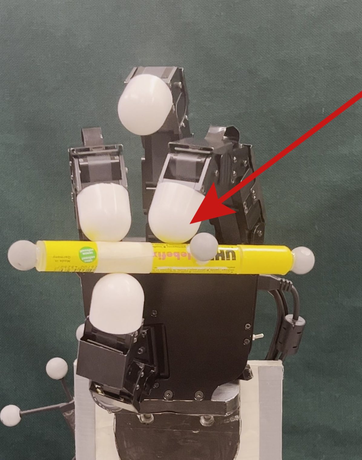
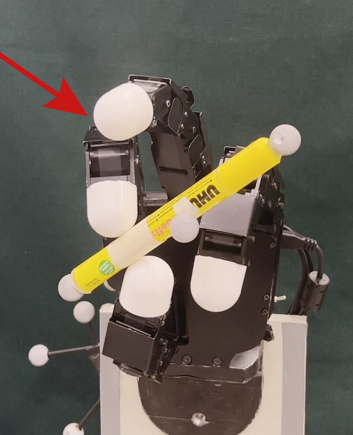
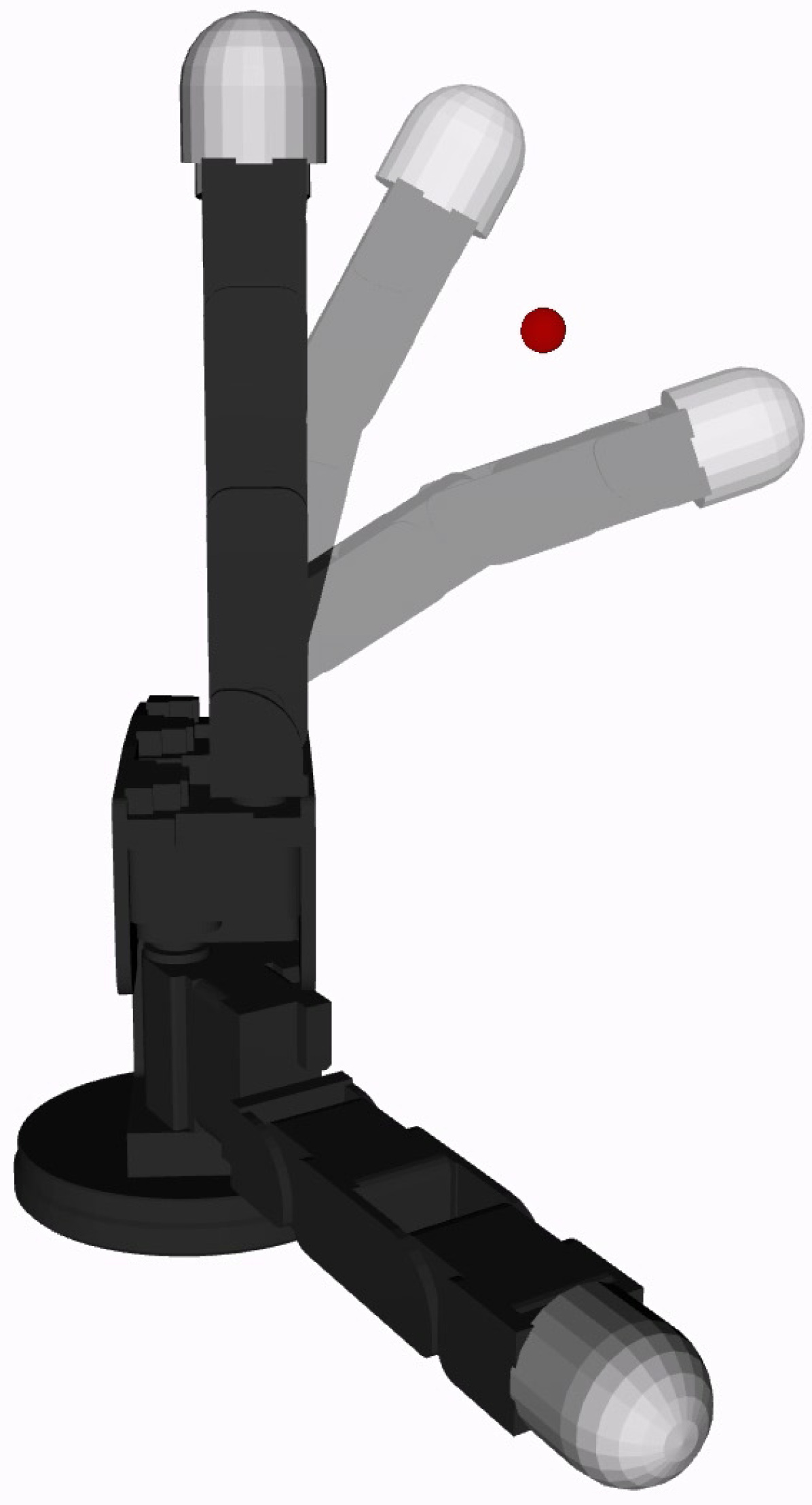
When the manipulation requires regrasp the object, as shown in Fig. 2, the fingers must be controlled to move around the object to reposition and form a new stable grasp. Different from traditional grasping, whereby fingers close on a static object supported by the environment [xue2008planning], grasping during in-hand manipulation is subject to more risk of dropping the object, as the object is transferred from one stable support to another one. With an object in hand, the available workspace for the fingers to move about is severely restricted. Hence, collisions are frequent. Fingers may collide with the object, as well as with one another, see examples in Fig. 2. This paper develops real-time collision-free planning approaches that ensure that the hand moves its fingers to the desired next configuration while maintaining the stability of the grasped object.

Despite numerous advances in the control of dexterous robotic hands [2, mason2018toward], the problem of performing online collision avoidance during in-hand manipulation remains a challenge. This paper offers an approach to explicitly model the free space within a hand using a set of learned distance functions, retrievable in real-time. These functions are then used in conjunction with dynamical systems control and sampling-based planning methods to speed up the search for a free path. This yields efficient and effective collision-free motion planning, and also contact-based in-hand manipulation for sliding. Our main contributions are in three aspects:

1. We propose a generalized implicit C-space representation for robot motion planning, considering both self-collision and collision with external objects.

2. We propose a fast and reactive motion planning approach that can generate collision-free motion paths in dynamic and cluttered environments in real-time.

3. We project the collision-free motion onto the isolines of the C-space for sliding motion planning.

4. We demonstrate the efficiency of our methods on a real multi-fingered robotic hand by adjusting the hand pose to avoid collision online. To our knowledge, this is the first work that tackles the real-time in-hand collision avoidance challenge for a multi-fingered robotic hand.

II Related Work

Collision detection is a fundamental aspect of collision-free motion planning, involving the computation of distances between robots and obstacles. The computational complexity of this task is exacerbated by the presence of numerous vertices in each robot and obstacle. A conventional approach involves performing forward kinematics to update the robot poses and computing the distances between geometric entities, such as through the use of the Flexible Collision Library (FCL) [PanFCL2012]. However, this process can be computationally intensive and impractical for real-time motion planning in dynamic environments with moving obstacles.

To improve the efficiency of collision detection, geometric primitives such as spheres or bounding boxes are often used to approximate the shapes of robots and obstacles []. However, these approximations can decrease the collision-free space and lead to the absence of feasible paths, particularly in in-hand manipulation tasks where finger motion is limited. To overcome this challenge, machine learning techniques have been developed to learn collision classifiers, such as the Support Vector Machine (SVM) [Sina2018unified] and Neural Network (NN) [Koptev2022NN]. By utilizing these methods, collision detection can be performed efficiently through parallel computing.

The planning of collision-free finger motions for in-hand manipulation can be either model-based or model-free. Model-based approaches often demand explicit models of the robotic hand and the manipulated object, such as geometric shapes, mass, inertia, and contact models. Then, the desired trajectories can be obtained by directly analyzing the relationships between the hand and the object. For example, Rohrdanz et al. [rohrdanz1997generating] generated regrasp motion by searching in the space of compatible regrasp operations, and considering the constraints and grasp quality. Xue et al. [xue2008planning] planned regrasp motion by first constructing a collision-free grasp database offline, then searching online by considering collision and kinematic feasibility. Shi et al. [shi2017dynamic] controlled the acceleration of the hand to create an inertial force on an object pinched by fingertips to slide. In both tasks, the object is pinched by fingertips, and the trajectories of both fingers and object are assumed collision-free.

Alternatively, optimization-based approaches can naturally ensure collision-free property by incorporating such requirements as problem constraints. These approaches have been successfully applied to generate grasping hand poses [5, 6] or a sequence of manipulation motions [mordatch2012contact]. [sundaralingam2018geometric] autonomously generate a sequence of finger placement for regrasping using alternating optimization. However, solving optimization problems suffers from high computational complexity and can hardly be used in real-time. Moreover, purely model-based approaches are sensitive to model inaccuracies and can hardly capture dynamically changing environments.

In contrast, model-free manipulation approaches usually do not require explicit models of the hand nor of the object, and, instead, use a policy to determine the best action at each state (e.g., configuration). Machine learning techniques can be used to learn a policy to control the hand for specific tasks [popov2017data], or to predict the occurrence of collision [Koptev2022NN]. OpenAI [1] combines reinforcement learning with a deep neural network to control a dexterous robotic hand to manipulate a Rubik’s cube. Google Brain [nagabandi2020deep] trained a deep neural network to enable a dexterous robotic hand to perform a variety of multiple dexterous manipulation motions. These approaches, however, require a long training time with large amounts of data. The policy needs to be retrained when manipulating novel objects.

Generating a collision-free trajectory for a finger in real-time becomes more challenging in a dynamic environment, for example, when the manipulated object or other fingers are also moving. Many works tried to tackle this challenge using an optimization-based approach. For example, iterative Linear Quadratic Regulator (iLQR) [todorov2005generalized] used for locally-optimal feedback control of nonlinear dynamical systems; or CHOMP [ratliff2009chomp] that minimizes the cost function by gradient descent. However, such approaches are prone to be trapped in local minima. Alternatively, STOMP [Kalakrishnan_STOMP_2011] considers the probabilities of feasible paths and exploits expectation-maximization to obtain a trajectory for the next step. Both CHOMP and STOMP use a spherical approximation of the robot body, and can hardly find a path for cluttered environments. Vannoy et al. [vannoy2008real] proposed an optimization-based approach that can be used for real-time motion planning for a high DoF robot; however, the convergence cannot be guaranteed. Moreover, all these optimization-based approaches suffer from high-computational costs. Hence, they cannot be applied to efficiently deal with a dynamically changing environment in real time.

Dynamical system (DS) based approaches have been successfully applied to tackle collision avoidance problems in Cartesian space for a point robot or the end-effector of a robotic arm [Mohammad2012DS_modulation]. A closed-form representation of the velocity field converged at the Cartesian target can be obtained by training a potential field [khatib1985real] by harmonic functions.

Given a geometric representation of the obstacle in space, the trained potential field can online adapt to the obstacle in space and guide the robot end-effector moving toward the target by following the collision-free velocity vector field. Such approaches are however often restricted to low-dimensional space. Huber et al. [huber2022avoiding] extended the state-of-the-art by constraining a flow in a volume around the object, in a closed-form representation. Such a flow guarantees convergence inside the volume, but global convergence can still not be guaranteed.

Sampling-based methods can help to alleviate the local minimum issues in these approaches. Such approaches are suitable for searching in high-dimensional spaces and can also be applied to online collision avoidance problems. One representative approach is the probabilistic roadmap (PRM) [kavraki1996probabilistic]. It constructs a roadmap in the configuration space (C-space) [lozano1990spatial]. The nodes of the map indicate states, connected by edges. A path that guides the robot from the initial to the goal state can be obtained by searching the map. Its variation, Lazy PRM [3], assumes the originally constructed PRM to be collision-free. It checks collisions online and updates the map at the same time to achieve fast trajectory queries. Variations of PRM include UOBPRM [yeh2012uobprm], which yields samples that are more uniformly distributed on C-obstacle surfaces. Another category of widely used approaches is proposed based on rapidly exploring random tree (RRT) [lavalle1998rapidly], which incrementally constructs a space-filling tree by randomly sampling toward unexplored space regions. Karaman et al. [karaman2011sampling] improved both RRT and PRM by proposing RRT* and PRM*, respectively. RRT* records each node’s distance to its parent and rewires the tree to increase smoothness. PRM* uses an adaptive radius to find neighbors and allows all sampled nodes to be connected within a certain distance. However, both algorithms suffer from dynamic environments. The roadmaps must be reconstructed once the obstacle moves. Recently, Naderi et al. [naderi2015rt] extends RRT* by introducing an online tree rewiring strategy, and proposes real-time RRT* for real-time path planning in dynamic environments. RRTX [otte2016rrtx] extends RRT to tackle the online obstacle avoidance problem. It adapts to the changing obstacle by rewiring the existing search graph in C-space and guarantees asymptotical optimality. To speed up the convergence rate of sampling-based methods, some combination methods are proposed to incorporate the potential field in sampling-based methods. qureshi2016potential proposed the P-RRT* by guiding the RRT* sampling by the potential field. OP-PRM [ye2022real] combines the potential field with PRM for effective sampling. However, these approaches only work in Cartesian space since the gradients in joint space are not available.

We consider a typical in-hand manipulation scenario, where a multi-fingered robotic hand grasps an object and tries to adapt to another grasp configuration. We aim to obtain a collision-free manipulation path for the hand to move from the initial state to the final state, and we assume the hand grasps the object stably in both states. We tackle this problem in three steps. First, in this section (Sec. III), we learn a model of the collision-free space by estimating a set of distance functions to separate the space region that is collision-free, from the region where collision exists among fingers, the palm, and the object. Next (Sec. IV), we sample inside the collision-free space model to obtain a collision-free motion path. To avoid unforeseen collisions during moving, we integrate the distance function with a reactive control system based on dynamical systems. Finally (Sec. V), we demonstrate the efficiency of our approach, which combines the reactive control system with sampling-based planning.

III NN-based C-space Representation

We first introduce the models used (Sec. III-A). Then, we explain our description of the collision-free C-space (Sec. III-B). The model of such a C-space is obtained through training both a self-collision model (Sec. III-C) and a hand-object collision model (Sec. III-D).

III-A Modelling of hand and object

III-A1 Hand model

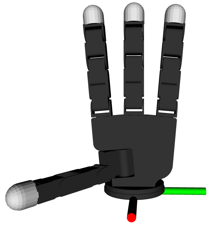
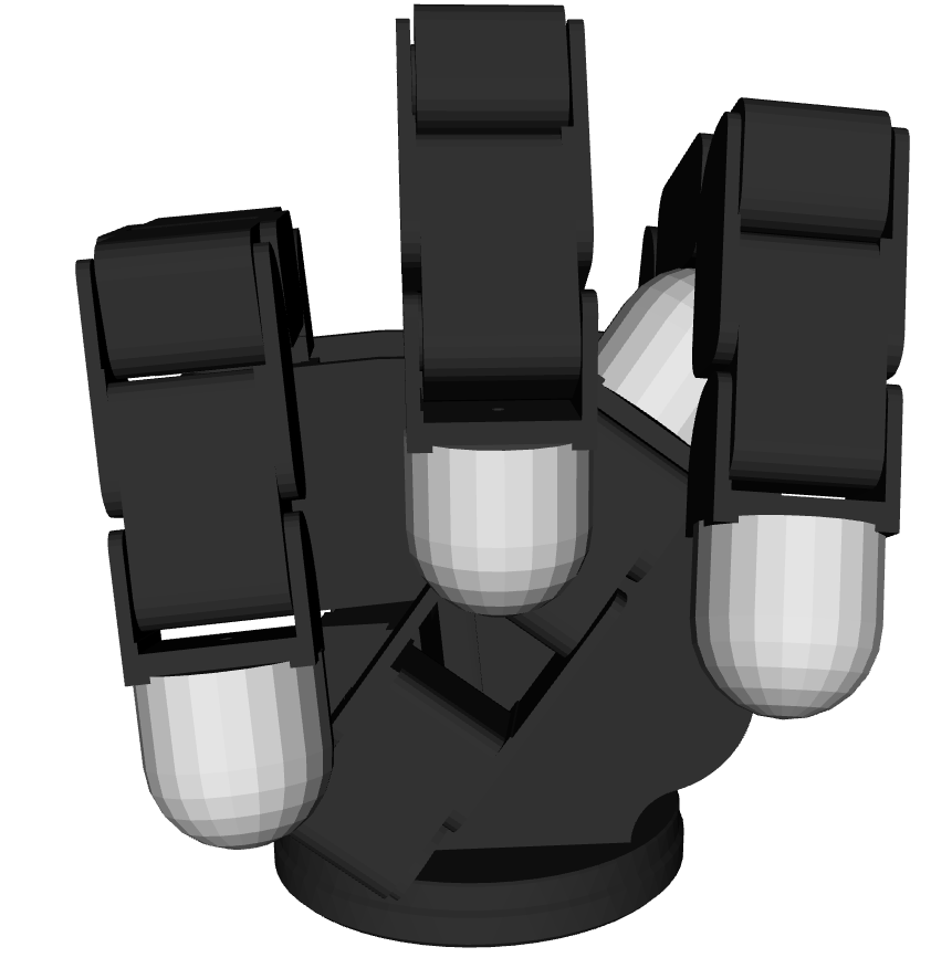
We use a 16-degrees-of-freedom (DoFs) Allegro hand model (Wonik Robotics Co., Ltd., see Fig. 3) to explain our approach in this work. The entire hand model (model mesh representation as URDF) consists of 22 geometric bodies, 5 for each finger and 2 for the palm. For simplification, we categorize these geometric bodies into 5 groups (4 fingers and 1 palm); and we consider the distances between two groups rather than the distances between geometric bodies in the following. The hand reference frame is defined at the base. Fig. 3(a) shows the X-axis by the red line and the Y-axis by the green line.

(a) Initial configuration

(b) A fist-shaped configuration

Figure 3: The Allegro robotic hand model. The hand consists of four fingers and a palm. Each finger has four joints (DoFs).

III-A2 Object model

Given the geometric models of the object, we represent the object by a set of points in space, denoted as $\bm{X}^{o}=\{\bm{x}_{i}^{o}\}_{i=1}^{N}\in\mathbb{R}^{N\times 3}$, represented in the hand frame. In practice, the point cloud of the object can be obtained using tactile or visual information.

III-B C-space representation

We describe the configuration of the $n$-DoFs robotic hand pose by its joint position vector $\bm{q}\in\mathbb{R}^{n}$. The corresponding Cartesian position of fingertips can be obtained by forward kinematics $f(\bm{q})$. If the robotic hand is composed of $m$ geometric bodies, the set of distances between any two detached geometric bodies is given by:

$$\bm{d}_{1}(\bm{q})=\{h\left(f_{i}(\bm{q}),f_{j}(\bm{q})\right)\}_{i,j=1}^{i,j=m},i\neq j,$$ (1)

where $h(\cdot,\cdot)$ outputs the shortest Euclidean distance between these two geometric bodies and $f_{i}(\bm{q})$ returns the pose of the $i$-th geometric body.

The set of distances from a point in space $\bm{x}^{o}_{i}\in\mathbb{R}^{3}$ to the geometric bodies of the robotic hand is calculated as follows:

$$\bm{d}_{2}(\bm{q},\bm{x}^{o}_{i})=\{h\left(f_{i}(\bm{q}),\bm{x}^{o}_{i}\right)\}_{i=1}^{m}.$$ (2)

Then, the minimum distance for a potential collision (either self-collision or hand-object collision) can be found through:

$$d^{\text{min}}(\bm{q},\bm{X}^{o})=\min\left(\bm{d}_{1}(\bm{q}),\left\{\bm{d}_{2}(\bm{q},\bm{x}_{i}^{o})\right\}_{i=1}^{N}\right).$$ (3)

Finally, the C-space $\mathcal{C}\in\mathbb{R}^{n}$ could be described as:

$$\mathcal{C}^{o}=\{\bm{q}\in\mathbb{R}^{n}:d^{\text{min}}<0\}$$ (4a)

$$\mathcal{C}^{b}=\{\bm{q}\in\mathbb{R}^{n}:d^{\text{min}}=0\}$$ (4b)

$$\mathcal{C}^{f}=\{\bm{q}\in\mathbb{R}^{n}:d^{\text{min}}>0\},$$ (4c)

where $\mathcal{C}^{o}$ denotes the collision region, $\mathcal{C}^{b}$ represents the collision boundary, and $\mathcal{C}^{f}$ signifies the collision-free region.

We distinguish between two types of collision: self-collision (between fingers or between a finger and the palm), and hand-object collision (between a finger or the palm, and the manipulated object). We construct distance functions for each type of collision (see Sec. III-C and Sec. III-D).

III-C Self-collision model

We train a feed-forward neural network (NN) to approximate the distance function ($\bm{d}_{1}(\bm{q})$ in Eq. (1)). Apart from estimating the distance, it is also necessary to determine whether the robot is in a collision, given its joint configuration. For this purpose, we train the NN model to output both (1) an estimation of the distance to the obstacle, and (2) a decision boundary for asserting whether the robot is in a collision.

III-C1 Dataset

to generate the training dataset, we randomly and uniformly sample the hand’s joint poses within the joint limits for every joint. Using forward kinematics, we compute the minimum Euclidean distance between two geometrical groups, according to Eq. (1). We consider the negative distance (i.e., penetration depth) a measure of collision. The sampled training dataset is pre-processed to ensure balance (see Appendix B for pre-processing of training dataset).

III-C2 NN training

we train a multi-layer feed-forward NN to estimate the mapping $\bm{q}\rightarrow\bm{d}_{1}$ with ReLU activation function and a standard mean-square weighted loss:

$$c_{1}=\frac{1}{n_{1}}\sum_{i=1}^{n_{1}}w_{j}(\bm{d}_{1,i}^{\text{nor}}-\bm{d}_{1,i}^{\text{pred}})^{2},$$ (5)

The weights $\bm{w}=\{w_{j}\}_{j=1}^{3}$ are set to different values based on $\bm{d}_{1,i}^{\text{nor}}$ and $\bm{d}_{1,i}^{\text{pred}}$ as in Table. I. For example, $\bm{w}=[0.1,6,4]$. In this way, the false positives (FP) and false negatives (FN) are penalized, which could improve the accuracy in the binary classification for collision detection and the regression accuracy for distances close to zero. Since we prioritize safety, accuracy is not a major concern when the prediction distance and ground truth both exceed 0.5, as this indicates a safe distance from collisions. In these instances, we can set $w$ to 0.1 in the cost function to minimize the impact of prediction errors. A grid search is conducted to determine the optimal structure of the NN model (see Appendix C for evaluation of trained NN model).

TABLE I: Weights for the cost function of self-collision model.

	$\bm{d}_{1,i}^{\text{pred}}\leq 0$	$0<d_{1,i}^{\text{pred}}\leq 0.5$	$d_{1,i}^{\text{pred}}>0.5$
$\bm{d}_{1,i}^{\text{nor}}\leq 0$	$w_{1}$	$w_{2}$	$w_{2}$
$0<\bm{d}_{1,i}^{\text{nor}}\leq 0.5$	$w_{3}$	1	1
$\bm{d}_{1,i}^{\text{nor}}>0.5$	$w_{3}$	1	$w_{1}$

III-D Hand-object collision model

To estimate collisions between the hand and an external object, we train a model of the distance function Eq. (2). We hence train a total of 3 NNs to determine the distance of the point object to the palm, thumb, and index finger. Notice that the index, middle, and ring fingers use the same NN as these fingers share identical geometric and kinematic models.

III-D1 Dataset

we generate a uniform distribution of arbitrary points $\bm{x}^{o}$ from scaled cuboid hulls (1.1, 2, and 5 times) of hand geometries. We randomly select joint positions, update the pose of each geometric body using forward kinematics, and randomly select $\bm{x}^{o}$ from within the resulting cuboid hulls. The distance between each geometric body and a point in space is calculated using the Trimesh library [7].

Three datasets are generated for the palm, the index finger, and the thumb finger, which are denoted as $\bm{D}_{k}=\{(\bm{q}_{i},\bm{x}^{o}_{i}),\bm{d}_{2,i}^{r}\}_{i=1}^{n_{k}},k=2,3,4$, respectively. The datasets are processed similarly to Sec. III-C2 for training the NN model.

III-D2 NN training

Three fully-connected NNs are trained to estimate the mappings $(\bm{q},\bm{x}^{o})\rightarrow\bm{d}_{2}$ for distance estimation. We follow the same training procedure as described in Section III-C2 (see Appendix D for model evaluation).

Finally, a NN-based estimation of Eq. (3) is achieved as $\hat{d}^{\text{min}}(\bm{q},\bm{X}^{o})$, by combining the self-collision model and the hand-object collision model. As the fully-connected NNs of 4 layers are adopted with ReLU, the gradient of the distance with respect to a joint could be derived in realtime.

IV Sampling-based Motion Planning

We first present a dynamical system (DS) based real-time motion planning approach with collision avoidance in C-space (Sec. IV-A). Then, to address the challenge of potential local minima, we integrate a sampling-based solution into the DS and call it DS-guided RRT* (Sec. IV-B). Finally, a dynamic PRM* is proposed by leveraging the gradients of the distances from the NNs (Sec. IV-C).

IV-A DS-based obstacle avoidance

(a)

(b)

Figure 4: An example of DS-based motion planning. (a): Side view of the start (non-transparent figure) and the goal (transparent, finger most bend) configurations of the hand. The middle finger must bend to avoid a spherical obstacle (the red dot). (b): Isolines and DS streamlines in C space, visualized in a 2D space ($q_{2}$, $q_{3}$). The black curve is the obstacle boundary. The blue and red points show the start and end configurations of the joints. The color bar refers to the normalized spatial distance between the obstacle and the finger at the corresponding configuration. DS streamlines illustrate the velocity field.

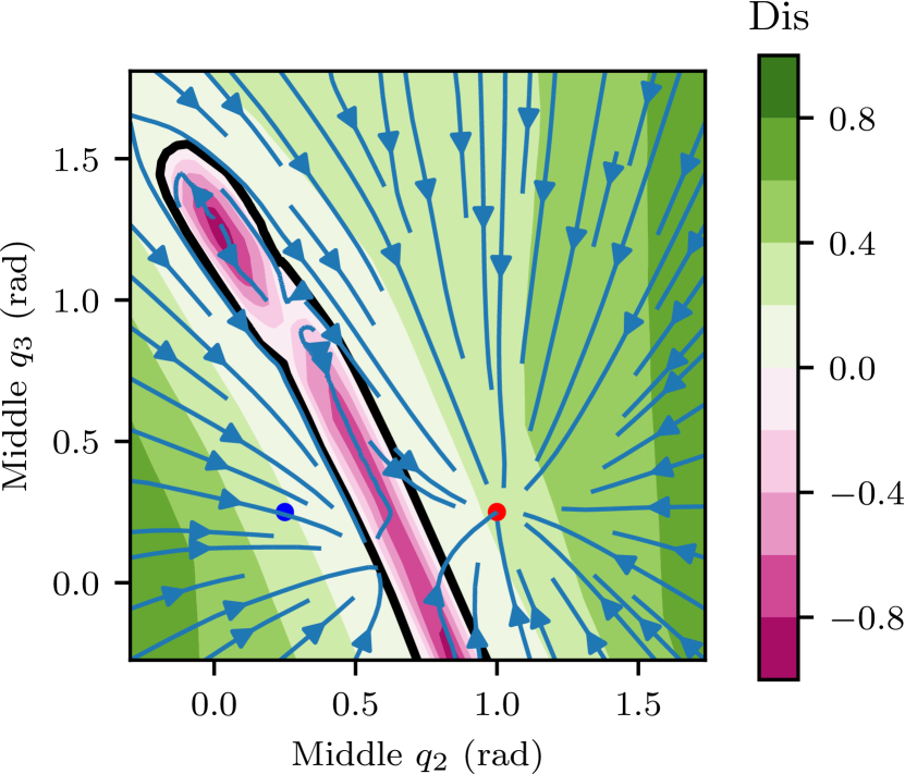
Inspired by [Mohammad2012DS_modulation], we build a close-loop control system composed of a linear vector field to the desired joint configuration $\bm{q}_{g}$, given by a first-order differential equation, as follows:

$$\dot{\bm{q}}=\bm{f}(\bm{q})=\bm{A}(\bm{q}-\bm{q}_{g}).$$ (6)

$\bm{A}$ is negative-definite. The dynamics has a single fixed point, hence the robot motion is guaranteed to reach and stop at $\bm{q}_{g}$. The vector field can be deflected by the gradient of the distance to obstacles to avoid them, with larger deflection when closer to the boundary with the collided space. To use [Mohammad2012DS_modulation] formalism, we construct a scaled distance function to the collided space boundary using our learned distance function:

$$\Gamma(\bm{q},\bm{x})=\alpha_{1}(d^{\text{min}}-d_{\text{safe}})+1.$$ (7)

We compute the analytic gradient of $\Gamma$ with respect to $\bm{q}$, as $\frac{\partial\Gamma}{\bm{q}}=\alpha_{1}\frac{\partial d}{\partial\bm{q}}$, by first-order derivation of the NNs decision function. $d_{\text{safe}}$ is a safety margin of the distance. $\alpha_{1}$ is a positive scaling factor. To deflect the dynamics in the vicinity of the collided space boundary, we use the direction formed by the gradient of our distance function. We project onto a basis composed of the tangents and normal to the boundary of the collided space, which is given into matrix E, see [Mohammad2012DS_modulation]:

$$\dot{\bm{q}} =\bm{E}\bm{D}\bm{E}^{-1}f(\bm{q}),$$ (8)

$$\text{with \quad}\bm{E} =\left[\frac{\partial\Gamma}{\partial\bm{q}},\;\;\bm{e}^{2},\cdots,\;\;\bm{e}^{n}\right],$$

$$\bm{D} =\left[\begin{matrix}\lambda^{1}&&\bm{0}\\ &\ddots&\\ \bm{0}&&\lambda^{n}\end{matrix}\right].$$

The columns of $\bm{E}$ are composed of n sets of vectors forming a basis of the joint space, with the first column aligned with the normal to the boundary. $\bm{D}$ is a diagonal matrix. The eigenvalues are designed in such a way that the flow vanishes along the normal once it reaches the boundary, hence preventing the robot from penetrating the obstacle:

$$\left\{\begin{aligned} \lambda^{1}&=1-\frac{1}{|\Gamma|^{\frac{1}{\rho}}}\\ \lambda^{i}&=1+\frac{1}{|\Gamma|^{\frac{1}{\rho}}}\quad 2\leq i\leq n\end{aligned}\right.,$$ (9)

where $\rho>0$ is a reactivity parameter that can be tuned to modulate the sharpness of the deflection around the boundary.

The above approach is guaranteed to have no stable point, except at the desired configuration where the obstacle is convex in C space (See the proof in [Mohammad2012DS_modulation]). When computing deflection in a high-dimensional C-space, it arises often that the boundary displays strong concavities. Hence, it occurs often that the dynamics stops. This is illustrated in Fig. 4(a). Even if the obstacle is convex (here spherical) in Cartesian space, the obstacle creates a concave shape in C-space, as shown in Fig. 4(b). Motions that start from the left-bottom region of the obstacle in Fig. 4(b) will become trapped in a local minimum instead of converging towards the attractor.

Input: $\bm{q}_{a}$, $\bm{X}_{obs}$, $\bm{q}_{g}$,

Parameters : $0<\alpha_{2}<1$, $i_{\text{max}}>0$

1 Initialize $\mathcal{T}$ by $\bm{q}_{a}$,
while not reaching the goal and $i<i_{\text{max}}$ do

2       update $\bm{q}_{a}$, $\bm{X}_{obs}$, $\bm{q}_{g}$

3       $\bm{d}_{n}(\mathcal{T}_{n}):=\hat{d}^{\text{min}}(\mathcal{T}_{n},\bm{X}^{o})$

4       $\mathcal{T}_{n}^{f}:=\{\bm{q}\in\mathcal{T}_{n}:\bm{d}_{n}(\bm{q})>d_{\text{safe}}\}$

5       $\mathcal{T}_{n}^{o}:=\{\bm{q}\in\mathcal{T}_{n}:\bm{d}_{n}(\bm{q})\leq d_{\text{safe}}\}$

6      

7      $\bm{d}_{e}(\mathcal{T}_{e}):=\hat{d}^{\text{min}}(\mathcal{T}_{e},\bm{X}^{o})$

8       remove edges in $\mathcal{T}_{e}$ where $\bm{d}_{e}(\mathcal{T}_{e})\leq d_{\text{safe}}$

9       a rewire list $\bm{Q}_{\text{rewire}}$ := $\{\bm{q}\in\mathcal{T}_{n}:$ the node $\bm{q}$ has different collision state with the last iteration}

10      

11      if no feasible path then

12             $\bm{Q}_{\text{rand}}\leftarrow Sample(\mathcal{C})$

13             $\bm{Q}_{\text{nearest}}\leftarrow Nearest(\bm{Q}_{\text{rand}},\mathcal{T}_{n}^{f})$

14             update $\delta q$ by Eq. (10) for each $\bm{q}_{\text{nearest}}$

15             $\bm{Q}_{\text{new}}:=\bm{Q}_{\text{nearest}}+\delta\bm{q}\bm{n}_{q}$

16             get nearby nodes and calculate costs from $\bm{q}_{0}$ to $\bm{q}_{\text{new}}\in\bm{Q}_{\text{new}}$ by $\bm{q}_{\text{near}}$

17             connect all possible $\bm{q}_{\text{new}}$ with the best collision-free parents

18            

19       rewire the nodes nearby $\bm{Q}_{\text{rewire}}$

20       Run Algorithm 2 with 10% probability

21       Robot moves by Algorithm 3

22      

23      $i:=i+1$

24 end while

Algorithm 1 DS-guided RRT*

IV-B DS-guided RRT*

Algorithm. 1 illustrates the steps to apply our proposed DS-guided RRT*. $\mathcal{T}$ refers to the tree, where $\mathcal{T}_{n}$ are nodes in $\mathcal{C}$ and $\mathcal{T}_{e}$ are edges. At each iteration, the positions of the obstacle, current robot joints $\bm{q}_{a}$ and the goal $\bm{q}_{g}$ are updated (Line 1). Then the minimum distances of all nodes are estimated by NNs, with an update of the collision-free nodes $\mathcal{T}_{n}^{f}$ and collided nodes $\mathcal{T}_{n}^{o}$ (Line 1-1). For each edge in $\mathcal{T}_{e}$, uniform samples are performed and inputted to NNs for collision check of edges (Line 1), where edges under collision are removed from the tree (Line 1). To handle an environment with moving obstacles, a rewire list is established and populated with nodes whose collision states have changed from the previous iteration. These nodes will be utilized for RRT rewiring. In case of an infeasible path, tree expansion is necessary to search the space. A fixed number of nodes are randomly selected from $\mathcal{C}$ (Line 1) and their nearest nodes are found in $\mathcal{T}n^{f}$. At each node $\bm{q}=\bm{q}_{\text{nearest}}$ in $\bm{Q}_{\text{nearest}}$, a first-order approximation of the distance function is used. To improve the efficiency of RRT exploration, the stepsize is adjusted dynamically with the following constraint:

$$\alpha_{2}\bm{d}(\bm{q}_{\text{nearest}})+\delta q\left.\bm{n}_{q}^{T}\frac{\partial\bm{d}}{\bm{q}}\right|_{\bm{q}=\bm{q}_{\text{nearest}}}>d_{\text{safe}},$$ (10)

where the vector $\bm{n}_{q}$ represents the normalization of $\bm{q}_{\text{rand}}-\bm{q}_{\text{nearest}}$. The update step is bounded $\delta q_{l}\leq\delta q\leq\delta q_{u}$ to avoid extreme values. $\alpha_{2}\in[0,1]$ is a constant coefficient. We use $\alpha_{2}=0.5$ in this work. When $\bm{n}_{q}$ and the gradient $\left.\frac{\partial\bm{d}}{\bm{q}}\right|{\bm{q}=\bm{q}_{\text{nearest}}}$ form an acute angle, $\delta q$ is set to the maximum value $\delta q_{u}$ for greedy exploration. Otherwise, $\delta q$ is reduced following Eq. (10) to allow for more reliable exploration.

The variable stepsize for each $\bm{q}=\bm{q}_{\text{nearest}}$ allows us to create a list of pending nodes $\bm{Q}_{\text{new}}$ (Line 1). Similar to the RRT* algorithm [karaman2011sampling], we calculate the cost from the start point to each node $\bm{q}_{\text{new}}\in\bm{Q}_{\text{new}}$ by evaluating its nearby nodes. The nearby node with the lowest cost is selected as the parent of $\bm{q}_{\text{new}}$. The tree is then updated with the new nodes and edges, and an RRT*-like rewiring process is applied to the list $\bm{Q}_{\text{rewire}}$ for guaranteed optimality (Line 1).

In Algorithm 2, we adopt a DS-based solution check that differs from traditional straight-line checks. The list of nodes to be checked is initialized by merging the last feasible nodes $\bm{Q}_{\text{DS}}$ and new nodes $\bm{Q}_{\text{new}}$ (Line 2). Over $K$ iterations of integrating differential Eq. (8) (Line 2), $\bm{Q}_{0}$ progresses to $\bm{Q}_{K}$ along the modulated DS. If any nodes approach the goal $\bm{q}_{g}$, the original nodes are stored in $\bm{Q}_{\text{DS}}$.

Finally, the algorithm attempts to find a feasible path. If the list $\bm{Q}_{\text{DS}}$ is not empty, indicating that the DS has guided some nodes towards the goal, then a feasible path exists. The node $\bm{q}_{k}$ with the lowest cost is selected as an intermediate point towards the goal. If $\bm{q}_{k}$ is the root of the tree $\mathcal{T}$, the robot will move along the DS (Line 3), otherwise, it will follow the tree (Line 3). If $\bm{Q}_{\text{DS}}=\varnothing$, the algorithm determines that no feasible path exists and the robot remains stationary (Line 3).

Input: $\bm{Q}_{\text{new}}$, $\bm{d}$, $\frac{\partial\bm{d}}{\bm{q}}$, $\bm{q}_{g}$,

Parameters : $0<{\delta t}\leq 0.01$, $\epsilon=1e^{-4}$, $K=50$,

1 $\bm{Q}_{0}:=\{\bm{q}\in\bm{Q}_{\text{DS}}\text{ or }\bm{q}\in\bm{Q}_{\text{new}}\}$
for $i\leftarrow 0$ to $K$ do

2       update $\dot{\bm{Q}}_{i}$ by Eq. (8) for every $\bm{q}\in\bm{Q}_{i}$

3       $\bm{Q}_{i+1}:=\bm{Q}_{i}+\dot{\bm{Q}}_{i}{\delta t}$

4       $\bm{Q}_{\text{DS}}:=\{\bm{q}\in\bm{Q}_{0}:\|\bm{q}_{i+1}-\bm{q}_{g}\|<\epsilon\}$

5       if $\bm{Q}_{\textsc{DS}}\neq\varnothing$ then

6             break

7      

8 end for

9

return $\bm{Q}_{\textsc{DS}}$

Algorithm 2 Solution check by the integral of DS

Input: $\mathcal{T}$, $\bm{Q}_{\text{DS}}$

1

2if $\bm{Q}_{\textsc{DS}}\neq\varnothing$ then

3       find $\bm{q}_{k}\text{ with minimum cost to the root by }f_{c}(\bm{q})=\text{cost}(\bm{q}_{0},\bm{q}),\bm{q}\in\bm{Q}_{\text{DS}}$

4       if $f_{c}(\bm{q}_{k})==0$ then

5            move along DS modulation by Eq. (8).

6       else

7             retrieve the path from $\bm{q}_{0}$ to $\bm{q}_{k}$ by finding the parent inversely

8             move toward $\bm{q}_{0}$

9             if $\bm{q}_{a}$ close to $\bm{q}_{0}$ then

10                   $\bm{q}_{0}:=\bm{q}_{1}$

11                   rewire to set $\bm{q}_{0}$ as the root

12            

13       end if

14      feasible path exists

15 else

16       stay at $\bm{q}_{0}$; no feasible path

17      

18 end if

19

Algorithm 3 Find a feasible path

IV-C Dynamic PRM*

Taking advantage of the gradients in C-space, we can update a portion of the nodes in the PRM* online, bringing them closer to the collision boundary. This results in the discovery of a shorter and more feasible path.

Considering one node $\bm{q}$ in PRM*, the minimum distance to the obstacle boundary and its gradient with respect to $\bm{q}$ are calculated from NNs. Given this, the node is adjusted to the following one:

$$\bm{q}\leftarrow\bm{q}-\beta\frac{\hat{d}^{\text{min}}(\bm{q})-\beta_{2}d_{\text{safe}}-\frac{\partial\hat{d}^{\text{min}}}{\partial\bm{x}^{o}}(\delta\bm{x}^{o})}{\frac{\partial\hat{d}^{\text{min}}}{\partial\bm{q}}},$$ (11)

where let $0<\beta_{1}<1$ is the adjustment step coefficient factor. If the obstacle is static or the minimum distance is from the self-collision model, then $\frac{\partial\hat{d}^{\text{min}}}{\partial\bm{x}^{o}}=0$. This allows the node to update and move in the direction opposite to the gradient until $\hat{d}^{\text{min}}(\bm{q})=\beta_{2}d_{\text{safe}}$. The safety factor $\beta_{2}>1$ ensures a secure margin. Notably, the distance queries and gradient computations are efficiently performed in parallel by NNs, enabling real-time node adjustments through parallel matrix computations of Eq. (11). As the nodes is changing under the scenario of moving obstacles, the roadmap is also updated online by a GPU-accelerated k-NN.

V Simulations and experiments

We validate our proposed algorithms both in simulation and on a real robotic hand. We first systematically evaluate the performance of our proposed collision detector based on our C-space representation (Sec. V-A). Then, we compare our sampling-based motion planning approach to state-of-the-art approaches (Sec. V-B). Finally, we demonstrate the effectiveness of our approaches on a real robotic hand for online collision avoidance (Sec. V-C).

V-A Comparisons of collision detection

We use the FCL as a baseline for collision detection. The computational performance is investigated and the results are shown in Table. II. Considering the Allegro hand with a random joint configuration in 16D and a random point in the workspace, both self-collision and hand-point collision are counted in the time cost.

The FCL time cost increases almost linearly along the batch size, while the NN-based method shows a significantly faster detection. One reason is that FCL needs to compute the forward kinematics for updating poses for all geometric bodies, and then calculate the minimum distance, which is computationally intensive. NN-based collision detection can achieve a query interface of over 100 Hz for 10,000 samples.

TABLE II: Comparison of computational time cost (in milliseconds) for different methods of collision detection.

Sample size	FCL	NN by CPU	NN by GPU
1	11.0	1.3	5.4
10	110.2	1.7	5.4
100	238.4	2.8	5.8
1,000	1167.3	8.3	5.8
10,000	11448.5	31.4	8.5
100,000	122005.7	458.5	45.7
1,000,000	1189485.1	4531.8	412.4

V-B Simulations of sampling-based methods

We compare our motion planning approaches with the following commonly used approaches:

1. RRT* [karaman2011sampling] combines the original RRT method with rewiring to generate optimal paths.

2. P-RRT* [qureshi2016potential] uses a potential field approach to guide sampling in RRT*.

3. RRT* using a variable stepsize as in Eq. (10).

4. PRM* [karaman2011sampling].

Metrics include success rate, computation time, and the length of a feasible path. Both static and dynamic environments are tested in 2D and 16D spaces. For RRT-based methods, maximum nodes $i_{\text{max}}=1000$. In PRM-based methods, the number of samples is set as 200. All methods are able to use the learned distance functions for collision detection, while our methods exploit the gradients of the distance functions.

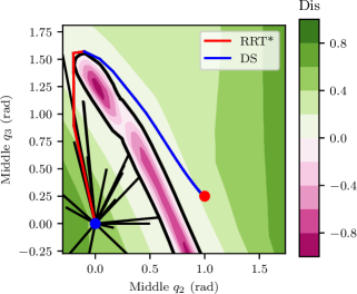
First, considering a 2D and static scenario as Fig. 4(a), a feasible path from DS-guided RRT* is shown in Fig. 5, where the path consists of several RRT-based straight lines (in red) and a DS-guided curve (in blue) to the goal. At the junction point, if a solution check by a straight line to the goal is tried, the collision checker will return the collision state, and thus more RRT samples are required. Comparisons with metrics are recorded in Tab. III with 100 trials for each. All the RRT-based methods have a 100% success rate. The DS-guided RRT* does not return an optimal path and has a longer path length than others. However, it shows a faster computation time than other RRT methods thanks to the variable stepsize and the solution check by DS. Because of the narrow passage, PRM* shows a lower success rate, which is slightly improved by the dynamic PRM*. Taking advantage of parallel computing, PRM-based methods are much faster than RTT-based ones, where the computation time includes updating nodes, building the roadmap, and finding a feasible path by PRM*.

Figure 5: An example of a DS-guided RRT* search in C-space projected 2D space of ($q_{2}$, $q_{3}$). The black line segments represent the sampled paths, while the feasible path from the start (blue dot) to the goal (red dot) is a combination of the straight lines generated by RRT* and the blue curve from DS.

(a)

(b)

(c)

(d)

(e)

Figure 6: An illustration of controlling a 16-DoF hand to move from an open configuration in (a) to a fist-shaped configuration in (e), while avoiding collisions with four spatial obstacles represented by red dots, as well as collisions between the fingers.

A 16D scenario is set up as Fig. 6. Considering a task to clench the fist shape from fully open to Fig. 6(e), there are four spherical obstacles on the way of each finger. Both self-collision and hand-object collision should be taken into account, with narrow passages for motions. Tab. IV illustrates the simulation results. Traditional RRT-based methods suffer from high dimension problems and have a very poor success rate, while the DS-guided RRT* is able to keep the 100% success rate but still returns a longer path. On the other hand, dynamic PRM* offers a shorter path than PRM*. The computation time is not affected by the high dimension. Compared to the work by [yeh2012uobprm], where the gradients are not available and nodes are sampled by intersections between random segments and C- obstacles, the dynamic PRM* takes about 0.15 s for computation, rather than a few seconds.

For dynamic environments, the DS-guided RRT* and dynamic PRM* are able to update the collision states for all nodes and query a path within 30 ms. Note that both methods are suitable for multi-query tasks, while other methods need to compute a path by full initialization, and the time cost is equal to the computation time in Tab. III and Tab. IV.

TABLE III: Comparison of computational performance of different search algorithms in a 2D static case illustrated by Fig. 4(a).

	Success rate	Computation time (s)	Path length (rad)
RRT*	1	1.56 (1.16)	3.73 (0.17)
P-RRT* [qureshi2016potential]	1	1.88 (0.87)	3.70 (0.14)
RRT* with variable step	1	1.06 (0.57)	3.82 (0.24)
DS-guided RRT*	1	0.99 (0.52)	4.06 (0.74)
PRM* [karaman2011sampling]	0.55	0.10 (0.03)	3.66 (0.06)
Dynamic PRM*	0.7	0.17 (0.03)	3.65 (0.05)

TABLE IV: Comparison of computational performance of different search algorithms in a 16D static case.

	Success rate	Computation time (s)	Path length (rad)
RRT*, P-RRT*	0.02	-	-
RRT* with variable step	0.17	47.81 (12.95)	6.33 (0.59)
DS-guided RRT*	1	1.61 (1.45)	13.28 (3.5)
PRM* [karaman2011sampling]	0.8	0.15 (0.01)	8.64 (1.77)
Dynamic PRM*	0.8	0.15 (0.00)	8.47 (1.56)

V-C Evaluation on a real robotic hand

We evaluated our proposed approaches in two experimental tasks with a real Allegro robotic (left) hand. We used a glue stick (cylindrical shaped, radius 8mm, length 147mm). The robotic hand was stably mounted upright on a table surface through a stand, such that the fingertips point upwards when the hand is fully opened (see Fig. 2). $\text{OptiTrack}^{\text{\texttrademark}}$ motion capture system was used for spatial localization. For this purpose, four markers were attached to the base of the hand to localize the hand reference frame; and three markers were attached to the object surface to track the object pose in real-time. The object was represented by 100 spheres along its axis with a radius of 8mm. Spatial positions were represented in the hand frame.

V-C1 Reactive collision avoidance

The first experimental scenario aims at evaluating the performance of our proposed algorithm for real-time collision avoidance in 16D. Fig. 8(a) illustrates the experimental setup and the initial state of the robotic hand. The experimental object was attached to the end of a long stick. The spatial position and orientation of the object were detected by the motion capture system in real-time. A human experimenter held the stick to move the object toward the hand and tried to collide with the index finger (Fig. 8(a)). A collision is about to happen and needs to be avoided, if (1) the predicted distance between the experimental object and the hand, or (2) the distance between any pair of two fingers, reduces below the safety margin ($5$mm in this experiment). In this case, the hand performed an adjustment motion along the direction of $\frac{\partial\hat{d}^{\text{min}}}{\partial\bm{q}}$, which indicates the fastest direction to increase the distance $\hat{d}^{\text{min}}$ and to avoid a collision (see Fig. 8(b),(c)).

In a second experimental trial (Fig. 8(d),(e),(f)), the experimenter held the stick and tried to collide with all three fingers from the back (Fig. 8(d)), and then adjusted pose to approach the thumb (Fig. 8(e)). Notice that in Fig. 8(e) and (f), both the middle and the ring fingers moved away from the object, even though the object did not approach them. This is because the index finger moved to avoid a potential collision with the object, causing the distance between adjacent fingers to reduce. Hence, all fingers moved to avoid self-collisions, i.e., collisions between adjacent fingers, guided by the gradient from our self-collision model.

(a)

(b)

(c)

(d)

(e)

(f)

Figure 8: Assessing the reactive collision avoidance approach on Allegro hand. Each row represents a trial. A glue stick (experimental object) approaches the hand. The hand is controlled to avoid both collisions with the object and inter-finger collisions. In scenarios (a) to (c), the object moves between two fingers, while in (d) to (f), it approaches the hand from the back towards the front and side of the fingers.

V-C2 Collision-free motion planning for changing grasp pose

In this scenario, the goal is to change the grasp pose from a thumb-index pinch grasp (see Fig. 10(a)) to a four-finger pinch grasp (see Fig. 10(d)) by changing the placement of fingers. We assume that the grasp remains stable during all intermediate states, allowing the object to be held without being dropped. This task is challenging because the ring finger needs to move from above to below the object within a very limited space inside the hand (Fig. 10).

The thumb and the index finger were controlled to remain in the same joint configuration. We only generated collision-free trajectories for both the middle and the ring fingers, leading to an 8D online motion planning problem. Two different solutions were generated to achieve the task goal. In one solution (Fig. 10(a)-10(d)), the ring finger moves to the right side of the held glue stick to avoid potential collisions. An alternative solution is illustrated in the first row of Fig. 2, where the ring finger moves left and then bends to avoid a collision; the middle finger also moves left to make space for the ring finger. Finally, both fingers arrived at the desired configuration.

(a)

(b)

(c)

(d)

Figure 10: An example of a collision-free finger replacement: the ring finger moves to the right side of the grasped object to avoid collision and arrive at the desired configuration to grasp.

VI Discussion and conclusion

In this study, we addressed the challenges of real-time collision-free path planning for multi-fingered robotic hands during in-hand manipulation, with a particular focus on changing grasping poses. To ensure a collision-free path in a cluttered and dynamic environment, we proposed an NN-based approach for accurately representing the C-space and detecting collisions in real-time. Our method utilizes the estimated distances and their gradient in C-space to guide a sampling-based motion-planning, RTT*, via DS. This combination of DS and RRT* led to improved success rates for high-dimension problems. Additionally, we have developed a dynamic PRM* approach that leverages parallel computation to enhance performance. Experimental results demonstrate that our approaches offer effective solutions for real-time collision-free path planning for a multi-fingered robotic hand. It is noteworthy to mention that the application domains of our model extend beyond collision avoidance, as it offers a precise depiction of the object’s boundary and its tangent. This representation potentially enables the planning of finger trajectories for a sliding motion on the object’s surface, or impedance control during manipulation given a specific penetration distance. Our future work involves generalizing our current approach to a wider range of robotic systems and objects, and exploring its potential for various tasks, such as dexterous in-hand manipulation that requires the coordinated motion of all fingers.

Our paper presented two robotics motion planning algorithms, DS-guided RRT* and dynamic PRM*. While DS-guided RRT* can be implemented in real-time and improve the success rate in high dimensions, it may not result in the shortest possible path. On the other hand, Dynamic PRM* improves the performance of PRM* but may fail at finding a path in narrow passages that arise frequently in highly cluttered environments, a common limitation of PRM*. In a robotic implementation, failure cases may arise due to inaccuracies in localizing the object pose and tracking the robot’s trajectory. These limitations highlight the need for further research in motion planning to overcome the current challenges and produce more optimal and efficient solutions.

Appendix A Technical Notes

In Sec. V-A, for batch sizes greater than or equal to 100, FCL is executed by 20 processes. The NN-based collision detector was run on an Intel Core i7-12700HQ CPU and RTX3070ti GPU. The Allegro robotic hand was connected to an Ubuntu 20.04 laptop and controlled by a joint position PID controller in ROS Noetic at 200 Hz.

Appendix B Pre-processing of training dataset for self-collision NN model

A critical point when generating such a dataset is balancing the collision and collision-free classes. We balance the dataset by ensuring that only half of the samples are collision-free. It takes 3 hours to generate 2 million samples with an Intel Core i7-12700HQ CPU (20 processes). The dataset is denoted as joint-distance pairs $\bm{D}_{1}=\{\bm{q}_{i},\bm{d}_{1,i}^{r}\}_{i=1}^{n_{1}}$ with $n_{1}$ samples and $\bm{d}_{1,i}^{r}\in\mathbb{R}^{10}$.

To improve the accuracy and convergence speed of the NN, the dataset is scaled by min-max normalization for positive and negative distances separately, which is written as:

$$\bm{d}_{1,i}^{\text{nor}}=\left\{\begin{matrix}&{\bm{d}_{1,i}^{r}}/{\bm{d}_{1}^{\text{up}}},\quad\bm{d}_{1,i}^{r}\geq 0\\ &{\bm{d}_{1,i}^{r}}/{\bm{d}_{1}^{\text{low}}},\quad\bm{d}_{1,i}^{r}<0\end{matrix}\right..$$ (12)

Rather than using the minimum and maximum distances for normalization, we established the upper bound $\bm{d}_{1}^{\text{up}}$ and lower bound $\bm{d}_{1}^{\text{low}}$ empirically, based on the distributions of each column in the dataset.

Appendix C Evaluation of self-collision NN model

Figure 11: Evaluating the Accuracy of Neural Networks with Different Architectures through Cross-Validation. The bar graph displays the mean accuracy of 20 trials, each trained for 10,000 epochs, of various neural network structures. The height of each bar indicates the mean accuracy, while the error bars represent the standard deviation. The x-axis labels denote the number of neurons used in each neural network structure.

Figure 12: Heatmap for a grid search on the false positive rate (FP). The goal is to determine the optimal values of the weights $w_{2}$ and $w_{3}$ in the cost function given by Eq. (5). The $(w_{2},w_{3})$ pair with the lowest FP is highlighted in white.

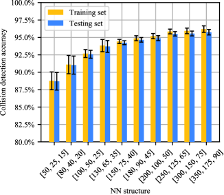
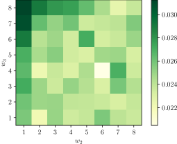
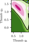
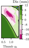
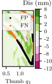
To evaluate our model’s performance, we divide our dataset into two parts: $50\%$ for training and $50\%$ for testing, each containing 1 million samples. The training process involves 20,000 iterations to optimize the network’s parameters. Fig. 11 illustrates the cross-validation results with increasing layer widths. NNs with 2 layers and 4 layers are also tested. The accuracies are not significantly improved after the layer widths of $[350,175,90]$. To determine the weights in Eq. (5), we performed a grid search for $(w_{1},w_{2})$ (see Fig. 12).

TABLE V: Evaluation of the self-collision model presented in terms of False Positives (FP) and False Negatives (FN), where the positive class is the collision-free state, and the negative one indicates the presence of self-collision.

Collision detection accuracy	FP	FN	Regression error (mm)	FP with 3 mm margin	FP with 5 mm margin
96.5%	2.61%	4.12%	0.63 (0.94)	0.22%	0.029%

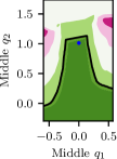
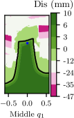
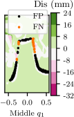
Then we run the validation on another 1 million samples. To get back the real distances, we invert Eq. (12). Table. V shows the collision detection accuracy. We evaluate the sensitivity of our distance function in determining the minimum safety distance to the boundary that minimizes false positives (FP), i.e., poses incorrectly classified as non-collided, across collided and free space. When the safety margin of the distance $d_{\text{safe}}$ is $0$, the ratio of FP is $2.61$%. For $d_{\text{safe}}$ equal to $3$mm or $5$mm, the FP decreases significantly. We hence set such margin for our experiments (See Fig. 14).

(a) NN prediction

(b) Ground truth

(c) Error

Figure 14: C-space visualization under the fist-shaped configuration of Fig. 3(b) with distance isolines. (a) 1st column: The C space calculated by the NN. (b) 2nd column: The C space of groundtruth. (c) 3rd column: Distance prediction error. 1st row: The 1st and 2nd joints of middle finger. 2nd row: The 1st and 3rd joints of Thumb finger. The blue point refers to the current robot joints and the black curve is the collision boundary. The predicted C space is almost the same as the ground truth. FP and FN samples occur nearby the boundary. Thus, increasing the safety margin could reduce the FP rate.

Appendix D Evaluation of hand-object collision NN model

TABLE VI: Evaluation of the hand-object collision model. The collision-free state is referred to as the positive class, while the negative class indicates the existence of a collision.

	Collision detection accuracy	FP	FN	Regression error (mm)	FP with 5 mm margin
Palm	98.0%	0.23%	2.3%	0.74 (0.63)	0
Index	96.4%	2.9%	3.7%	0.86 (0.75)	2.8 e-6
Thumb	95.4%	2.9%	5.3%	1.02 (0.97)	8.9 e-6

The evaluation results are shown in Table. VI. The accuracy of the NN for the index and thumb fingers is comparable to that of the palm model (98%), which has the highest accuracy due to its static nature that is not impacted by joint movements. For the three NNs, FP rates reduce to a marginal number when using 5 mm as the safety margin. We denote the three NNs distance functions as$\hat{\bm{d}}_{k}(\bm{q},\bm{x}^{o}),k=2,3,4$ for the distances between the point $\bm{x}^{o}$ and the palm, index, and ring finger, respectively.

References

- Andrychowicz et al. [2020] OpenAI: Marcin Andrychowicz, Bowen Baker, Maciek Chociej, Rafal Jozefowicz, Bob McGrew, Jakub Pachocki, Arthur Petron, Matthias Plappert, Glenn Powell, Alex Ray, et al. Learning dexterous in-hand manipulation. The International Journal of Robotics Research, 39(1):3–20, 2020.
- Bicchi [2000] Antonio Bicchi. Hands for dexterous manipulation and robust grasping: A difficult road toward simplicity. IEEE Transactions on robotics and automation, 16(6):652–662, 2000.
- Bohlin and Kavraki [2000] Robert Bohlin and Lydia E Kavraki. Path planning using lazy PRM. In Proc. IEEE Intl Conf. on Robotics and Automation (ICRA). Symposia proceedings (Cat. No. 00CH37065), volume 1, pages 521–528. IEEE, 2000.
- Brock [1988] David L Brock. Enhancing the dexterity of a robot hand using controlled slip. In Proc. IEEE Intl Conf. on Robotics and Automation (ICRA), pages 249–251. IEEE, 1988.
- Cherif and Gupta [1998] Moëz Cherif and Kamal K Gupta. 3D in-hand manipulation planning. In Proc. IEEE Intl Conf. on Robotics and Automation (ICRA). Innovations in Theory, Practice and Applications (Cat. No. 98CH36190), volume 1, pages 146–151. IEEE, 1998.
- El-Khoury et al. [2013] Sahar El-Khoury, Miao Li, and Aude Billard. On the generation of a variety of grasps. Robotics and Autonomous Systems, 61(12):1335–1349, 2013.
- [7] Dawson-Haggerty et al. Trimesh. https://trimsh.org/.