OMOD: An open-source tool for creating disaggregated mobility demand based on OpenStreetMap

Abstract

This paper introduces OMOD (OpenStreetMap Mobility Demand Generator), a new open-source activity-based mobility demand generation tool. OpenStreetMap Mobility Demand Generator (OMOD) uses a data-driven approach, calibrated with household travel survey data, to generate a population of agents with detailed daily activity schedules that state what activities each agent plans to conduct, where, and for how long. The temporal aspect of the output is wholly disaggregated, while the spatial aspect is given on the level of individual buildings. In contrast to other existing models, OMOD is freely available, open-source, works out-of-the-box, can be applied to anywhere in Germany with the ambition to widen the scope to other countries, and only requires freely available OpenStreetMap (OSM) data from the user. With OMOD, it is easy for non-experts to create realistic mobility demand, which can be used in transportation studies, energy system modeling, communications system research, et cetera. This paper describes OMOD’s architecture and validates the model for three cities ranging from 200,000 to 2.5 million inhabitants.

1 Introduction

Models of human mobility are traditionally used by transportation researchers to design efficient transport systems [1, 2, 3, 4, 5, 6]. However, such models are useful beyond transportation research and are increasingly common in other fields like homeland security policy research [7], epidemiology [8], or communication systems research. In communication systems research, models that include human mobility patterns are utilized to test and optimize networking schemes for ad hoc networks [9], device-to-device communication [10, 11], or vehicle-to-vehicle communication [12]. To this end, random movement models are often used [9, 11, 12]. However, these do not accurately depict the cyclic [13] and highly predictive [14] aspects of human mobility behavior and, consequently, might come to false conclusions about real-world performance.

Another field where human mobility models become increasingly relevant is energy system modeling. In light of the tremendous numbers of electric vehicles projected to be on the streets in a decade [15], grid operators face the difficult task of ensuring grid stability. To adequately design grid expansions, it is necessary to understand the newly emerging electricity demand of electric vehicles. This demand is determined by when and where electric vehicles charge. Since the vehicles will move with their owner, accurate models of mobility behavior are necessary [16, 17, 18].

With this increasing interest in mobility behavior, it becomes essential to have mobility demand models that are applicable in a wide variety of research fields, can be applied to a wide range of locations, are easy to use, and, most importantly, do not require access to proprietary data from the end user. A model fulfilling these conditions allows researchers in other fields to generate realistic mobility demand for their studies without requiring knowledge of transportation modeling and access to data that is inherently connected with privacy concerns. On the other hand, this exchange allows modeling approaches developed in the transportation field to be tested under a changed point of view and with different performance metrics, which invariably leads to new insights.

This paper introduces the OpenStreetMap Mobility Demand Generator (OMOD), an open-source activity-based simulation tool. The main contribution of OMOD is that it fulfills all the state requirements for interdisciplinary use described above by being applicable to anywhere in Germany, being open-source, useable out-of-the-box, and not requiring any proprietary data on the user side. OMOD is designed such that a rapid application to other countries is possible when a detailed household travel survey is available, and the location is sufficiently mapped in OSM. Furthermore, OMOD adheres to the best practices learned in transportation research and, therefore, significantly improves upon the models currently used in fields like communication systems research or energy system modeling.

Under mobility demand generation, we understand the steps of population and activity generation (similar to trip generation and distribution steps in four-step models). Mode and route choice are left undetermined for other software like SUMO [19] or MATSim [20]. Therefore, OMOD determines what a person would like to do on a given day or week if they had the necessary means of transportation.

This paper is structured as follows. First, we review related work in mobility demand modeling, focusing on open-source tools (see Section 2). Then, we describe the architecture of OMOD (see Section 3). The calibration process we applied to arrive at the default parameterization is described alongside the model’s architecture. Finally, we validate the model by comparing its output to the German national household travel survey Mobilität-in-Deutschland 2017 (MiD) [21] (see Section 4).

2 Related Work

In transportation research, travel models are typically created with a specific region in mind. Examples include, TASHA [22, 23], an activity generation and scheduling model for the Greater Toronto Area, SACISM [24], a model developed for the Sacramento area, FAMOS [25], an activity-based travel demand forecasting system for the State of Florida, or the official transport demand model for Flanders used by the Flemish Authorities [2]. Many more examples of these models (primarily focusing on the US) can be found in the review by Davidson et al. [26]. Here, the new generation of activity-based models is compared to conventional four-step models. They describe a persistent gap between recent research focusing on activity-based models on the one hand and practitioners relying on conventional models on the other hand. Additionally, they show several examples where more modern approaches have been implemented successfully in practice. They highlight three features that the new generation of models has, which are also present in OMOD:

• activity-based: The models derive mobility demand from the desire of each person to conduct daily activities (instead of directly determining trip numbers by extrapolating surveys).

• tour-based: The models use tours as the basic unit of travel demand. Using tours ensures that trips are self-consistent, i.e., every trip leaving home must eventually lead to a trip returning to the home location. OMOD goes one step further by using daily activity schedules, meaning that an individual’s entire day must be consistent.

• micro-simulation: The mobility demand is modeled on the fully-disaggregate level of persons and households.

Shiftan and Ben-Akiva [28] conduct a similar analysis to Davidson et al. [26]. They determine best practices that can be learned from the ”best” practical activity-based models, particularly regarding the trade-off between realism and model complexity. Among other things, they find that the analyzed models generally: model interactions across tours (i.e., use day patterns or daily activity schedules to model an entire day consistently), disregard household interactions in favor of the simplicity of independent individuals, and determine trip destinations sequentially, using a random subsample of all traffic assignment zones as choice set.

These models aim to create policy-sensitive forecasting tools for the mobility demand in specific regions. Significant work is put into fine-tuning the model. Consequently, these models work well for their purpose, but applying them to other regions is often difficult, especially for non-experts. Additionally, in many cases, the models are not open-source and rely on private data. Notable exceptions to the issue of limited transferability are the activity-travel pattern simulator CEMDAP [29] and the activity-based transport demand modeling framework FEATHERS [30]. In both cases, the software architectures have been constructed with transferability in mind. However, both models are still geared towards transportation researchers and require the user to collect and format various data sets for the area of interest, which might or might not be publicly available. For example, CEMDAP requires the user to provide zone-to-zone transportation system level-of-service characteristics by time of day. As stated in the introduction, more and more use cases for mobility demand models can be found in other research fields where no transportation experts and access to proprietary data exist. OMOD tries to provide a model for these use cases while simultaneously adhering to the best practices learned in the field of transportation study.

The obstacle that proprietary data represents for the transferability and verifiability of transport models is well-known in transportation research. Various authors have proposed synthetic population creation pipelines that rely only on public data. Notable examples are the work of Agriesti et al. [31], Felbermair et al. [32], and Hörl and Balac [33]. In each case, the authors demonstrate good results for a specific case study (Tallinn, Carinthia in Austria, and Paris). However, they all use a wide range of public data sets, complicating the transfer of their approaches because a substitution has to be found for each used data set, which might be difficult or impossible depending on the area of interest. For example, they all rely on detailed commuting origin-destination matrices. OMOD, on the other hand, requires only OSM data (available for almost anywhere) when applied to a region where a suitable calibration exists (i.e., anywhere in Germany). Household travel survey data is necessary to calibrate OMOD to new regions. However, since the calibration process does not need to store any survey records (as opposed to [33]), sharing calibrations is less problematic, even for non-public surveys.

Other existing models set out to provide mobility demand models that can be applied to any area. Isaacman et al. [34] introduce the WHERE model that simulates movement patterns of individuals in a given region and outputs them in the form of synthetic Call Detail Records. Their work is extended by Darakhshan et al. [35], who add noise to the output to improve privacy, and by Smolak et al. [36], who enhance the temporal component of WHERE and restrict the movement of agents to an elliptic activity space that encompasses their home and work location. These models require detailed movement trajectory data as input in the form of Call Detail Record traces or synthesized from census data. They rely heavily on the quality of that data, as they do not include GIS data from the modeled area.

The transportation simulators TRANSSIMS [37] and SUMO [19] (called activitygen) include basic mobility demand generators. The former expects a household travel survey as input, the latter only common census data. Furthermore, tools have been developed in the SUMO community to improve upon activitygen [38, 39]. Of these, especially noteworthy is SAGA [39]. Like OMOD, SAGA requires the user only to provide an OSM file as input. The destination choice process is similar to that in [36]. Secondary locations are restricted to an elliptic area defined by the home, primary location, and user-defined radius. Home and primary locations are sampled independently based on the weighted probability of each traffic assignment zone, where the weight is the number of buildings, points of interest, and infrastructure objects (i.e., streets) divided by the area of the traffic assignment zone. While SAGA can be used solely with an OSM file, proper usage requires significant parameterization by the user. Most notably, the user must provide which activity chains are possible, with what probability they occur, and for how long each activity lasts. SAGA does not offer a set of precalibrated default values like OMOD. For this reason, it is more suited as a tool that reduces overhead for experts rather than a tool that can be used out-of-the-box.

In energy system modeling, several open-source models of electric vehicle mobility exist [40, 41, 42]. The most prominent among them is emobpy by Gaete-Morales et al. [42]. These models are built upon household travel surveys, but only vencopy [41] requires the user to have access to the survey itself. The other two models [40, 42] ship the underlying probability distributions of the survey with the model. Therefore, the user does not have to provide any input data. Although the primary output of these models is the electric demand of a fleet of electric vehicles, they work by creating trip chains for a synthetic population of agents, and it is possible to obtain these chains directly. However, none of these models include a destination choice model. Instead, locations are usually only described abstractly, like home or work, without providing actual coordinates, limiting their usefulness for purposes other than electric vehicle demand. Additionally, it hinders them from being used to analyze local electric grid congestion effects, even in energy system modeling.

Currently, no mobility demand simulator exists that adheres to the best practices of activity-based modeling, works out-of-the-box without requiring expert knowledge or proprietary data on the user side, and outputs fully disaggregated and spatially referenced mobility profiles. With OMOD, we plan to provide exactly that, hoping the model will find users in various fields. OMOD aims to achieve this goal by relying on the OSM ecosystem for locations of buildings, POI, land use information, and routing. This approach significantly increases the transferability of the model. Nonetheless, we still rely on household travel survey data for model calibration. Once the model has been calibrated to a specific region, the model can be used by anyone without access to the original household travel survey. Together with this paper, we publish a calibration that applies to Germany. We aim to steadily increase its scope to more and more countries to ultimately achieve the goal of a broadly applicable model that requires only OSM data to run.

3 Architecture

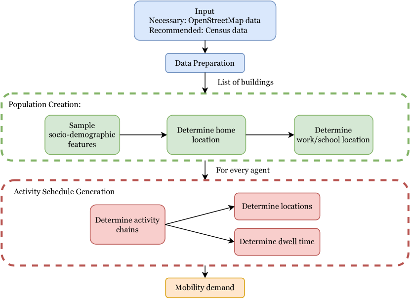
Figure 1: Architecture of OMOD

The following section will describe OMOD’s architecture and the methodology that lead to the default parameterization. The parameterization process of each model step is explained directly after its description.

The mobility demand generation process consists of three steps. The first step is creating a model of the user-specified area (see Section 3.1). This step involves parsing the OSM file into a list of locations where activities can be conducted. The second step is the creation of the population (see Section 3.2). Here, the agents are assigned socio-demographic features, and their inflexible locations (home, school, workplace) are determined. The third and last step handles the activity schedule generation (see Section 3.3). Here, the model determines what activities, where, and for how long every agent conducts on a given day. This is the most complex step and takes up most of OMOD’s runtime.

Figure 1 depicts a high-level overview of OMOD’s architecture.

3.1 Data Preparation

The data preparation process parses the OSM file and combines it with optional census data to create a list of building instances characterized by the features depicted in Table 1.

Features:
coordinates
area
population
landuse
number of shops
number of offices
number of schools
number of universities
In focus area?

Table 1: Building features determined in the data preparation step. These features are parsed from the OSM input data, except for population, which is parsed from census data.

Firstly, OMOD determines the geometry of the area of interest (from here on called focus area) from a user-specified GeoJSON file. Since people living in the immediate surrounding often significantly impact the mobility demand in the area of interest, it is good practice to model the surrounding as well [27]. For this purpose, OMOD implements the option to buffer the focus area by a given distance. From here on, the additional area created this way will be called buffer area. Figure 2 shows an example of the area definition process.

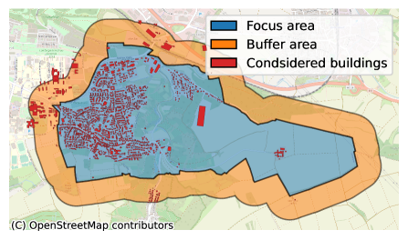
Figure 2: Example focus and buffer area in OMOD. Depicted is Gerbrunn in Germany (OSM id: 163738), with a buffer distance of $500\text{\,}\mathrm{m}$.

Once the area is defined, OMOD parses all OSM objects that intersect that area, utilizing the Osmosis tool. Objects with the building tag are added to the building list. The coordinates and area of each building are directly computed from the OSM objects. The remaining features are determined by combining the geometry information of each building with other OSM information in the following manner:

To determine the land use feature, we check whether each building intersects with a land use zone in the OSM data. The land use of the building is then that of the intersecting land use zone or none, if none intersects. Four land use classes are considered: residential, industrial, commercial, and none. Residential and industrial are equivalent to the respective OSM land use values. Commercial combines the OSM land use values commercial and retail. None represents all other possible values in OSM and no specified land use.

We determine the features number-of-shops and number-of-offices by counting the intersecting OSM objects with the tag shop or office. Similarly, the attributes number-of-schools and number-of-universities are determined by counting the intersecting OSM objects where the amenity tag has the value school or university, respectively.

The population of each building is extracted from the optional census data. This data must be formatted as a GeoJSON file containing a list of geometries and their populations. For example, in Germany the Zensus 2011 [43] can be used, where the population is given on the level of $100\text{\,}{\mathrm{m}}^{2}$ cells. The population of each census geometry is distributed uniformly across all intersecting buildings. The population is assumed to be zero for buildings with no census data. If no census data file is provided, OMOD will not make assumptions about the number of inhabitants in each building.

3.2 Population Creation

The population creation step creates a user-specified number of agents and defines their invariable attributes. These include each agent’s home location, workplace, and socio-demographic features.

Socio-demographic features

First, the socio-demographic features are determined. For every agent, a set of categorical features is sampled from a user-provided distribution. If none is provided, the model defaults to setting the features to undefined. This can be understood as defining the distribution to be the same as in the calibration survey.

It is assumed that one distribution of socio-demographic features is valid for the entire modeled area (i.e., the socio-demographic makeup of the population does not differ significantly from district to district.). The socio-demographic features considered by OMOD are:

• Age. Possible values: {0-40, 40-60, 60-100, or undefined}

• Homogenous group. Possible values: {working adult, non-working adult, student, or undefined}

• Mobility group. Possible values: {full car user, mixed car user, no car user, or undefined}

These socio-demographic categories are chosen based on the analysis of Schlund [40] and Joubert et al. [44], who determined that these features have the largest explanatory value for the mobility demand patterns observed in Germany and South Africa. We use this somewhat limited number of categories because our approach for dwell time estimation (further explained in Section 3.3.2) needs a sufficient number of samples for every combination of socio-demographic features. With an increasing number of features, combinations increases exponentially, and the maximum number of features that can be included is quickly reached.

Home location

Each agent’s home location is sampled from the list of buildings obtained in the data preparation step ($Buildings$). The probability that building ($i$) is the home location of the agent is the population of the building ($POP_{i}$) divided by the total population in the modeled area:

$$P(i=HOME)=\frac{POP_{i}}{\sum\limits_{\forall j\in Buildings}{POP_{j}}}$$ (1)

If no census data is provided, the home location is determined using the destination choice model of OMOD (see Section 3.3.3).

Work/School location

The work and school location sampling process depends on the realization of the home location. With a given home location, we determine the workplace/school location with a multinomial logit model (MNL) [45] that will also be used to choose flexible destinations (such as shopping locations). The exact methodology will be explained in Section 3.3.3. Broadly speaking, the model follows a disaggregated gravity model approach as described in [27]. The model comprises an attraction value estimated from building properties (see Table 1) and a deterrence function based on the distance between the workplace/school and the home location.

3.3 Activity Schedule Generation

⬇ "activities": [ { "type": "HOME", "stayTime": 327.073, "lat": 53.6157, "lon": 10.1072, "inFocusArea": true }, { "type": "WORK", "stayTime": 591.966, "lat": 53.5256, "lon": 9.8951, "inFocusArea": true }, { "type": "HOME", "stayTime": null, "lat": 53.6157, "lon": 10.1072, "inFocusArea": true }

Figure 3: Example of an activity schedule produced by the activity schedule generation step. type states the activity category. stayTime describes how long (in minutes) the agent stays at the activity. lat and lon indicate the location. inFocusArea states whether the activity was conducted inside the focus or buffer area (see Figure 2).

The mobility demand generation step produces daily activity schedules for every agent in the population. These schedules specify the number of activities the agent conducts on the day in question, as well as their category, location, and duration (dwell time). An example of such a schedule is depicted in Figure 3.

OMOD first samples a chain of activities. Then, the dwell times and locations are determined conditionally on the outcome but independently of each other.

OMOD uses a data-based approach to determine the activity chain and dwell times. This simplifies the modeling process compared to traditional MNL models but limits number of socio-demographic features that can be included. The destination choice model is implemented as a disaggregated gravity model (framed as an MNL). Therefore, it is easily expandable with additional explanatory features.

The activity schedule generation is calibrated with the German household travel survey MiD [21]. The MiD is a large-scale reoccurring household travel survey published by the Federal Ministry of Digital and Transport. We utilize the survey conducted in the year 2017. This survey is distributed in the form of four data sets that differ based on spatial resolution and the level of detail of personal information. For privacy preservation, the dataset with the highest spatial resolution contains the least detailed personal information and vice versa. Of these datasets, we utilize the data set B3 with the highest spatial resolution but the least detailed personal information. This data set contains information from about 300,000 respondents from 150,000 households. For each respondent, the data set includes socio-demographic features, access to different mobility options, place of residence, and a trip diary for one day in 2017. In total, the dataset includes 1,000,000 trips. For 500,000 of these, the start and stop locations are known with a resolution of $5km^{2}$, and for 100,000 with the highest resolution of $500m^{2}$.

3.3.1 Activity Chain

The first step of the activity schedule generation process is sampling each agent’s daily activity chain. An activity chain describes the sequence of activities an agent undertakes on a given day. For example, the chain $(home,\allowbreak work,\allowbreak shopping,\allowbreak home)$ states that the agent started his day at home, went to work, then went shopping, and, finally, returned home. Possible activity categories are home, work, school, shopping, and other.

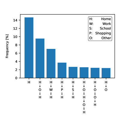
Figure 4: Empirical distribution of daily activity chains for an agent with undefined socio-demographic features and for an undefined weekday. For visual clarity, only the eight most common chains are depicted.

We sample these activity chains directly from empirical distributions. These are obtained by first filtering the MiD for each socio-demographic feature and weekday combination and then calculating the probability of each activity chain based on its frequency in the filtered dataset. An example of such a distribution is depicted in Figure 4 for the case where all socio-demographic features and the weekday are undefined.

For certain combinations of socio-demographic features, only a few samples exist. For example, students above the age of 60 are uncommon. Therefore, we must ensure that the empirical distributions are based on adequate sample sizes. We handle this issue by introducing a threshold for the minimum number of samples in the distribution. The threshold is set to 30, based on the common rule of thumb [46]. If a distribution has a smaller sample size than this threshold, we set individual socio-demographic features, or the weekday, to undefined until an adequate sample size is reached. This is done in the following order:

$$Age\rightarrow Mobility\ group\rightarrow Homogenous\ group\rightarrow weekday$$

I.e., first, the age is set to undefined; then, if the new distribution based upon this less restrictive set of conditions also has too few samples, the mobility group is set to undefined, and so on. Since the entirely unrestricted distribution has enough samples, this process will always return a distribution with adequate sample size.

The same threshold is applied to the minimum size of each activity chain. This is necessary because later on, for each activity chain, a distribution of dwell times is created (see Section 3.3.2) that again needs an adequate sample size. If an activity chain does not have the necessary sample size, it is removed from the empirical distribution. Approximately 10% of the samples must be discarded through this process. After the removal, OMOD includes 560 unique activity chains. The longest remaining chains consist of up to 14 consecutive activities.

Since longer activity chains are more complex, they are less likely to have enough samples, causing an underestimation of the number of daily trips. To combat this problem the probabilities of each activity chain are calibrated so that the total probability of all chains with a given length is equal to the probability of that length-group in the original dataset.

For consecutive days, an additional condition on the distribution is that each day must start with the same activity the previous day ended with. The first activity of the next day represents a continuation of the day’s last activity.

3.3.2 Dwell Time

With the activity chain for each agent determined, the time they spend on them can be sampled.

Similar to the process of activity chain sampling, the dwell times are sampled from distributions fitted to the MiD’s subset where the corresponding socio-demographic features and weekday are present. In this case, however, the subset depends not only on the combination of socio-demographic features and weekday but also on the specific activity chain. In other words, one distribution exists for each socio-demographic feature, weekday, and activity chain combination.

Previous work often chose methodologies where the dwell times of activities are sampled conditionally only on the dwell times at prior activities and not subsequent ones [40, 42]. This underestimates how holistically individuals plan their entire day. To combat this issue, OMOD samples dwell times from a multidimensional distribution, where each dimension encodes an activity of the activity chain. This way, all dwell times are sampled conjointly, and the temporal information of each daily activity schedule is coherent. This multidimensional distribution is modeled as a Gaussian Mixture.

For each feature combination we filter the MiD’s accordingly and fit a Gaussian Mixture to the filtered dataset using the scikit-learn python library. The number of Gaussians/components in the mixture is determined by increasing the number of components until the Bayesian Information Criterion score stops decreasing.

The MiD does not specify when the last activity of a day ends. We address this missing information by assuming that it lasts until midnight. Therefore, the dwell time at the last activity is wholly determined by those of the other activities, reducing the dimensionality of each mixture by one. In the rare case that the last activity begins after midnight, its duration is zero.

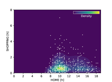
(a) Activity chain: (home → shopping → home)

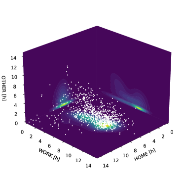
(b) Activity chain: (home → work → other → home)

Figure 5: Fitted Gaussian Mixture representing the dwell time distribution of two example activity chains with undefined socio-demographic features on an undefined weekday. The contours represent the density of the mixture projected onto each axis, where brighter colors represent a higher likelihood. The white points represent the records of the household travel survey (MiD). For visual clarity, only a fraction of the records are depicted.

Figure 5 shows examples of Gaussian Mixtures resulting from the described process. For example, the Gaussian depicted in Figure 5(a) describes the probability distribution for dwell times in the H→S→H chain. A likely sample drawn from this distribution would be [10.5, 1.3], meaning that the agent in question stays at home for 10.5 hours (i.e. until 10:30 AM), then goes shopping for 1.3 hours, and finally stayes at home again for the remainder of the day.

3.3.3 Destination Choice

The destination choice step determines where agents conduct activities. OMODs method for destination choice is based on the gravity model concept described by Ortuzar and Willumsen [27]. However, there are two key differences.

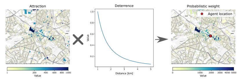
Figure 6: Destination choice: Architecture of the disaggregated gravity model.

Firstly, instead of aggregated traffic assignment zones, the set of possible destinations comprises all buildings in the focus and buffer area. Each time an agent has to choose a destination, the entire set is considered. Secondly, OMOD can not rely on aggregated origin-destination information like [27] because the user is not required to provide survey data. Therefore, we have to substitute this information. This is done with the attraction value $A_{i}$. The attraction governs the probability that a building is chosen when the agent’s location is taken into account. It can be seen as the suitability of a building for a given purpose. OMOD determines this value based on land use and POI information. For example, a building is more suitable for shopping if it contains shops. Consequently, a building with shops has a higher attraction value for shopping trips than one without. The distance to the building is factored into the decision process through a deterrence function $f(d)$ in the same manner as in [27].

All taken together, the following equation describes the probability that building $i$ is chosen as the destination:

$$P(i)=\frac{A_{i}\cdot f(d_{x,i})}{\sum\limits_{\forall j\in Buildings}{A_{j}\cdot f(d_{x,j})}}$$ (2)

or equivalently framed as an MNL:

$$P(i)=\frac{e^{V_{x,i}}}{\sum\limits_{\forall j\in Buildings}{e^{V_{x,j}}}}$$ (3)

with

$$V_{x,i}=\ln(A_{i})+\ln(f(d_{x,i}))$$ (4)

The distance ($d_{x,i}$) is calculated in reference to $x$, which is either the home location when the fixed locations (workplace and school) are determined or the agent’s current location. This distance refers to the routed distance by car, calculated with the open-source router GraphHopper.

If the user provides no census data, the home location is also determined with this model. In that case, the value of the deterrence function is set to 1, and only the attraction value of each building is relevant.

The parameterization of the deterrence function and each building’s attraction depends on the activity conducted at the destination. We call this activity the purpose of the trip from here on. For example, a building has a different probability of being the agent’s workplace than being the destination of a shopping trip. The weekday and the socio-demographic group do not influence the deterrence function and attraction value.

We obtain the parameterization of deterrence function and attraction values with the MiD, utilizing the methodology described in the following paragraphs.

Attraction

The attraction of each building is estimated with the linear function depicted in Equation 5 as inputs serve several OSM features. They can be separated into two groups. The first group is comprised of the variables denoted by an $a$. This group combines the area and land use of a building. Depending on the land use, one of these variables equals the area of the building, while the others are zero. For example, if the building is in a residential area, $a_{Residential}$ equals the building’s area and $a_{Industrial}$, $a_{Commercial}$, and $a_{Other}$ are zero. The second group comprises the variables denoted by an $u$ and describes the number of POI associated with a building. These can be shops, offices, schools, and universities. Additionally, depending on the land use, either $u_{Residential}$, $u_{Industrial}$, $u_{Commercial}$, or $u_{Other}$ equals one and the others zero.

$$A_{i}= \ 1+\theta_{0}\cdot a_{Residential}+\theta_{1}\cdot a_{Industrial}+\theta_{2}\cdot a_{Commercial}+$$ (5)

$$\ \theta_{3}\cdot a_{Other}+\theta_{4}\cdot u_{Office}+\theta_{5}\cdot u_{Shops}+$$

$$\ \theta_{6}\cdot u_{Schools}+\theta_{7}\cdot u_{Universities}+\theta_{8}\cdot u_{Residential}+$$

$$\ \theta_{9}\cdot u_{Industrial}+\theta_{10}\cdot u_{Commercial}+\theta_{11}\cdot u_{Other}$$

We determine the coefficients $\theta_{k}$ ($k\in\{0,1,...,11\}$) of Equation 5 through maximum likelihood estimation. The attraction value $A_{i}$ describes the probabilistic weight that a building $i$ is the destination for a trip under the condition that the agent’s location is unknown. Therefore, the probability that a trip with an unknown origin ends at building $i$ is:

$$P(i)=\frac{A_{i}}{\sum\limits_{\forall j\in Buildings}{A_{j}}}$$ (6)

The set Buildings describes all possible locations that an agent could have chosen as a destination. Since the MiD is a Germany-wide study, Buildings is comprised of all buildings in Germany. However, the MiD only specifies trip destinations at a resolution of $500\text{\,}{\mathrm{m}}^{2}$. Therefore, we aggregate all the features in Equation 5 on the level of the $500\text{\,}{\mathrm{m}}^{2}$ cells and consider all of these cells as suitable destination choices. This aggregation is possible due to the linearity of the attraction equation.

With the choice set defined, we can find the parameters $\theta_{k}$ of Equation 5 that maximize the probability of the observed trip destinations in the MiD for the trip purpose. The L-BFGS-B solver implementation of the python package SciPy is used to determine the maximum of the likelihood function.

We set the lower bounds of $\theta_{k}$ to zero. This means that each OSM feature can only attract but never deter. The introduction of these bounds has two main benefits. Firstly, they ensure that Equation 6 always yields positive non-zero probabilities for every building. Secondly, they introduce a level of regularization to the model, reducing the number of variables.

We further reduce the number of features with the following methodology. First, we fit the model several times, each time using all features except one, meaning that the coefficient $\theta$ of one feature is fixed to zero. Then we compare the likelihood of these iterations and create a ranking of features based on how much their absence worsened the results. After that, we build a model with only the most important feature, then one with only the two most important features, and so on, until no significant increase in likelihood is observable. The last set of features that improved the model is then chosen.

Activity	$\theta_{0}$	$\theta_{4}$	$\theta_{5}$	$\theta_{6}$	$\theta_{7}$
home	0.0327	0	314.09	1679.18	0
work	0	727.14	280.69	611.39	0
school	0	339.04	132.36	2115.64	3061.74
shopping	0	0	348.44	0	0
other	0.0370	2789.23	2179.04	1966.55	0

Table 2: Coefficients of the attraction function. See Equation 5 for the OSM feature corresponding to each $\theta_{k}$. $\theta$s that are not shown are zero.

Table 2 shows the resulting $\theta_{k}$ for each trip purpose. Since a building without any features has a fixed probability weight of one, the results can be interpreted as how much more likely a building with a specific POI is compared to a generic building. For example, a building with a shop is 350 times more likely to be a shopping destination. Similarly, we can interpret the coefficients of the residential area variable ($\theta_{0}$), which states how the probability increases with the area of the building (unit: square meter).

The results indicate that primarily POI data increases the attraction of a building, suggesting that these features have higher explanatory value for predicting trip destinations. However, during the model creation phase, we tested several different architectures for the attraction function. Land use and area features were more important for many similarly well-performing iterations. Therefore, we can not definitively say which features are the most relevant. Presumably, the high correlations between features on the aggregation level of $500\text{\,}{\mathrm{m}}^{2}$ are responsible for the inconclusiveness of our results.

Some artifacts of the aggregation can still be seen in the results for the home activity, where shops and schools have a significant impact. Note that the model for the home purpose is only chosen in the absence of census data. These artifacts are the main reason for introducing the feature reduction processes described above. Overall, however, the coefficients take reasonable values. The school purpose in the MiD includes apprenticeships. Therefore, the non-zero coefficient of shops and offices is not unreasonable.

Deterrence function

For the parameterization of the deterrence function we evaluate the following functional forms for $f(d_{x,j})$:

exponential (E)	$f(d_{x,j})=exp(\beta d_{x,j})$
power & exp. (PE)	$f(d_{x,j})=d_{x,j}^{n}\cdot exp(\beta d_{x,j})$
lognormal (L)	$f(d_{x,j})=\frac{1}{d_{x,j}\sigma\sqrt{2\pi}}exp(-\frac{(ln(d_{x,j})-\mu)^{2}}{2\sigma^{2}})$
lognormal & exp. (LE)	$f(d_{x,j})=\frac{1}{d_{x,j}\sigma\sqrt{2\pi}}exp(-\frac{(ln(d_{x,j})-\mu)^{2}}{2\sigma^{2}})\cdot exp(\beta d_{x,j})$

The first two functional forms are commonly used in related work [27]. The lognormal form is evaluated because it closely resembles the trip distance distribution in the MiD. Finally, the combined lognormal and exponential distribution is an attempt to introduce better tail behavior to the lognormal functional form.

In Equation 3, the deterrence function always occurs inside a logarithm. Therefore, we can significantly simplify the parameterization step of the deterrence function by directly fitting the logarithm.

If we take the natural logarithm of the functional forms, we get:

E	$ln(f(d_{x,j}))=\beta d_{x,j}$
PE	$ln(f(d_{x,j}))=\beta d_{x,j}+nln(d_{x,j})$
L	$ln(f(d_{x,j}))=-\frac{1}{2\sigma^{2}}ln^{2}(d_{x,j})+(\frac{\mu}{\sigma^{2}}-1)ln(d_{x,j})+\frac{\mu^{2}}{2\sigma^{2}}-ln(\sigma\sqrt{2\pi})$
LE	$ln(f(d_{x,j}))=-\frac{1}{2\sigma^{2}}ln^{2}(d_{x,j})+(\frac{\mu}{\sigma^{2}}-1)ln(d_{x,j})+\frac{\mu^{2}}{2\sigma^{2}}-ln(\sigma\sqrt{2\pi})+\beta d_{x,j}$

If we disregard constant terms and aggregate the coefficients of each linear term to individual independent parameters, we get the following linear forms:

E	$ln(f(d_{x,j}))=\vartheta_{0}d_{x,j}$
PE	$ln(f(d_{x,j}))=\vartheta_{0}d_{x,j}+\vartheta_{1}ln(d_{x,j})$
L	$ln(f(d_{x,j}))=\vartheta_{0}ln^{2}(d_{x,j})+\vartheta_{1}ln(d_{x,j})$
LE	$ln(f(d_{x,j}))=\vartheta_{0}ln^{2}(d_{x,j})+\vartheta_{1}ln(d_{x,j})+\vartheta_{2}d_{x,j}$

These are less constraint versions of the original functional forms that are significantly easier to handle in the parameterization step.

For each functional form, we find the parameters that maximize the likelihood of trip destinations in the MiD, assuming that each destination’s probability is governed by Equation 3. The parameters of the attraction function are already determined in the previous step and assumed constant here.

Similar to the parameterization of the attraction function, we consider all buildings in Germany as possible destinations and have to aggregate their attraction to $500\text{\,}{\mathrm{m}}^{2}$ cells. Additionally, we need the distance between the trip’s origin and all possible destinations. We utilize GraphHopper to determine the routed distance (by car) between every cell centroid and every other cell centroid.

This routing computation is very time intensive; even then, we leverage the ShortestPathTree API of GraphHopper. Therefore, the distance matrix has to be precomputed and stored in memory to reach reasonable optimization times. However, the memory consumption would be unacceptable with a distance matrix of the size $(1.5\cdot 10^{6})^{2}$ (the number of $500\text{\,}{\mathrm{m}}^{2}$ cells in Germany squared). For this reason, three simplifications are necessary. Firstly, we only determine the distance between cells that enclose buildings, halving the number of cells. Secondly, we introduce a distance limit of $300\text{\,}\mathrm{km}$. If the routed distance between two cells is above this limit, we do not route. Instead, we substitute with a beeline calculation fast enough not to require precomputation. Thirdly, we digitize the distance information into the $50\text{\,}\mathrm{m}$ wide bins. The process of this digitization is described in more detail in A.

With these simplifications, all the necessary data needed for the maximum likelihood estimation can be stored in memory, and the optimal parameters of each functional form are determined. The functional form is chosen for each trip purpose where the trip distance distribution produced by Equation 3 is closest to that in the MiD. We use the Kolmogorov-Smirnov test to measure the goodness of fit.

Activity	Form	$\vartheta_{0}$	$\vartheta_{1}$	$\vartheta_{2}$
work	EP	-0.035	-0.919	-
school	LE	-0.235	-1.176	0.005
shopping	L	-0.215	-1.414	-
other	L	-0.180	-1.067	-

Table 3: Coefficients and functional forms of the deterrence function for each trip purpose (activity at destination). The unit of distance used in the functions is kilometer.

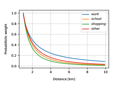
Figure 7: Values of the fitted deterrence functions $f(d_{x,j})$ over the distance from origin to destination.

The process results in the deterrence function parameterization depicted in Table 3. Figure 7 shows how the probabilistic weight of a destination falls over distance. We can see that the general shape of all deterrence functions is similar. However, the rate of decline differs significantly between purposes.

Grid

During runtime, Equation 3 has to be evaluated for every building in the model area each time an agent conducts an activity with no fixed location. This involves calculating the distance to every building and constitutes OMOD’s main performance bottleneck.

To speed up this process, we introduce a grid. When an agent makes a destination choice, first, the probability of each grid cell is determined using Equation 3, but with the aggregated attraction of all buildings within the grid cell and the distance from the agent to the centroid of these buildings. Subsequently, a cell is sampled, and the building inside it is chosen solely based on its attraction value, disregarding the distance differences of buildings within the same cell.

This grid can be defined in various ways. The naive approach is a regular grid where all grid cells are squares of equal size. However, since OMODs runtime rises quadratically with the number of cells (for every trip with a flexible location we have to calculate the distance from a cell to every other cell), it is advisable to introduce a more efficient grid. The error the grid introduces is characterized by the average distance between a building and the centroid representing its associated grid cell. This is the case because we calculate the distance from the origin only to the centroid of each cell, neglecting the positional deviation between the cell centroid and building location. Therefore, the best grid with $k$ cells is that where the sum of the within-cell variance of the building positions is smallest. We can find a suitable grid with the k-Means algorithm.

There are two problems with this approach. Firstly, the runtime of the standard k-Means algorithm is not insignificant (several minutes in our trials). Secondly, the number of cells should not be constant but increase with the size of the model area. We solve both of these issues by using the Bisecting-K-Means variant of the algorithm. This version results in a slightly higher within-cell variance but has significantly lower runtimes and has the added advantage that it can be implemented with a custom stopping criterion. Instead of stopping once we reach $k$ clusters/cells, we terminate the clustering algorithm once the average distance between each building and its associated centroid falls below a fixed threshold, representing the resolution of the grid. Per default, this threshold is $150\text{\,}\mathrm{m}$. In the subsequent validation, we use the default resolution for all tests. The resulting grid is depicted in Figure 8.

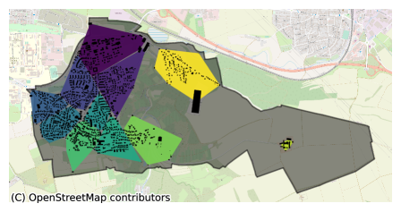
Figure 8: Example of the grid. Depicted is Gerbrunn, Germany (OSM id: 163738).

The presented grid creation process greatly reduces the necessary number of grid cells compared to a regular grid. Nonetheless, for large areas, the number of cells can quickly reach limits where the computation time becomes impractical. This issue is especially problematic since large buffer areas are often necessary to accurately recreate individuals’ daily driving distances. We combat this issue by reducing the grid resolution with the distance from the focus area, meaning that buildings far away from the original focus area are grouped into larger and larger cells. Specifically, we run the clustering approach described above separately for groups of buildings. The first group is all buildings in the focus area; the second is all buildings in the buffer area with a distance of fewer than $10\text{\,}\mathrm{km}$ to the focus area, then those between $10\text{\,}\mathrm{km}$ and $20\text{\,}\mathrm{km}$, and so on. We are doubling the grid resolution threshold for every new group of buildings. This way, we achieve adequate runtimes for large buffer radii.

4 Validation

We validate the model by determining how well the model reproduces the observations of the German household travel survey MiD [21]. First, we determine how close the spatial patterns of the mobility demand are reproduced. To do so, we compare how many trips each zone attracts, the origin-destination matrices, and the daily driven distances. Secondly, we analyze how well temporal patterns are reproduced by evaluating the share of persons that conduct a specific activity over the course of a week.

Please note that this validation is somewhat limited by the fact that the MiD is our primary source for calibration data. Therefore, the test and train sets are not strictly separated. However, regarding destination choice, we reduced the entire information of the MiD to the parameters described in Tables 2 and 3, in total, 24 non-zero parameters. Consequently, the risk of overfitting is reduced. The temporal characteristics have a significantly larger number of parameters that are also less explainable. However, the Gaussian Mixture methodology generally resulted in low numbers of Gaussians and the risk of overfitting to outliers is small. Regardless, the current parameterization of OMOD can only reproduce mobility behavior as observed in the MiD.

4.1 Spatial Validation

We evaluate the spatial model performance for three differently sized German cities. Kassel a smaller city with 200,000 inhabitants, the agglomeration area of Nuremberg with 1.3 million inhabitants, and Hamburg a large city with 2.5 million inhabitants. We chose these cities because of their populations and location (north, middle, and south).

Every city is simulated with 100,000 agents for four undefined days, using data from the German census of 2011 [43] to determine the distributions of home locations. The administrative boundary of each city defines the focus areas. Each focus area is buffered with a distance of $40\text{\,}\mathrm{km}$.

4.1.1 Zonal Trip Attraction

This test compares the trip destination distributions between the survey and model based on the share of trips that end in a given zone, where zones are cells of grids with $500\text{\,}\mathrm{m}$, $1\text{\,}\mathrm{km}$, and $5\text{\,}\mathrm{km}$ resolution (these grids are strictly for validation purposes and not to be confused with the grid used by OMOD internally). The results are depicted in Figure 9 for each focus area and with a resolution of $1\text{\,}\mathrm{km}$. In B, quantitive results are displayed for all resolutions.

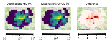
(a) Kassel

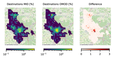
(b) Nuremberg

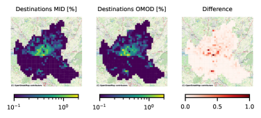
(c) Hamburg

Figure 9: Comparison of the share of trips that end in each $1\text{\,}\mathrm{km}$ cell between OMOD and the household travel survey MiD.

Qualitative results show that OMOD reproduces the overall popularity of different city districts for all three city sizes. This observation is supported by the high $R^{2}$ values of 0.87 to 0.95 on the lowest resolution level. For the medium resolution ($1\text{\,}\mathrm{km}$), the model’s performance decreases to 0.61-0.77 and, for the highest resolution ($500\text{\,}\mathrm{m}$), to 0.22-0.36. These reductions can be ascribed to the fact that predicting mobility demand with higher spatial resolution becomes increasingly difficult.

For each trip purpose, the results show similar performance and a similar performance decline for higher resolutions as in the overall case. The exception is home, where the performance declines significantly slower, reaching an $R^{2}$ value of 0.5 at the highest resolution. This result is unsurprising, as the validation uses census data with $100\text{\,}\mathrm{m}$ resolution. The remaining error is likely because of the six-year gap between the creation of the census and the household travel survey. If we do not use census information, we get $R^{2}$ values of 0.81-0.93 for the lowest resolution, with a similiar decline in performance at higher resolutions compared to the other purposes.

4.1.2 Origin-Destination Matrix

This test determines how well the origindestination matrix of the focus area is reproduced. We use the same methodology as in the trip attraction evaluation, only here, the probability distributions describe the probability that a trip starts in one cell and ends in another. While the first test determined whether the relative popularity of different parts of the city is well represented, this test determines whether the flows between city parts are realistic. We evaluate the $R^{2}$, the mean absolute error (MAE), and the Jensen-Shannon divergence between the flow distributions of the survey and model. The $500\text{\,}\mathrm{m}$ resolution level is not evaluated because, with an average number of 50 buildings per zone and more than 500 possible destinations (even for the smallest city), we enter the realm where we would need to predict the behavior of individuals, something that activity based models are incapable of [26]. The results are depicted in Table 4.

City	Resolution	$R^{2}$	MAE [%]	Jensen-Shannon
Kassel	$5\text{\,}\mathrm{km}$	0.956	0.211	0.134
	$1\text{\,}\mathrm{km}$	0.461	0.005	0.506
Nuremberg	$5\text{\,}\mathrm{km}$	0.715	0.044	0.174
	$1\text{\,}\mathrm{km}$	0.177	0.001	0.576
Hamburg	$5\text{\,}\mathrm{km}$	0.868	0.017	0.206
	$1\text{\,}\mathrm{km}$	0.025	0.000	0.626

Table 4: Origin-destination evaluation

For all cities the results on the $5\text{\,}\mathrm{km}$ resolution are good. This is promising as the origin-destination matrix has $n^{2}$ entrees, where $n$ is the number of grid cells. Therefore, it is significantely more complex than the trip destination distribution.

The model underperforms for Nuremberg, primarily because of a significant overestimation of trips that start and end in the city center. We can trace this back to a very high density of POI there. Possibly, at a certain density, the trip attraction increase of additional POI diminishes, suggesting that the attraction function could benefit from the addition of saturation effects.

The results on the $1\text{\,}\mathrm{km}$ resolution suffer from sample size issues. On this resolution, the survey contains one record for every five origin-destination pairs in Kassel, one for every twelve in Nuremberg, and one for every 33 in Hamburg. Nonetheless, even with limited samples, it seems clear that OMOD could perform better in this regard. Reproducing origin-destination matrices on this resolution is difficult, espacially if the model is not fine-tuned to the region in question. As a way forward, we suspect increasing the number of explanatory features by adding georeferenced census data in combination with more detailed socio-demographic features can lead to a significant performance increase. However, the core use case of OMOD should always utilize data available to anyone. Therefore, optimizing the model based on optional additional data sources has little priority. Another likely source of error is, neglecting congestion and modes other than the car (in particular public transportation) in the destination choice step, which is responsible for a significant misrepresentation of the generalized cost of travel for several origin-destination pairs. Implementing these into OMOD will be less problematic regarding ease of use because the GTFS format provides a good de facto standard for public transport timetables. However, an implementation poses significant runtime issues that need to be addressed.

4.1.3 Daily Driven Distance

Another crucial descriptive metric of mobility demand is the daily driven distance of individuals.

City	Metric	MiD	OMOD
Kassel	0.25-quantile	3.837	2.724
	Median	12.115	10.478
	0.75-quantile	25.650	21.797
	Mean	$21.869\pm 1.74$	$18.298\pm 0.06$
Nuremberg	0.25-quantile	4.200	3.040
	Median	13.320	12.200
	0.75-quantile	29.480	28.132
	Mean	$23.301\pm 0.90$	$20.668\pm 0.07$
Hamburg	0.25-quantile	4.900	3.684
	Median	14.400	16.228
	0.75-quantile	30.400	36.175
	Mean	$24.664\pm 0.78$	$24.990\pm 0.08$

Table 5: Daily kilometer comparison with a buffer distance of $40\text{\,}\mathrm{km}$

OMOD does not specify the route an agent takes from A to B. For the validation, we assign routes with an all-or-nothing approach, always choosing fastest route by car and disregarding congestion effects. This simple assignment strategy certainly comes with its own error that can not easily be separated from the error inherent to OMOD. The results are summarized in Table 5. Note that the MiD’s results do not include regular trips conducted during work (for example, if the person is a postman) or trips conducted while on vacation since OMOD does not model these kinds of trips.

We can see that for the largest city, the average daily kilometers are very closely reproduced. However, a slight overestimation of the variance occurs, meaning that short and long trips occur too often but in such a way that the average is preserved.

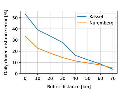
Figure 10: Dependency of the average daily driven distance error on the size of the buffer area.

For the smaller cities, we get an underestimation of the average daily kilometers. To some extent, this error is inevitable. Since only buildings included in the model can be destinations, the average daily distance can not exceed the average number of trips multiplied by the furthest distance in the model area. With an increased buffer area, the error should decrease. That indeed happens, as can be seen in Figure 10. With an increased buffer distance, the error for Nuremberg and Kassel falls to below $5\text{\,}\mathrm{\char 37\relax}$. The error could be reduced further. However, increasing the buffer area further is increasingly costly due to the quadratic increase in routing calculations that have to be done (see Section 3.3.3).

4.2 Temporal Validation

We have already ascertained the spatial validity of OMOD. Additionally, the model should reproduce the temporal patterns of real mobility demand. To validate this, we compare the share of agents conducting a specific activity at each point in time over a week in OMOD and the survey.

Some notes about our methodology: Firstly, since in OMOD, the first day for all agents begins at home, we simulate two weeks, the first to let the model settle and the second to use in the actual comparison. Secondly, trip assignment is conducted with the same all-or-nothing method as in Section 4.1.3.

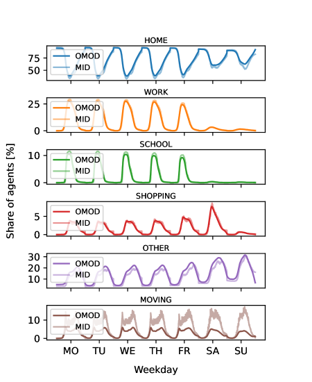
Figure 11: Temporal validation: Depicted is the share of agents conducting a specific activity over the course of a generic week in OMOD and the MiD household travel survey.

Figure 11 depicts the results. Overall, the temporal aspects of the mobility demand are very well reproduced. At no point did more than $13\text{\,}\mathrm{\char 37\relax}$ of the agents conduct the wrong activity. The average error over the timespan is $5\text{\,}\mathrm{\char 37\relax}$. This error is caused almost entirely by underestimating the number of moving agents, which can be traced back to the trip assignment process used in validation. In the all-or-nothing assignment process, all trips are conducted by car, only the pure driving duration is considered, and congestion effects are disregarded. On the other hand, the MiD includes all modes of transport, congestion effects, and inefficiencies like parking spot searches. Because of these factors, the all-or-nothing approach underestimates travel times, leading to an underestimation of moving agents and a corresponding overestimation at some other activity. Additionally, since OMOD does not specify fixed start times for activities the shorter travel times also mean that activities start and end earlier than they should, leading to a slight left shift of all activities that is corrected at the end of each day.

In the MiD time series, discontinuities are visible at midnight. These stem from the fact that each person is only questioned about one day from waking up to midnight. OMOD smooths these discontinuities out because it must remain self-consistent, leading to a discrepancy between the model and survey that should not be regarded as an error.

5 Runtime

OMODs runtime is mainly influenced by four components of the program. These are: parsing the OSM file, GraphHopper initialization, the routing matrix’s pre-computation, and the main simulation (where the simulation steps described in section 3.3 are run for all agents). In this section, we evaluate the runtime of each of these components for the focus area of Nuremberg, defined with the same boundaries as in Section 4. All tests are run on an ordinary scientific laptop (CPU: i7-1165G7 @ 2.8 GHz, RAM: 16 GB).

OSM file:
NUTS - Level	Name	OSM parsing	GraphHopper init
NUTS - 2	Middle Franconia	1min 10s	9s
NUTS - 1	Bavaria	1min 29s	1min 2s
NUTS - 0	Germany	3min 30s	6min 26s

Table 6: Runtimes of OSM parsing and GraphHopper initialization for differently sized OSM files.

The runtime of the first two components (OSM parsing and GraphHopper initialization) is dependent on the size of the OSM file. Table 6 depicts runtimes for OSM files of three differently sized regions encompassing the example city. The runtimes of these components are acceptable; OSM files of entire countries can be parsed in a reasonable time. The results are stored and reused for all subsequent runs of the same area.

Buffer dist.	Area size	Routing	Main Simulation. #Agents:
Unit: $km$	Unit: $km^{2}$	matrix init	$10^{3}$	$10^{4}$	$10^{5}$	$10^{6}$
0	$3.3\cdot 10^{2}$	2min 44s	1s	4s	29s	4min 56s
10	$1.7\cdot 10^{3}$	8min 42s	1s	4s	36s	6min 9s
20	$3.7\cdot 10^{3}$	17min 37s	1s	6s	42s	7min 16s
30	$6.2\cdot 10^{3}$	32min 50s	1s	6s	47s	7min 55s
40	$9.3\cdot 10^{3}$	52min 10s	2s	7s	49s	8min 27s

Table 7: Runtimes of routing matrix precomputation and the main simulation. The main simulation is the only component of the runtime that can not be stored and reused on subsequent runs.

As stated in Section 3.3.3, the main performance bottleneck of OMOD is repeatedly calculating the routed distance between an agent’s location and all possible destinations. For this reason, it is helpful to precompute the distances between all (or the most important) cells to all cells. We call this step the routing matrix precomputation. Precomputation simplifies the usage of the ShortestPathTree API of GraphHopper, as well as storing and reusing the results.

The runtime for precomputation of the routing matrix is depicted in Table 7. These runtimes depend on the size of the model area and, therefore, increase with the buffer radius. For large model areas the precomputation of the routing matrix requires significant time. In these cases, it is possible to reduce the spatial resolution of the routing grid (see Section 3.3.3) or switch the distance metric to the Euclidean Distance. Switching to the Euclidean Distance completely removes the need for precomputation, but doing so is only advisable for test runs, as it skews the results significantly.

The runtime of the main simulation increases linearly with the number of agents and days. Table 7 depicts the runtime of this component for one day and 1,000 to 1 million agents.

6 Conclusion

In this paper, we introduced the open-source mobility demand generator OMOD. OMOD determines activity schedules for a population of agents for a user-specified area of interest. These schedules state what an agent does, where, and for how long. The what and how long are sampled from probability distributions calibrated with household travel survey data. The where is determined with a disaggregated destination choice model inspired by the gravity model concept.

OMOD can be used in many different research fields, like communications research, energy system modeling, epidemiology, or for prototyping in transportation studies. For example, we use it in a publicly funded project [47] to determine the benefit of intelligent electric vehicle charging for operators of distribution grids.

We compare the generated mobility demand of OMOD to the results of the German household travel survey MiD. This validation led to the following conclusions:

• The trip destination distribution is satisfyingly reproduced for spatial resolutions up to $1\text{\,}\mathrm{km}$.

• Origin-destination matrices are significantly harder to reproduce. The results are satisfactory up to a resolution of $5\text{\,}\mathrm{km}$.

• The average daily driven distance error is negligible if the modeled area is large enough. For the best results we recommend an area of around $10\,000\text{\,}\mathrm{km}$.

• The share of agents conducting a specific activity at a each point in time matches the survey closely. The exception is the number of people currently moving. Here, a more sophisticated assignment process is necessary than the all-or-nothing approach used in our validation.

The validation uncovered several aspects in which the model could be improved. These include:

• The introduction of more explanatory variables. Especially spatially resolved socio-demographic features.

• The inclusion of non-linear effects of OpenStreetMap features on a location’s attractiveness.

• The inclusion of mode choice, public transportation, and congestion effects in the destination choice step.

• The inclusion of household interactions.

Including these aspects will likely necessitate the inclusion of more input data sources, such as more detailed census information and public transport schedules.

The biggest open question regards OMOD’s ability to translate to countries other than Germany. Technically, OMOD can be executed with a focus area that can be anywhere on Earth. However, the current parameterization is calibrated with German household travel survey data and has not yet been validated for other parts of the world. In future work, we aim to acquire mobility data for many more regions and will use it to evaluate and improve OMOD’s performance in as many places as possible.

Open-Source

OMOD is written in Kotlin (a modern JVM language) and is available on GitHub https://github.com/L-Strobel/omod under the MIT license. To execute the model, the user only needs to have Java installed on their machine, download an OpenStreetMap file of the area they are interested in, and define the focus area as a GeoJSON (for example, with https://geojson.io). See the GitHub page for a step-by-step description of how to run the model.

Appendix A Discrete Distance Destination Choice Function

In this section, we will explain how we reformulated the maximum likelihood problem described in Section 3.3.3 to reduce the memory costs by digitizing the distances into the set $D$ of discrete bins.

The original maximum log-likelihood problem is:

$$\underset{\theta}{arg\ max} \sum_{\forall(o,t)\in O}ln(P(o,t;\theta))$$ (7)

where $O$ is the set of all observed origin-destination pairs in the MiD data and $P((o,t);\theta)$ is the probability that the building $t$ is the destination of a trip starting at $o$:

$$P((o,t);\theta)=\frac{e^{\ln(A_{o})+\ln(f(d_{o,t};\theta))}}{\sum\limits_{\forall j\in Buildings}{e^{\ln(A_{j})+\ln(f(d_{o,j};\theta))}}}$$ (8)

If we reformulate Equation 7, we get:

$$\sum_{\forall(o,t)\in O}ln(A_{o})+ln(f(d_{o,t};\theta))-ln(\sum\limits_{\forall j\in Buildings}{A_{j}e^{\ln(f(d_{o,j};\theta))})}$$ (9)

Ignoring constant terms and introducing $B_{o,d}$ for the set of buildings that have the distance $d$ to the origin, we get:

$$\sum_{\forall(o,t)\in O}ln(f(d_{o,t};\theta))-ln(\sum\limits_{\forall d\in D}{(e^{\ln(f(d;\theta))}\sum\limits_{\forall j\in B_{o,d}}{A_{j}})})$$ (10)

Note, that the term $\sum\limits_{\forall j\in B_{o,d}}{A_{j}}$ does not depend on optimization variables $\theta$. Therefore, we can precalculate the term for all distances and observed origins before running the optimization. If we digitize the distances in $50\text{\,}\mathrm{m}$ wide bins, $D$ contains around $2\text{\times}{10}^{4}$ bins. Therefore, with the ${10}^{5}$ observations, we have to precompute and store $2\text{\times}{10}^{9}$ values, significantly less then the $9\text{\times}{10}^{10}$ values initially necessary for the distance matrix (with other simplifications already applied). The memory consumption of the other terms in Equation 10 is negligible. Therefore, this approach enables us to precompute and store all necessary information for the deterrence function parameterization in memory, making the fit on all of Germany possible.

Appendix B Zonal Trip Attraction Metrics

This section contains all the quantitive metrics that describe the similarity between the trip destination probability distributions in the MiD and that produced by OMOD.

Activity	Resolution	$R^{2}$	MAE [%]	Jensen-Shannon
All	$5\text{\,}\mathrm{km}$	0.935	1.692	0.073
All	$1\text{\,}\mathrm{km}$	0.769	0.289	0.210
All	$500\text{\,}\mathrm{m}$	0.215	0.162	0.407
home	$5\text{\,}\mathrm{km}$	0.849	2.472	0.139
home	$1\text{\,}\mathrm{km}$	0.728	0.341	0.236
home	$500\text{\,}\mathrm{m}$	0.513	0.171	0.408
work	$5\text{\,}\mathrm{km}$	0.993	0.859	0.073
work	$1\text{\,}\mathrm{km}$	0.646	0.479	0.326
work	$500\text{\,}\mathrm{m}$	0.114	0.225	0.532
shopping	$5\text{\,}\mathrm{km}$	0.820	2.673	0.142
shopping	$1\text{\,}\mathrm{km}$	0.565	0.478	0.333
shopping	$500\text{\,}\mathrm{m}$	-0.054	0.218	0.529
other	$5\text{\,}\mathrm{km}$	0.899	2.039	0.102
other	$1\text{\,}\mathrm{km}$	0.644	0.430	0.286
other	$500\text{\,}\mathrm{m}$	0.008	0.208	0.485
school	$5\text{\,}\mathrm{km}$	0.950	2.465	0.168
school	$1\text{\,}\mathrm{km}$	0.764	0.470	0.370
school	$500\text{\,}\mathrm{m}$	0.264	0.231	0.522

Table 8: Kassel: trip attraction metrics

Activity	Resolution	$R^{2}$	MAE [%]	Jensen-Shannon
All	$5\text{\,}\mathrm{km}$	0.874	0.739	0.090
All	$1\text{\,}\mathrm{km}$	0.641	0.104	0.215
All	$500\text{\,}\mathrm{m}$	0.290	0.051	0.388
home	$5\text{\,}\mathrm{km}$	0.927	0.745	0.092
home	$1\text{\,}\mathrm{km}$	0.796	0.100	0.215
home	$500\text{\,}\mathrm{m}$	0.576	0.053	0.398
work	$5\text{\,}\mathrm{km}$	0.909	1.064	0.134
work	$1\text{\,}\mathrm{km}$	0.524	0.167	0.333
work	$500\text{\,}\mathrm{m}$	0.169	0.068	0.490
shopping	$5\text{\,}\mathrm{km}$	0.792	1.125	0.148
shopping	$1\text{\,}\mathrm{km}$	0.299	0.210	0.372
shopping	$500\text{\,}\mathrm{m}$	0.052	0.078	0.535
other	$5\text{\,}\mathrm{km}$	0.862	0.937	0.122
other	$1\text{\,}\mathrm{km}$	0.529	0.145	0.291
other	$500\text{\,}\mathrm{m}$	0.145	0.062	0.447
school	$5\text{\,}\mathrm{km}$	0.866	1.175	0.204
school	$1\text{\,}\mathrm{km}$	0.533	0.209	0.421
school	$500\text{\,}\mathrm{m}$	0.142	0.089	0.590

Table 9: Nuremberg: trip attraction metrics

Activity	Resolution	$R^{2}$	MAE [%]	Jensen-Shannon
All	$5\text{\,}\mathrm{km}$	0.950	0.390	0.089
All	$1\text{\,}\mathrm{km}$	0.613	0.047	0.206
All	$500\text{\,}\mathrm{m}$	0.359	0.023	0.363
home	$5\text{\,}\mathrm{km}$	0.907	0.454	0.101
home	$1\text{\,}\mathrm{km}$	0.765	0.052	0.216
home	$500\text{\,}\mathrm{m}$	0.572	0.023	0.361
work	$5\text{\,}\mathrm{km}$	0.873	0.649	0.146
work	$1\text{\,}\mathrm{km}$	0.562	0.087	0.359
work	$500\text{\,}\mathrm{m}$	0.309	0.034	0.513
shopping	$5\text{\,}\mathrm{km}$	0.492	0.876	0.186
shopping	$1\text{\,}\mathrm{km}$	0.390	0.090	0.358
shopping	$500\text{\,}\mathrm{m}$	0.202	0.032	0.486
other	$5\text{\,}\mathrm{km}$	0.919	0.531	0.126
other	$1\text{\,}\mathrm{km}$	0.458	0.065	0.274
other	$500\text{\,}\mathrm{m}$	0.128	0.029	0.447
school	$5\text{\,}\mathrm{km}$	0.771	0.793	0.200
school	$1\text{\,}\mathrm{km}$	0.381	0.113	0.473
school	$500\text{\,}\mathrm{m}$	0.153	0.044	0.632

Table 10: Hamburg: trip attraction metrics

References

- [1] Yuchen Song, Dawei Li, Qi Cao, Min Yang, and Gang Ren. The whole day path planning problem incorporating mode chains modeling in the era of mobility as a service. Transportation Research Part C: Emerging Technologies, 132:103360, November 2021.
- [2] Michiel de Bok, Gerard de Jong, Jaap Baak, Eveline Helder, Cindy Puttemans, Kurt Verlinden, Dana Borremans, René Grispen, Joris Liebens, and Marthe Van Criekinge. A Population Simulator and Disaggregate Transport Demand Models for Flanders. Transportation Research Procedia, 8:168–180, January 2015.
- [3] H. Zhou, J. L. Dorsman, M. Mandjes, and M. Snelder. Sustainable mobility strategies and their impact: A case study using a multimodal activity based model. Case Studies on Transport Policy, 11:100945, March 2023.
- [4] Jiangtao Liu, Jee Eun Kang, Xuesong Zhou, and Ram Pendyala. Network-oriented household activity pattern problem for system optimization. Transportation Research Part C: Emerging Technologies, 94:250–269, September 2018.
- [5] Tri K. Nguyen, Nam H. Hoang, and Hai L. Vu. A unified activity-based framework for one-way car-sharing services in multi-modal transportation networks. Transportation Research Part E: Logistics and Transportation Review, 157:102551, January 2022.
- [6] Riccardo Iacobucci, Jonas Donhauser, Jan-Dirk Schmöcker, and Marco Pruckner. The demand potential of shared autonomous vehicles: A large-scale simulation using mobility survey data. Journal of Intelligent Transportation Systems, 0(0):1–22, May 2023.
- [7] Kriste Henson, Konstadinos Goulias, and Reginald Golledge. An assessment of activity-based modeling and simulation for applications in operational studies, disaster preparedness, and homeland security. Transportation Letters, 1(1):19–39, January 2009.
- [8] Navid Mahdizadeh Gharakhanlou and Navid Hooshangi. Spatio-temporal simulation of the novel coronavirus (COVID-19) outbreak using the agent-based modeling approach (case study: Urmia, Iran). Informatics in Medicine Unlocked, 20:100403, January 2020.
- [9] David B. Johnson and David A. Maltz. Dynamic Source Routing in Ad Hoc Wireless Networks. In Tomasz Imielinski and Henry F. Korth, editors, Mobile Computing, The Kluwer International Series in Engineering and Computer Science, pages 153–181. Springer US, Boston, MA, 1996.
- [10] Michael Seufert, Anika Schwind, Marco Waigand, and Tobias Hoßfeld. Potential Traffic Savings by Leveraging Proximity of Communication Groups in Mobile Messaging. In 2018 14th International Conference on Network and Service Management (CNSM), pages 177–183, November 2018.
- [11] Liang Zhou. Mobile Device-to-Device Video Distribution: Theory and Application. ACM Transactions on Multimedia Computing, Communications, and Applications, 12(3):38:1–38:23, March 2016.
- [12] Michael Niebisch, Daniel Pfaller, and Anatoli Djanatliev. CoDiPy: Performance Evaluation of Vehicular Cooperative Downloading in Python. In 2022 18th International Conference on Wireless and Mobile Computing, Networking and Communications (WiMob), pages 461–465, October 2022.
- [13] Marta C. Gonzalez, Cesar Hidalgo, and Albert-Laszlo Barabasi. Understanding Individual Human Mobility Patterns. Nature, 453:779–82, July 2008.
- [14] Chaoming Song, Zehui Qu, Nicholas Blumm, and Albert-László Barabási. Limits of Predictability in Human Mobility. Science, 327(5968):1018–1021, February 2010.
- [15] Global Electric Vehicle Outlook 2022. 2022.
- [16] Xiaohui Li, Zhenpo Wang, Lei Zhang, Fengchun Sun, Dingsong Cui, Christopher Hecht, Jan Figgener, and Dirk Uwe Sauer. Electric vehicle behavior modeling and applications in vehicle-grid integration: An overview. Energy, 268:126647, April 2023.
- [17] Leo Strobel, Jonas Schlund, and Marco Pruckner. Joint analysis of regional and national power system impacts of electric vehicles—A case study for Germany on the county level in 2030. Applied Energy, 315:118945, June 2022.
- [18] Riccardo Iacobucci, Marco Pruckner, and Jan-Dirk Schmoecker. A large scale simulation of the electricfication effects of SAVs. In Giannis Adamos Eftihia G. Nathanail, Nikolaos Gavanas, editor, Smart Energy for Smart Transport - Proceedings of the 6th Conference on Sustainable Urban Mobility, volume 1 of Lecture Notes in Intelligent Transportation and Infrastructure. Springer, 2023.
- [19] Pablo Alvarez Lopez, Michael Behrisch, Laura Bieker-Walz, Jakob Erdmann, Yun-Pang Flötteröd, Robert Hilbrich, Leonhard Lücken, Johannes Rummel, Peter Wagner, and Evamarie Wiessner. Microscopic Traffic Simulation using SUMO. In 2018 21st International Conference on Intelligent Transportation Systems (ITSC), pages 2575–2582, November 2018.
- [20] Andreas Horni, Kai Nagel, and Kay W. Axhausen. The Multi-Agent Transport Simulation MATSim. Ubiquity Press, August 2016.
- [21] Infas and Bundesministerium für Verkehr und digialte Infrastruktur. Mobilität in Deutschland 2017. http://www.mobilitaet-in-deutschland.de.
- [22] Eric J. Miller and Matthew J. Roorda. Prototype Model of Household Activity-Travel Scheduling. Transportation Research Record, 1831(1):114–121, January 2003.
- [23] Matthew J. Roorda, Eric J. Miller, and Khandker M. N. Habib. Validation of TASHA: A 24-h activity scheduling microsimulation model. Transportation Research Part A: Policy and Practice, 42(2):360–375, February 2008.
- [24] Mark Bradley, John L. Bowman, and Bruce Griesenbeck. SACSIM: An applied activity-based model system with fine-level spatial and temporal resolution. Journal of Choice Modelling, 3(1):5–31, 2010.
- [25] Ram M. Pendyala, Ryuichi Kitamura, Akira Kikuchi, Toshiyuki Yamamoto, and Satoshi Fujii. Florida Activity Mobility Simulator: Overview and Preliminary Validation Results. Transportation Research Record, 1921(1):123–130, January 2005.
- [26] William Davidson, Robert Donnelly, Peter Vovsha, Joel Freedman, Steve Ruegg, Jim Hicks, Joe Castiglione, and Rosella Picado. Synthesis of first practices and operational research approaches in activity-based travel demand modeling. Transportation Research Part A: Policy and Practice, 41(5):464–488, June 2007.
- [27] Juan de Dios Ortúzar and Luis G. Willumsen. Modelling Transport, 4th Edition. Wiley, 2011.
- [28] Yoram Shiftan and Moshe Ben-Akiva. A practical policy-sensitive, activity-based, travel-demand model. The Annals of Regional Science, 47(3):517–541, December 2011.
- [29] Chandra R. Bhat, Jessica Y. Guo, Sivaramakrishnan Srinivasan, and Aruna Sivakumar. A Comprehensive Econometric Microsimulator for Daily Activity-Travel Patterns. Transportation Research Record, 1894:57–66, 2004.
- [30] Tom Bellemans, Bruno Kochan, Davy Janssens, Geert Wets, Theo Arentze, and Harry Timmermans. Implementation Framework and Development Trajectory of FEATHERS Activity-Based Simulation Platform. Transportation Research Record, 2175(1):111–119, January 2010.
- [31] Serio Agriesti, Claudio Roncoli, and Bat-hen Nahmias-Biran. Assignment of a Synthetic Population for Activity-Based Modeling Employing Publicly Available Data. ISPRS International Journal of Geo-Information, 11(2):148, February 2022.
- [32] Samuel Felbermair, Florian Lammer, Eva Trausinger-Binder, and Cornelia Hebenstreit. Generating synthetic population with activity chains as agent-based model input using statistical raster census data. Procedia Computer Science, 170:273–280, January 2020.
- [33] Sebastian Hörl and Milos Balac. Synthetic population and travel demand for Paris and Île-de-France based on open and publicly available data. Transportation Research Part C: Emerging Technologies, 130:103291, September 2021.
- [34] Sibren Isaacman, Richard Becker, Ramón Cáceres, Margaret Martonosi, James Rowland, Alexander Varshavsky, and Walter Willinger. Human mobility modeling at metropolitan scales. In Proceedings of the 10th International Conference on Mobile Systems, Applications, and Services, MobiSys ’12, pages 239–252, New York, NY, USA, June 2012. Association for Computing Machinery.
- [35] Darakhshan J. Mir, Sibren Isaacman, Ramon Caceres, Margaret Martonosi, and Rebecca N. Wright. DP-WHERE: Differentially private modeling of human mobility. In 2013 IEEE International Conference on Big Data, pages 580–588, Silicon Valley, CA, USA, October 2013. IEEE.
- [36] Kamil Smolak, Witold Rohm, Krzysztof Knop, and Katarzyna Siła-Nowicka. Population mobility modelling for mobility data simulation. Computers, Environment and Urban Systems, 84:101526, November 2020.
- [37] Kwang Sub Lee, Jin Ki Eom, and Dae-seop Moon. Applications of TRANSIMS in Transportation: A Literature Review. Procedia Computer Science, 32:769–773, January 2014.
- [38] Joerg Schweizer, Federico Rupi, Francesco Filippi, and Cristian Poliziani. Generating activity based, multi-modal travel demand for SUMO. In SUMO 2018- Simulating Autonomous and Intermodal Transport Systems, pages 118–101.
- [39] Lara Codeca, Jakob Erdmann, Vinny Cahill, and Jerome Haerri. SAGA: An Activity-based Multi-modal Mobility ScenarioGenerator for SUMO. SUMO Conference Proceedings, 1:39–58, 2020.
- [40] Jonas Schlund. Electric Vehicle Charging Flexibility for Ancillary Services in the German Electrical Power System. PhD thesis, Friedrich-Alexander-Universität Erlangen-Nürnberg, 2021.
- [41] Niklas Wulff, Fabia Miorelli, Hans Christian Gils, and Patrick Jochem. Vehicle Energy Consumption in Python (VencoPy): Presenting and Demonstrating an Open-Source Tool to Calculate Electric Vehicle Charging Flexibility. Energies, 14(14):4349, January 2021.
- [42] Carlos Gaete-Morales, Hendrik Kramer, Wolf-Peter Schill, and Alexander Zerrahn. An open tool for creating battery-electric vehicle time series from empirical data, emobpy. Scientific Data, 8(1):152, June 2021.
- [43] Statistische Ämter des Bundes und der Länder. Zensus 2011. www.zensus2011.de, 2011.
- [44] Johan W. Joubert and Alta de Waal. Activity-based travel demand generation using Bayesian networks. Transportation Research Part C: Emerging Technologies, 120:102804, November 2020.
- [45] Daniel McFadden. Conditional logit analysis of qualitative choice behavior. Frontier in Econometrics, 1973.
- [46] Robert V. Hogg and Elliot A. Tanis. Probability and Statistical Inference. Prentice Hall, 2006.
- [47] Model project ESM-Regio: Optimization of the energy system via sector coupling. https://www.bayern- innovativ.de/de/seite/esm-regio-en.