Estimation with ultimate quantum precision of the transverse displacement between two photons via two-photon interference sampling measurements

Abstract

We present a quantum sensing scheme achieving the ultimate quantum sensitivity in the estimation of the transverse displacement between two photons interfering at a balanced beam splitter, based on transverse-momentum sampling measurements at the output. This scheme can possibly lead to enhanced high-precision nanoscopic techniques, such as super-resolved single-molecule localization microscopy with quantum dots, by circumventing the requirements in standard direct imaging of cameras resolution at the diffraction limit, and of highly magnifying objectives. Interestingly, the ultimate spatial precision in nature is achieved irrespectively of the overlap of the two displaced photonic wavepackets. This opens a new research paradigm based on the interface between spatially resolved quantum interference and quantum-enhanced spatial sensitivity.

The Hong-Ou-Mandel (HOM) effect Hong et al. (1987); Shih and Alley (1988) is an emblematic quantum phenomenon that proved to be instrumental for the development of novel quantum technologies Bouchard et al. (2021). When two identical photons impinge on the two faces of a balanced beam splitter, and photodetectors are employed at both the outputs, no coincidence detection is recorded, as the two photons always ’bunch’ in the same output channel. This is caused by the quantum interference occurring between the two possible, but indistinguishable paths undertaken by the two identical photons through the beam splitter. If instead some distinguishability between the photons is introduced, caused for example by a relative time delay, different polarizations or central frequencies, coincidence events can be observed, and the coincidence rate changes with the distinguishability between the photons Hong et al. (1987); Shih and Alley (1988); Bouchard et al. (2021). For this reason, HOM interferometry has been largely employed for high-precision measurements, e.g., of optical lengths and time delays Hong et al. (1987); Lyons et al. (2018); Chen et al. (2019), polarisations Harnchaiwat et al. (2020); Sgobba et al. (2023), and for quantum-enhanced imaging techniques, such as quantum optical coherence tomography Abouraddy et al. (2002); Nasr et al. (2009). Furthermore, the analysis of the bounds on the precision achievable in an estimation protocol given by the Cramér-Rao bound Cramér (1999); Rohatgi and Saleh (2000), and of the ultimate precision achievable in nature through the quantum Cramèr-Rao bound Helstrom (1969); Holevo (2011), has become a useful tool to determine the sensitivity of two-photon interferometry techniques for metrological applications Lyons et al. (2018); Scott et al. (2020); Fabre and Felicetti (2021); Johnson et al. (2023).

Interestingly, it has been recently shown that inner-variables resolved two-photon interference, in which two delayed or frequency-shifted photons impinging on the two faces of the beam splitter are detected by frequency- or time-resolving detectors respectively, circumvents the requirement of large overlap in the photonic wavepackets typical of HOM interferometry Legero et al. (2003, 2004); Tamma and Laibacher (2015); Jin et al. (2015); Yepiz-Graciano et al. (2020); Triggiani et al. (2023); Wang et al. (2018); Hiemstra et al. (2020); Prakash et al. (2021). Indeed, this technique allows us to observe beating, i.e. oscillations, in probabilities of coincidence and bunching of the two photons, with a period that is inversely proportional to the difference in the colours or in the incidence times at the beam splitter, hence preserving its sensitivity also in the case of non-overlapping wavepackets Triggiani et al. (2023). Another practical advantages of inner-variables resolved two-photon interference are the possibility to reconstruct the interference pattern without slow mechanical scannings Yepiz-Graciano et al. (2020).

Two-photon interference has also been performed in the spatial domain, i.e. while varying transversal properties of the two photonic wavepackets, for example slightly rotating the momentum of the photons before they interfere Ou and Mandel (1989); Kim et al. (2006), manipulating the spatial overlap between the photons Lee and van Exter (2006), or simultaneously introducing a temporal delay to observe spatio-temporal coherence properties of the two-photon state Lee and van Exter (2006); Devaux et al. (2020). Spatial HOM interferometry so far has mostly been employed to assess the spatial coherence of highly entangled photons, e.g., produced by spontaneous parametric down-conversion. However, to the best of our knowledge, the metrological potential of spatial two-photon interference for high precision imaging and sensing applications has not been investigated yet. A study in this direction is made even more compelling, for an experimental and technological point of view, due to the recent development of high-precision nanoscopic techniques that already employ single-photon emitters and single-photon cameras Hanne et al. (2015); Bruschini et al. (2019); Urban et al. (2021).

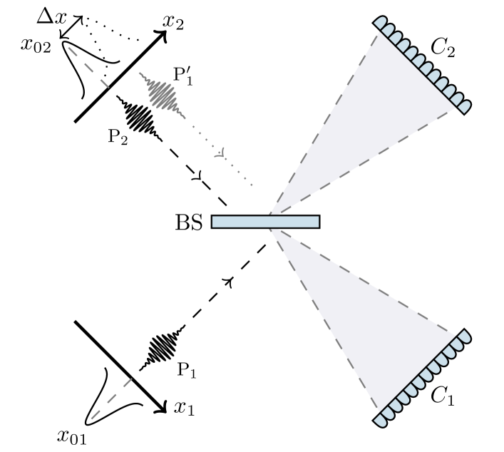
Figure 1: Two quasi-monochromatic photons, centred in positions $x_{01}$ and $x_{02}$ in their respective transverse planes, impinge onto the two faces of a balanced beam splitter (BS), so that the displacement between the probe photon $\mathrm{P}_{2}$ and the symmetric image $\mathrm{P}_{1}^{\prime}$ of the reference photon $\mathrm{P}_{1}$ is $\Delta x=x_{01}-x_{02}$. The two photons are then detected by two cameras ($C_{1}$ and $C_{2}$) in the far-field regime, which resolve their transverse momenta $k$ and $k^{\prime}$ for joint detections either in the same (bunching events) or opposite (coincidence events) output channels.

This work introduces a quantum interference technique based on spatially resolved sampling measurements, and investigates its properties from the metrological point of view. We show that resolving and sampling over the transverse momenta of two interfering photons, generated for example by a reference and a target single-photon emitter respectively, is an optimal metrological scheme for the estimation of the transverse separation of their wavepackets, achieving the ultimate precision given by the quantum Cramér-Rao bound. This can be done by employing two cameras that spatially sample over all the possible two-photon interference events in the far field, and simultaneously record whether the two photons ended up in the same or different output channels of the beam splitter (see Figure 1). This can therefore be seen as an interesting metrological application for spatial estimation of multiboson correlation sampling based on inner-variable sampling measurements Laibacher and Tamma (2015); Tamma and Laibacher (2016, 2023). In particular, we show that the precision achieved is independent of the separation between the spatial wavepackets of the two photons that we aim to estimate, which makes this technique relevant for localization and tracking applications. Furthermore, the precision of this scheme can be, in principle, increased arbitrarily, for any fixed displacement between the photons, by employing photons with broader and broader transverse-momentum distributions. Since our technique does not involve a direct detection of the single photons in the position domain, it removes the need of high-resolution cameras capable to directly resolve sources at the diffraction limit. As a result, this technique does not require in principle highly magnifying objectives, typically employed in super-resolution localization microscopy techniques, therefore decreasing the sources of aberration Ober et al. (2004); Lelek et al. (2021). Moreover, for the estimation of small separations of the two wavepackets, such that these are mostly overlapping, the resolving cameras can be replaced with bucket detectors that only count coincidences and bunching events, without affecting the sensitivity of the scheme. Other than single molecule localization nanoscopy, this technique finds possible applications in astrophysical bodies localization, or for the measurement of any transverse displacement of a probe single-photon beam with respect to a reference beam, e.g. caused by refraction or by optical devices such as tuneable beam displacers Salazar-Serrano et al. (2015).

Experimental setup.

We consider pairs of quasi-monochromatic photons, with wavenumber $k_{0}$, produced by two independent sources impinging on the two faces of a balanced beam-splitter, and then detected by two cameras positioned at the beam-splitter outputs in the far-field regime at a distance $d$ from their sources. For simplicity, we will only describe one transverse dimension of the setup, but the same analysis can be easily generalised to the two-dimensional case. We suppose that the transverse position of the $S$-th photon is described by a wavepacket $\psi_{S}(x)=\psi(x-x_{0,S})$ centred around the position $x_{0,S}$, with $S=1,2$. A practical example of such setup is shown in the schematic representation of Figure 1. We can thus write the two-photon state as

$$\ket{\Psi}=\int\mathrm{d}x_{1}\ \psi_{1}(x_{1})\hat{a}_{1}^{\dagger}(x_{1})\ket{0}_{1}\otimes\int\mathrm{d}x_{2}\ \psi_{2}(x_{2})\hat{a}_{2}^{\dagger}(x_{2})\ket{0}_{2},$$ (1)

where $\hat{a}^{\dagger}_{S}(x_{S})$, with $S=1,2$, is the bosonic creation operator associated with the $S$-th input mode of the beam-splitter at transverse position $x_{S}$, satisfying the commutation relation $\commutator{\hat{a}_{S}(x)}{\hat{a}^{\dagger}_{S^{\prime}}(x^{\prime})}=\delta_{SS^{\prime}}\delta(x-x^{\prime})$, where $\delta_{SS^{\prime}}$ and $\delta(x-x^{\prime})$ denote the Kronecker and Dirac delta respectively. For example, the displacement $\Delta x=x_{01}-x_{02}$ that we aim to measure can be caused by refraction or any other beam-displacing optical device Salazar-Serrano et al. (2015), or it can represent the position of a single-photon source that we want to localise, e.g. a probe quantum dot attached to a molecule Hanne et al. (2015); Bruschini et al. (2019); Urban et al. (2021), with respect to an identical reference photon emitted at a known position.

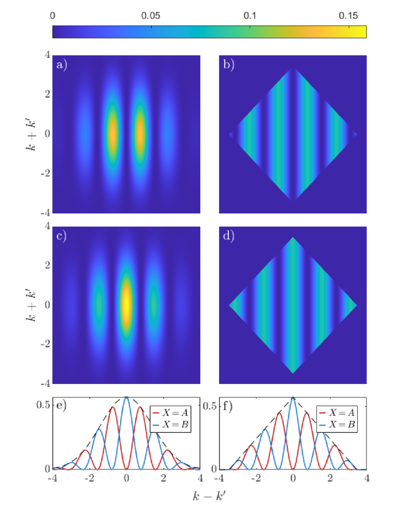
Figure 2: Examples of joint probability $P(k,k^{\prime},X)$ in Eq. (2) plotted along the axes $k-k^{\prime}$ and $k+k^{\prime}$ for two different transverse-momentum distributions $\absolutevalue{\varphi(k)}^{2}$, Gaussian on the left, a) and c), and rectangular on the right, b) and d). The plots a) and b) represent same-camera ($X=B$) detection probabilities, while c) and d) two-cameras ($X=A$) detection probabilities. The variance of the distribution $\absolutevalue{\varphi(k)}^{2}$ is set to $\sigma_{k}^{2}=1$, and it fixes a natural scale for the transverse momenta $k$ and $k^{\prime}$, and for the separation $\Delta x$, set to $\Delta x=4/\sigma_{k}$. Plots e) and f) show such probabilities, integrated in $k+k^{\prime}$.

After impinging on the beam-splitter, each pair of photons is randomly detected at the pixels in positions $y$ and $y^{\prime}$ either of a single or distinct cameras. Since the detection occurs in the far-field regime, it corresponds to resolving the transverse momenta $k=yk_{0}/d$ and $k^{\prime}=y^{\prime}k_{0}/d$ of the two photons, i.e. the conjugate variables to the photon transverse positions. This results in the observation of quantum beats (see Figure 2) with periodicity inversely proportional to $\Delta x=x_{0,1}-x_{0,2}$ in the joint probabilities

$$P(k,k^{\prime},X)=\frac{1}{2}\absolutevalue{\varphi(k)}^{2}\absolutevalue{\varphi(k^{\prime})}^{2}\left(1+\alpha(X)\cos((k-k^{\prime})\Delta x)\right),$$ (2)

of the two photons detected by different cameras ($X=A$), or the same camera ($X=B$), with momenta $k$ and $k^{\prime}$, where $\alpha(A)=-$ and $\alpha(B)=+$, and $\varphi$ denotes the Fourier transform of $\psi$, i.e. the transverse-momentum probability-amplitude distribution of the photons [SeeSupplementalMaterialat(URLwillbeinsertedbypublisher)forthederivationsof\lx@cref{creftypeplural~refnum}{eq:Prob}; \lx@cref{refnum}{eq:QFI}; \lx@cref{refnum}{eq:FIContr}; \lx@cref{refnum}{eq:FINRMain}and\lx@cref{refnum}{eq:FIABLarge}whichincludes\cite[cite]{\@@bibref{AuthorsPhrase1YearPhrase2}{Glauber1963}{\@@citephrase{(}}{\@@citephrase{)}}}]Suppl. The estimation is thus carried out by sampling the outcomes $(k,k^{\prime},X)$ from the probability in Eq. (2). In Eq. (2), we assumed that the size $\delta y$ of each pixel is small enough to sufficiently resolve the transverse-momentum distributions of the two photons and the beating oscillations, with period inversely proportional to $\Delta x$, i.e.

$$\delta y\ll\frac{d}{k_{0}}\sigma_{k},\quad\delta y\ll\frac{d}{k_{0}}\frac{1}{\Delta x},$$ (3)

where $\sigma_{k}^{2}$ is the variance of the transverse-momentum distribution of the photons. Noticeably, we will show that employing transverse-momentum distributions $\absolutevalue{\varphi(k)}^{2}$ with large variances is advisable, as they yield a better sensitivity. Since this technique requires cameras only able to resolve broad transverse-momentum distributions, and oscillations of period $\propto 1/\Delta x$, it circumvents the need to employ objectives with high magnifying factors to resolve directly the position of the single-photon emitters at the diffraction limit, typically required in imaging techniques such as single-molecule localization microscopy Ober et al. (2004); Lelek et al. (2021).

Ultimate quantum sensitivity.

Any unbiased estimator $\widetilde{\Delta x}$ associated with the estimation of a physical property, e.g. the separation $\Delta x$ between the photon pair in Eq. (1), has a variance $\mathrm{Var}[\widetilde{\Delta x}]$ that is bounded from below by quantum Cramér-Rao bound, which sets the ultimate quantum limit of the achievable precision in the estimation of $\Delta x$ Helstrom (1969); Paris (2009); Holevo (2011); Liu et al. (2019). At the same time, the precision achievable with a specific measurement scheme is also limited by a second lower bound, namely the (classical) Cramér-Rao bound Cramér (1999); Rohatgi and Saleh (2000). These bounds generate the chain of inequalities

$$\mathrm{Var}[\widetilde{\Delta x}]\geqslant\frac{1}{NF(\Delta x)}\geqslant\frac{1}{NH(\Delta x)},$$ (4)

where $H(\Delta x)$ is the quantum Fisher information, $F(\Delta x)$ the (classical) Fisher information, and $N$ is the number of independent repetitions of the measurement Cramér (1999); Helstrom (1969). Importantly, for a given measurement scheme, the first inequality in Eq. (4) can always be asymptotically saturated for large $N$ employing the maximum-likelihod estimation Cramér (1999); Rohatgi and Saleh (2000). Therefore, a measurement scheme is (asymptotically) optimal when the Fisher information associated with it equates the quantum Fisher information.

Indeed, we find out that our measurement scheme is optimal, and in particular

$$F(\Delta x)=H(\Delta x)=2\sigma^{2}_{k},$$ (5)

with the Fisher information directly proportional to the variance $\sigma_{k}^{2}$ of the transverse-momentum distribution $\absolutevalue{\varphi(k)}^{2}$ [SeeSupplementalMaterialat(URLwillbeinsertedbypublisher)forthederivationsof\lx@cref{creftypeplural~refnum}{eq:Prob}; \lx@cref{refnum}{eq:QFI}; \lx@cref{refnum}{eq:FIContr}; \lx@cref{refnum}{eq:FINRMain}and\lx@cref{refnum}{eq:FIABLarge}whichincludes\cite[cite]{\@@bibref{AuthorsPhrase1YearPhrase2}{Glauber1963}{\@@citephrase{(}}{\@@citephrase{)}}}]Suppl. Furthermore, a number of sampling measurements only of the order of $\sim 1000$ is enough to reach the desired sensitivity through maximum likelihood estimation, without the need of fully retrieving the output probability distribution with a large number of measurements Triggiani et al. (2023).

Remarkably, the ultimate precision expressed by the quantum Fisher information in Eq. (5) achieved with our technique is independent of the transverse separation $\Delta x$ between the two sources, regardless of the overlap of the two photons wavepackets in the space domain, and can be, in principle, arbitrarily increased by increasing the transverse-momentum variance $\sigma_{k}^{2}$ of the photons. Moreover, in addition to yielding a greater sensitivity, larger variances $\sigma_{k}^{2}$ in the transverse-momentum also reduce the resolution requirements in Eq. (3) so that magnifying objectives are not required.

Interestingly, this interferometric technique is completely unaffected by the lack of overlap between the spatial wavepackets of the two photons. Indeed, performing transverse-momentum resolving detections, i.e., resolving the variables in the conjugate domain to the position, renders the detectors “blind” to the position of emission of the two photons, and thus it enables the observation of two-photon quantum interference. This feature is in stark contrast with standard non-resolving two-photon interference, where the distinguishability of photons with non-overlapping wavepackets is not erased at the detectors, hindering the precision of the estimation [SeeSupplementalMaterialat(URLwillbeinsertedbypublisher)forthederivationsof\lx@cref{creftypeplural~refnum}{eq:Prob}; \lx@cref{refnum}{eq:QFI}; \lx@cref{refnum}{eq:FIContr}; \lx@cref{refnum}{eq:FINRMain}and\lx@cref{refnum}{eq:FIABLarge}whichincludes\cite[cite]{\@@bibref{AuthorsPhrase1YearPhrase2}{Glauber1963}{\@@citephrase{(}}{\@@citephrase{)}}}]Suppl.

Fisher information analysis.

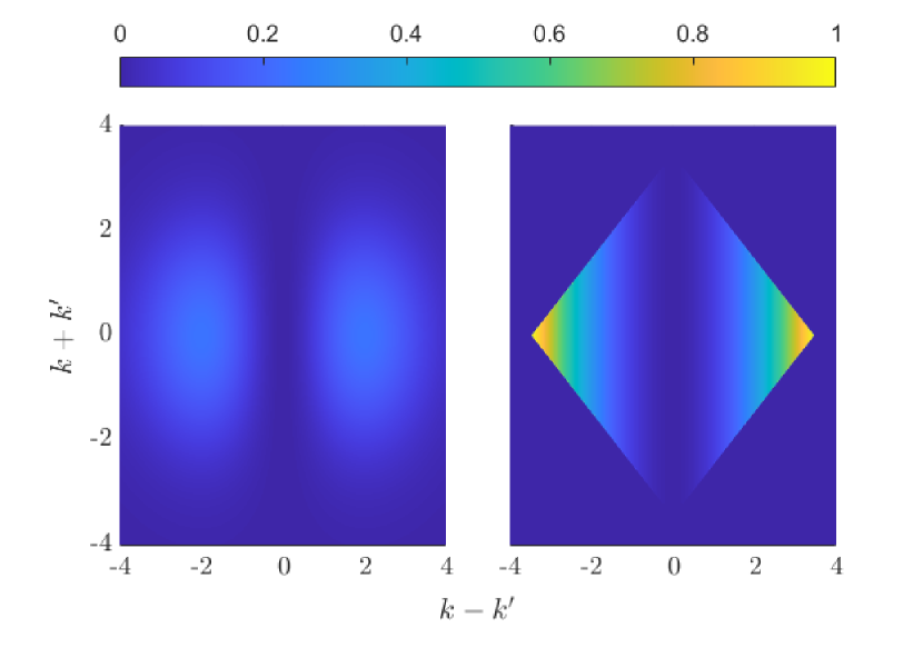
Figure 3: Sum $f(k,k^{\prime},A;\Delta x)+f(k,k^{\prime},B;\Delta x)$ of the contributions from the outcomes $(k,k^{\prime},A)$ and $(k,k^{\prime},B)$ to the Fisher information found in Eq. (7) for Gaussian (left) and uniform (right) transverse-momentum distributions $\absolutevalue{\varphi(k)}^{2}$ with unit variance $\sigma_{k}^{2}=1$, which fixes a natural unit for the transverse momenta $k$ and $k^{\prime}$. Most of the information on $\Delta x$ can be obtained by sampling measurements in the transverse momenta $k$ and $k^{\prime}$ only in a range of $\sim\!3\sigma_{k}$, and it is concentrated around two maxima at specific values of $k-k^{\prime}$. Noticeably, these plots are independent of $\Delta x$.

The Fisher information $F(\Delta x)$ in Eq. (5), whose outcomes $(k,k^{\prime},X)$ are governed by the probability distribution $P(k,k^{\prime},X)$ in Eq. (2), can be written as the sum

$$F(\Delta x)=\sum_{X=A,B}\int\mathrm{d}k\mathrm{d}k^{\prime}\ f(k,k^{\prime},X;\Delta x)$$ (6)

of the contributions

$$f(k,k^{\prime},X;\Delta x)=\frac{1}{2}\absolutevalue{\varphi(k)}^{2}\absolutevalue{\varphi(k^{\prime})}^{2}(k-k^{\prime})^{2}\\ \times(1-\alpha(X)\cos((k-k^{\prime})\Delta x)),$$ (7)

each one representing the information yielded by the outcome $(k,k^{\prime},X)$ of a single pair of photons [SeeSupplementalMaterialat(URLwillbeinsertedbypublisher)forthederivationsof\lx@cref{creftypeplural~refnum}{eq:Prob}; \lx@cref{refnum}{eq:QFI}; \lx@cref{refnum}{eq:FIContr}; \lx@cref{refnum}{eq:FINRMain}and\lx@cref{refnum}{eq:FIABLarge}whichincludes\cite[cite]{\@@bibref{AuthorsPhrase1YearPhrase2}{Glauber1963}{\@@citephrase{(}}{\@@citephrase{)}}}]Suppl. The expression of the contributions $f(k,k^{\prime},X;\Delta x)$ in Eq. (7) allows us to understand, of all the possible outcomes $(k,k^{\prime},X)$, which ones yield more information on the separation $\Delta x$, and conversely which ones are less informative and can be discarded with a negligible change of the overall precision. This type of analysis is useful from an experimental standpoint since, for example, it can help to choose efficiently the sensing range and the position of the two cameras.

In general, the term $f(k,k^{\prime},X;\Delta x)$ strongly depends on the shape of the transverse-momentum distribution $\absolutevalue{\varphi(k)}^{2}$, but some interesting universal properties of $f(k,k^{\prime},X;\Delta x)$ can be found. Firstly, the presence of the envelope $\absolutevalue{\varphi(k)}^{2}\absolutevalue{\varphi(k^{\prime})}^{2}(k-k^{\prime})^{2}$ as shown in Eq. (7) guarantees that, if the tails of the distribution $\absolutevalue{\varphi(k)}^{2}$ have negligible contribution (e.g. for distribution with finite support, or decreasing exponentially for large $k$), then it is possible to approximate the integration domain in Eq. (6) to a few units of $\sigma_{k}$ ($\sim 3\sigma_{k}$ for Gaussian and uniform transverse-momentum distributions), hence limiting the required cameras sensing range (see Figure 3). Noticeably, this envelope does not depend on the displacement $\Delta x$, meaning that the size of the cameras does not need to be adjusted according to the unknown separation between the two photons.

An interesting insight regarding the role of the two-camera ($X=A$) and same-camera ($X=B$) detection events in our transverse-momentum resolving technique is given by separately quantifying their overall contributions to the information on $\Delta x$. These contributions can be evaluated integrating the expression in Eq. (7) over all possible transverse momenta $k$ and $k^{\prime}$, obtaining

$$F(X;\Delta x)=\sigma_{k}^{2}-\frac{1}{2}\alpha(X)\Phi(\varphi;\Delta x),$$ (8)

with

$$\Phi(\varphi;\Delta x)=\int\mathrm{d}k\mathrm{d}k^{\prime}\ \absolutevalue{\varphi(k)}^{2}\absolutevalue{\varphi(k^{\prime})}^{2}(k-k^{\prime})^{2}\\ \times\cos((k-k^{\prime})\Delta x)).$$ (9)

From Eq. (8), we see that the same-camera and two-camera detection events contribute differently to the overall sensitivity, with the term $\Phi(\varphi;\Delta x)\equiv F(A,\Delta x)-F(B,\Delta x)$ quantifying the difference of the two contributions (see Figure 4).

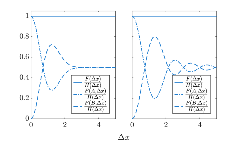
Figure 4: Plots of the Fisher information $F(\Delta x)$ in Eq. (5) (solid line), and of the contributions $F(A;\Delta x)$ (dash-dotted line) and $F(B;\Delta x)$ (dashed lined) in Eq. (8) from joint detection at both cameras $(X=A)$, and at a single camera $(X=B)$, normalised to $H(\Delta x)$, for Gaussian (left) and uniform (right) transverse-momentum distributions $\absolutevalue{\varphi(k)}^{2}$ with unit variance $\sigma_{k}^{2}=1$, which fixes a natural unit for $\Delta x$.

For small separations $\Delta x\ll 1/\sigma_{k}$, such that the spatial wavepackets are mostly overlapping, the difference $\Phi(\varphi;\Delta x\simeq 0)\simeq 2\sigma_{k}^{2}$ reaches its maximum value, therefore most of the information is obtained with joint detection events at both cameras. Interestingly, in this regime it is possible to replace, without any loss in sensitivity, the resolving cameras with simple bucket detectors, as the Fisher information

$$F^{\mathrm{(nr)}}(\Delta x)\simeq 2\sigma_{k}^{2}$$ (10)

associated with the detection of bunching and coincidence events without resolving the transverse momenta is approximately equal to the quantum Fisher information $H(\Delta x)$ [SeeSupplementalMaterialat(URLwillbeinsertedbypublisher)forthederivationsof\lx@cref{creftypeplural~refnum}{eq:Prob}; \lx@cref{refnum}{eq:QFI}; \lx@cref{refnum}{eq:FIContr}; \lx@cref{refnum}{eq:FINRMain}and\lx@cref{refnum}{eq:FIABLarge}whichincludes\cite[cite]{\@@bibref{AuthorsPhrase1YearPhrase2}{Glauber1963}{\@@citephrase{(}}{\@@citephrase{)}}}]Suppl.

In the opposite regime of large separations $\Delta x\gg 1/\sigma_{k}$, such that essentially the two spatial wavepacket do not overlap, the beating oscillations in Eq. (2), as well as the oscillations in Eq. (7), become increasingly fast. In this regime, if $\absolutevalue{\varphi(k)}^{2}$ is not highly concentrated around certain values of $k$, it can be considered essentially constant within every small interval $2\pi/\Delta x$ corresponding to one beating period. In this case, the integral $\Phi(\varphi,\Delta x)$ in Eq. (9) vanishes [SeeSupplementalMaterialat(URLwillbeinsertedbypublisher)forthederivationsof\lx@cref{creftypeplural~refnum}{eq:Prob}; \lx@cref{refnum}{eq:QFI}; \lx@cref{refnum}{eq:FIContr}; \lx@cref{refnum}{eq:FINRMain}and\lx@cref{refnum}{eq:FIABLarge}whichincludes\cite[cite]{\@@bibref{AuthorsPhrase1YearPhrase2}{Glauber1963}{\@@citephrase{(}}{\@@citephrase{)}}}]Suppl, and thus

$$F(A,\Delta x)=F(B,\Delta x)=\sigma_{k}^{2}.$$ (11)

Noticeably, since the two-camera and same-camera detection events yield the same amount of information for large $\Delta x$, it is possible to resolve only one of these two types of events, e.g. only the two-camera events, reducing the Fisher information by only a factor of two [SeeSupplementalMaterialat(URLwillbeinsertedbypublisher)forthederivationsof\lx@cref{creftypeplural~refnum}{eq:Prob}; \lx@cref{refnum}{eq:QFI}; \lx@cref{refnum}{eq:FIContr}; \lx@cref{refnum}{eq:FINRMain}and\lx@cref{refnum}{eq:FIABLarge}whichincludes\cite[cite]{\@@bibref{AuthorsPhrase1YearPhrase2}{Glauber1963}{\@@citephrase{(}}{\@@citephrase{)}}}]Suppl.

Conclusions.

We presented a spatial quantum interference technique allowing the estimation of the transverse separation of two single-photons beams at the ultimate precision allowed by the quantum Cramér-Rao bound, based on transverse-momentum resolved sampling measurements. We showed that the precision achieved with this technique is independent of the separation that we aim to measure, and it can be, in principle, arbitrarily increased by employing photons with more broadly distributed transverse momenta.

These features yield a number of important implications for experimental applications of our measurement technique. Firstly, despite its interferometric nature, this technique achieves the same precision irrespectively of the overlap between the two photonic wavepackets in the spatial domain. Indeed, resolving the transverse momenta erases the spatial distinguishability between the photons, allowing us to observe interference also in regimes where the separation is much larger than the spatial wavepackets widths. Secondly, the achieved ultimate precision is in principle unbounded, in the sense that is only limited by the highest value of the transverse-momentum distribution variance experimentally feasible with current technologies. Thirdly, by using indirect sampling measurements which resolve the photonic transverse momenta instead of the positions directly, this technique removes the requirement of cameras resolution at the diffraction limit typical of direct imaging techniques, as well as highly magnifying objectives, decreasing the sources of aberration. Furthermore, in the regime of transverse separation smaller than the spatial width of the wavepackets, the two cameras can even be replaced with non-resolving bucket detectors without any loss of sensitivity.

These results shed new light on the metrological power of two-photon spatial interference and can pave the way to new high-precision sensing techniques. This work has the potential to enhance super-resolution imaging techniques that already employ single-photon sources as probes for the localization and tracking of biological samples, such as single-molecule localization microscopy with quantum dots Hanne et al. (2015); Bruschini et al. (2019); Urban et al. (2021). Other possible applications can be found in the development of quantum sensing techniques for high-precision refractometry and astrophysical bodies localization. Finally, such a technique could, in principle, be also extended to the estimation of spatial parameters in a more general N-photon network by performing sampling measurements in the photonic transverse momenta.

Appendix A Joint detection probabilities in Eq. (2)

In this section we will evaluate the probability distribution $P(k,k^{\prime},X)$ in Eq. (2) in the main text associated with the event of detecting the two photons with transverse-momenta $k$ and $k^{\prime}$ in the same ($X=B$) and in different ($X=A$) cameras.

Since the detection occurs by means of cameras resolving the position of the photons in the far-field regime, we will first evaluate the second-order correlation functions Glauber (1963)

$$G^{(2)}_{CC^{\prime}}(y,y^{\prime})=\Tr[\outerproduct{\Psi}{\Psi}\hat{E}_{C}(y)\hat{E}_{C^{\prime}}(y^{\prime})\hat{E}^{+}_{C}(y)\hat{E}^{+}_{C^{\prime}}(y^{\prime})],$$ (12)

associated with the detection of the two photons at the pixels at the positions $y$ and $y^{\prime}$ of the cameras $C$ and $C^{\prime}$ respectively, with $C,C^{\prime}=C_{1},C_{2}$ and we denote with

$$\hat{E}^{+}_{C}(y)=\sum_{S=1,2}\int\mathrm{d}x_{S}\ g(x_{S},S;y,C)\hat{a}_{S}(x_{S})$$ (13)

the positive frequency part of the electric field operator at position $y$ of the camera $C$, with $\hat{E}^{-}_{C}(y)=(\hat{E}^{+}_{C}(y))^{\dagger}$ the negative frequency part, and

$$g(x,S;y,C)=\frac{\mathrm{e}^{\mathrm{i}\phi(S,C)}}{\sqrt{2}}\mathrm{e}^{\mathrm{i}k_{0}d}\mathrm{e}^{-\mathrm{i}\frac{k_{0}}{d}xy},$$ (14)

is the Fraunhofer transfer function, describing the propagation of the photon $S=1,2$ from transverse position $x$ through the beam-splitter and up to position $y$ at the detector $C=C_{1},C_{2}$ in the far-field, where $k_{0}$ is the wavenumber, $d$ is the longitudinal distance travelled by the photons to the detectors, $\phi$ is the phase acquired through the beam-splitter. In Eq. (14), we have chosen a dimensionless normalisation that guarantees the unitary propagation of the photons through the beam splitter.

To evaluate Eq. (12), we first introduce the electric field operators

$$\hat{E}_{SC}^{+}(y) =\int\mathrm{d}x_{S}\ g(x_{S},S;y,C)\hat{a}_{S}(x_{S}),\ S=1,2$$ (15)

associated with the $S$-th photon, so that

$$\hat{E}^{+}_{C}(y)=\sum_{S=1,2}\hat{E}^{+}_{SC}(y).$$ (16)

We can thus expand the second-order correlation function in Eq. (12) by employing Eq. (16), obtaining

$$G^{(2)}_{CC^{\prime}}(y,y^{\prime})=\sum_{\begin{subarray}{c}S_{1},S_{2}\\ S_{3},S_{4}\end{subarray}=1,2}\Tr[\outerproduct{\Psi}{\Psi}\hat{E}^{-}_{S_{1}C}(y)\hat{E}^{-}_{S_{2}C^{\prime}}(y^{\prime})\hat{E}^{+}_{S_{3}C}(y)\hat{E}^{+}_{S_{4}C^{\prime}}(y^{\prime})].$$ (17)

Of the 16 terms in the summation in Eq. (17), we easily see that only a few survive. Indeed, since the state $\ket{\Psi}$ has a single photon at each input channel, the terms with $S_{1}=S_{2}$ or $S_{3}=S_{4}$ vanish. Moreover, since the positive-frequency part of the electric field annihilates a photon, and the negative-frequency part creates a photon, evaluating the trace in Eq. (17) is equivalent to projecting onto the vacuum $\outerproduct{\mathrm{vac}}{\mathrm{vac}}$, so we have

$$G^{(2)}_{CC^{\prime}} (y,y^{\prime})=\sum_{S_{1},S_{3}=1,2}\matrixelement{\Psi}{\hat{E}^{-}_{S_{1}C}(y)\hat{E}^{-}_{\sigma(S_{1})C^{\prime}}(y^{\prime})}{\mathrm{vac}}$$

$$\quad\times\matrixelement{\mathrm{vac}}{\hat{E}^{+}_{S_{3}C}(y)\hat{E}^{+}_{\sigma(S_{3})C^{\prime}}(y^{\prime})}{\Psi},$$

$$=\absolutevalue{\sum_{S_{1}=1,2}\matrixelement{\mathrm{vac}}{\hat{E}^{+}_{S_{1}C}(y)\hat{E}^{+}_{\sigma(S_{1})C^{\prime}}(y^{\prime})}{\Psi}}^{2}$$ (18)

where $\sigma(1)=2,\sigma(2)=1$. We can now proceed with evaluating the scalar products in Eq. (18)

$$\matrixelement{\mathrm{vac}}{\hat{E}^{+}_{S_{1}C}(y)\hat{E}^{+}_{\sigma(S_{1})C^{\prime}}(y^{\prime})}{\Psi}=$$

$$=\int\mathrm{d}x_{1}\mathrm{d}x_{2}\mathrm{d}x^{\prime}_{1}\mathrm{d}x^{\prime}_{2}\ g(x_{1},S_{1};y,C)g(x_{2},\sigma(S_{1});y^{\prime},C^{\prime})\psi_{1}(x^{\prime}_{1})\psi_{2}(x^{\prime}_{2})\matrixelement{\mathrm{vac}}{\hat{a}_{S_{1}}(x_{1})\hat{a}_{\sigma(S_{1})}(x_{2})\hat{a}^{\dagger}_{1}(x^{\prime}_{1})\hat{a}^{\dagger}_{2}(x^{\prime}_{2})}{\mathrm{vac}}$$

$$=\int\mathrm{d}x_{1}\mathrm{d}x_{2}\mathrm{d}x^{\prime}_{1}\mathrm{d}x^{\prime}_{2}\ g(x_{1},S_{1};y,C)g(x_{2},\sigma(S_{1});y^{\prime},C^{\prime})\psi_{1}(x^{\prime}_{1})\psi_{2}(x^{\prime}_{2})\left(\delta_{1S_{1}}\delta(x_{1}-x_{1}^{\prime})\delta(x_{2}-x_{2}^{\prime})+\delta_{2S_{1}}\delta(x_{1}-x_{2}^{\prime})\delta(x_{2}-x_{1}^{\prime})\right)$$

$$=\delta_{1S_{1}}\int\mathrm{d}x_{1}\mathrm{d}x_{2}\ g(x_{1},1;y,C)g(x_{2},2;y^{\prime},C^{\prime})\psi_{1}(x_{1})\psi_{2}(x_{2})+\delta_{2S_{1}}\int\mathrm{d}x_{1}\mathrm{d}x_{2}\ g(x_{1},2;y,C)g(x_{2},1;y^{\prime},C^{\prime})\psi_{1}(x_{2})\psi_{2}(x_{1}).$$ (19)

The integrals appearing in Eq. (19) can be written in terms of the Fourier transform of the position wave-functions $\psi_{S}(x)$. Indeed

$$\int\mathrm{d}x\ g(x,S;y,C)\psi_{S}(x)=\frac{\mathrm{e}^{\mathrm{i}\phi(S,C)}}{\sqrt{2}}\mathrm{e}^{\mathrm{i}k_{0}d}\int\mathrm{d}x\ \mathrm{e}^{-\mathrm{i}\frac{k_{0}}{d}xy}\psi(x-x_{0S})=\frac{\mathrm{e}^{\mathrm{i}\phi(S,C)}}{\sqrt{2}}\mathrm{e}^{\mathrm{i}k_{0}d}\mathrm{e}^{-\mathrm{i}\frac{k_{0}}{d}yx_{0s}}\varphi\left(\frac{k_{0}}{d}y\right).$$ (20)

We can thus write all the second-order correlation functions in Eq. (18) by plugging in the expressions in Eq. (19)-(20), obtaining

$$G^{(2)}_{CC^{\prime}}(y,y^{\prime}) =\frac{1}{4}\absolutevalue{\varphi(k)}^{2}\absolutevalue{\varphi(k^{\prime})}^{2}\big{|}\mathrm{e}^{\mathrm{i}(\Phi(1,C)+\Phi(2,C^{\prime}))}\mathrm{e}^{-\mathrm{i}(kx_{01}+k^{\prime}x_{02})}+\mathrm{e}^{\mathrm{i}(\Phi(2,C)+\Phi(1,C^{\prime}))}\mathrm{e}^{-\mathrm{i}(kx_{02}+k^{\prime}x_{01})}\big{|}^{2}$$

$$=\frac{1}{4}\absolutevalue{\varphi(k)}^{2}\absolutevalue{\varphi(k^{\prime})}^{2}(2+2\real(\mathrm{e}^{\mathrm{i}(\Phi(1,C)+\Phi(2,C^{\prime})-\Phi(2,C)-\Phi(1,C^{\prime}))}\mathrm{e}^{-\mathrm{i}(k-k^{\prime})\Delta x})),$$ (21)

where we introduced the notation $k=k_{0}y/d$, $k^{\prime}=k_{0}y^{\prime}/d$ and $\Delta x=x_{01}-x_{02}$. Due to the constraint $\Phi(1,C_{1})+\Phi(2,C_{2})-\Phi(1,C_{2})-\Phi(2,C_{1})=\pm\pi$ imposed by the unitarity of the beam-splitter, we notice that the phase term $\mathrm{e}^{\mathrm{i}(\Phi(1,C)+\Phi(2,C^{\prime})-\Phi(2,C)-\Phi(1,C^{\prime})}$ is always $+1$ for $C=C^{\prime}$ and $-1$ for $C\neq C^{\prime}$. We thus obtain

$$P(k,k^{\prime},A) =G^{(2)}_{12}(y,y^{\prime})=\frac{1}{2}\absolutevalue{\varphi(k)}^{2}\absolutevalue{\varphi(k^{\prime})}^{2}\left(1-\cos((k-k^{\prime})\Delta x)\right),$$

$$P(k,k^{\prime},B) =\frac{G^{(2)}_{11}(y,y^{\prime})+G^{(2)}_{22}(y,y^{\prime})}{2}=\frac{1}{2}\absolutevalue{\varphi(k)}^{2}\absolutevalue{\varphi(k^{\prime})}^{2}\left(1+\cos((k-k^{\prime})\Delta x)\right),$$ (22)

where the factor $1/2$ for the same-camera probabilities is needed to correctly take into account the symmetry for the exchange $k\leftrightarrow k^{\prime}$, and thus to consider $P(k,k^{\prime},B)$ as defined over every $k,k^{\prime}$ and not, e.g., only for $k\leqslant k^{\prime}$.

A.1 Probabilities for joint detection not resolving the transverse momenta

If we replace the resolving cameras at the outputs of the beam splitter with simple bucket detectors, we average out all the information about the separation $\Delta x$ obtained by resolving the transverse momenta $k$ and $k^{\prime}$ of the photons. In this case, we would only discriminate two possible outcome events, i.e., photons detected by the different ($X=A$) or same ($X=B$) detector, occurring with probabilities

$$P(A) =\int\differential k\differential k^{\prime}\ P(k,k^{\prime},A)=\frac{1}{2}-\frac{1}{2}\int\differential k\differential k^{\prime}\ \absolutevalue{\varphi(k)}^{2}\absolutevalue{\varphi(k^{\prime})}^{2}\cos((k-k^{\prime})\Delta x)$$

$$P(B) =\int\differential k\differential k^{\prime}\ P(k,k^{\prime},B)=\frac{1}{2}+\frac{1}{2}\int\differential k\differential k^{\prime}\ \absolutevalue{\varphi(k)}^{2}\absolutevalue{\varphi(k^{\prime})}^{2}\cos((k-k^{\prime})\Delta x),$$ (23)

obtained integrating the probabilities in Eq. (22). Notice that the integral in Eq. (23) defines the shape of the HOM dip (or peak, in case of the same-camera events probability $P(B)$), which clearly depends on the transverse-momentum distribution $\absolutevalue{\varphi(k)}^{2}$ of the two photons.

Appendix B Quantum Cramér-Rao bound

To see that the quantum Fisher information for the estimation of the separation $\Delta x=x_{01}-x_{02}$ of the two photons in the state in Eq. (1) is the one shown in Eq. (5) in the main text, it is sufficient to notice that the initial state is generated by a unitary translation of a state $\ket{\Psi_{0}}$, i.e.

$$\ket{\Psi}=\hat{U}(x_{01},x_{02})\ket{\Psi_{0}}=\hat{U}(x_{01},x_{02})\int\mathrm{d}x_{1}\ \psi(x_{1})\hat{a}_{1}^{\dagger}(x_{1})\ket{0}_{1}\otimes\int\mathrm{d}x_{2}\ \psi(x_{2})\hat{a}_{2}^{\dagger}(x_{2})\ket{0}_{2},$$ (24)

with

$$\hat{U}(x_{01},x_{02})=\exp(-\mathrm{i}x_{01}\hat{k}_{1})\otimes\exp(-\mathrm{i}x_{02}\hat{k}_{2})$$ (25)

unitary evolution generated by the conjugate variables to the photon positions, i.e., the transverse momenta

$$\hat{k}_{i}\equiv\int\differential k\ k\,\hat{a}_{i}^{\dagger}(k)\hat{a}_{i}(k)$$ (26)

and $\hat{a}_{i}(k)$ being defined as $\int\mathrm{d}x\ \mathrm{e}^{-\mathrm{i}kx}\hat{a}_{i}(x)$, for $i=1,2$. Since we can write $x_{01}=x_{\mathrm{sum}}/2+\Delta x/2$ and $x_{02}=x_{\mathrm{sum}}/2-\Delta x/2$, with $x_{\mathrm{sum}}=(x_{01}+x_{02})$, substituting these expressions in Eq. (25), we see that the operators

$$\hat{G}^{\pm}=\frac{\hat{k}_{1}}{2}\pm\frac{\hat{k}_{2}}{2}$$ (27)

are the generators of the parameters $\Delta x$ and $x_{\mathrm{sum}}$. We will assume that no information on the parameter $x_{\mathrm{sum}}$ is available prior to the estimation of $\Delta x$, so that the quantum Cramér-Rao bound on $\Delta x$ must be evaluated through the two-parameter quantum Fisher information matrix $H$ Helstrom (1969); Paris (2009); Holevo (2011); Liu et al. (2019). In this type of scenario, i.e., for pure states and unitary evolutions, the $2\times 2$ quantum Fisher information matrix of the parameters $\Delta x$ and $x_{\mathrm{sum}}$ is evaluated as Liu et al. (2019)

$$H_{ij}=4\mathrm{Cov}_{\ket{\Psi_{0}}}(\hat{G}^{i},\hat{G}^{j}),\quad i,j=\pm,$$ (28)

where $\mathrm{Cov}_{\ket{\Psi_{0}}}$ represents the covariance over the state $\ket{\Psi_{0}}$. Since $\hat{k}_{1}$ and $\hat{k}_{2}$ commute, clearly also $\hat{G}^{+}$ and $\hat{G}^{-}$ commute. We thus evaluate the covariance $\matrixelement{\Psi_{0}}{\hat{G}^{+}\hat{G}^{-}}{\Psi_{0}}-\matrixelement{\Psi_{0}}{\hat{G}^{+}}{\Psi_{0}}\matrixelement{\Psi_{0}}{\hat{G}^{-}}{\Psi_{0}}=0$, and the variances $\matrixelement{\Psi_{0}}{\hat{G}^{\pm 2}}{\Psi_{0}}-\matrixelement{\Psi_{0}}{\hat{G}^{\pm}}{\Psi_{0}}^{2}=\sigma_{k}^{2}/2$, with $\sigma_{k}^{2}$ the transverse-momentum variance of each photon. The quantum Fisher information matrix in Eq. (28) associated with the estimation of $x_{\mathrm{sum}}$ and $\Delta x$ is thus diagonal, meaning that these two parameters can be estimated simultaneously and independently, and in particular the quantum Fisher information associated with $\Delta x$ is

$$H(\Delta x)=4(\matrixelement{\Psi_{0}}{(\hat{G}^{-})^{2}}{\Psi_{0}}-\matrixelement{\Psi_{0}}{\hat{G}^{-}}{\Psi_{0}}^{2})=2\sigma_{k}^{2},$$ (29)

as shown in Eq. (4) in the main text.

Appendix C Fisher information in Eq. (5) and its contributions in Eq. (7)

The Fisher information associated with the estimation of the separation $\Delta x$ through our transverse-momentum resolving technique for generic photon distinguishability is defined as Cramér (1999); Rohatgi and Saleh (2000)

$$F(\Delta x)=\mathbb{E}\left[\left(\frac{\mathrm{d}}{\mathrm{d}\Delta x}\log(P(k,k^{\prime},X))\right)^{2}\right]\equiv\sum_{X=A,B}\int\mathrm{d}k\mathrm{d}k^{\prime}\ P(k,k^{\prime},X)\left(\frac{\mathrm{d}}{\mathrm{d}\Delta x}\log(P(k,k^{\prime},X))\right)^{2},$$ (30)

with $P(k,k^{\prime},X)$ found in Eq. (2) in the main text. From Eq. (30), we see that the contributions to the Fisher information $f(k,k^{\prime},X;\Delta x)$ as defined in Eqs. (6) in the main text can be written as

$$f(k,k^{\prime},X;\Delta x)=\frac{\left(\frac{d}{d\Delta x}P(k,k^{\prime},X)\right)^{2}}{P(k,k^{\prime},X)}.$$ (31)

We now evaluate the numerator of Eq. (31), obtaining

$$\left(\frac{d}{d\Delta x}P(k,k^{\prime},X)\right)^{2}=\frac{1}{4}\absolutevalue{\varphi(k)}^{4}\absolutevalue{\varphi(k^{\prime})}^{4}(k-k^{\prime})^{2}\sin^{2}((k-k^{\prime})\Delta x),$$ (32)

from which, recalling the expression of the probability $P(k,k^{\prime},X)$ in Eq. (2), can be used to obtain from Eq. (31) the expression

$$f(k,k^{\prime},X;\Delta x) =\frac{1}{2}\absolutevalue{\varphi(k)}^{2}\absolutevalue{\varphi(k^{\prime})}^{2}(k-k^{\prime})^{2}\frac{\sin^{2}((k-k^{\prime})\Delta x)}{1+\alpha(X)\cos((k-k^{\prime})\Delta x)}$$

$$=\frac{1}{2}\absolutevalue{\varphi(k)}^{2}\absolutevalue{\varphi(k^{\prime})}^{2}(k-k^{\prime})^{2}(1-\alpha(X)\cos((k-k^{\prime})\Delta x))$$ (33)

which respectively coincide with Eq. (7) in the main text.

Appendix D Fisher information for non-resolving detectors

As a comparison, we evaluate here the Fisher information associated with the estimation of $\Delta x$ through measurements that do not resolve the transverse momenta of the photons, i.e., arising from the probabilities evaluated in Eq. (23). In this case, the Fisher information is a sum of only two contributions

$$F^{\mathrm{(nr)}}(\Delta x)=\sum_{X=A,B}P(X)\left(\frac{\differential}{\differential\Delta x}\log P(X)\right)^{2}=\sum_{X=A,B}\frac{1}{2}\frac{\left(\int\differential k\differential k^{\prime}\ \absolutevalue{\varphi(k)}^{2}\absolutevalue{\varphi(k^{\prime})}^{2}(k-k^{\prime})\sin((k-k^{\prime})\Delta x)\right)^{2}}{1+\alpha(X)\int\differential k\differential k^{\prime}\ \absolutevalue{\varphi(k)}^{2}\absolutevalue{\varphi(k^{\prime})}^{2}\cos((k-k^{\prime})\Delta x)}\\ =\frac{\left(\int\differential k\differential k^{\prime}\ \absolutevalue{\varphi(k)}^{2}\absolutevalue{\varphi(k^{\prime})}^{2}(k-k^{\prime})\sin((k-k^{\prime})\Delta x)\right)^{2}}{1-\left(\int\differential k\differential k^{\prime}\ \absolutevalue{\varphi(k)}^{2}\absolutevalue{\varphi(k^{\prime})}^{2}\cos((k-k^{\prime})\Delta x)\right)^{2}},$$ (34)

and it depends on the transverse momentum distribution $\absolutevalue{\varphi(k)}^{2}$.

D.1 Small separations regime

In the regime of small separations such that the two spatial wavepackets are mostly overlapping, we can neglect higher terms of $\Delta x$ in Eq. (34), obtaining

$$F^{\mathrm{(nr)}}(\Delta x)\simeq\frac{\Delta x^{2}\left(\int\differential k\differential k^{\prime}\ \absolutevalue{\varphi(k)}^{2}\absolutevalue{\varphi(k^{\prime})}^{2}(k-k^{\prime})^{2}\right)^{2}}{\Delta x^{2}\int\mathrm{d}k\mathrm{d}k^{\prime}\ \absolutevalue{\varphi(k)}^{2}\absolutevalue{\varphi(k^{\prime})}^{2}(k-k^{\prime})^{2}}=2\sigma_{k}^{2}\equiv H(\Delta x),$$ (35)

which is equal to the quantum Fisher information in Eq. (5) in the main text. Therefore, for small separations, i.e. such that $\Delta x\ll 1/\sigma_{k}$, it is even possible to replace the resolving cameras with bucket detectors without any loss of sensitivity.

Appendix E Large separations regime

E.1 Fisher information for spatially resolved measurements

In this section we will evaluate the expression of $F(X,\Delta x)$ in Eq. (11) in the main text in the regime of large separations $\Delta x$, i.e. for mostly non-overlapping spacial wavepackets. Then, we will also show that, in this same regime, the Fisher information for non-resolving technique $f^{\mathrm{nr}}(\Delta x)$ in Eq. (34) vanishes. The contribution $f(X,\Delta x)$ in Eq. (7) in the main text can be rewritten, after a change of integration variables $k-k^{\prime}=\delta$, $(k+k^{\prime})/2=K$, as

$$F(X,\Delta x) =\int\mathrm{d}k\mathrm{d}k^{\prime}\ \frac{1}{2}\absolutevalue{\varphi(k)}^{2}\absolutevalue{\varphi(k^{\prime})}^{2}(k-k^{\prime})^{2}\gamma((k-k^{\prime});\Delta x,X)=\int\mathrm{d}\delta\ \tau(\delta)\delta^{2}\gamma(\delta;\Delta x,X)$$ (36)

where

$$\tau(\delta)=\frac{1}{2}\int\mathrm{d}K\absolutevalue{\varphi\left({K}+\frac{\delta}{2}\right)}^{2}\absolutevalue{\varphi\left(K-\frac{\delta}{2}\right)}^{2}$$ (37)

is the integral over the average momentum $K$, and

$$\gamma(\delta;\Delta x,X)=1-\alpha(X)\cos(\delta\Delta x)$$ (38)

is a periodic function in $z$ of period inversely proportional to $\Delta x$, i.e., $2\pi/\Delta x$. We can thus split the interval of integration in Eq. (36) in sub-intervals of width $2\pi/\Delta x$, so that the overall integral can be written as sum

$$F(X;\Delta x)=\sum_{n\in\mathbb{Z}}\int_{\frac{2n\pi}{\Delta x}}^{\frac{2(n+1)\pi}{\Delta x}}\mathrm{d}\delta\ \tau(\delta)\delta^{2}\gamma(\delta;\Delta x,X),$$ (39)

with $n$ integer. If the transverse-momentum distribution $\absolutevalue{\varphi(k)}^{2}$ does not have ‘atoms’, i.e. it has no discrete part, and thus the same is true for $\tau(\delta)$, $\tau(\delta)\delta^{2}$ can be eventually be considered constant within each integration domain $[2n\pi/\Delta x,2(n+1)\pi/\Delta x]$ for large $\Delta x$. We can thus approximate $\delta^{2}\tau(\delta)\simeq(2\pi n/\Delta x)^{2}\tau(2\pi n/\Delta x)$ for each integral, so that

$$F(X;\Delta x)\simeq\sum_{n\in\mathbb{Z}}\left(\frac{2\pi n}{\Delta x}\right)^{2}\tau\left(\frac{2\pi n}{\Delta x}\right)\int_{\frac{2n\pi}{\Delta x}}^{\frac{2(n+1)\pi}{\Delta x}}\mathrm{d}\delta\ \gamma(\delta;\Delta x,X)=\sum_{n\in\mathbb{Z}}\left(\frac{2\pi n}{\Delta x}\right)^{2}\tau\left(\frac{2\pi n}{\Delta x}\right)\frac{2\pi}{\Delta x}\bar{\gamma},$$ (40)

where $\bar{\gamma}$ is the average of $\gamma(\delta;\Delta x,X)$ over its period, which can be evaluated from Eq. (38) to be

$$\bar{\gamma}=1,$$ (41)

and noticeably it does not depend on $\Delta x$ nor on $X$. We can now rewrite the summation in Eq. (40) as an integral with the substitutions $2\pi n/\Delta x\rightarrow\zeta$, $\sum_{n\in\mathbb{Z}}2\pi/\Delta x\rightarrow\int\differential\zeta$ yielding

$$F(X;\Delta x)\simeq\bar{\gamma}\int\mathrm{d}\zeta\ \tau(\zeta)\zeta^{2}\equiv\int\mathrm{d}k\mathrm{d}k^{\prime}\ \frac{1}{2}\absolutevalue{\varphi(k)}^{2}\absolutevalue{\varphi(k^{\prime})}^{2}(k-k^{\prime})^{2}=\sigma_{k}^{2},$$ (42)

as shown in Eq. (11) in the main text.

E.2 Fisher information for non-resolved measurements

For $F^{\mathrm{(nr)}}(\Delta x)$ in Eq. (34) similar considerations can be done in order to obtain the asymptotic behaviour of the Fisher information for the estimation technique that does not resolve the transverse momenta of the photons. Indeed, as we can see from Eq. (34), we need to obtain the asymptotics of both integrals, one in the numerator and the other in the denominator, appearing in $F^{\mathrm{(nr)}}(\Delta x)$. In these integrals, the oscillating factors are, respectively, $\sin((k-k^{\prime})\Delta x)$ and $\cos((k-k^{\prime})\Delta x)$, both of which average to zero in one oscillation period. Repeating the same steps performed for $F(X,\Delta x)$ and $f(X,\Delta x)$ for large $\Delta x$, which allows us to replace the oscillating factor inside each integral with its (vanishing) average, we easily see that $F^{\mathrm{nr}}(\Delta x)\simeq 0$ in the regime of large $\Delta x$, meaning that a non-resolving two-photon interference technique does not yield any information on large separations $\Delta x$.

E.3 Contributions to the Fisher information from the same or different cameras

In this section we will show how the Fisher information is affected if, in a given experiment, some possible events are undetected or neglected. We will use the results of this section to show that, in the large separation regime, neglecting all the same-camera (or all the two-camera) events only reduces the associated Fisher information of a factor $2$.

Let us imagine an experiment whose outcomes follow a discrete probability, and that we arbitrarily partition the outcomes in two groups. The case of a continuous probability distribution can be obtained with a simple change of notation. Each outcome has a given probability to happen that depend on an unknown parameter $\lambda$ that we want to estimate. Thus, the probability of a given outcome $i$ of the first group is given by $P_{1,i}(\lambda)$, while the probability of an outcome $i^{\prime}$ of the second group is $P_{2,i^{\prime}}(\lambda)$, with $i=1,\dots,n$, $i^{\prime}=1,\dots,n^{\prime}$, and $\sum_{i=1}^{n}P_{1,i}(\lambda)+\sum_{i^{\prime}=1}^{n^{\prime}}P_{2,i^{\prime}}(\lambda)=1$. For simplicity, from now on, we will omit to explicit the dependency from $\lambda$ of the probabilities $P_{1,i}(\lambda)\equiv P_{1,i}$, $P_{2,i^{\prime}}(\lambda)\equiv P_{2,i^{\prime}}$.

If none of the possible outcomes are neglected, and the information on $\lambda$ is retrieved from the outcomes of both groups, the Fisher information $F(\lambda)$ associated with the estimation of $\lambda$ after $N$ repetitions of the experiment is, by definition,

$$F(\lambda)=N\left(\sum_{i=1}^{n}\frac{(\frac{\mathrm{d}}{\mathrm{d}\lambda}P_{1,i})^{2}}{P_{1,i}}+\sum_{i^{\prime}=1}^{n^{\prime}}\frac{(\frac{\mathrm{d}}{\mathrm{d}\lambda}P_{2,i^{\prime}})^{2}}{P_{2,i^{\prime}}}\right).$$ (43)

We want now to compare this Fisher information $F(\lambda)$ with the Fisher information $F_{1}(\lambda)$ associated with the observation of only the outcomes of the first group. If we are neglecting the outcomes of the second group, only $N\sum_{i=1}^{n}P_{1,i}$ outcomes will be observed in average, while the (conditioned) probability for the $i$-th event to happen is given by $P_{1,i}/\sum_{j=1}^{n}P_{1,j}$. We can then evaluate $F_{1}(\lambda)$ as

$$F_{1}(\lambda) =\left(N\sum_{k=1}^{n}P_{k,i}\right)\left(\sum_{i=1}^{n}\frac{P_{1,i}}{\sum_{j=1}^{n}P_{1,j}}\left(\frac{\mathrm{d}}{\mathrm{d}\lambda}\log(\frac{P_{1,i}}{\sum_{j=1}^{n}P_{1,j}})\right)^{2}\right)$$

$$=N\left(\sum_{i=1}^{n}P_{1,i}\left(\frac{\mathrm{d}}{\mathrm{d}\lambda}\log(P_{1,i})-\frac{\mathrm{d}}{\mathrm{d}\lambda}\log(\sum_{j=1}^{n}P_{1,j})\right)^{2}\right)$$

$$=N\left(\sum_{i=1}^{n}\frac{(\frac{\mathrm{d}}{\mathrm{d}\lambda}P_{1,i})^{2}}{P_{1,i}}-\frac{\left(\frac{\mathrm{d}}{\mathrm{d}\lambda}\sum_{i=1}^{n}P_{1,i}\right)^{2}}{\sum_{i=1}^{n}P_{1,i}}\right)$$

$$\equiv N\left(\sum_{i=1}^{n}\frac{(\frac{\mathrm{d}}{\mathrm{d}\lambda}P_{1,i})^{2}}{P_{1,i}}-\frac{\left(\frac{\mathrm{d}}{\mathrm{d}\lambda}P_{1}\right)^{2}}{P_{1}}\right),$$ (44)

where we introduced $P_{1}=\sum_{i=1}^{n}P_{1,i}$ the overall probability that any outcome of the first group is observed. We recognise in Eq. (44) the first term of the total Fisher information in Eq. (43), given by the sum of the contributions of each outcome of the first group. However, this is in general reduced by a term $N\left(\frac{\mathrm{d}}{\mathrm{d}\lambda}P_{1}\right)^{2}/P_{1}$ that can be interpreted as the amount of information that is lost due to the fact that we are neglecting all the events of the second group, and thus we do not gain any information on the value of $P_{1}$. However, if $P_{1}$ does not depend on $\lambda$, or in general has a negligible derivative, this term can be neglected and the Fisher information $F_{1}(\lambda)$ is equal to the sum of the contributions of the outcomes of the first group.

This result can be applied to our scheme. In the regime of large separations (i.e. small spacial wavepackets overlap), the overall probability $P(X)$ in Eq. (2) in the main text for the two photons to be in the same output port $X=B$, or in opposite output ports $X=A$, is

$$P(X)=\int\mathrm{d}k\mathrm{d}k^{\prime}\ P(k,k^{\prime},X)\simeq\frac{1}{2}.$$ (45)

This correspond to the regime far from the dip in standard two-photon interference, since the two photons are completely distinguishable and we are averaging over all possible observable transverse momenta $k,k^{\prime}$. This means, that, if we group the outcomes of our scheme as same-camera and two-camera events, and neglect all the outcomes of one type, e.g. all the same-camera events, the Fisher information will be given by Eq. (44), where we identify $P_{1,i}\equiv P(k,k^{\prime},A)$ and $P_{1}=\int\mathrm{d}k\mathrm{d}k^{\prime}\ P(k,k^{\prime},A)=1/2$. Since $P_{1}$ does not depend on $\Delta x$, the Fisher information for large separations when neglecting same-camera events is given by the sum of the two-camera events contributions, which we found to be $F(A,\Delta x)$ in Eq. (11) in the main text, i.e. half of the overall Fisher information $F(\Delta x)$ when no outcome is neglected. This proves that, neglecting one type of detection events for large $\Delta x$, the Fisher information only reduces of a factor $1/2$.

References

- Hong et al. (1987) C. K. Hong, Z. Y. Ou, and L. Mandel, “Measurement of subpicosecond time intervals between two photons by interference,” Phys. Rev. Lett. 59, 2044–2046 (1987).
- Shih and Alley (1988) Y. H. Shih and C. O. Alley, “New type of einstein-podolsky-rosen-bohm experiment using pairs of light quanta produced by optical parametric down conversion,” Phys. Rev. Lett. 61, 2921–2924 (1988).
- Bouchard et al. (2021) Frédéric Bouchard, Alicia Sit, Yingwen Zhang, Robert Fickler, Filippo M Miatto, Yuan Yao, Fabio Sciarrino, and Ebrahim Karimi, “Two-photon interference: the hong-ou-mandel effect,” Reports on Progress in Physics 84, 012402 (2021).
- Lyons et al. (2018) Ashley Lyons, George C. Knee, Eliot Bolduc, Thomas Roger, Jonathan Leach, Erik M. Gauger, and Daniele Faccio, “Attosecond-resolution hong-ou-mandel interferometry,” Science Advances 4, 5 (2018).
- Chen et al. (2019) Yuanyuan Chen, Matthias Fink, Fabian Steinlechner, Juan P. Torres, and Rupert Ursin, “Hong-ou-mandel interferometry on a biphoton beat note,” npj Quantum Information 5, 43 (2019).
- Harnchaiwat et al. (2020) Natapon Harnchaiwat, Feng Zhu, Niclas Westerberg, Erik Gauger, and Jonathan Leach, “Tracking the polarisation state of light via hong-ou-mandel interferometry,” Opt. Express 28, 2210–2220 (2020).
- Sgobba et al. (2023) Fabrizio Sgobba, Deborah Katia Pallotti, Arianna Elefante, Stefano Dello Russo, Daniele Dequal, Mario Siciliani de Cumis, and Luigi Santamaria Amato, “Optimal measurement of telecom wavelength single photon polarisation via hong-ou-mandel interferometry,” Photonics 10 (2023), 10.3390/photonics10010072.
- Abouraddy et al. (2002) Ayman F. Abouraddy, Magued B. Nasr, Bahaa E. A. Saleh, Alexander V. Sergienko, and Malvin C. Teich, “Quantum-optical coherence tomography with dispersion cancellation,” Phys. Rev. A 65, 053817 (2002).
- Nasr et al. (2009) Magued B. Nasr, Darryl P. Goode, Nam Nguyen, Guoxin Rong, Linglu Yang, Björn M. Reinhard, Bahaa E.A. Saleh, and Malvin C. Teich, “Quantum optical coherence tomography of a biological sample,” Optics Communications 282, 1154–1159 (2009).
- Cramér (1999) Harald Cramér, Mathematical methods of statistics, Vol. 9 (Princeton university press, 1999).
- Rohatgi and Saleh (2000) Vijay K Rohatgi and AK Md Ehsanes Saleh, An introduction to probability and statistics (John Wiley & Sons, 2000).
- Helstrom (1969) Carl W. Helstrom, “Quantum detection and estimation theory,” Journal of Statistical Physics 1, 231–252 (1969).
- Holevo (2011) A.S. Holevo, Probabilistic and Statistical Aspects of Quantum Theory, Publications of the Scuola Normale Superiore (Scuola Normale Superiore, 2011).
- Scott et al. (2020) Hamish Scott, Dominic Branford, Niclas Westerberg, Jonathan Leach, and Erik M. Gauger, “Beyond coincidence in hong-ou-mandel interferometry,” Phys. Rev. A 102, 033714 (2020).
- Fabre and Felicetti (2021) N. Fabre and S. Felicetti, “Parameter estimation of time and frequency shifts with generalized hong-ou-mandel interferometry,” Phys. Rev. A 104, 022208 (2021).
- Johnson et al. (2023) Spencer J. Johnson, Colin P. Lualdi, Andrew P. Conrad, Nathan T. Arnold, Michael Vayninger, and Paul G. Kwiat, “Toward vibration measurement via frequency-entangled two-photon interferometry,” in Quantum Sensing, Imaging, and Precision Metrology, Vol. 12447, edited by Jacob Scheuer and Selim M. Shahriar, International Society for Optics and Photonics (SPIE, 2023) p. 124471C.
- Legero et al. (2003) T. Legero, T. Wilk, A. Kuhn, and G. Rempe, “Time-resolved two-photon quantum interference,” Applied Physics B 77, 797–802 (2003).
- Legero et al. (2004) Thomas Legero, Tatjana Wilk, Markus Hennrich, Gerhard Rempe, and Axel Kuhn, “Quantum beat of two single photons,” Phys. Rev. Lett. 93, 070503 (2004).
- Tamma and Laibacher (2015) Vincenzo Tamma and Simon Laibacher, “Multiboson correlation interferometry with arbitrary single-photon pure states,” Phys. Rev. Lett. 114, 243601 (2015).
- Jin et al. (2015) Rui-Bo Jin, Thomas Gerrits, Mikio Fujiwara, Ryota Wakabayashi, Taro Yamashita, Shigehito Miki, Hirotaka Terai, Ryosuke Shimizu, Masahiro Takeoka, and Masahide Sasaki, “Spectrally resolved hong-ou-mandel interference between independent photon sources,” Opt. Express 23, 28836–28848 (2015).
- Yepiz-Graciano et al. (2020) Pablo Yepiz-Graciano, Alí Michel Angulo Martínez, Dorilian Lopez-Mago, Hector Cruz-Ramirez, and Alfred B. U’Ren, “Spectrally resolved hong-ou-mandel interferometry for quantum-optical coherence tomography,” Photon. Res. 8, 1023–1034 (2020).
- Triggiani et al. (2023) Danilo Triggiani, Giorgos Psaroudis, and Vincenzo Tamma, “Ultimate quantum sensitivity in the estimation of the delay between two interfering photons through frequency-resolving sampling,” Phys. Rev. Appl. 19, 044068 (2023).
- Wang et al. (2018) Xu-Jie Wang, Bo Jing, Peng-Fei Sun, Chao-Wei Yang, Yong Yu, Vincenzo Tamma, Xiao-Hui Bao, and Jian-Wei Pan, “Experimental time-resolved interference with multiple photons of different colors,” Phys. Rev. Lett. 121, 080501 (2018).
- Hiemstra et al. (2020) T. Hiemstra, T.F. Parker, P. Humphreys, J. Tiedau, M. Beck, M. Karpiński, B.J. Smith, A. Eckstein, W.S. Kolthammer, and I.A. Walmsley, “Pure single photons from scalable frequency multiplexing,” Phys. Rev. Applied 14, 014052 (2020).
- Prakash et al. (2021) Vindhiya Prakash, Aleksandra Sierant, and Morgan W. Mitchell, “Autoheterodyne characterization of narrow-band photon pairs,” Phys. Rev. Lett. 127, 043601 (2021).
- Ou and Mandel (1989) Z. Y. Ou and L. Mandel, “Further evidence of nonclassical behavior in optical interference,” Phys. Rev. Lett. 62, 2941–2944 (1989).
- Kim et al. (2006) Heonoh Kim, Osung Kwon, Wonsik Kim, and Taesoo Kim, “Spatial two-photon interference in a hong-ou-mandel interferometer,” Phys. Rev. A 73, 023820 (2006).
- Lee and van Exter (2006) P. S. K. Lee and M. P. van Exter, “Spatial labeling in a two-photon interferometer,” Phys. Rev. A 73, 063827 (2006).
- Devaux et al. (2020) Fabrice Devaux, Alexis Mosset, Paul-Antoine Moreau, and Eric Lantz, “Imaging spatiotemporal hong-ou-mandel interference of biphoton states of extremely high schmidt number,” Phys. Rev. X 10, 031031 (2020).
- Hanne et al. (2015) Janina Hanne, Henning J. Falk, Frederik Görlitz, Patrick Hoyer, Johann Engelhardt, Steffen J. Sahl, and Stefan W. Hell, “Sted nanoscopy with fluorescent quantum dots,” Nature Communications 6, 7127 (2015).
- Bruschini et al. (2019) Claudio Bruschini, Harald Homulle, Ivan Michel Antolovic, Samuel Burri, and Edoardo Charbon, “Single-photon avalanche diode imagers in biophotonics: review and outlook,” Light: Science & Applications 8, 87 (2019).
- Urban et al. (2021) Jennifer M. Urban, Wesley Chiang, Jennetta W. Hammond, Nicole M. B. Cogan, Angela Litzburg, Rebeckah Burke, Harry A. Stern, Harris A. Gelbard, Bradley L. Nilsson, and Todd D. Krauss, “Quantum dots for improved single-molecule localization microscopy,” The Journal of Physical Chemistry B 125, 2566–2576 (2021), pMID: 33683893, https://doi.org/10.1021/acs.jpcb.0c11545 .
- Laibacher and Tamma (2015) Simon Laibacher and Vincenzo Tamma, “From the physics to the computational complexity of multiboson correlation interference,” Phys. Rev. Lett. 115, 243605 (2015).
- Tamma and Laibacher (2016) Vincenzo Tamma and Simon Laibacher, “Multi-boson correlation sampling,” Quantum Information Processing 15, 1241–1262 (2016).
- Tamma and Laibacher (2023) Vincenzo Tamma and Simon Laibacher, “Scattershot multiboson correlation sampling with random photonic inner-mode multiplexing,” The European Physical Journal Plus 138, 335 (2023).
- Ober et al. (2004) Raimund J. Ober, Sripad Ram, and E. Sally Ward, “Localization accuracy in single-molecule microscopy,” Biophysical Journal 86, 1185–1200 (2004).
- Lelek et al. (2021) Mickaël Lelek, Melina T. Gyparaki, Gerti Beliu, Florian Schueder, Juliette Griffié, Suliana Manley, Ralf Jungmann, Markus Sauer, Melike Lakadamyali, and Christophe Zimmer, “Single-molecule localization microscopy,” Nature Reviews Methods Primers 1, 39 (2021).
- Salazar-Serrano et al. (2015) Luis José Salazar-Serrano, Alejandra Valencia, and Juan P. Torres, “Tunable beam displacer,” Review of Scientific Instruments 86 (2015), 10.1063/1.4914834, 033109, https://pubs.aip.org/aip/rsi/article-pdf/doi/10.1063/1.4914834/15818465/033109_1_online.pdf .
- (39) .
- Glauber (1963) Roy J. Glauber, “The quantum theory of optical coherence,” Phys. Rev. 130, 2529–2539 (1963).
- Paris (2009) Matteo G. A. Paris, “Quantum estimation for quantum technology,” International Journal of Quantum Information 07, 125–137 (2009), https://doi.org/10.1142/S0219749909004839 .
- Liu et al. (2019) Jing Liu, Haidong Yuan, Xiao-Ming Lu, and Xiaoguang Wang, “Quantum fisher information matrix and multiparameter estimation,” Journal of Physics A: Mathematical and Theoretical 53, 023001 (2019).