Loading loss-cone distributions in particle simulations

Abstract

Numerical procedures to generate random variates that follow loss-cone velocity distributions in particle simulations are presented. We propose a simple summation algorithm for the Ashour-Abdalla–Kennel-type loss-cone distribution, also known as the subtracted Maxwellian. For the Dory-type loss-cone distribution, we use a random variate for the gamma distribution. Extending earlier algorithms for the kappa and Dory-type distributions, we construct a novel algorithm to generate a popular form of a kappa loss-cone distribution. To better express the loss cone, we discuss another family of loss-cone distributions based on the pitch angle. In addition to the acceptance-rejection method, we propose two transformation algorithms that convert an isotropic distribution into a loss-cone distribution. This allows us to generate loss-cone and kappa loss-cone distributions from the Maxwell and kappa distributions.

I Introduction

A loss-cone distribution is one of the most characteristic velocity distribution functions in space, solar, and laboratory plasmas. The distribution function typically develop a low-density cavity (a “loss cone”) in the phase space in the parallel directions, when particles are trapped in the dipole field in planetary magnetospheres, in a solar magnetic loop, and in plasma mirror devices. In these sites, electrons and protons with loss-cone distributions are thought to excite waves via kinetic plasma instabilities.(Melrose & Dulk, 1982; Friedel et al., 2002; Aschwanden, 2006; Treumann, 2006; Thorne, 2010; Zhang et al., 2013; Xiao et al., 2015; Zhou et al., 2017; Summers & Tang, 2021)

To discuss basic properties of plasmas with a loss-cone distribution, various distribution models have been proposed. As will be discussed in this paper, to approximate the loss cone, Dory et al. (1965) have modified a bi-Maxwellian by using the perpendicular velocity $\propto(v_{\perp})^{2j}$ with a loss-cone index $j$. Ashour-Abdalla & Kennel (1978) have proposed a subtraction of two bi-Maxwellians. Summers and Thorne (1991) have further incorporated a power-law tail into the Dory-type model.

Over many decades, researchers have been using particle-in-cell (PIC) simulations or hybrid simulations to study auroral kilometric radiation in the magnetospheres,(Wagner et al., 1983; Pritchett, 1984) wave-excitation and subsequent nonlinear wave-particle interaction in the Earth’s inner magnetosphere,(Katoh & Omura, 2006; Hikishima et al., 2009; Shoji & Omura, 2011; Tao, 2014; Golkowski et al., 2019) and radio emission in solar active regions.(Benacek & Karlicky, 2018; Ni et al., 2020; Ning et al., 2021) These simulations typically employ one of the aforementioned loss-cone models as initial velocity distributions. Meanwhile, despite its fundamental role in modeling, a numerical procedure to load particle velocities that follow a loss-cone distribution is not well known. Previous authors may have used some kind of acceptance-rejection methods, but their procedures were rarely detailed in the literature. There is a strong demand for well-documented algorithms, so that many more modelers join this research field.

The purpose of this article is to provide numerical procedures for loading loss-cone velocity distributions by random variates in particle simulations. The rest of this paper is organized as follows. In Section II, we present a summation algorithm to generate Ashour-Abdalla–Kennel type loss-cone distribution, also known as the subtracted Maxwellian. In Section III, we show a simple algorithm for the Dory-type loss-cone distribution. In Section IV, we propose a novel algorithm for the kappa loss-cone (KLC) distribution, which combine the kappa distribution and the Dory-type distribution. In Section V, we discuss another family of loss-cone distributions, based on the pitch angle. We propose transformation algorithms that convert a spherically-symmetric distribution into a loss-cone distribution. The new method allows us to generate loss-cone and KLC distributions from the Maxwell and kappa distributions. In Section VI, we present simple numerical tests. Section VII contains discussion and summary.

II Subtracted Maxwellian

The Ashour-Abdalla–Kennel loss-cone distribution,(Ashour-Abdalla & Kennel, 1978) also known as a subtracted Maxwellian, is defined in Eq. (II). Probably this is the most popular form in theoretical and numerical studies of plasmas with loss-cone distributions.

$$f(v_{\parallel},\boldsymbol{v}_{\perp})=\frac{N_{0}}{\pi^{1/2}\theta_{\parallel}}\exp\left(-\frac{v^{2}_{\parallel}}{\theta_{\parallel}^{2}}\right)$$

$$\times\frac{1}{\pi\theta_{\perp}^{2}}\left\{\Delta\exp\left(-\frac{v_{\perp}^{2}}{\theta_{\perp}^{2}}\right)+\frac{1-\Delta}{1-\beta}\left[\exp\left(-\frac{v_{\perp}^{2}}{\theta_{\perp}^{2}}\right)-\exp\left(-\frac{v_{\perp}^{2}}{\beta\theta_{\perp}^{2}}\right)\right]\right\}$$ (1)

Here, $N_{0}$ is the plasma density, and $\theta_{\parallel}$ and $\theta_{\perp}$ are the thermal velocities in the parallel and perpendicular directions. The two parameters $\Delta\in[0,1],\beta\in[0,1]$ control the relative density inside the loss cone and the shape of the loss cone. When $\Delta=0$, the loss cone is nearly empty. When $\Delta=1$, the loss cone is completely filled and the distribution reproduces an anisotropic bi-Maxwellian. When $\beta=0$, the distribution is identical to bi-Maxwellian. As $\beta$ increases, the loss cone becomes apparent. Since one can easily obtain the background Maxwellian, we limit our attention to the loss-cone case of $\Delta=0$ in this paper.

$$f(v_{\parallel},\boldsymbol{v}_{\perp}) =\frac{N_{0}}{\pi^{1/2}\theta_{\parallel}}\exp\left(-\frac{v^{2}_{\parallel}}{\theta_{\parallel}^{2}}\right)$$

$$~{}~{}~{}\times\frac{1}{\pi\theta_{\perp}^{2}(1-\beta)}\left\{\exp\left(-\frac{v_{\perp}^{2}}{\theta_{\perp}^{2}}\right)-\exp\left(-\frac{v_{\perp}^{2}}{\beta\theta_{\perp}^{2}}\right)\right\}$$ (2)

$$P_{\parallel} =\frac{1}{2}N_{0}m\theta_{\parallel}^{2},~{}~{}~{}P_{\perp}=\frac{1}{2}N_{0}m\theta_{\perp}^{2}({1+\beta})$$ (3)

In the distribution function, the parallel and perpendicular parts are independent. Since the parallel part is just a Maxwell distribution, we focus on the $v_{\perp}$ part. We consider $v_{\perp 1}\equiv v_{\perp}\cos\varphi$ and $v_{\perp 2}\equiv v_{\perp}\sin\varphi$ in the cylindrical coordinates $(v_{\perp},\varphi,v_{\parallel})$, and then we rewrite the $v_{\perp}$ part of Eq. (II).

$$f_{V_{\perp}}(v_{\perp})=\frac{2\pi v_{\perp}}{\pi\theta_{\perp}^{2}(1-\beta)}\left\{\exp\left(-\frac{v_{\perp}^{2}}{\theta_{\perp}^{2}}\right)-\exp\left(-\frac{v_{\perp}^{2}}{\beta\theta_{\perp}^{2}}\right)\right\}$$ (4)

By setting $x\equiv v_{\perp}^{2}/\theta_{\perp}^{2}$, we further rewrite

$$f_{X}(x) =\frac{1}{1-\beta}\left(\exp\left(-x\right)-\exp\left(-\frac{x}{\beta}\right)\right)$$ (5)

In the $\beta=0$ limit, we obtain an exponential distribution $f_{X}(x)=e^{-x}$. We can easily compute a random variate $x$ that follows the exponential distribution, by using a uniform random variate $U_{1}\sim U(0,1)$.

$$x\leftarrow-\log U_{1}$$ (6)

In practice, we need to deal with the special case of $U_{1}=0$, because it gives a numerical error. For example, when the uniform variate is drawn from $[0,1)$, we can use $U_{1}\leftarrow(1-U_{1})$ instead. This depends on our choice of libraries and programming languages.

In the $\beta\rightarrow 1$ limit, Eq. (5) is equivalent to a $\beta$-derivative of $e^{-x/\beta}$.

$$\lim_{\beta\rightarrow 1}f_{X}(x) =\lim_{\beta\rightarrow 1}\left(\frac{e^{-x}-e^{-x/\beta}}{1-\beta}\right)=\left.\left(\frac{d}{d\beta}e^{-x/\beta}\right)\right|_{\beta=1}=xe^{-x}$$ (7)

This is equivalent to a gamma distribution. We inform the readers that the gamma distribution with a shape parameter $k$ and a scale parameter $\lambda$ is defined in $0\leq x$

$${\rm Ga}(x;k,\lambda)=\frac{x^{k-1}e^{-x/\lambda}}{\Gamma(k)\lambda^{k}},~{}~{}~{}~{}\int_{0}^{\infty}{\rm Ga}(x)dx=1$$ (8)

where $\Gamma(x)$ is the gamma function. To obtain a gamma distribution with shape $k=2$ and scale $\lambda=1$, one can use two uniform random variates $U_{1}$ and $U_{2}$, as described by textbooks on random variates.(Devroye, 1986; Yotsuji, 2010; Kroese et al., 2011)

$$x\leftarrow-\log U_{1}U_{2}$$ (9)

If $U_{1}$ and $U_{2}$ are defined on $0$, one can similarly use $U_{1}\leftarrow(1-U_{1})$ and $U_{2}\leftarrow(1-U_{2})$.

Table 1: Algorithm for the subtracted Maxwellian

Algorithm 2
generate $U_{1},U_{2},U_{3}\sim U(0,1)$
generate $N\sim\mathcal{N}(0,1)$
$x\leftarrow{-\log U_{1}-\beta\log U_{2}}$
$v_{\perp 1}\leftarrow\theta_{\perp}\sqrt{x}\cos(2\pi U_{3})$
$v_{\perp 2}\leftarrow\theta_{\perp}\sqrt{x}\sin(2\pi U_{3})$
$v_{\parallel}~{}\leftarrow\theta_{\parallel}\sqrt{1/2}~{}N$
return $v_{\perp 1},v_{\perp 2},v_{\parallel}$

For $0\leq\beta\leq 1$, we propose to use two uniform variates $U_{1}$ and $U_{2}$ in the following way,

$$x\leftarrow-\log U_{1}-\beta\log U_{2}$$ (10)

This covers the two limits of $\beta=0,1$ (Eqs. (6) and (9)). Here below, we show that this $x$ follows $f_{X}(x)$ in Eq. (5). For convenience, we define

$$s\equiv-\log U_{1},~{}~{}t\equiv-\beta\log U_{2}$$ (11)

It is clear that $s$ follows the exponential distribution,

$$s\sim G_{\rm s}(s)=\exp\left(-s\right),~{}~{}~{}s\geq 0$$ (12)

The other variable $t$ also follows the exponential distribution, but it is rescaled by $\beta$. As a consequence, it follows

$$t\sim G_{\rm t}(t)=\frac{1}{\beta}\exp\left(-\frac{t}{\beta}\right),~{}~{}~{}t\geq 0$$ (13)

Then we consider the summation of the two variables,

$$x\leftarrow s+t$$ (14)

For specific $x$, we need to consider all possible combinations of $s$ and $t$. The distribution function of $x$, $G(x)$, is given by

$$G(x) =\int_{0}^{x}G_{\rm s}(s)\cdot G_{\rm t}(x-s)~{}ds$$

$$=\frac{1}{\beta}\int_{0}^{x}\exp\left(-\frac{\beta-1}{\beta}s-\frac{x}{\beta}\right)ds$$

$$=\frac{1}{1-\beta}\left\{\exp\left(-x\right)-\exp\left(-\frac{x}{\beta}\right)\right\}=f_{X}(x)$$ (15)

Thus, the procedure in Eq. (10) provides $x$, which follows the subtracted Maxwellian in Eq. (5).

After obtaining $x$, we can straightforwardly recover the two components of the perpendicular velocity, $v_{\perp 1}$ and $v_{\perp 2}$, with help from another uniform variate $U_{3}$.

$$v_{\perp 1}=\theta_{\perp}\sqrt{x}\cos(2\pi U_{3}),~{}~{}~{}v_{\perp 2}=\theta_{\perp}\sqrt{x}\sin(2\pi U_{3})$$ (16)

The numerical procedure to obtain $v_{\perp 1}$ and $v_{\perp 2}$ is presented in Algorithm 2 in Table 1. For completeness, a procedure to obtain $v_{\parallel}$ is added. It is just a Maxwellian, and so we can use the Box–Muller (1958) method or the built-in procedure for the normal distribution. Note that it contains a trivial factor of $\sqrt{1/2}$.

Using this method, we have numerically generated the loss-cone distribution. Figure 1 shows the distribution of $v_{\perp}$ according to Equation (4) for $\beta=0.5$. The blue histogram displays our Monte Carlo results with $10^{6}$ particles, and the black curve indicates the analytic solution. They are in excellent agreement. Figure 2 shows a phase-space density of the distribution in the $v_{\perp}$–$v_{\parallel}$ plane. The cell size is $\Delta v=1/5$. To enlarge its internal structure, $\theta$ is set to $1.5$. One can clearly see an empty hole near the $v_{\parallel}$ axis. There exists a region where $(\partial/\partial v_{\perp})f>0$.

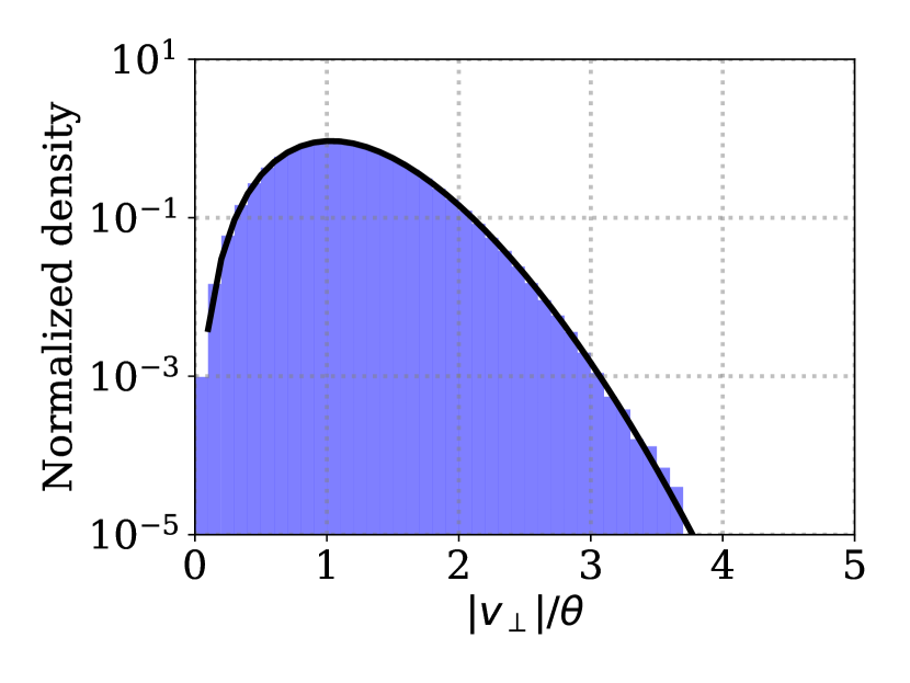
Figure 1: The distribution of $v_{\perp}$ of the subtracted Maxwellian ($\beta=0.5$). Monte Carlo results with $10^{6}$ particles (the blue histogram) and the theoretical curve (the black curve) are compared.

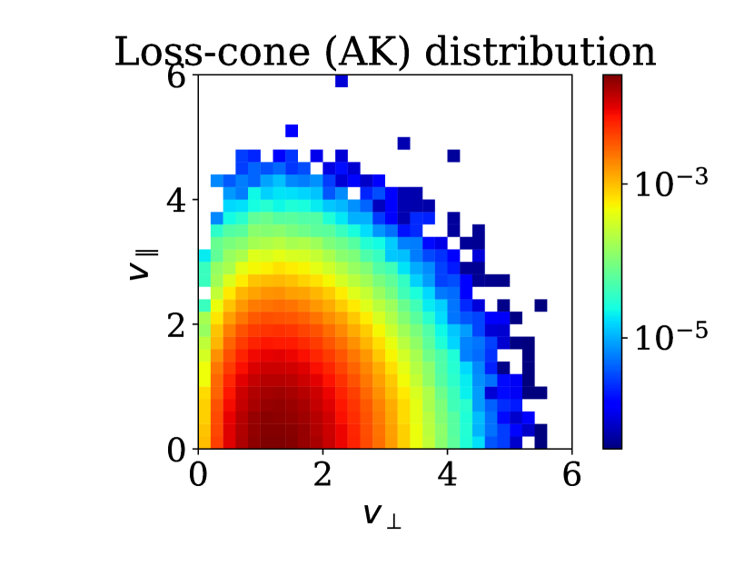
Figure 2: Monte Carlo sampling of the subtracted Maxwellian ($\beta=0.5$ and $\theta=1.5$) with $10^{6}$ particles. Phase-space density is presented in the $v_{\perp}$–$v_{\parallel}$ plane.

III Dory-type loss-cone distribution

Next we discuss another loss-cone model, proposed by Dory et al. (1965). This distribution is called Dory-type loss-cone distribution or Dory–Guest–Harris (DGH) distribution. It approximates a loss cone by using a power of the perpendicular velocity $\propto(v_{\perp}^{2})^{j}$. The loss-cone index $j$ is a non-negative number, $j\geq 0$.

$$f(v_{\parallel},\boldsymbol{v}_{\perp}) =\frac{N_{0}}{\pi^{3/2}\theta_{\parallel}\theta_{\perp}^{2}\Gamma(j+1)}\left(\frac{v_{\perp}}{\theta_{\perp}}\right)^{2j}\exp\left(-\frac{v^{2}_{\parallel}}{\theta_{\parallel}^{2}}-\frac{v_{\perp}^{2}}{\theta_{\perp}^{2}}\right)$$ (17)

$$P_{\parallel} =\frac{1}{2}N_{0}m\theta_{\parallel}^{2},~{}~{}~{}P_{\perp}=\frac{1}{2}N_{0}m\theta_{\perp}^{2}({1+j})$$ (18)

When the loss-cone index is $j=0$, the distribution is nearly a bi-Maxwellian. As the index increases, the loss cone becomes apparent. The subtracted Maxwellian with $\Delta=0$ and $\beta=1$ is identical to the Dory-type distribution with $j=1$. We similarly split the distribution into the parallel and perpendicular parts:

$$f(v_{\parallel},\boldsymbol{v}_{\perp}) =\frac{N_{0}}{\pi^{1/2}\theta_{\parallel}}\exp\left(-\frac{v^{2}_{\parallel}}{\theta_{\parallel}^{2}}\right)$$

$$~{}~{}~{}\times\frac{1}{\pi\theta_{\perp}^{2}\Gamma(j+1)}\left(\frac{v_{\perp}}{\theta_{\perp}}\right)^{2j}\exp\left(-\frac{v_{\perp}^{2}}{\theta_{\perp}^{2}}\right)$$ (19)

Again, we focus on the perpendicular part. Considering $v_{\perp 1}\equiv v_{\perp}\cos\varphi$ and $v_{\perp 2}\equiv v_{\perp}\sin\varphi$ in the cylindrical coordinates $(v_{\perp},\varphi,v_{\parallel})$, we rewrite the perpendicular part as

$$f_{V_{\perp}}(v_{\perp}) =\frac{2\pi v_{\perp}}{\pi\theta_{\perp}^{2}\Gamma(j+1)}\left(\frac{v_{\perp}^{2}}{\theta_{\perp}^{2}}\right)^{j}\exp\left(-\frac{v_{\perp}^{2}}{\theta_{\perp}^{2}}\right)$$ (20)

By setting $x\equiv v_{\perp}^{2}/\theta_{\perp}^{2}$, we find a gamma distribution with a shape parameter $j+1$.

$$f_{X}(x) =\frac{x^{j}e^{-x}}{\Gamma(j+1)}={\rm Ga}(x;j+1,1)$$ (21)

There are several algorithms to generate a gamma distribution. We recommend the readers to consult textbooks on random variates(Devroye, 1986; Yotsuji, 2010; Kroese et al., 2011) for detail, but we quickly outline the gamma-distribution generators here. Let us consider the gamma distribution with shape $k$ and scale $\lambda$, i.e. $\sim{\rm Ga}(k,\lambda)$. When $k$ is a integer, a gamma variate $x$ can be drawn by using multiple uniform random variates $Y_{i}\sim U(0,1)$ ($i=1,2,\dots,k$) in the following way,

$$x\leftarrow\lambda\sum_{i=1}^{k}\left(-\log Y_{i}\right)=-\lambda\log\left(\prod_{i=1}^{k}Y_{i}\right)$$ (22)

When $k$ is a half integer ($1/2,3/2,\cdots$), in addition to uniform variates $Y_{i}\sim U(0,1)$ ($i=1,2,\dots k-1/2$), we use one normal variate $n_{1}\sim\mathcal{N}(0,1)$,

$$x\leftarrow-\lambda\log\left(\prod_{i=1}^{k-1/2}Y_{i}\right)+\frac{\lambda}{2}n_{1}^{2}.$$ (23)

When $k>1$ is non-integer, Marsaglia & Tsang (2000)’s method is useful, as detailed by many textbooks. One can also use it for integer and non-integer cases, because it is known to be faster.

In the case of Eq. (21), we can generate a gamma variate $x\sim{\rm Ga}(j+1,1)$ by using Eq. (22). Then we similarly obtain $v_{\perp 1}$ and $v_{\perp 2}$. The procedure is outlined in Algorithm 3 in Table 2. The gamma generator for integer $j$ is written in the form of comments, in case we employ other algorithms for non-integer $j$. When $j=0$, the perpendicular part recovers the Box–Muller (1958) method to generate a Maxwellian.

We have numerically generated the Dory-type distribution of $10^{6}$ particles, according to Equation (17) with $j=2$. Fig. 3 shows the phase-space density in the $v_{\perp}$–$v_{\parallel}$ plane, in the same format as Fig. 2. To emphasize the internal structure, $\theta$ is set to $1.5$. There is a vertical hole with a steep density gradient along the $v_{\parallel}$ axis.

Table 2: Algorithm for the Dory-type loss-cone distribution

Algorithm 3
generate $X\sim{\rm Ga}(j+1,1)$
// generate $Y_{1},\cdots,Y_{j+1}\sim U(0,1)$
// $X\leftarrow-\log\big{(}\prod_{k=1}^{j+1}Y_{k}\big{)}$
generate $U\sim U(0,1)$
generate $N\sim\mathcal{N}(0,1)$
$v_{\perp 1}\leftarrow\theta_{\perp}\sqrt{X}\cos(2\pi U)$
$v_{\perp 2}\leftarrow\theta_{\perp}\sqrt{X}\sin(2\pi U)$
$v_{\parallel}~{}\leftarrow\theta_{\parallel}\sqrt{1/2}~{}N$
return $v_{\perp 1},v_{\perp 2},v_{\parallel}$

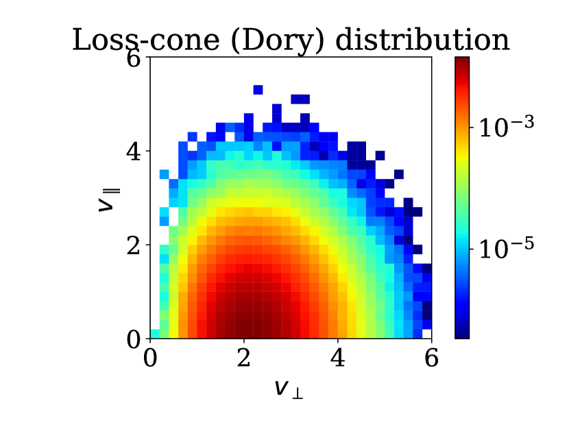
Figure 3: Monte Carlo sampling of the Dory-type loss-cone distribution ($\theta=1.5$ and $j=2$) with $10^{6}$ particles. Phase-space density is presented in the $v_{\perp}$–$v_{\parallel}$ plane.

IV Kappa loss-cone distribution

The kappa distribution(Vasyliunas, 1968; Olbert, 1968) extends the Maxwell distribution with a power-law tail in the high-energy part, and it has drawn huge attention in space physics.(Livadiotis, 2017) Recognizing the importance of the kappa distribution, Summers and Thorne (1991) have proposed a hybrid distribution of the kappa distribution and the Dory-type loss-cone distribution. It was sometimes called the (generalized) Lorentzian loss-cone distribution, while it is popularly referred to as the kappa loss-cone (KLC) distribution. In this paper, we occasionally call it the Summers-type KLC distribution to distinguish it from another variant in Section V.3. Its mathematical form is given by Summers and Thorne (1991, 1995):

$$f(\boldsymbol{v}) =\frac{N_{0}}{\pi^{3/2}\theta_{\parallel}\theta_{\perp}^{2}\kappa^{j+3/2}}\frac{\Gamma(\kappa+j+1)}{\Gamma(j+1)\Gamma(\kappa-1/2)}$$

$$~{}~{}~{}\times\left(\frac{v_{\perp}}{\theta_{\perp}}\right)^{2j}\Big{(}1+\frac{{v_{\parallel}}^{2}}{\kappa\theta_{\parallel}^{2}}+\frac{{v_{\perp}}^{2}}{\kappa\theta_{\perp}^{2}}\Big{)}^{-(\kappa+j+1)}$$ (24)

$$P_{\parallel} =\frac{\kappa}{2\kappa-3}N_{0}m\theta_{\parallel}^{2},~{}~{}~{}P_{\perp}=\frac{\kappa}{2\kappa-3}N_{0}m\theta_{\perp}^{2}(1+j)$$ (25)

Here, $\kappa$ ($>3/2$) is the kappa index and $j$ ($\geq 0$) is the loss-cone index. When $j=0$, the distribution recovers a standard (bi-)kappa distribution. When $j>0$, it develops a loss-cone.

The KLC distribution has nice mathematical properties. For example, in the isotropic case of $\theta_{\parallel}=\theta_{\perp}=\theta$, Eq. (IV) yields

$$f(\boldsymbol{v}) \propto\Big{(}1+\frac{{v}^{2}}{\kappa\theta^{2}}\Big{)}^{-(\kappa+1)}\left(\dfrac{\frac{v_{\perp}^{2}}{\kappa\theta^{2}}}{1+\frac{{v}^{2}}{\kappa\theta^{2}}}\right)^{j}$$

$$~{}~{}~{}\approx\Big{(}{\rm~{}\cdots~{}}\Big{)}^{-(\kappa+1)}\Big{(}\sin\alpha\Big{)}^{2j}$$ (26)

Along with a power-law tail with an index of $\kappa+1$, one can see that the loss-cone is approximated by the pitch angle $\alpha$ in the $v^{2}\gg\kappa\theta^{2}$ range, as was done in an earlier work.(Kennel, 1966)

Table 3: Algorithm for the Summers-type kappa loss-cone (KLC) distribution

Algorithm 4
generate $N\sim\mathcal{N}(0,1)$
generate $Y\sim{\rm Ga}(\kappa-1/2,2)$
generate $X\sim{\rm Ga}(j+1,2)$
generate $U\sim U(0,1)$
$v_{\perp 1}\leftarrow\theta_{\perp}\sqrt{\kappa X}\cos(2\pi U)/\sqrt{Y}$
$v_{\perp 2}\leftarrow\theta_{\perp}\sqrt{\kappa X}\sin(2\pi U)/\sqrt{Y}$
$v_{\parallel}~{}\leftarrow\theta_{\parallel}\sqrt{\kappa}N/\sqrt{Y}$
return $v_{\perp 1},v_{\perp 2},v_{\parallel}$

A numerical procedure for the Dory-type distribution was discussed in Section III. Procedures for the kappa distribution are also known.(Abdul & Mace, 2015; Zenitani & Nakano, 2022) For detail, the readers may wish to consult Section III in Zenitani & Nakano (2022) (Hereafter referred to as ZN22). Combining the procedures for the Dory distribution (Table 2) and for the kappa distribution (Table I in ZN22), we propose a novel procedure for the KLC distribution in Table 3. This algorithm uses two gamma-distributed variates. Their shape parameters can be an integer, a half-integer, and non-integer. In any case, we can obtain the random variates by using gamma generators in Section III. Below, we gives a formal proof that the new procedure generates the KLC distribution according to Eq. (IV).

We consider four independent random variates $X$, $N$, $Y$, and $U$. The first variate $X$ follows a gamma distribution with the shape parameter $j+1$ and the scale parameter 2, $X\sim{\rm Ga}(j+1,2)$. The second follows a normal distribution, $N\sim\mathcal{N}(0,1)$. The third follows a chi-squared distribution with $2\kappa-1$ degrees of freedom. This chi-squared distribution is equivalent to the gamma distribution of $Y\sim{\rm Ga}(\kappa-1/2,2)$. The last variate follows the uniform distribution, $U\sim U(0,1)$. Using the four variates, we define the following four variables.

$$V_{\perp 1} =\theta_{\perp}\sqrt{\kappa X}\cos(2\pi U)/\sqrt{Y}$$ (27)

$$V_{\perp 2} =\theta_{\perp}\sqrt{\kappa X}\sin(2\pi U)/\sqrt{Y}$$ (28)

$$V_{\parallel} =\theta_{\parallel}\sqrt{\kappa}N/\sqrt{Y}$$ (29)

$$Z =X+N^{2}+Y$$ (30)

We immediately obtain

$$X =\frac{V_{\perp}^{2}}{\kappa\theta_{\perp}^{2}}Y=\frac{V_{\perp}^{2}}{\kappa\theta_{\perp}^{2}}Z\left(1+\frac{V_{\parallel}^{2}}{\kappa\theta_{\parallel}^{2}}+\frac{V_{\perp}^{2}}{\kappa\theta_{\perp}^{2}}\right)^{-1}$$ (31)

$$N =\frac{V_{\parallel}}{\sqrt{\kappa}\theta_{\parallel}}\sqrt{Y}=\frac{V_{\parallel}}{\sqrt{\kappa}\theta_{\parallel}}\sqrt{Z}\left(1+\frac{V_{\parallel}^{2}}{\kappa\theta_{\parallel}^{2}}+\frac{V_{\perp}^{2}}{\kappa\theta_{\perp}^{2}}\right)^{-1/2}$$ (32)

$$Y =Z\left(1+\frac{V_{\parallel}^{2}}{\kappa\theta_{\parallel}^{2}}+\frac{V_{\perp}^{2}}{\kappa\theta_{\perp}^{2}}\right)^{-1}$$ (33)

With help from a chain rule, we calculate the following Jacobian

$$\left\|\frac{\partial(X,N,Y)}{\partial(V_{\perp},V_{\parallel},Z)}\right\| =\left\|\frac{\partial(X,N,Y)}{\partial(V_{\perp},V_{\parallel},Y)}\right\|\cdot\left\|\frac{\partial(V_{\perp},V_{\parallel},Y)}{\partial(V_{\perp},V_{\parallel},Z)}\right\|$$

$$=\frac{2V_{\perp}Y^{3/2}}{\kappa^{3/2}\theta_{\parallel}\theta_{\perp}^{2}}\cdot\left|\frac{\partial Y}{\partial Z}\right|$$

$$=\frac{2V_{\perp}Z^{3/2}}{\kappa^{3/2}\theta_{\parallel}\theta_{\perp}^{2}}\left(1+\frac{V_{\parallel}^{2}}{\kappa\theta_{\parallel}^{2}}+\frac{V_{\perp}^{2}}{\kappa\theta_{\perp}^{2}}\right)^{-5/2}$$ (34)

We consider the joint probability distribution function of $X$, $N$, and $Y$. Since the three variates are independent, the function is a product of the gamma distribution of $x$, the normal distribution of $n$, and the gamma distribution of $y$,

$$f_{X,N,Y}(x,n,y)=\left(\frac{x^{j}e^{-x/2}}{\Gamma(j+1)2^{j+1}}\right)\times\left(\frac{1}{\sqrt{2\pi}}e^{-n^{2}/2}\right)\times\left(\frac{y^{\kappa-3/2}e^{-y/2}}{\Gamma(\kappa-1/2)2^{\kappa-1/2}}\right)$$ (35)

Using Eqs. (31)–(IV), we translate Eq. (35) into

$$f_{V_{\perp},V_{\parallel},Z}(v_{\perp},v_{\parallel},z) =\frac{z^{j+\kappa-3/2}e^{-z/2}}{\sqrt{\pi}\Gamma(j+1)\Gamma(\kappa-1/2)2^{j+\kappa+1}}\left(\frac{v_{\perp}^{2}}{\kappa\theta_{\perp}^{2}}\right)^{j}\left(1+\frac{v_{\parallel}^{2}}{\kappa\theta_{\parallel}^{2}}+\frac{v_{\perp}^{2}}{\kappa\theta_{\perp}^{2}}\right)^{-j-\kappa+3/2}\left\|\frac{\partial(X,N,Y)}{\partial(V_{\perp},V_{\parallel},Z)}\right\|$$

$$=\frac{2\pi v_{\perp}}{\kappa^{3/2}\theta_{\parallel}\theta_{\perp}^{2}}\frac{z^{j+\kappa}e^{-z/2}}{\pi^{3/2}\Gamma(j+1)\Gamma(\kappa-1/2)2^{j+\kappa+1}}\left(\frac{v_{\perp}^{2}}{\kappa\theta_{\perp}^{2}}\right)^{j}\left(1+\frac{v_{\parallel}^{2}}{\kappa\theta_{\parallel}^{2}}+\frac{v_{\perp}^{2}}{\kappa\theta_{\perp}^{2}}\right)^{-(j+\kappa+1)}$$

$$=\left(\frac{z^{j+\kappa}e^{-z/2}}{2^{j+\kappa+1}\Gamma(j+\kappa+1)}\right)$$

$$~{}~{}~{}\times\left\{\frac{1}{{\pi}^{3/2}\theta_{\parallel}\theta_{\perp}^{2}\kappa^{j+3/2}}\frac{\Gamma(j+\kappa+1)}{\Gamma(j+1)\Gamma(\kappa-1/2)}\left(\frac{v_{\perp}}{\theta_{\perp}}\right)^{2j}\left(1+\frac{v_{\parallel}^{2}}{\kappa\theta_{\parallel}^{2}}+\frac{v_{\perp}^{2}}{\kappa\theta_{\perp}^{2}}\right)^{-(j+\kappa+1)}2\pi v_{\perp}\right\}$$ (36)

This tells us that the variable $Z$ follows the gamma distribution with shape $j+\kappa+1$ and scale $2$, $Z\sim{\rm Ga}(j+\kappa+1,2)$, and the other variables $V_{\perp}$ and $V_{\parallel}$ are distributed by the KLC distribution (Eq. (IV)), with trivial translation of $V_{\perp}\rightarrow(V_{\perp 1},V_{\perp 2})$. Eq. (36) also indicates that the two distributions are independent.

Mathematically, it is reasonable that $Z$ follows the gamma distribution. The square of the normal distribution $N$ provides a chi-squared distribution with one degree of freedom, which is equivalent to the gamma distribution ${\rm Ga}(1/2,2)$. This means that $Z$ is a sum of the three gamma distributions with the same scale parameter (Eq. (30)). In such a case, it is known that their sum follows a gamma distribution with the summed shape parameter: $Z\sim{\rm Ga}\left((\kappa-\frac{1}{2})+\frac{1}{2}+(j+1),2\right)$, in agreement with Eq. (36).

Figure 4: Monte Carlo sampling of the KLC distribution ($\theta=1.0$, $j=2$, and $\kappa=3.5$) with $10^{6}$ particles. Phase-space density is shown in $v_{\perp}$–$v_{\parallel}$.

Using Algorithm 4 in Table 3, we have numerically generated the KLC distribution with $10^{6}$ particles. The parameters are set to $\theta_{\perp}=\theta_{\parallel}=1.0$, $j=2$ and $\kappa=3.5$. Figure 4 shows the phase-space density in the $v_{\perp}$–$v_{\parallel}$ space in the same format. There is a vertical hole near the $v_{\parallel}$ axis, and plasmas are widely spread over the velocity space. In the horizontal direction (at $v_{\parallel}=0$), the phase-space density decays like $\propto v_{\perp}^{-2(\kappa+1)}=v_{\perp}^{-9.0}$. As $v_{\perp}$ increases, it drops slower than in the other loss-cone distributions ($\propto\exp[-(v_{\perp}^{2}/\theta_{\perp}^{2})]$). The numerical results are in excellent agreement with the analytic solution, as will be shown later.

V Pitch-angle-type loss-cone distributions

V.1 Acceptance-rejection method

In the Dory and KLC distributions, the loss cone is modeled by a power of the perpendicular velocity, $\propto(v_{\perp})^{2j}$. Consequently, the “loss cone” often looks like a vertical hole, as evident in Figures 3 and 4. In this section, we consider another loss-cone model, whose phase-space density is modeled by the pitch angle $\alpha$, i.e.,

$$\propto(\sin\alpha)^{2j}=\left(\frac{v_{\perp}}{v}\right)^{2j}$$ (37)

as considered in an earlier work.(Kennel, 1966) We call it the pitch-angle-type (PA-type) loss-cone distribution.

The easiest way to generate a PA-type distribution is to generate an isotropic distribution, which we call the base distribution, and then to employ the acceptance-rejection method. Using a uniform variate $U\sim U(0,1)$, we accept the particle when the following condition is met,

$$U<\left(\frac{v_{\perp}}{v}\right)^{2j}$$ (38)

If this condition is not met, we reject the particle, and then we regenerate the random variate. Then we can straightforwardly obtain the loss-cone distribution, based on Eq. (37).

Let us evaluate the acceptance efficiency of this rejection method. We consider the spherical coordinates $(v,\alpha,\varphi)$ as illustrated in Fig. 5. Since the base distribution $f_{0}$ is spherically symmetric, it satisfies

$$f_{0}(\boldsymbol{v})~{}d^{3}v=f_{0}(v,\alpha,\varphi)~{}v^{2}\sin\alpha~{}dvd\alpha d\varphi=f_{0}(v)~{}v^{2}\sin\alpha~{}dvd\alpha d\varphi$$ (39)

We further impose an additional weight of Eq. (37), i.e., $f(v)\propto f_{0}(v)~{}(\sin\alpha)^{2j}$. The total weight $W(j)$ is estimated by

$$W(j) \equiv\dfrac{\iiint f_{0}(\boldsymbol{v})~{}(\sin\alpha)^{2j}d^{3}v}{\iiint f_{0}(\boldsymbol{v})~{}d^{3}v}=\dfrac{\int_{0}^{\infty}dv\int_{0}^{\pi}d\alpha\int_{0}^{2\pi}d\varphi~{}\Big{\{}f_{0}(v)~{}v^{2}(\sin\alpha)^{2j+1}\Big{\}}}{\int_{0}^{\infty}dv\int_{0}^{\pi}d\alpha\int_{0}^{2\pi}d\varphi~{}\Big{\{}f_{0}(v)~{}v^{2}(\sin\alpha)\Big{\}}}$$

$$=\dfrac{4\pi\Big{(}\int_{0}^{\infty}v^{2}f_{0}(v)~{}dv\Big{)}\Big{(}\int_{0}^{\pi/2}\left(\sin\alpha\right)^{2j+1}d\alpha\Big{)}}{4\pi\int_{0}^{\infty}v^{2}f_{0}(v)~{}dv}=\int_{0}^{\pi/2}\left(\sin\alpha\right)^{2j+1}d\alpha$$ (40)

By setting $x\equiv\cos^{2}\alpha$, we obtain

$$W(j) =\frac{1}{2}\int_{0}^{1}(1-x)^{j}x^{-1/2}dx=\dfrac{B(1/2,j+1)}{2}\int_{0}^{1}{\rm Beta}\left(x;\frac{1}{2},j+1\right)dx$$

$$=\dfrac{\sqrt{\pi}}{2}\cdot\dfrac{\Gamma(j+1)}{\Gamma(j+3/2)}$$ (41)

where $B(\alpha,\beta)$ is the beta function and ${\rm Beta}(x;\alpha,\beta)$ is the probability density function of the beta distribution. Since Eq. (41) is normalized, it immediately gives the total acceptance efficiency of the acceptance-rejection method. As shown in Fig. 6, Eq. (41) monotonically decreases from $1$ at $j=0$ to $0$ at $j\rightarrow\infty$. The efficiency decays slowly, and so the acceptance-rejection method would be useful for small $j$.

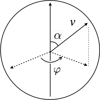
Figure 5: Our spherical coordinates: velocity $v$ ($|\boldsymbol{v}|)$, pitch angle $\alpha$, and azimuthal angle $\varphi$.

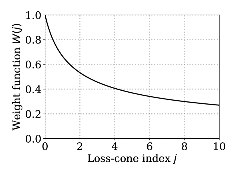
Figure 6: The weight function $W$ as a function of the loss-cone index $j$ (Eq. (41))

V.2 Loss-cone transform methods

Recognizing that $x=\cos^{2}\alpha$ is distributed under the beta distribution in Eq. (41), we propose an algorithm to transform an isotropic distribution into a PA-type loss-cone distribution. We first obtain a radial profile of the base distribution, $f_{0}(v)4\pi v^{2}$. Then we scatter the direction of particle velocity, by using a beta-distributed variate. This method does not reject any particles.

A random variate following the beta distribution can be generated from two gamma-distributed variates,(Devroye, 1986; Yotsuji, 2010; Kroese et al., 2011)

$$\dfrac{X_{\rm Ga(1/2,\lambda)}}{X_{\rm Ga(1/2,\lambda)}+X_{\rm Ga(j+1,\lambda)}}\sim{\rm Beta}(x;1/2,j+1)$$ (42)

where $X_{\rm Ga(k,\lambda)}$ is a random variate following the gamma distribution with shape $k$ and scale $\lambda$. This $\lambda$ is an arbitrary number, and we set $\lambda=2$ for convenience. Mathematically, ${\rm Ga(1/2,2)}$ is equivalent to the chi-squared distribution with 1 degree of freedom, which can be obtained from a square of the normal distribution. Using a normal variate $N\sim\mathcal{N}(0,1)$ and considering $0\leq\alpha\leq\pi$, we can generate the distribution of the cosine of the pitch angle

$$\cos\alpha\sim\dfrac{N}{\sqrt{N^{2}+X_{\rm Ga(j+1,2)}}},$$ (43)

For given $|v|$, we obtain $v_{\parallel}=|v|\cos\alpha$ and $v_{\perp}=|v|\sin\alpha=|v|(1-\cos^{2}\alpha)^{1/2}$, and then we can further obtain $v_{\perp 1}$ and $v_{\perp 2}$ by randomly setting the azimuthal angle. The numerical procedure is summarized in Algorithm 5.1 in Table 4. We call it the loss-cone transform method. Applications to the Maxwell and kappa distribution will be presented in Section V.3.

Table 4: Loss-cone transform algorithms

Algorithm 5.1: loss-cone transform
$v\mapsto{v}_{\perp 1},{v}_{\perp 2},{v}_{\parallel}$
generate $N\sim\mathcal{N}(0,1)$
generate $X\sim{\rm Ga}(j+1,2)$
generate $U\sim U(0,1)$
${v}_{\perp 1}\leftarrow v~{}\sqrt{\dfrac{X}{N^{2}+X}}\cos(2\pi U)$
${v}_{\perp 2}\leftarrow v~{}\sqrt{\dfrac{X}{N^{2}+X}}\sin(2\pi U)$
${v}_{\parallel}~{}\leftarrow v~{}\dfrac{N}{\sqrt{N^{2}+X}}$
return ${v}_{\perp 1},{v}_{\perp 2},{v}_{\parallel}$

Algorithm 5.2: latitude transform
${v}_{\perp 1},{v}_{\perp 2},{v}_{\parallel}\mapsto\bar{v}_{\perp 1},\bar{v}_{\perp 2},\bar{v}_{\parallel}$
$v^{2}_{\perp}\leftarrow v_{\perp 1}^{2}+v_{\perp 2}^{2}$
$v\leftarrow\sqrt{v_{\perp}^{2}+v_{\parallel}^{2}}$
$\bar{v}_{\parallel}\leftarrow v~{}C^{-1}\left({v_{\parallel}}/{v};j\right)$
$\bar{v}_{\perp 1}\leftarrow\sqrt{v^{2}-\bar{v}_{\parallel}^{2}}~{}\dfrac{v_{\perp 1}}{v_{\perp}}$
$\bar{v}_{\perp 2}\leftarrow\sqrt{v^{2}-\bar{v}_{\parallel}^{2}}~{}\dfrac{v_{\perp 2}}{v_{\perp}}$
return $\bar{v}_{\perp 1},\bar{v}_{\perp 2},\bar{v}_{\parallel}$

In the loss-cone transform algorithm, particle velocities are randomly scattered into all the directions. Here we propose another transform algorithm that only adjusts the pitch angle but preserves the azimuthal angle. We assume $j$ to be an integer in this subsection. We consider a cumulative distribution function (CDF) of $x$. The CDF of the beta distribution is given by the regularized incomplete beta function, $I_{x}$.

$$C(x;j) =I_{x}(1/2,j+1)=\frac{{\rm Beta}(x;1/2,j+1)}{B(1/2,j+1)}$$

$$=\frac{2\sqrt{x}~{}{}_{2}F_{1}(1/2,-j;3/2;x)}{B(1/2,j+1)}$$ (44)

Here, we have used a relation in Abramowitz & Stegun (1972) and ${}_{2}F_{1}$ is the hypergeometric function. We further set the cosine to $u=\cos\alpha$. We temporarily limit our attention to $0\leq u\leq 1$, and then obtain a CDF

$$C(u;j)=\frac{2u~{}{}_{2}F_{1}(1/2,-j;3/2;u^{2})}{B(1/2,j+1)}$$ (45)

This gives

$$C(u;0) =u$$ (46)

$$C(u;1) =\frac{3}{2}u-\frac{1}{2}u^{3}$$ (47)

$$C(u;2) =\frac{15}{8}u-\frac{5}{4}u^{3}+\frac{3}{8}u^{5}$$ (48)

$$C(u;3) =\cdots$$ (49)

These are non-injective functions, but they are monotonic in $-1\leq u\leq 1$. Thus we can define their inverse functions, $C^{-1}(x;j)$ in this range. When we transform an isotropic distribution into a loss-cone distribution, we map the cosine latitude $u_{0}\mapsto u_{j}$ such that

$$C(u_{0};0) =u_{0}=C(u_{j};j).$$ (50)

Thus, we obtain $u_{j}=C^{-1}(u_{0};j)$ via the inverse function, which also works for the negative case of $-1\leq u<0$. After modifying the latitude, then we adjust $\sin\alpha$ accordingly. These procedures are summarized in Algorithm 5.2 in Table 4. We call this method the latitude transform method. The azimuthal angle in the velocity space is conserved. The inverse function can be calculated by interpolating and looking up a numerical table of the CDF.

Table 5: Algorithms for the PA-type distributions.

Algorithm 5.3: Loss-cone distribution
generate $N\sim\mathcal{N}(0,1)$
generate $X_{1}\sim{\rm Ga}(3/2,1)$
generate $X_{2}\sim{\rm Ga}(j+1,2)$
generate $U\sim U(0,1)$
$v_{\perp 1}\leftarrow\theta\sqrt{X_{1}}~{}\sqrt{\dfrac{X_{2}}{N^{2}+X_{2}}}\cos(2\pi U)$
$v_{\perp 2}\leftarrow\theta\sqrt{X_{1}}~{}\sqrt{\dfrac{X_{2}}{N^{2}+X_{2}}}\sin(2\pi U)$
$v_{\parallel}~{}\leftarrow\theta\sqrt{X_{1}}~{}\dfrac{N}{\sqrt{N^{2}+X_{2}}}$
return $v_{\perp 1},v_{\perp 2},v_{\parallel}$

Algorithm 5.4: KLC distribution
generate $N\sim\mathcal{N}(0,1)$
generate $Y\sim{\rm Ga}(\kappa-1/2,2)$
generate $X_{1}\sim{\rm Ga}(3/2,2)$
generate $X_{2}\sim{\rm Ga}(j+1,2)$
generate $U\sim U(0,1)$
$v_{\perp 1}\leftarrow\theta\sqrt{\dfrac{\kappa X_{1}}{Y}}\sqrt{\dfrac{X_{2}}{N^{2}+X_{2}}}\cos(2\pi U)$
$v_{\perp 2}\leftarrow\theta\sqrt{\dfrac{\kappa X_{1}}{Y}}\sqrt{\dfrac{X_{2}}{N^{2}+X_{2}}}\sin(2\pi U)$
$v_{\parallel}~{}\leftarrow\theta\sqrt{\dfrac{\kappa X_{1}}{Y}}\dfrac{N}{\sqrt{N^{2}+X_{2}}}$
return $v_{\perp 1},v_{\perp 2},v_{\parallel}$

V.3 Loss-cone and kappa loss-cone distributions

Here, we show practical applications of the loss-cone transform method. We first discuss the following PA-type loss-cone distribution. This one is based on the isotropic Maxwellian.

$$f(\boldsymbol{v}) =\frac{N_{0}}{\pi^{2}\theta^{3}}\frac{2\Gamma(j+3/2)}{\Gamma(j+1)}\Big{(}\frac{v_{\perp}}{v}\Big{)}^{2j}\exp\Big{(}-\frac{v^{2}}{\theta^{2}}\Big{)}$$ (51)

$$P_{\parallel} =\frac{3}{2}~{}\frac{1}{2j+3}N_{0}m\theta^{2},~{}~{}~{}P_{\perp}=\frac{3}{2}~{}\frac{j+1}{2j+3}N_{0}m\theta^{2}$$ (52)

Note that the normalization constant in Eq. (51) is rescaled by Eq. (41). It looks complicated, but it usually does not appear in algorithms. In Section II in ZN22, the authors discussed that $|v|$ in the Maxwellian follows the gamma distribution with shape $k=3/2$.

$$f(v) \propto 4\pi v^{2}\exp\Big{(}-\frac{v^{2}}{\theta^{2}}\Big{)}\sim{\rm Ga}(3/2,1)$$ (53)

Then $v$ is given by a gamma-distributed variate.

$$v=\theta\sqrt{X_{{\rm Ga}(3/2,1)}}$$ (54)

After generating $v$ using a gamma-distribution generator, we employ the loss-cone transform method in Section V.2 to obtain the PA-type loss-cone distribution. The entire procedure is summarized in Algorithm 5.3 in Table 5.

Finally, we similarly construct a procedure for the PA-type kappa loss-cone (KLC) distribution. This form is consistent with one in an earlier literature.(Xiao et al., 1998)

$$f(\boldsymbol{v}) =\frac{N_{0}}{\pi^{2}\theta^{3}\kappa^{3/2}}\frac{2\Gamma(j+3/2)\Gamma(\kappa+1)}{\Gamma(j+1)\Gamma(\kappa-1/2)}$$

$$~{}~{}~{}\times\Big{(}\frac{v_{\perp}}{v}\Big{)}^{2j}\Big{(}1+\frac{v^{2}}{\kappa\theta^{2}}\Big{)}^{-(\kappa+1)}$$ (55)

$$P_{\parallel} =\frac{3\kappa}{2\kappa-3}~{}\frac{1}{2j+3}N_{0}m\theta^{2},~{}P_{\perp}=\frac{3\kappa}{2\kappa-3}~{}\frac{j+1}{2j+3}N_{0}m\theta^{2}$$ (56)

In Section III in ZN22, the authors have shown that the $|v|$ distribution of the kappa distribution

$$f(v) ~{}\propto~{}4\pi v^{2}\Big{(}1+\frac{{v}^{2}}{\kappa\theta^{2}}\Big{)}^{-(\kappa+1)}$$ (57)

is obtained from two gamma-distributed variates.

$$v=\left(\kappa\theta^{2}\frac{X_{{\rm Ga}(3/2,2)}}{X_{{\rm Ga}(\kappa-1/2,2)}}\right)^{1/2}$$ (58)

Combining this with the loss-cone transform method, we generate the PA-type KLC distribution. The entire procedure is summarized in Algorithm 5.4 in Table 5.

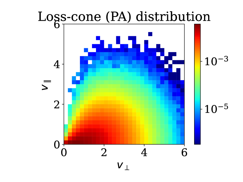
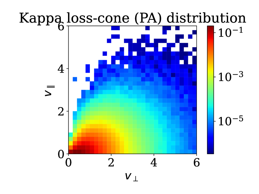
Figure 7: Monte Carlo sampling of the pitch angle (PA)-type loss-cone distribution ($\theta=2.0$ and $j=2.0$) with $10^{6}$ particles. Phase-space density is shown in $v_{\perp}$–$v_{\parallel}$.

Figure 8: Monte Carlo sampling of the pitch angle (PA)-type KLC distribution ($\theta=1.0$, $j=2.0$, and $\kappa=3.5$) with $10^{6}$ particles. Phase-space density is shown in $v_{\perp}$–$v_{\parallel}$.

Using $10^{6}$ particles, we have numerically generated the PA-type loss-cone distribution with $\theta=2$ and $j=2$ and the PA-type KLC distribution with $\theta=1.0$, $j=2$, and $\kappa=3.5$, respectively. Figs. 8 and 8 show their phase-space densities in $v_{\perp}$–$v_{\parallel}$ in the same format as other plots. The density cavities near the $v_{\parallel}$ axis look very different from those in the other distributions (Figs. 2, 3, and 4). It is cone-shaped in the PA-type distributions, while it looks like a vertical hole in the other distributions. It is clear that the PA-type distribution better approximates the loss-cone.

VI Numerical tests

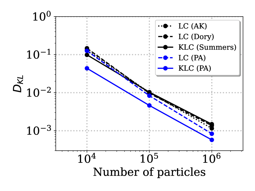
Figure 9: The Kullback–Leibler divergence of the numerical distributions from the analytical solutions (Eq. (60)).

To verify the numerical results for multidimensional velocity distribution functions, we evaluate the Kullback–Leibler (KL) divergence between the analytic solutions and our Monte Carlo results. The KL divergence between two probability distributions, $P$ and $Q$, are defined by

$$D_{\rm{KL}}(P\|Q)=\sum_{i}P(i)\log\frac{P(i)}{Q(i)}$$ (59)

This quantifies the deviation of $Q$ from the other distribution $P$, and approaches zero when the two distributions are similar. For the target probability distributions $Q(i)$, we use our Monte Carlo data in the 2-D mesh in the $v_{\perp}$–$v_{\parallel}$ space with $\Delta v=1/5$, which we have used for our 2-D plots (Figs. 2, 3, 4, 8, and 8). For the baseline probability distributions $P(i)$, we have numerically integrated the analytic solution by using the same mesh. In practice, we use a very small number $\epsilon=10^{-10}$ to avoid $\log 0$,

$$D_{\rm{KL}}(P\|Q)\equiv\sum_{i}(P(i)+\epsilon)\log\frac{P(i)+\epsilon}{Q(i)+\epsilon}$$ (60)

Fig. 9 shows $D_{\rm{KL}}$ for all the multidimensional velocity distributions, as a function of the particle numbers. The absolute value of the KL divergence is unimportant, because it is even affected by the seed of the random numbers. Here, it is important to see that the KL divergence approaches zero, as we increase the particle number. This tells us that the Monte Carlo algorithms successfully generate the velocity distributions.

VII Discussion and Summary

In this article, we have proposed a series of numerical procedures that generate loss-cone distributions in particle simulations. Since many previous authors may have used the acceptance-rejection method, we discuss key differences between the acceptance-rejection method and the proposed methods.

The acceptance-rejection method needs a good sampling distribution. Sometimes we combine multiple sampling distributions, for example, the uniform distribution near the maximum and the power-law distribution for the high-energy tail. In such a case, the program has multiple logical branches. Then, for each particle, the program has a rejection loop. Comparing the target distribution and the sampling distribution, we accept or reject the particle at some probability. Since the acceptance rate is less than 100%, we need to repeat the same procedure again and again, until accepted. Technically, the program requires several random variates and conditional statements (if-else statements) to switch the branches and to accept/reject the particle inside the loop. The number of iterations is not fixed.

Most of the proposed methods (in Sections II–IV, V.2, and V.3) generate the loss-cone distribution functions from uniform, normal, and gamma random variates. The key features, such as the vertical or cone-shaped density hole and the power-law tail of the KLC distributions, are reproduced by the combinations of the variates. As can be seen in Tables, the procedures are simple. The algorithms do not have logical branches or loops. They do not even contain a conditional statement. Since we do not need to repeat the procedure, the number of operations is fixed. There features are favorable for parallel computing on GPUs and SIMD processors. We can take full advantage of these processors, when we execute the same instruction for multiple data.

The computational cost often depends on the total number of random variates. The proposed methods require a small number of random variates. For example, for the subtracted Maxwellian, Algorithm 2 requires two variates per particle (Eq. (10)) to obtain the $v_{\perp}$ (or $x$) distribution. In contrast, the acceptance-rejection method typically need two or more variates — one or more to distribute $v_{\perp}$ (or $x$) and another one to accept or reject the particle. As the acceptance rate is below 100%, some more will be necessary. Therefore, Algorithm 2 appears to be the best choice for the subtracted Maxwellian. For other distributions, our methods often rely on the gamma random generator. The costs depends on one’s choices of the gamma generators. The two generators in Section III (Eqs. (22) and (23)) use multiple random variates, in particular when the shape parameter $k$ is large. In case they are slow, one may try the Marsaglia & Tsang (2000) method instead, which is relatively insensitive to $k$.

In the Dory-type and PA-type loss-cone distributions and in the KLC distributions, the loss-cone index $j$ controls the opening angle of the loss-cone. In the KLC distributions, the kappa index $\kappa$ controls the spectral index of the power-law tail. We emphasize that these indices are not limited to integers. They are arbitrary in the range $j\geq 0$ and $\kappa>3/2$. For example, one can set $j=1/2$ or even less to obtain a narrow loss-cone. In practice, we can just use the gamma generators for half- or non-integer shape parameters, as outlined in Section III (Appendix A in ZN22 also provides a quick summary).

To construct the PA-type loss-cone distributions, we started from isotropic base distributions. We can also consider anisotropic variants of the PA-type distributions. We simply need to replace

$$\frac{1}{\theta^{3}}\rightarrow\frac{1}{\theta_{\parallel}\theta_{\perp}^{2}},~{}~{}\frac{v^{2}}{\theta^{2}}\rightarrow\frac{v_{\parallel}^{2}}{\theta_{\parallel}^{2}}+\frac{v_{\perp}^{2}}{\theta_{\perp}^{2}}$$ (61)

$$\Big{(}\frac{v_{\perp}}{v}\Big{)}^{2j}\rightarrow\left(\dfrac{{v_{\perp}^{2}}/{\theta_{\perp}^{2}}}{{v_{\parallel}^{2}}/{\theta_{\parallel}^{2}}+{v_{\perp}^{2}}/{\theta_{\perp}^{2}}}\right)^{j}$$ (62)

in Eqs. (51) or (55), and then $\theta\rightarrow\theta_{\perp}$ for $v_{\perp 1},v_{\perp 2}$ and $\theta\rightarrow\theta_{\parallel}$ for $v_{\parallel}$ in algorithms in Table 5. Meanwhile, the fractional equation in parentheses in Eq. (62) no longer mean the sine square of the pitch angle.

The loss-cone transform methods are also applicable to relativistic velocity distributions. In fact, the authors have presented numerical procedures to load a relativistic Maxwell distribution and a relativistic kappa distribution in ZN22. In these cases, we generate the radial profile of the relativistic four-velocity $\boldsymbol{u}=\gamma\boldsymbol{v}=[1-(v/c)^{2}]^{-1/2}\boldsymbol{v}$. Thus, one can straightforwardly combine these algorithms and the loss-corn transform methods, to generate relativistic loss-cone and relativistic KLC distributions.(Xiao et al., 1998)

In summary, we have presented Monte Carlo algorithms to generate loss-cone distributions, the subtracted Maxwellian (AK-type loss-cone distribution), the Dory-type loss-cone distribution, and the Summers-type KLC distributions. We have further presented another family of distributions, the PA-type loss-cone distributions. We have proposed the loss-cone transform methods, one of which are applied to the PA-type loss-cone and KLC distributions. Numerical recipes for all these distributions and the transform methods are provided in Tables. With some help from gamma-distribution generators, these algorithms can be easily implemented in one’s own code.

Author Declarations

Conflict of Interest

The authors have no conflicts to disclose.

Author Contributions

Seiji Zenitani: Conceptualization (lead), Formal analysis (equal), Investigation (lead), Methodology (lead), Visualization (lead), Writing – original draft (lead), Writing – review & editing (equal), Shin’ya Nakano: Formal analysis (equal), Methodology (supporting), Writing – review & editing (equal)

Data Availability Statement

The Jupyter notebook to generate the figures is available at arXiv:2309.06879 as an Ancillary file.

References

- Abdul & Mace (2015) R. F. Abdul and R. L. Mace, “One-dimensional particle-in-cell simulations of electrostatic Bernstein waves in plasmas with kappa velocity distributions,” Phys. Plasmas 22, 102107, doi:10.1063/1.4933005 (2015).
- Abramowitz & Stegun (1972) M. Abramowitz and I. A. Stegun, Handbook of Mathematical Functions with Formulas, Graphs, and Mathematical Tables, Dover, New York (1972), (Sections 6.6 and 26.5).
- Aschwanden (2006) M. J. Aschwanden, Physics of the Solar Corona: An Introduction with Problems and Solutions (2nd Edition), Springer (2006).
- Ashour-Abdalla & Kennel (1978) M. Ashour-Abdalla and C. F. Kennel, “Nonconvective and convective electron cyclotron harmonic instabilities,” J. Geophys. Res. 83, 1531, doi:10.1029/JA083iA04p01531 (1978).
- Benacek & Karlicky (2018) J. Benáček and M. Karlický, “Double plasma resonance instability as a source of solar zebra emission,” Astron. & Astrophys. 611, A60 (2018).
- Box–Muller (1958) G. E. P. Box and M. E. Muller, “A note on the generation of random normal deviates,” Ann. Math. Stat. 29, 610 (1958).
- Devroye (1986) L. Devroye, Non-Uniform Random Variate Generation, Springer-Verlag (1986), Chap. 9, p. 404.
- Dory et al. (1965) R. A. Dory, G. E. Guest, and E. G. Harris, “Unstable Electrostatic Plasma Waves Propagating Perpendicular to a Magnetic Field,” Phys. Rev. Lett. 14, 131, doi:10.1103/PhysRevLett.14.131 (1965).
- Friedel et al. (2002) R. H. W. Friedel, G. D. Reeves, and T. Obara, “Relativistic electron dynamics in the inner magnetosphere - a review,” J. Atmos. Solar Terr. Phys. 64, 265–282 (2002).
- Golkowski et al. (2019) M. Golkowski, V. Harid and P. Hosseini, “Review of Controlled Excitation of Nonlinear Wave-Particle Interactions in the Magnetosphere,” Front. Astron. Space Sci. 6, 2, doi:10.3389/fspas.2019.00002 (2019).
- Hikishima et al. (2009) M. Hikishima, S. Yagitani, Y. Omura, and I. Nagano, “Full particle simulation of whistler-mode rising chorus emissions in the magnetosphere,” J. Geophys. Res. 114, A01203 (2009).
- Katoh & Omura (2006) Y. Katoh and Y. Omura, “A study of generation mechanism of VLF triggered emission by self-consistent particle code,” J. Geophys. Res. 111, A12207, doi:10.1029/2006JA011704 (2006).
- Kennel (1966) C. F. Kennel, “Low-Frequency Whistler Mode,” Phys. Fluids 9, 2190 (1966).
- Kroese et al. (2011) D. P. Kroese, T. Taimre, and Z. I. Botev, Handbook of Monte Carlo methods, John Wiley & Sons. (2011).
- Livadiotis (2017) G. Livadiotis (ed.), Kappa Distributions: Theory and Applications in Plasmas, Elsevier, Amsterdam (2017).
- Marsaglia & Tsang (2000) G. Marsaglia and W. W. Tsang, “A Simple Method for Generating Gamma Variables,” ACM Transactions on Mathematical Software 26, 363 (2000).
- Melrose & Dulk (1982) D. B. Melrose and G. A. Dulk, “Electron-cyclotron masers as the source of certain solar and stellar radio bursts,” Astrophys. J. 259, 844 (1982).
- Ni et al. (2020) S. Ni, Y. Chen, C. Li, Z. Zhang, H. Ning, X. Kong, B. Wang, and M. Hosseinpour, “Plasma Emission Induced by Electron Cyclotron Maser Instability in Solar Plasmas with a Large Ratio of Plasma Frequency to Gyrofrequency,” Astrophys. J. 891, L25 (2020).
- Ning et al. (2021) H. Ning, Y. Chen, S. Ni, C. Li, Z. Zhang, X. Kong, and M. Yousefzadeh, “Harmonic Maser Emissions from Electrons with Loss-cone Distribution in Solar Active Regions,” Astrophys. J. 920, L40 (2021).
- Olbert (1968) S. Olbert, “Summary of Experimental Results from M.I.T. Detector on IMP-1,” in Physics of the Magnetosphere, eds. R. L. Carovillano, J. F. McClay, & H. R. Radoski (Astrophysics and Space Science Library, Vol. 10; Dordrecht: Reidel), 641 (1968).
- Pritchett (1984) P. L. Pritchett, “Electron-cyclotron maser radiation from a relativistic loss-cone distribution,” Phys. Fluids 27, 2393, doi:10.1063/1.864542 (1984).
- Shoji & Omura (2011) M. Shoji and Y. Omura, “Simulation of electromagnetic ion cyclotron triggered emissions in the Earth’s inner magnetosphere,” J. Geophys. Res. 116, A05212 (2011).
- Summers and Thorne (1991) D. Summers and R. M. Thorne, “The modified plasma dispersion function,” Phys. Fluids B 3, 1835, doi:10.1063/1.859653 (1991).
- Summers and Thorne (1995) D. Summers and R. M. Thorne, “lasma microinstabilities driven by loss-cone distributions,” J. Plasma Physics 53 293-315 (1995).
- Summers & Tang (2021) D. Summers and R. Tang, J. Geophys. Res. 126, e2020JA028276. doi:10.1029/2020JA028276 (2021).
- Tao (2014) X. Tao, “A numerical study of chorus generation and the related variation of wave intensity using the DAWN code,” J. Geophys. Res. 119, 3362, doi:10.1002/2014JA019820 (2014).
- Thorne (2010) R. M. Thorne, “Radiation belt dynamics: The importance of wave-particle interactions,” Geophys. Res. Lett. 37, L22107, doi:10.1029/2010GL044990 (2010).
- Treumann (2006) R. A. Treumann, “The electron-cyclotron maser for astrophysical application,” Astron. Astrophys. Rev. 13, 229–315, doi:10.1007/s00159-006-0001-y (2006).
- Vasyliunas (1968) V. M. Vasyliunas, “A survey of low-energy electrons in the evening sector of the magnetosphere with OGO 1 and OGO 3,” J. Geophys. Res. 73, 2839, doi:10.1029/JA073i009p02839 (1968).
- Wagner et al. (1983) J. S. Wagner, L. C. Lee, C. S. Wu, and T. Tajima, “Computer simulation of auroral kilometric radiation,” Geophys. Res. Lett. 10, 483 (1983).
- Xiao et al. (1998) F. Xiao, R. M. Thorne, and D. Summers, “Instability of electromagnetic R-mode waves in a relativistic plasma,” Phys. Plasmas 7, 2489 (1998).
- Xiao et al. (2015) F. Xiao, Q. Zhou, Y. He, C. Yang, S. Liu, D. N. Baker, H. E. Spence, G. D. Reeves, H. O. Funsten, and J. B. Blake, “Penetration of magnetosonic waves into the plasmasphere observed by the Van Allen Probes,” Geophys. Res. Lett. 42, 7287, doi:10.1002/2015GL065745 (2015).
- Yotsuji (2010) T. Yotsuji, Random number generation of probability distributions for computer simulations, Pleiades Publishing, Nagano (2010) [in Japanese].
- Zenitani & Nakano (2022) S. Zenitani and S. Nakano, “Loading a relativistic Kappa distribution in particle simulations,” Phys. Plasmas 29, 113904, doi:10.1063/5.0117628 (2022) (ZN22).
- Zhang et al. (2013) X.-J. Zhang, V. Angelopoulos, B. Ni, R. M. Thorne, and R. B. Horne, “Quasi-steady, marginally unstable electron cyclotron harmonic wave amplitudes,” J. Geophys. Res. 118, 3165, doi:10.1002/jgra.50319 (2013).
- Zhou et al. (2017) Q. Zhou, F. Xiao, C. Yang, S. Liu, Y. He, D. N. Baker, H. E. Spence, G. D. Reeves, and H. O. Funsten, “Generation of lower and upper bands of electrostatic electron cyclotron harmonic waves in the Van Allen radiation belts,” Geophys. Res. Lett. 44, 5251, doi:10.1002/2017GL073051 (2017).