Dynamic control of self-assembly of quasicrystalline structures through reinforcement learning
	Uyen Tu Lieu,∗†a,b Natsuhiko Yoshinaga†a,b
	We propose reinforcement learning to control the dynamical self-assembly of the dodecagonal quasicrystal (DDQC) from patchy particles. The patchy particles have anisotropic interactions with other particles and form DDQC. However, their structures at steady states are significantly influenced by the kinetic pathways of their structural formation. We estimate the best policy of temperature control trained by the Q-learning method and demonstrate that we can generate DDQC with few defects using the estimated policy. The temperature schedule obtained by reinforcement learning can reproduce the desired structure more efficiently than the conventional pre-fixed temperature schedule, such as annealing. To clarify the success of the learning, we also analyse a simple model describing the kinetics of structural changes through the motion in a triple-well potential. We have found that reinforcement learning autonomously discovers the critical temperature at which structural fluctuations enhance the chance of forming a globally stable state. The estimated policy guides the system toward the critical temperature to assist the formation of DDQC.

1 Introduction

Nano- and colloidal self-assembly is promising due to its high potential in creating complex structures with emergent photonic,^{1, 2} magnetic,³ and electronic⁴ properties. To make various self-assembly structures, several methods have been proposed, such as patchy particles,^{5, 6, 7} non-spherical particles,⁸ and particles with non-monotonic interactions.⁹ Among those, the patchy particle, which has anisotropic interactions, is a good candidate due to its high flexibility in designing the interactions and the capability to form complex structures.^{6, 10} In fact, complex structures, such as diamonds and quasicrystals, are reproduced by using patchy particles. Still, designing a desired structure remains a formidable task and relies on trial and error.

Recently, there has been growing interest in the inverse design of desired self-assembly structures. In the conventional forward-type approach, we start from a given model with a specific type of interaction between particles and tune its parameters to analyse the obtained structure. In contrast, the inverse design estimates the model from the desired structure. This approach has been successfully applied to several complex structures, such as quasicrystals. ^{11, 12, 13, 14} However, so far, most of the methods of the inverse design rely on static control, such as optimisation of parameters in the potential interactions, and do not take into account the kinetic process of self-assemblies. It is well known that the steady-state structure is largely affected by dynamic control, such as the change in temperature and external mechanical forces. For example, Ref.¹⁵ demonstrates the temperature protocol that can select a desired structure from two competing ones in a multicomponent self-assembly.

To design self-assembly structures by dynamic control, we need to access their kinetic pathways, which are unknown from the static interactions. Systems may often have many metastable states even under the same parameters. As a result, once the structure gets trapped in the metastable state at a low temperature, the system hardly escapes from it to reach the global energy minimum. Let us take an example of the two-dimensional dodecagonal quasicrystal (DDQC) self-assembled from five-fold symmetrical patchy particles. The DDQC can be attained by linearly slowly decreasing temperature in the system (annealing).⁷ The obtained structures are not always ideal as the assemblies may have defects. This is particularly the case when the speed of temperature change is too fast. In this case, the DDQC structure no longer appears. In a Monte Carlo simulation of five-patch patchy particles,¹⁶ the temperature is quickly cooled down to zero, and then subsequently it is fixed at a specific value. This two-step temperature protocol was developed empirically. The challenge is to find a method that can learn and find suitable temperature settings to facilitate DDQC with few defects, under no or few prior knowledge. In this study, we will show that reinforcement learning is useful for this purpose.

Reinforcement learning (RF) is a branch of machine learning that aims to learn an optimal policy and protocol to interact with the environment through experience. From the viewpoint of physical science, RL can estimate an external force or parameter change as a function of the state of the system. Therefore, RL shares many aspects with adaptive optimal control theory.¹⁷ RL can be versatilely applied in strategy games,^{18, 19} robotics,²⁰ and physical problems. Applying RF in dynamical physical problems, such as fluid mechanics^{21, 22} and navigation of a single self-propelled particle,²³ is promising because of its capability of finding the best control policy by iterating (experiencing) the dynamical processes without any prior knowledge. RL has been applied in optimising the best operational parameters for a system,^{24, 25} or tuning the operational parameter during a dynamical process.²³ In Ref.²⁵, the Q-learning algorithm²⁶ is used to remove grain boundaries from a crystalline cluster of colloids. Few studies have focused on many-body particles and their collective behaviours of active matter systems^{27, 28, 29} or self-assemblies.^{30, 25} In Ref.³⁰, the evolutionary optimisation method has been used to learn temperature and chemical potential changes for self-assembly of complex structures, such as Archimedean tilings. Despite the high performance of this black-box approach, the mechanism of the success remains to be elucidated. We will discuss a more detailed comparison between this approach and our method in Sec. 4. In this study, our main objective is to understand how and why RL works in a self-assembly process. Therefore, we employ a theoretically well-founded algorithm based on Markov decision processes, such as Q-learning, and demonstrate that RL can learn to control the temperature during the self-assembly of patchy particles to the DDQC structures. Aside from that, different models and different targets are considered to demonstrate the generality of the proposed RL and to get physical insights for those systems (see Sec. 4).

In this work, we propose to use RL for self-assembly of colloidal particles. Our aim is to estimate the best temperature schedule for creating the DDQC, and to clarify how RL works in this system. We mainly focus on the two-dimensional dodecagonal quasicrystalline structure from five-fold symmetric patchy particles ([RL1] in Table 2). However, to clarify how RL works for the DDQC formation of patchy particles and to demonstrate the generality of our approach, we study three other systems ([RL2-4] in Table 2). The summary of those systems is described in Sec. 2.6.

The paper is organised as follows: In Sec. 2, we explain our system and the simulations of the self-assembly, the basics of RL and the Q-learning approach, and the setting of the assembly problem into Q-learning. In Sec. 3, we show how the policy is estimated during training, and how the estimated policy works during tests to evaluate its optimality. Then, we show how the estimated policy avoids metastable states using the simple model [RL2]. The generality of the current approach is demonstrated by using the different physical model [RL3] and different targets whose structures are unknown [RL4]. In Sec. 4, we discuss the issues on the training cost and the discreteness of states in Q-learning. We also discuss physical insights that we get from the RL results and a comparison of different RL approaches. Finally, we summarise the main findings of this work.

2 Methods

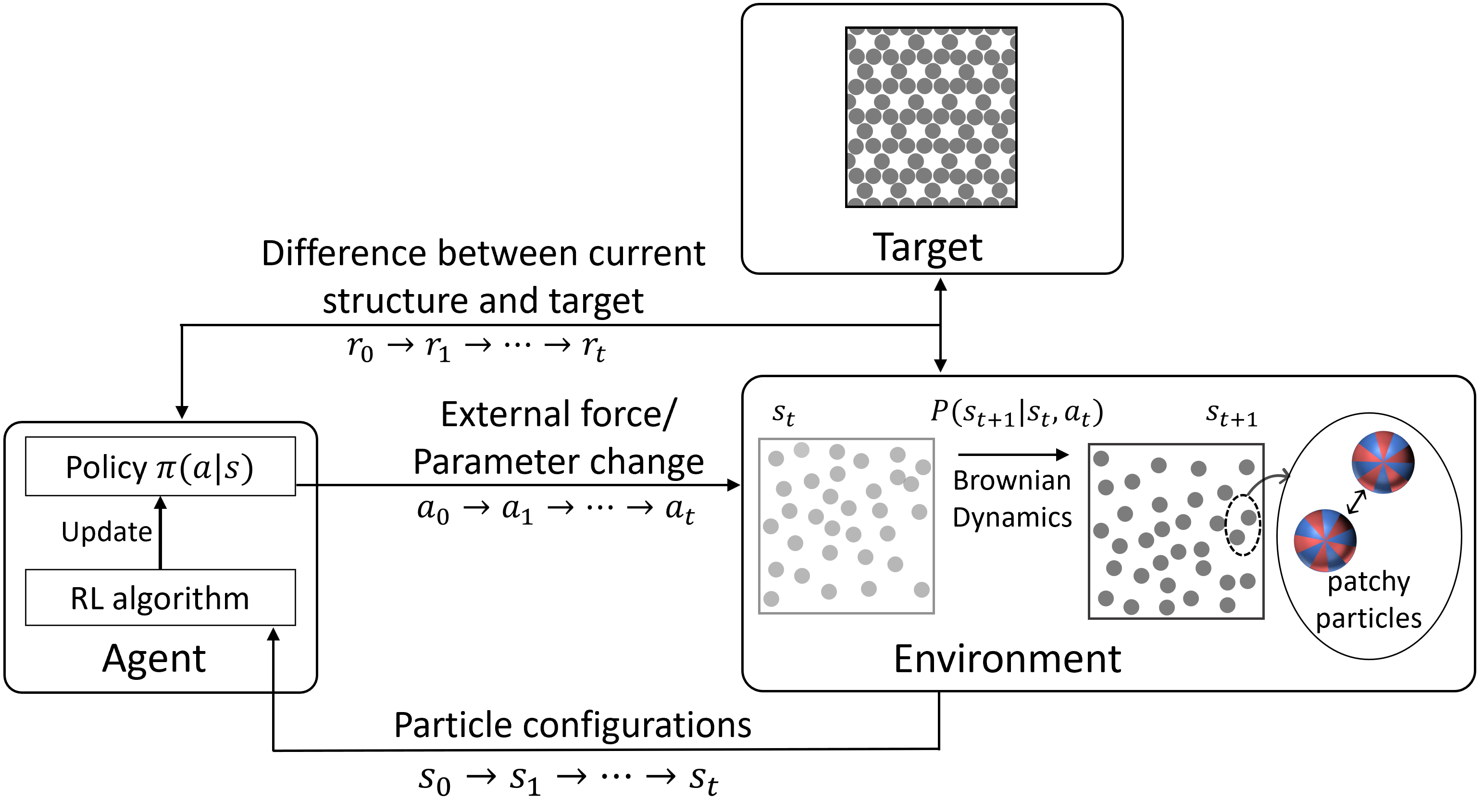
Fig.  1: Schematic of reinforcement learning for dynamic self-assembly. The agent observes the state $s$ from the environment, and decides to take an action $a$ based on the policy $\pi$. The agent learns the policy $\pi$ by a training process to optimise the rewards $r$. In this study, the environment is the particle configuration under a given temperature. The observed states are the ratio of sigma particle $\sigma$ and temperature $T$. The action is to decrease, maintain, or increase the current temperature.

2.1 Self-assembly of patchy particles through Brownian Dynamics simulations

Our system consists of $N$ patchy particles. Each particle stochastically moves and rotates following the equations (1) and (2) under the temperature $T$ at time $t$ (see Fig. 1). The patchy particle has anisotropic interactions with other particles. Depending on the anisotropy, the particles may form an ordered self-assembled structure. Because the thermal fluctuation of the particles is dependent on the temperature, the self-assembled structure varies as the temperature changes.

The Brownian dynamics (BD) simulation is employed to simulate the assembly of five-fold-symmetric patchy particles.^{13, 7} The patchiness on the spherical particle is described by the spherical harmonic of $Y_{55}$. There are 5 positive patches and 5 negative patches arranged alternatively around the particle’s equator (see Fig. 1). We set that the same sign patches are attractive while opposite patches are repulsive. The particles are confined to a flat plane, meaning that the particles can translate on the plane while they can rotate freely in three dimensions. In the Brownian dynamics, the position $\mathbf{r}$ and orientation $\bm{\Omega}$ of the particle are updated according to the equations

$$\mathbf{r}(t+\Delta t)=\mathbf{r}(t)+\frac{D^{\text{T}}}{k_{\text{B}}T}\mathbf{F}(t)\Delta t+\delta\mathbf{r},$$ (1)

$$\bm{\Omega}(t+\Delta t)=\bm{\Omega}(t)+\frac{D^{\text{R}}}{k_{\text{B}}T}\mathbf{T}(t)\Delta t+\delta\bm{\Omega},$$ (2)

where $D^{\text{T}}$, $D^{\text{R}}$ are the translational and rotational diffusion coefficients, respectively, $k_{\text{B}}$ is the Boltzmann constant, $\mathbf{F}$ and $\mathbf{T}$ are the force and torque, the Gaussian noise terms $\delta\mathbf{r}$ and $\delta\bm{\Omega}$ are with zero mean and satisfying $\langle\delta\mathbf{r}\delta\mathbf{r}^{\intercal}\rangle=2D^{\text{T}}\Delta t$ and $\langle\delta\bm{\Omega}\delta\bm{\Omega}^{\intercal}\rangle=2D^{\text{R}}\Delta t$, respectively. The characteristic length, energy, time, and temperature for the nondimensionalisation are the particle radius $a$, the potential well-depth $\varepsilon_{\text{V}}$, the Brownian diffusion time $\tau_{\text{B}}=a^{2}/D^{\text{T}}$, and $\varepsilon_{V}/k_{B}$, respectively.

The interaction potential of a pair of particles $i$ and $j$ is $V_{ij}=V_{\text{WCA}}(r_{ij})+V_{\text{M}}(r_{ij})\Xi(\bm{\Omega}_{ij})$. The isotropic Week-Chandler-Anderson term $V_{\text{WCA}}$ prevents the overlapping of particles. The interaction of the patchiness is given by the Morse potential $V_{\text{M}}$ and the mutual orientation dependent term $\Xi(\bm{\Omega}_{ij})$.

$$V_{\text{WCA}}=\begin{cases}4\varepsilon_{\text{V}}\left[(\frac{2a}{r})^{12}-(\frac{2a}{r})^{6}+\frac{1}{4}\right],&r\leq 2a\sqrt[6]{2}\\ 0,&r>2a\sqrt[6]{2}\end{cases}$$ (3)

$$V_{\text{M}}=\varepsilon_{\text{V}}M_{\text{d}}\left\{\left[1-e^{\left(-\frac{r-r_{\text{eq}}}{M_{\text{r}}}\right)}\right]^{2}-1\right\},$$ (4)

where $r$ is the center-particle distance; is the Morse potential equilibrium position, depth and range are respectively $r_{\text{eq}}=1.878a$, $M_{\text{d}}=2.294a$, and $M_{\text{r}}=a$. ³¹

The orientation of particle $i$ is determined by the orthogonal local bases $\hat{\bf n}^{(i)}_{m}$, $m=1,2,3$. Let $\hat{\bf r}$ be the unit distance vector of particle $i$ and $j$. The interaction of a pair of particle $Y_{lm}$ is $\Xi_{lm}\propto\{\hat{\bf n}_{0}^{l-m}\hat{\bf n}_{+}^{m}\}_{(i)}\odot\{\hat{\bf r}^{2l}\}\odot\{\hat{\bf n}_{0}^{l-m}\hat{\bf n}_{+}^{m}\}_{(j)}$, where $\hat{\bf n}_{0}=\hat{\bf n}_{3}$, $\hat{\bf n}_{+}=\frac{1}{\sqrt{2}}(\hat{\bf n}_{1}+i\hat{\bf n}_{2})$, and the $\{\}$ indicates the irreducible tensor. For a pair of $Y_{55}$ particles $\Xi_{55}\propto\{\hat{\bf n}_{+}^{5}\}_{(i)}\odot\{\hat{\bf r}^{10}\}\odot\{\hat{\bf n}_{+}^{5}\}_{(j)}$, and $\Xi$ is normalised to be in the range of [-1,1].

2.2 Reinforcement Learning and Q-learning

The basic ingredients of Reinforcement learning (RL) include an agent, an environment, and reward signals (Fig. 1). The agent observes the states $s$ of the environment and learns optimal actions $a$ through a policy $\pi$ that maximises the cumulative future rewards $R$.³² The future reward is the sum of the instantaneous reward $r_{i}$ at each step $i$

$$R =\sum_{i}\gamma r_{i},$$ (5)

with the discount factor $\gamma$. Formally, RL is expressed by a tuple of $\{\mathcal{S},\mathcal{A},\mathcal{P},g,\pi\}$ where $\mathcal{S}$ is a state space, $\mathcal{A}$ is an action space, $\mathcal{P}$ is a Markov transition process of the environment describing its time evolution, $g$ is the (instantaneous) reward function, and $\pi$ is a policy (Fig. 1). The transition process $P(s_{t+1}|s_{t},a_{t})\in\mathcal{P}$ maps the current state $s_{t}\in\mathcal{S}$ to the next state $s_{t+1}$ under the action $a_{t}\in\mathcal{A}$. The process is supplemented by the initial probability of the states $P(s_{0})$. The reward measures whether the current state is good or bad. The reward function gives some numbers from the current state and action as $r_{t}=g(s_{t},a_{t})$. In this work, we assume the reward function is dependent only on the state, that is, $r_{t}=g(s_{t})$. In general, the policy is a conditional probability $\pi(a|s)$ of taking the action under a given state. We assume the deterministic policy $a(s)$, namely, the action is the function of the state.

A physical interpretation of RL is to estimate the best dynamic control strategy to get a desired structure or physical property (see Fig. 1). The physical system of variables $s_{t}$ yields the dynamics expressed by the Markov process $\mathcal{P}(s_{t+1}|s_{t},a_{t})$ under an external force and/or parameter change in the model expressed by $a_{t}$. At each time, we can compare the current state $s_{t}$ and the target state $s^{*}$. The distance between them is an instantaneous reward. The goal of RL is to estimate the best policy from which we choose the action $a$ as a function of the current state $s$.

In the context of self-assemblies, RL aims to control the external force or the parameters so that the desired structure is organised from a random particle configuration. In this study, we control temperature; our action is whether temperature increases, decreases, or stays at the current value. The environment is the configuration of the particles at certain conditions, such as temperature and density. In principle, the dimension of the state space is huge. It may be all the degrees of freedom of the particles, their positions and orientations. Nevertheless, our purpose is to make the desired structure, which is the DDQC structure. Therefore, we use statistical quantities (or feature values) to characterise the particle configurations. This is the number of $\sigma$ particles, denoted as $N_{\sigma}$; we will discuss this issue in detail in Sec. 2.3. We consider two observed states from the environment: the temperature $T$ and the ratio of $\sigma$ particles of the DDQC, which is extracted from the particle configuration, to the total particles. We denote the ratio by $\sigma=N_{\sigma}/N$. From the observed states, we take an action $a$ updating the current temperature to the next one. We also get a reward $r_{t}$ from the measured state. From the reward, the next action is decided at each step and the procedure continues to update all different states. Within each step, the configuration of particles is updated by BD simulations.

There are many RL algorithms to train the agent. Q-learning is a popular algorithm for learning optimal policies in Markov decision processes.³³ It is a model-free, value-based algorithm that uses the concept of Q-values (Quality value) to guide the agent’s decision-making process. Q-value, denoted as $Q(s,a)$, is the cumulative reward obtained by taking action $a$ on the current state $s$ and then following the optimal policy. The simplest Q-learning uses a Q-table in which Q-values are updated at each point in discretised action and state spaces. The size of Q-table depends on the number of elements of the state spaces and action spaces. For example, consider a system with two state spaces discretised into $m$ and $n$ elements, and an action space with $l$ elements. In this case, the corresponding Q-table is a three-dimensional array with dimensions $m\times n\times l$. This array represents the whole state-action space, in which the agent (we) can store and update Q-values for all possible combinations of states and actions. The policy is then extracted from the Q-value of each state-action pair $Q(s,a)$. In general, the algorithm involves many epochs (or episodes). The Q-table is initialised at first. For each epoch, the states are also initialised, then for each step in the epoch, we perform the following algorithms:

• Observe a current state $s_{t}\in\mathcal{S}$.

• Select and perform an action $a_{t}\in\mathcal{A}$ based on the policy from $Q(s,a)$.

• Observe the subsequent state $s_{t+1}$.

• Receive an immediate reward $r_{t+1}$.

• Update iteratively the Q-function by

$$Q(s_{t},a_{t})=Q(s_{t},a_{t})+\alpha[r_{t+1}+\gamma\max_{a}Q(s_{t+1},a)-Q(s_{t},a_{t})],$$ (6)

where the learning rate $\alpha$ is a hyperparameter $0\leq\alpha\leq 1$ that reflects the magnitude of the change to $Q(s_{t},a_{t})$ and the extent that the new information overrides the old information. If $\alpha=0$, no update at all; if $\alpha=1$, then completely new information is updated in $Q$. The discount factor $\gamma$ is associated with future uncertainty or the importance of the future rewards $(0\leq\gamma\leq 1)$.

In RL, it is important to consider the balance between exploitation and exploration. If we just follow the current (non-optimal) policy, it is unlikely to find potentially more desired states. On the other hand, if our search is merely random, it takes a significant amount of time to find them. In Q-learning, exploitation involves selecting the action that is believed to be optimal, i.e. maximum Q-value, while exploration involves selecting the action that does not need to be optimal within the current knowledge. To balance these strategies, the $\epsilon$-greedy method is used. In the $\epsilon$-greedy method, a random action at each time step is selected with a fixed probability $0\leq\epsilon\leq 1$ instead of the optimal action with respect to the Q-table.

$$\pi(s)=\begin{cases}\text{random action }a\in\mathcal{A},&\text{if }\xi<\epsilon\\ \operatorname*{arg\,max}_{a\in\mathcal{A}}Q(s,a),&\text{otherwise,}\end{cases}$$ (7)

where $0\leq\xi\leq 1$ is a uniform random number at each step.

2.3 Characterisation of DDQC structures

One method to characterise two-dimensional DDQC is to determine local structure around each particle according to its nearest neighbours ^{16, 34, 7} (Fig. 2). Given the particle positions, the sigma, hexagonal $Z$, and $H$ local structures are estimated. A DDQC structure usually contains a few $Z$ dispersed in many sigma and a few $H$ particles. In detail, dodecagonal motif, which is made from one centred $Z$ and 18 sigma particles (Fig. 2d), is observed in the DDQC. The motifs can be packed in different ways, e.g. the centres form triangles. The ratio of the sigma, Z, and H particles to the total particles in the packed motifs are found to be $0.8\leq\sigma\leq 0.93$, $0.07\leq Z\leq 0.14$, and $0\leq H\leq 0.13$, respectively. Such ratios are found comparable to those in simulated DDQC^{16, 7} or square-triangle tiling.³⁵ In our simulations, the value of $\sigma=N_{\sigma}/N$ ($N_{\sigma}$ is the number of sigma particles) is observable and it can express the quality of a DDQC; therefore we choose $\sigma$ as one of the states of the RL ($0\leq\sigma\leq 1$). The value $\sigma^{*}$ of the target DDQC is set as $\sigma^{*}=0.91$. To obtain more complex structures, other quantities, such as the number of Z particles, may be needed. However, as we demonstrate, using only $\sigma$ works well for DDQC for different models as well as for other targets (see Sec. 3.3 and 3.4).

Ideally, the ratio of the sigma particles to the total particle in DDQCs is expected to be around $0.8\leq\sigma\leq 0.93$. However, at finite temperatures, defects can always appear during the self-assembled process. The structures with defects are frozen and form metastable states. We consider that structures with $\sigma\gtrsim 0.7$ are global minimum DDQCs with a few defects. On the other hand, when $0.5\leq\sigma\leq 0.7$, there are more defects in the structures and we refer to them as metastable states. The metastable and global minimum structures distinguished by the value of $\sigma$ are demonstrated in their Fourier transformation images, showing distinguishable 12-fold symmetry spots from the background (Fig. 2).

Another state used in RL is the temperature $T$. The range of the temperature is chosen as $0.2\leq T\leq 1.3$ so that the particle interaction dominates the noise at $T_{\text{min}}$ and the noise dominates the interaction at $T_{\text{max}}$.

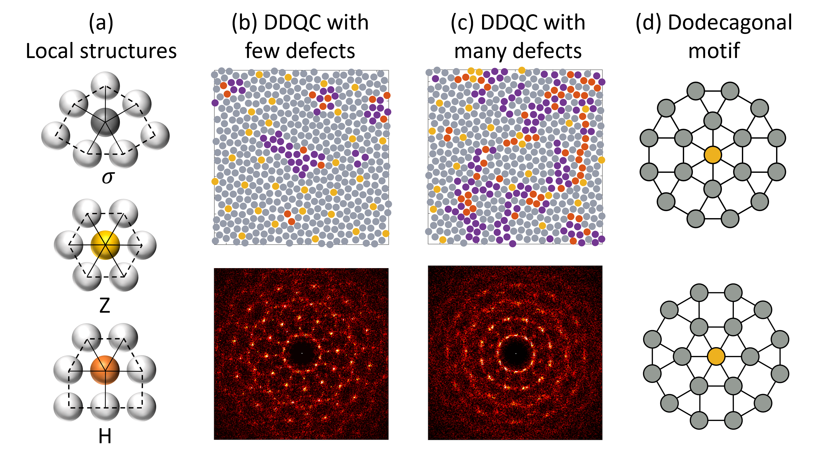
Fig.  2: Characterisation of DDQCs. (a) Demonstration of local structures. (b-c) Examples of DDQC with few and many defects, and the correspondent Fourier transformations. The defect points are marked purple. The fraction of sigma in (b-c) are 0.84 and 0.67, respectively. (d) Dodecagonal motif made from one $Z$ particle centred in 18 $\sigma$ particles.

2.4 Reinforcement learning for dynamic self-assembly

The schematic for Q-learning in this study is given in Fig. 3. Initially, Q-table is set to zero for all $a$ and $s$. The RL includes $N_{\text{e}}$ epochs or episodes in which the $\epsilon$-greedy method is applied. In each epoch, the initial state, i.e. the initial particle configuration and the initial temperature $(\sigma_{0},T_{0})$ are assigned. Next, the action $a_{0}$ (either decrease, maintain, or increase $T$) for the temperature is decided based on the current policy and the $\epsilon$-greedy strategy, resulting in the new temperature $T_{1}$. The Brownian dynamics simulation for the current particle configuration at $T_{1}$ is conducted. Details of the Brownian dynamics simulation can be found in Sec. 2.1. The new particle configuration is obtained after a predetermined time $t=N_{\text{BD}}\Delta t$. Then one can determine the state $\sigma_{1}$, the reward $r_{1}$, and eventually update the $Q$-value $Q(\sigma_{0},T_{0},a_{0})$. This concludes the Q-learning of the first step. The next step can be conducted analogically from the current state $(\sigma_{1},T_{1})$. The Q-table is updated at every action step, every epoch, until the training process ends.

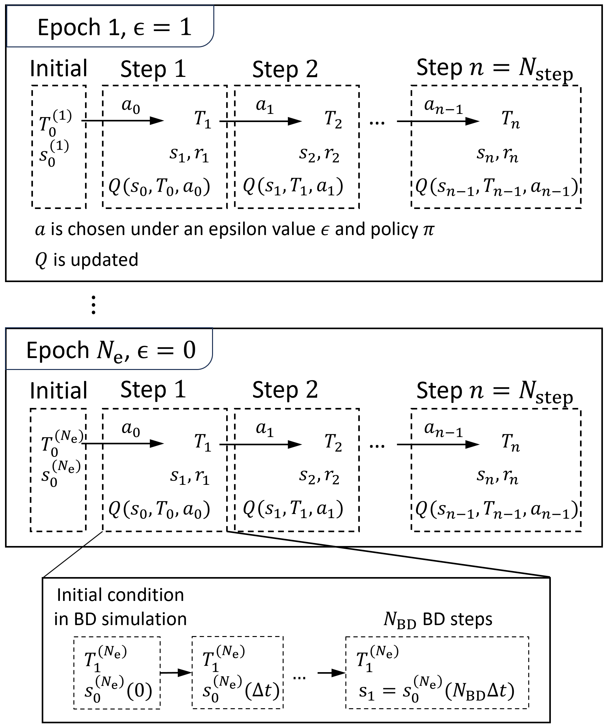
Fig.  3: Schematic of Q-learning at each epoch with $\epsilon$-greedy method. The action $a$ is chosen based on the current policy $\pi$ and $\epsilon$. Q is updated according to eq. (6). Brownian dynamics (BD) simulation is conducted for every step in $N_{\text{step}}$ of each epoch.

From the trained Q-table, we can estimate the policy on controlling the temperature with respect to the current state. In order to evaluate the estimated policy, 20 independent tests are conducted. Each test starts with an assigned initial particle configuration and temperature (initial states), followed by consecutive steps of deciding the next action based on the estimated policy, observing the new states, and so on. Otherwise stated, we set the parameters the same as the parameters used during training, except that $\epsilon=0$ is fixed in every test.

Table 1 shows the parameters of a training set for the target DDQC from patchy particles. The two observed states are the ratio of sigma particle $\sigma$ and the temperature $T$. Initially, the configuration of the particle is random (corresponding to $\sigma_{0}<0.1$) and $T_{0}$ values are chosen randomly in the investigated range. While the fraction of sigma never reaches out of the range $[0,1]$, the temperature $T_{k+1}$ after the action $a_{k}$ may exceed the investigated range. In this case, the updating is carried out as usual except that we treat $T_{k+1}=T_{k}$. The policy after training is used for the test at the same conditions as training (except $\epsilon$).

Parameter	Value
States of sigma fraction, $\sigma$	$[0,1]$, intervals of 0.1
States of temperature, $T$	$[0.2,1.3]$, intervals of 0.1
Actions on the temperature, $a$	$\{-0.05,0,0.05\}$
Number of epochs, $N_{\text{e}}$	101
$\epsilon$-greedy	Linearly decrease in each epoch
	from 1 to 0
Initial temperature at each	Random $\in[0.2,1.3]$
epoch, $T_{0}$
Initial structure at each	Random ($\sigma_{0}<0.1$)
epoch, $\sigma_{0}$
Number of action steps in each	200
epoch, $N_{\text{step}}$
Number of BD steps in each	$100,000$ steps equivalent
BD simulation, $N_{\text{BD}}$	to $t=10$
Target, $\sigma^{*}$	0.91
Rewards, $r$	$-(\sigma-\sigma^{*})^{2}$
Learning rate, $\alpha$	0.7
Discount factor, $\gamma$	0.9
Number of particles, $N$	256
Area fraction	0.75

Table 1: [RL1] Parameters for the training set of DDQC patchy particles.

2.5 Q-learning for triple-well potential model

In RL for the DDQC self-assembly, the biggest challenge is how to avoid the metastable states and reach the global minimum state by controlling the temperature. In order to show how RL works to overcome the energy barriers between the disordered, metastable and DDQC structures, we consider a simple model in which a single particle at the position $x$ moves in a temperature-dependent triple-well potential. We design the model such that the states $x$ and $T$ correspond to $\sigma$ and $T$ of DDQC self-assembly, respectively. Similar to the DDQC, we apply Q-learning for a model consisting of two state variables $x$ and $T$. The states follow the dynamics described by the following Langevin equations

$$x(t+dt)= x(t)-\partial_{x}U(x,T)dt+\xi_{x}$$ (8)

$$T(t+dt)= T(t)+a+\xi_{T}.$$ (9)

The state $x$ moves in the $T$-dependent potential $U(x,T)$, whereas $T$ evolves through the action $a$ with noise. The functional form of the potential is shown in Fig. 8. The fluctuation of $x$ is illustrated by the noise term $\xi_{x}$. The relation of $x$ and $T$ is described by a triple-well potential $U(x,T)=-\frac{1}{\tau}\sum_{i=1}^{3}\mathcal{N}_{i}(x;\mu_{i},\sigma_{\text{p}i})h_{i}(T)$ where $\mathcal{N}_{i}(x;\mu,\sigma_{\text{p}i})$ is the Gaussian distribution with mean $\mu_{i}$ and standard deviation $\sigma_{\text{p}i}$, $h(T)$ is a temperature dependent function. By designing $\mathcal{N}_{i}(x;\mu_{i},\sigma_{\text{p}i})$ and $h_{i}(T)$, the position and the depth of the well can be controlled. The parameter of each well is $\mu_{1}=0.16$, $\sigma_{\text{p}1}=0.2$, $h_{1}(T)=T^{2}$, $\mu_{2}=0.55$, $\sigma_{\text{p}2}=0.11$, $h_{2}(T)=(1.5-T)^{4}$, $\mu_{3}=0.88$, $\sigma_{\text{p}3}=0.11$, $h_{3}(T)=1.8(1.4-T)^{4}$. With the choice of parameters, our triple-well potential has minima at $x=\mu_{1},\mu_{2},\mu_{3}$. The potential minimum at $x=\mu_{1}$ is shallow, whereas the potential minima at $x=\mu_{2},\mu_{3}$ are deeper. The global minimum at the low $T$ is $x=\mu_{3}$, but there is a large energy barrier between $x=\mu_{2}$ and $x=\mu_{3}$ at low $T$ so that the transition from $x=\mu_{2}$ to $x=\mu_{3}$ is unlikely. The shape of the potential for different temperatures is shown in Fig. 8(a). We design the triple-well potential to imitate the disordered state in the self-assemblies of DDQC by $x=\mu_{1}$, and the metastable state ($\sigma\approx 0.6$) and the global minimum ($\sigma\approx 0.8$) correspond to $x=\mu_{2}$ and $x=\mu_{3}$, respectively.

We set $\tau=500$, $dt=1$, and $\xi_{x}$ following a normal distribution with mean zero and standard variation of 0.022. The parameters during the training of RL are chosen to be the same as the case for the DDQC given in Table 1, except that at each $T$, the number of update steps is set to 1000.

2.6 Summary of the investigated RL

Here, we summarise the four RL systems studied in this work in Table 2. In [RL1], we focus on the details of RL for the formation of DDQC using patchy particles. Then, we explain how RL overcomes the energy barriers to reach the global minimum using the model of a triple-well potential [RL2]. To show the generality of proposed RL, in [RL3], we demonstrate that RL can estimate the policy for DDQC formation from particles interacting through a two-lengthscale isotropic potential. It is known that this model also exhibits DDQC.³⁶ Details of the isotropic potential can be found in Ref.⁷ and the references therein. The purpose of [RL3] is to show the versatility of RL and insights into different physical systems from the estimated policy. Finally, by changing the target structures in [RL4], we demonstrate that RL is capable of stabilising a metastable structure ($\sigma^{*}=0.65$) and even finding a policy to control structure dynamically to realise the unstable target structure ($\sigma^{*}=0.35$).

	RL1	RL2	RL3	RL4
Method	Q-table	Q-table	Q-table	Value Iteration
Model	Patchy	Triple-well	Isotropic	Patchy
Target	$\sigma^{*}=0.91$	$x^{*}=0.90$	$\sigma^{*}=0.91$	$\sigma^{*}=0.65$,
	(DDQC)	(global minimum)	(DDQC)	$\sigma^{*}=0.35$

Table 2: Four systems studied using RL in this work. The RL method, physical model, and target of each system are shown. In [RL4], we use Value Iteration^{32, 37} to estimate Q function and policy. Details of this method can be found in Appendix A.

3 Results

3.1 Optimal temperature change to generate DDQC from patchy particles [RL1]

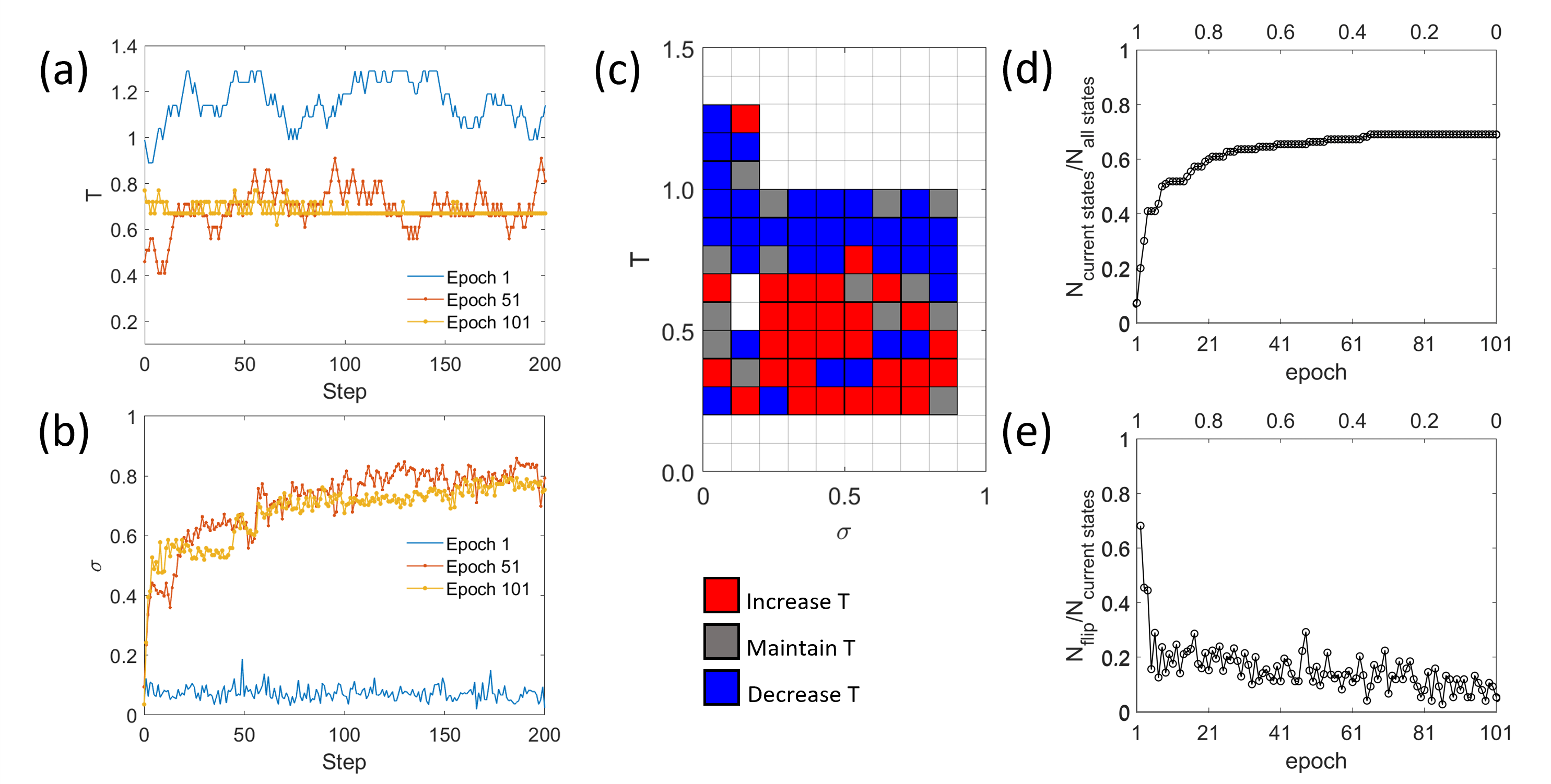
Fig.  4: [RL1] Training data at the condition of random $T_{0}$ and number of epochs $N_{\text{e}}=101$ in Table 1. (a,b) The progression of the states $T$ and $\sigma$ at selected epochs: first, middle and last epoch (equivalent $\epsilon=0,0.5,1$ respectively); (c) the policy after training; (d) the change of ratio of the number of accessed states to total states and (e) ratio of flipped-policy states to accessed states after each epoch during training, the horizontal axis on the top of the graph is the corresponding value of $\epsilon$.

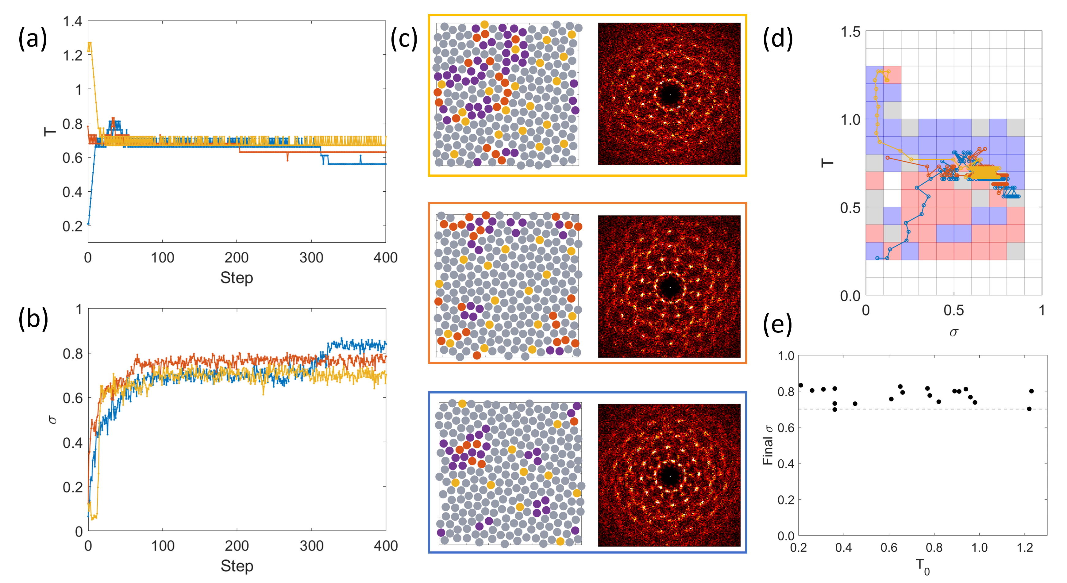
Fig.  5: [RL1] Testing data of the policy obtained at the condition of random $T_{0}$ and number of epochs $N_{\text{e}}=101$ in Fig. 4. Samples starting with different initial temperatures are shown with (a) the temperature schedule, (b) corresponding $\sigma$, and (c) snapshots at the last step of the corresponding trajectories. (d) The trajectories of (a,b) on the policy plane obtained from Fig.4(c), in which the starting points are from the left side. Changes of temperatures of the trajectories follow the policy shown in the background. (e) The dependence of $\sigma$ on the initial temperature $T_{0}$ obtained from 20 individual samples. The dashed line is a guide to the eye for the lower limit of global minimum DDQCs.

First, we demonstrate the capability of Q-learning to find the best temperature schedule to create DDQCs of patchy particles from random configurations. Figure 4 shows the training result under the condition in Table 1, where the policy is trained with $N_{\text{e}}=101$ epochs and the initial temperature $T_{0}$ at each epoch is randomly selected within the investigated range. At each epoch, the action changes according to the current policy and $\epsilon$, hence the states of temperature and $\sigma$ change at each step, as shown in Fig. 4(a-b). At the first epoch in which $\epsilon=1$, the action is random and $T$ fluctuate around $T\approx 1.0$. Accordingly, $\sigma$ is low $\sigma<0.2$ and far from the target value $\sigma^{*}$. As the training continues, Q-table is updated. At the mid epoch $n=51$ at which $\epsilon=0.5$, $T$ fluctuates around $T\approx 0.7$ whereas at the last epoch $n=101$ at which $\epsilon=0$, $T$ shows less fluctuation around $T\lesssim 0.7$. After the epoch $n=51$, $\sigma$ approaches closer to $\sigma^{*}$.

Figure 4(c) demonstrates the policy after training, which is the action for the maximum of $Q$, namely, $\operatorname*{arg\,max}_{a}Q{\color[rgb]{0,0,0}}$. This state-space roughly consists of two regions divided by a critical temperature $T^{*}=0.7$. The estimated policy is to decrease the temperature above $T^{*}$, and to increase the temperature below $T^{*}$. When $\sigma\geq 0.8$, the temperature can be decreased further to $T\approx 0.5$. The action of ‘maintaining temperature’ can be seen in the policy, but no clear correlation to the states is observed. The policy has states that are not accessed during training. The action for these inaccessible states is random. Figure 4(d) presents the ratio of the number of accessed states to total states during training (total number of states is $10\times 11$). We also measure whether the policy converges to its optimal in Fig. 4(e), by defining the ratio of the number of flipped states to accessed states. The flipped state is counted when the policy at the current epoch $\pi^{(i)}(s,a)$ changes compared to the policy at the previous epoch $\pi^{(i-1)}(s,a)$. The ratio decays to $\lesssim 0.1$, but the decay is slow. Even after the epoch of $\epsilon\lesssim 0.4$ after which the number of accessed states reaches a plateau, the ratio is still decaying slowly. This result suggests that many epochs are required to reach an optimal policy.

After training, the estimated policy is tested. The results of the test are presented in Fig. 5. The time evolution of temperature and $\sigma$ during the test with initial configurations of random particle positions and orientations and with random $T_{0}$ are shown in Fig. 5(a,b). At first, $T$ quickly reaches the critical temperature $T\approx 0.7$, then fluctuates around that value until $\sigma$ reaches the target value. Finally, $T$ decreases at a considerably slower rate to $T\approx 0.6$. The final temperature is dependent on each realisation; in some cases, $T$ reaches $T\approx 0.6$, whereas, in other cases, $T$ stays at $T\approx 0.7$. Correspondingly, the final value of $\sigma$ is either $\sigma\approx 0.8$ or slightly smaller than that. The snapshots at the final steps have dodecagonal motifs consisting of one $Z$ particle centred in 18 $\sigma$ particles (see Fig.2(d)). The intensities in the Fourier space show clear twelve-fold symmetry, although some defects are present in the real space.

Figure 5(d) shows trajectories of the states ($T$ and $\sigma$) during the test together with the estimated policy. We show the three trajectories with different initial temperatures: high $T_{0}$, intermediate $T_{0}$, and low $T_{0}$. In the case of high $T_{0}$, the temperature decreases to $T\approx 0.{\color[rgb]{0,0,0}}$ but $\sigma$ does not increase. Once the temperature becomes $T\approx 0.7$, dodecagonal structures start to appear and $\sigma$ increases and fluctuates around $\sigma\approx 0.7$.

In the case of low $T_{0}$, some dodecagonal structures appear from the beginning because the temperature is low. As the temperature is increased to $T\approx 0.7$, $\sigma$ is also increased and reaches $\sigma\approx 0.7$. The temperature is found to decrease at the point $\sigma\approx 0.8$.

When the initial temperature $T_{0}$ is intermediate, $\sigma$ is increased, then fluctuates, and finally, it is increased more when $T_{0}$ is decreased slightly. Note that in all cases, the initial $\sigma$ is small because the initial configuration of particles is random in position. Using this policy, the DDQC structure can be obtained in tests at any value of the initial temperature $T_{0}$ (Fig. 5(e)). In short, the RL agent has found out the role of the critical temperature $T^{*}$ in facilitating the formation of the DDQC structure. As a result, when the DDQC is not formed (low $\sigma$), the RL suggests to drive the temperature to this critical until a DDQC (high $\sigma$) is formed. Then decrese $T$ to stabilise the structure. It is noted that the RL discovers the critical temperature by itself. We do not feed any information about the role of $T^{*}$ or its value. The role of $T^{*}$ is in contrast with the results for the system with the isotropic interactions, discussed in Sec. 3.3.

Next, we compare the formation of a DDQC using the estimated policy with the self-assembly using the conventional annealing method.⁷ Figure 6 shows the trajectories of $T$ and $\sigma$ for different realisations. In the case of the annealing, we have used the linear temperature decrease in BD steps. In this case, the time step for each BD step was also decreased for numerical stability. In both methods, $\sigma$ values reach $\sigma\approx 0.8$, at which the dodecagonal structures appear clearly with a few defects. In the case of the annealing, we have used a pre-fixed temperature schedule, and therefore, $t\gtrsim 2000$ is required for the dodecagonal structures. On the other hand, by using the estimated policy, we can get comparable structures in a much faster time. We should stress that when the slope of the temperature change is sharper for the pre-fixed schedule (which is referred to as quenching), the structure is trapped at the metastable state and the DDQC with few defects cannot be generated.⁷

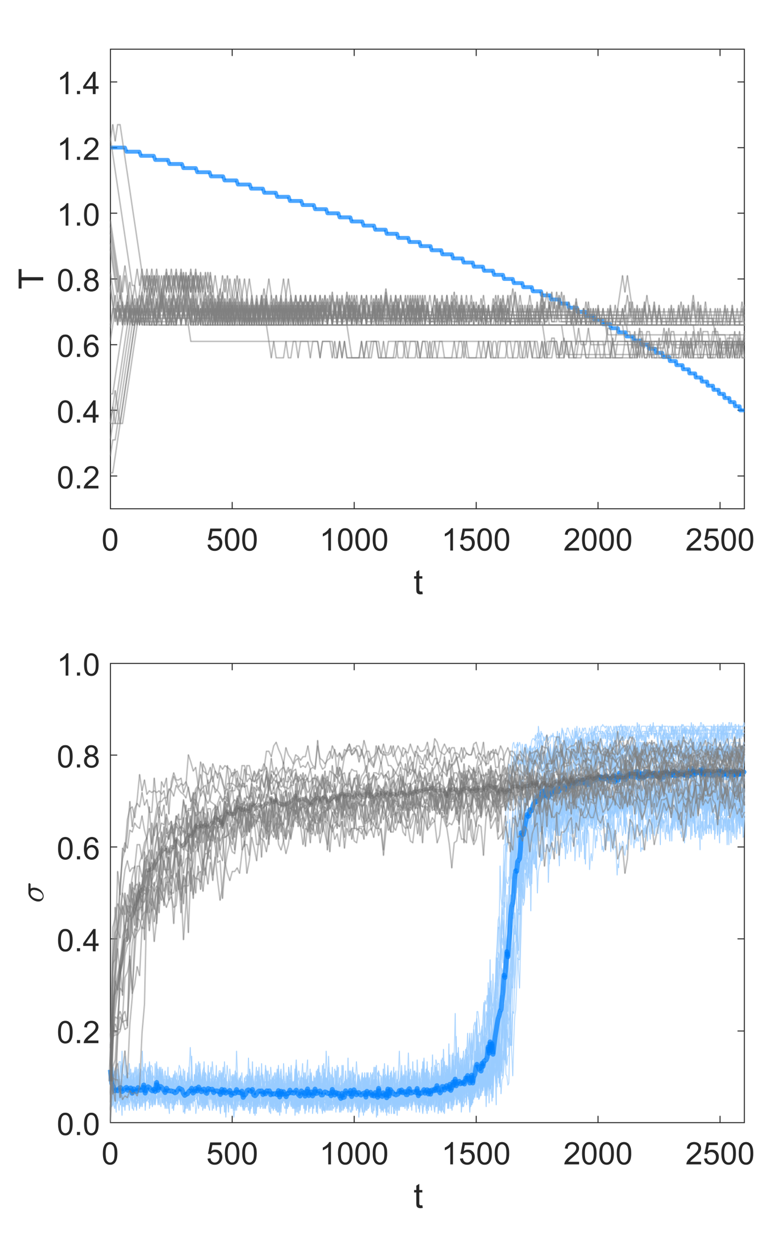
Fig.  6: [RL1] Comparing DDQC assemblies by RL temperature policy and annealing. The thin lines are the temporal changes of temperature and ratio of sigma of RL testing (grey) and annealing (blue) samples. The bold lines are the mean values of $\sigma$.

We use a smaller system size, $N=256$, in the training steps. It is important to check whether the estimated policy using RL can work upscale. We perform the test at larger system sizes $N=512$ and $N=1024$. Figure 7 demonstrates the statistics of the obtained structure of different system sizes. The estimated policy for the smaller systems size works even for the tests with all investigated system sizes, namely, we obtain $\sigma\gtrsim 0.7$. The mean value of $\sigma$ seems to slightly decrease with system size. This is because the larger system size requires more time to stabilise. If more steps are conducted for a larger system size, there is no significant difference difference the three groups. In fact, the snapshots both in the real and Fourier spaces for the larger system sizes show dodecagonal structures.

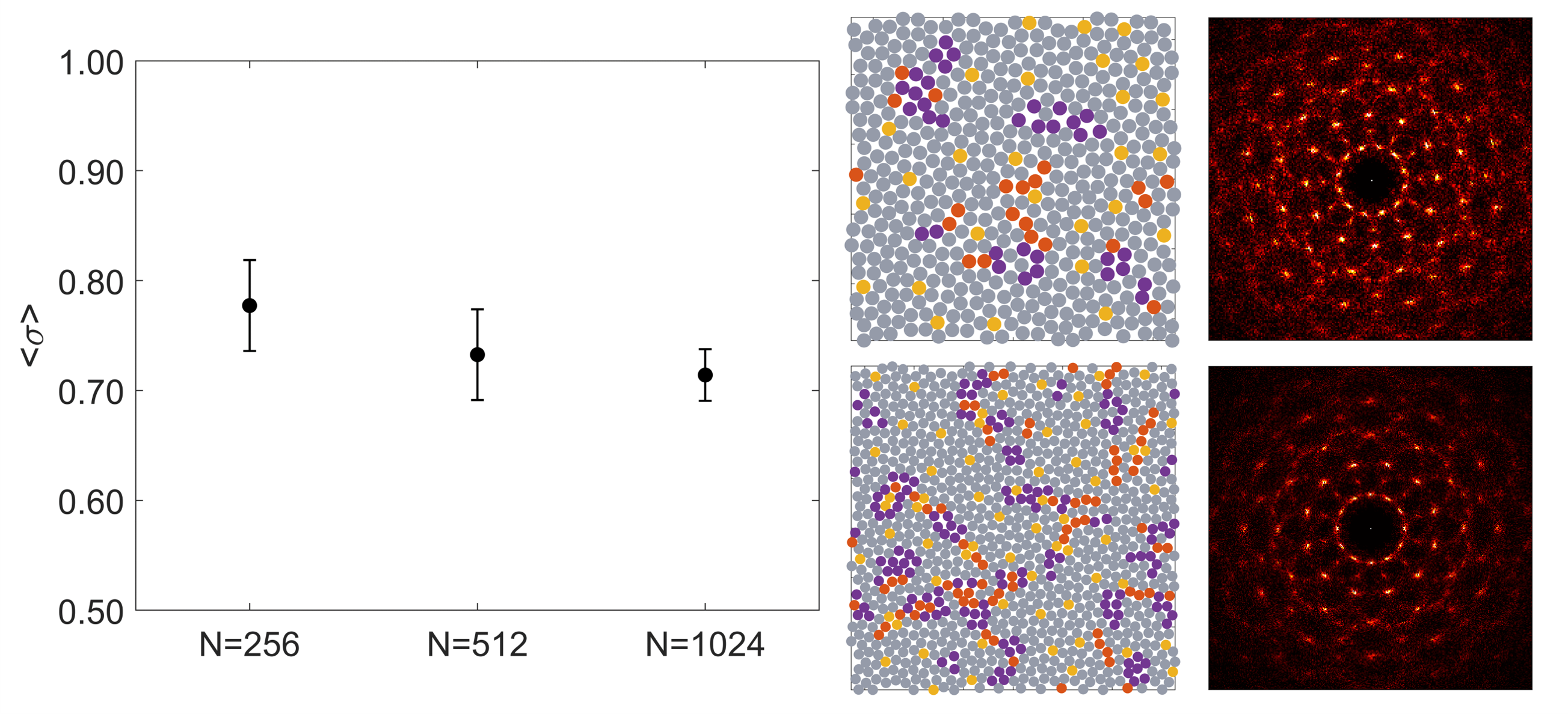
Fig.  7: [RL1] Performance of the testing on different system sizes, where the policy is trained with the system of $N=256$ particles. The means and standard deviations are calculated from 20 independent samples. The snapshots and Fourier transformations are demonstrated for $N=512$ (upper) and $N=1024$ (lower) tests.

3.2 Reinforcement learning for a simple model [RL2]

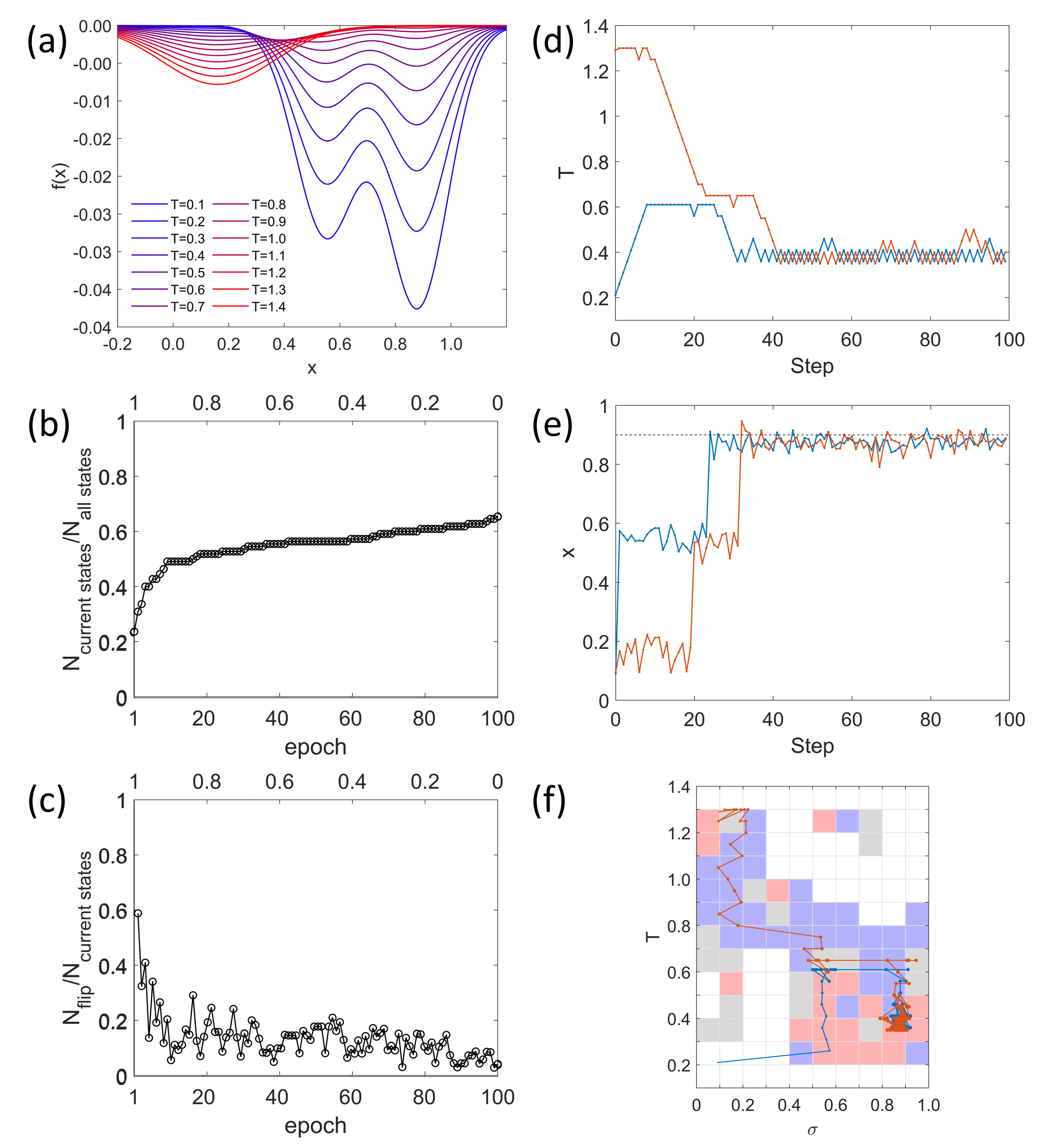
Fig.  8: [RL2] Q-learning for the simple model trained with random $T_{0}$ and number of epochs $N_{\text{e}}=100$. (a) The triple-well potential. (b) The ratio of the number of accessed states to total states and (c) the ratio of flipped-policy states to accessed states during training. (d-e) The states $T$ and $x$ of two independent samples and (f) their trajectories on the policy plane, noting that the point size increases with the step.

To get a deeper insight into the mechanism of RL for DDQC formation, we apply Q-learning for a simple model. In this model, the state $x$ (analogical to the state $\sigma$ of DDQC) evolves under the triple-well potential shown in Fig. 8(a). We design the dependence of $x$ on the temperature analogous to that of $\sigma$ in DDQC. At high temperature, the local minimum is at $x=0.16$, similar to the low $\sigma$ structure. As the temperature decreases, this local minimum disappears, and two additional local minima appear at $x=0.55$ and $x=0.88$. The former value imitates the metastable state of a DDQC with many defects, whereas the latter corresponds to DDQC with fewer defects. By introducing the noise, a state $x$ can jump from one well to the other well under intermediate temperature $T$.

The results of the training and testing are given in Fig. 8. We use the number of epochs $N_{\text{e}}=100$ and the random initial $T=T_{0}$ at the beginning of each epoch. Figure 8(b,c) shows the ratio of the number of accessed states and the convergence of the policy during training of the Q-table. As the number of epochs increases (from $\epsilon=1$ to $\epsilon=0$), the number of accessed states increases, and the flip ratio converges slowly toward zero. Figure 8(d-f) depicts the time evolution of the states $T$ and $x$ of two testing samples and their trajectories on the policy plane. Starting with either a high or low value of $T_{0}$, the temperature quickly reaches $T\approx 0.6$, at which $x$ fluctuates around the middle local minimum $x=0.55$. After some time, $T$ further decreases to a lower value $T\approx 0.4$, and accordingly, $x$ goes to the deepest well. The estimated policy suggests two regions: decrease $T$ when $T>0.6$ and increase $T$ when $T<0.6$. The boundary between the two regions is analogical to the critical temperature for the DDQC case.

3.3 Reinforcement learning for DDQC of isotropically interacting particles [RL3]

In this section, we perform RL for target DDQC assembled by particles interacting with the isotropic potential. The purpose is to show the versatility of RL in handling different physical systems. As shown in Fig. 9, the trained policy for the DDQC target from particles with isotropic interactions has many ’blue’ and ’grey’ elements at $T\geq 0.4$, which suggests that just decrease the temperature to $T\approx 0.4$. This result is in contrast with that of patchy particles shown in Sec. 3.1. For the isotropically interacting particles, simpler temperature protocol without critical temperature works for the DDQC formation.

For the test starting from high initial temperature $T_{0}\approx 1.2$, the temperature rapidly decreases to $T=0.5$. When the temperature passes through $T=0.8$, the particles quickly assemble into a DDQC structure whose $\sigma\approx 0.8$. The test of low initial temperature $T_{0}\approx 0.3$ shows that even at such a low temperature, the structure of $\sigma\approx 0.75$ can be formed immediately. Then, the policy suggests keeping $T\approx 0.4$ so that the quality of the DDQC can be improved as $\sigma>0.8$. Compared to the DDQC of patchy particles, the RL, in this case, does not feel about the existence of a critical temperature $T^{*}$ although $\sigma$ increases drastically as $T\approx 0.8$. The agent learns through training that, for isotropic particles, the complex temperature protocol, as we have seen for the patchy particles, is not necessary to make the DDQC without defects.

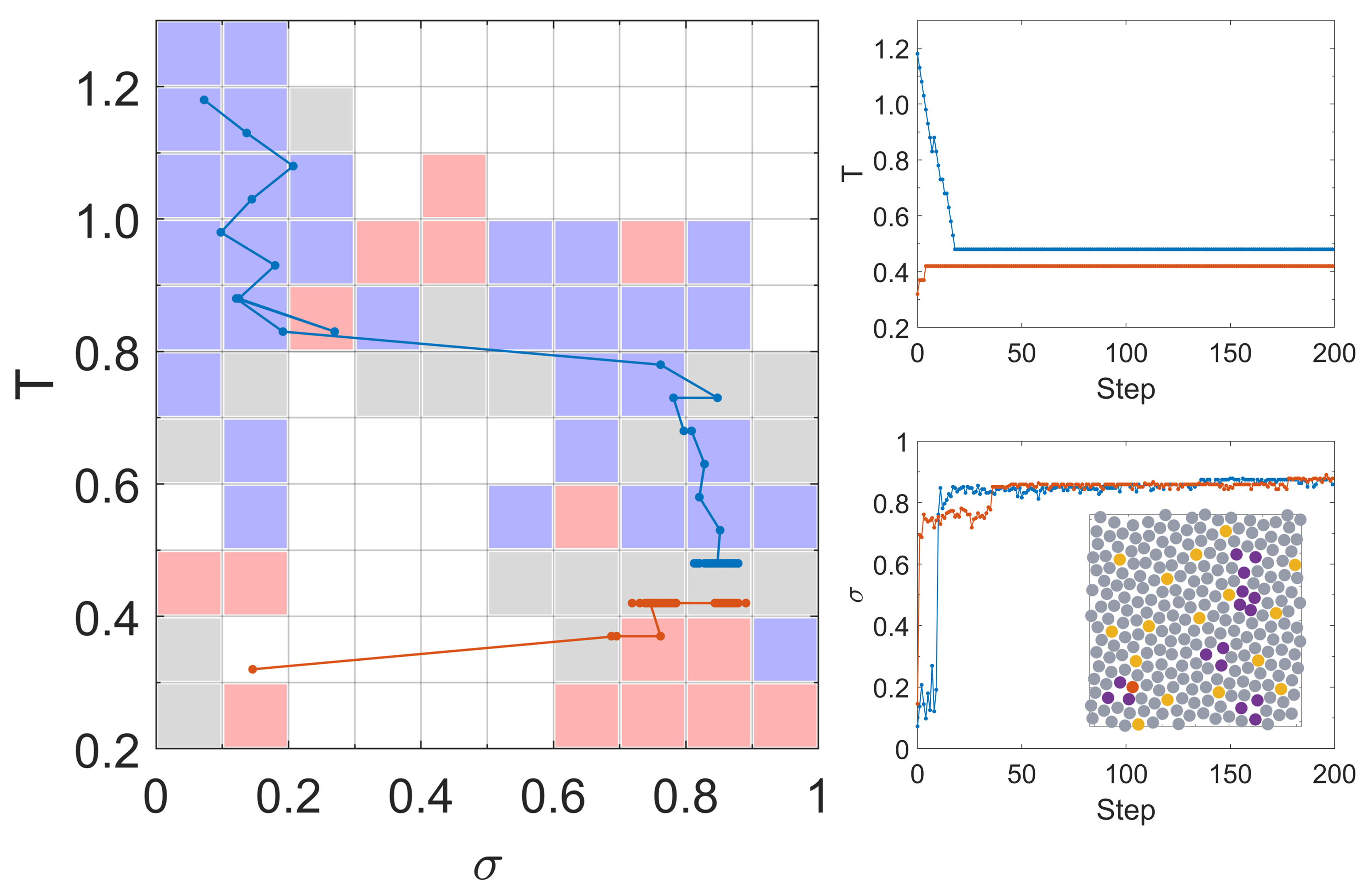
Fig.  9: [RL3] Reinforcement learning for DDQC of isotropically interacting particles. (Left) The trained policy with selected trajectories during tests and (right) the corresponding temperature and $\sigma$ of the tests. The mean and standard deviation of $\sigma$ from 20 independent samples are 0.84 and 0.03, respectively. The snapshot at the last point of the (orange) trajectory is given. The training condition for the isotropic particle system is the same as that of the patchy particle system in Table. 1 except that the number of steps of each epoch is $N_{\text{step}}=100$ and the area fraction is 0.81.

3.4 Reinforcement learning for unknown targets of patchy particles [RL4]

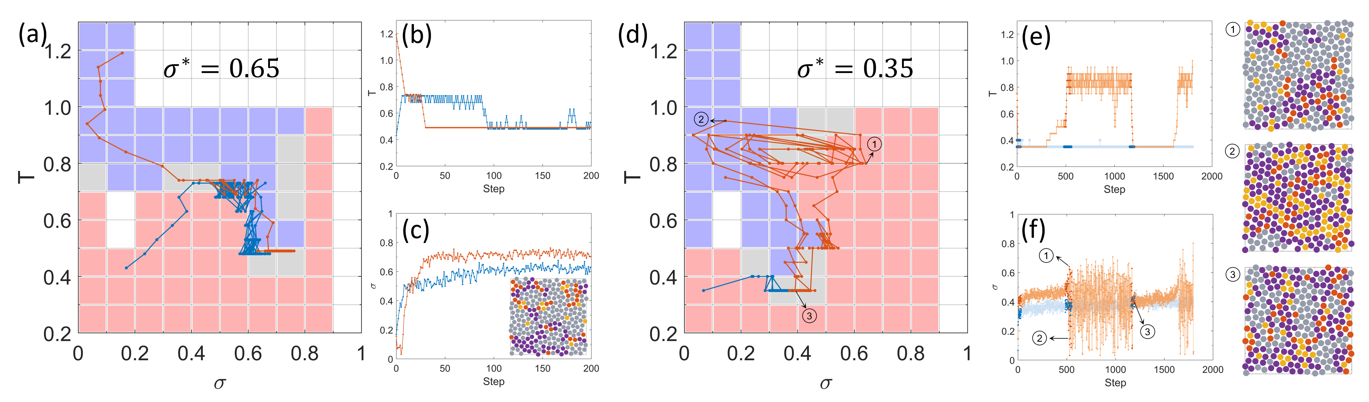
Fig.  10: [RL4] Reinforcement learning for other assemblies of patchy particles with the targets $\sigma*^{=}0.65$ and $\sigma=0.35$. (a-c) The policy with selected trajectories during the tests and the corresponding temperature and $\sigma$ of the tests for $\sigma^{*}=0.65$. The mean and standard deviation of $\sigma$ from 20 independent samples are 0.63 and 0.03, respectively. The snapshot at the last point of the blue trajectory is given. (e-f) The temperature schedule and $\sigma$ of selected trajectories during the tests when $\sigma^{*}=0.35$. Three snapshots of the orange trajectory are given. (d) The trajectories of the tests on the policy plane in which only part of the data (darker points) is used. The mean and standard deviation of $\sigma$ from 20 independent samples are 0.42 and 0.14.

In RL1 and RL2, we use the target $\sigma=0.91$ to obtain the DDQC structure. This structure is an equilibrium one under a certain temperature. In this section, we show the proposed RL works also for the unknown target structures, which are not equilibrium state. To do this, we perform RL for different targets: $\sigma^{*}=0.65$ and $\sigma^{*}=0.35$ in patchy particle systems. The estimation of the policy is conducted by the Value Iteration method (Appendix A) instead of training the Q-table through numerous episodes because of the availability of sufficient data (see Table S1 in S.I.). As shown in Fig. 10, RL estimates different policies for different targets. For $\sigma^{*}=0.65$, the structure obtained from the estimated policy is close to DDQC but with many defects. The policy in Fig. 10(a) shows a border at the critical temperature at $T=0.7$. When $\sigma$ is small, the policy is similar to the case of [RL1] in Fig. 4-5, and it suggests to drive the temperature to $T^{*}$ so that $\sigma$ increases, that is to decrease $T$ if $T_{0}$ is high (orange trajectory) and to increase $T$ if $T_{0}$ is low (blue trajectory). Then, when $\sigma\gtrsim 0.6$, the policy suggests to decrease the temperature to make the motions of the particles slower. Figure 10 also shows how the policy prevents the DDQC state (in this case, the DDQC is the undesired structure as we set $s^{*}=0.65$) by increasing $T$ whenever $\sigma>0.8$.

In Fig. 10(d-f), the policy and tests for the target $\sigma^{*}=0.35$ are demonstrated. The policy can be divided into three regimes, represented by the snapshots 1, 2, and 3. At first, large $\sigma$ structure ($\sigma>0.5$) is avoided by increasing temperature (see snapshot 1 of Fig. 10(d-f)). When the temperature becomes $T\approx 0.85$, the structure strongly fluctuates with $0<\sigma<0.65$, for example, between snapshots 1 and 2. When $\sigma$ becomes small, the blue region in the policy around snapshot 2 suggests decreasing temperature, and the system attempts to reach a state such as snapshot 3. The structure near snapshot 3 is not stable, and after a long time, the structure changes. Then, a new cycle of snapshots $3\rightarrow 1\rightarrow 2$ occurs. The result reveals that RL can learn even when the target is unstable. The policy shows how we can obtain the target structure dynamically by changing the temperature.

4 Discussion and conclusion

We have investigated how RL learns and proposes policies for temperature control of patchy particles to form a DDQC. Our results suggest that the best policy for making DDQC is to change the temperature quickly to the critical temperature $T^{*}\approx 0.7$, keep the temperature until the system is dominated by the dodecagonal structures, and then decrease the temperature further to the final temperature to get the DDQC with fewer defects. It is noted that such critical temperature $T^{*}$ is autonomously found out by RL. At the critical temperature, the structural fluctuations are enhanced. As a result, there is more chance of getting the dodecagonal structure. At higher $T$, the particles are too mobile to make the ordered structures. On the other hand, at lower $T$, the particles are kinetically trapped in the metastable state, and it is unlikely to remove the defects. This temperature dependence is also seen in Fig. 6 in this work and Fig. 9 in Ref.⁷ about the formation of DDQC under the annealing (slow temperature change) and quenching (rapid temperature change). From the initial condition of random positions and orientations, the patchy particles cannot form DDQC by rapid quenching because the system gets trapped in the metastable state. On the other hand, during the annealing, the system has more chance to escape from the metastable states. In fact, as shown in Fig. 9 in Ref.⁷, the fluctuation of the structures is largest at $T\approx 0.75$, which is coincident with the critical temperature $T^{*}$ found from the estimated policy. In the estimated policy by RL, even when we start from low $T_{0}$, the policy suggests increasing temperature so that the system may escape from the metastable state. In ⁷, the DDQC can be generated by fixed annealing, which is sufficiently slow. However, this fixed temperature schedule is not efficient because it takes too much time to reach the critical temperature at which structural transition occurs. RL can learn that the critical temperature $T^{*}$ plays an important role in enhancing the probability of QC structural formation. We stress that our method feeds neither existence of the critical temperature nor its value. Our RL method automatically finds them during the training steps.

The choice of statistical quantities that characterise the structures is crucial for designing a successful RL system. This includes the choice of the relevant states and how finely to discretise the states (for Q-table). In the case of DDQC, the continuous state we choose is the ratio of the $\sigma$ particles because $\sigma$ can span over a wide range in $[0,1]$ under the investigated temperature. Therefore, the states can distinguish the DDQC from metastable and disordered structures. One can consider the $Z$ particles to evaluate the DDQC structure. However, under the same condition, the performance of Q-learning with $Z$ is not as good as Q-learning with $\sigma$ because the ratio of $Z$ spans over a narrower range. Methodologically, there is no limit of number of states in RL. For example, one may include two microscopic states, e.g. $\sigma$ and $Z$. When the dimension of states is much higher, the computational cost using Q-table is too high. Approximation of the Q-function by the small number of continuous basis functions is promising in this direction.

In this study, we use the states of $T$ and $\sigma$, the action space of change in temperature $\Delta T$, and the reward function of $(\sigma-\sigma^{*})^{2}$. However, we still need to consider many hyperparameters, such as the number of epochs $N_{\text{e}}$ during training and the effect of discretisation. We discuss some general issues: how prior knowledge can help reduce the calculation cost, the effect of discretisation of Q-table, and the effect of $\epsilon$-greedy, in Supplementary Information.

Q-learning RL in this study can be applied to various self-assembly systems. We demonstrate it for the system of patchy particles and isotropically interacting particles. Both systems show DDQC; nevertheless, the estimated policy of temperature control is qualitatively different. The results give us physical insights on the two systems. The system of patchy particles has metastable states, which have to be overcome to form DDQC, whereas the system of isotropically interacting particles is monostable.

We focus on the estimation of the policy for DDQC, which is stable at a certain range of temperature. However, our RL method is not limited to such a stable target structure. In fact, we demonstrate that RL can estimate temperature protocol for metastable and even transiently stable structures. In all cases, the critical temperature plays a significant role for the patchy particles. To obtain the metastable structure as a target, we may leave the system near the critical temperature at which structural fluctuation is large, and then, rapidly decrease the temperature so that the structure is frozen at the desired metastable state. When the target is not even at the metastable state, again we may wait at the critical temperature to obtain the structure at the target, and then, decrease the temperature. In this case, the structure is transient, and after some time, it escapes from the target structure. Still, we may increase the temperature at the critical temperature again so that the system returns to the structure. Those results, including the temperature protocol for DDQC, may be reached from sophisticated guess, but we think this is not the case for many people. We believe that RL, like any machine learning method, can assist our finding mechanisms of unknown phenomena and making decisions more efficiently. To tackle more complex, highly non-linear, and high dimensional problems, the combination of machine learning with expertise in decision making may help to understand the problem better.

There are many ways of doing reinforcement learning.^{32, 37} In their study on RL for self-assembly,³⁰ Whitelam and Tamblyn have shown that the evolutionary optimisation to train the neural network can learn actions on the control parameters, such as temperature and chemical potential, for the self-assembly of a target structure. Evolutionary optimisation takes a black-box approach to learn the action as a function of the state (or time), which is expressed by the weights in the neural network.³⁸ On the other hand, Q-learning relies on the maximisation of future reward, which is expressed by the Bellman’s equation. The sampling during training is also different in the two methods. The evolutionary optimisation requires the final outcome of the trajectory of the self-assembly process, while the Q-learning updates the policy iteratively by observing the state-action pair during the dynamical process. As a result, Q-learning works on-the-fly and requires less computational cost compared to evolutionary optimisation. We should stress that regardless of the differences, both evolution-type optimisation and Q-learning based on the Markov decision process estimate the policy that can produce the target faster than a conventional cooling scheme. More studies are necessary to clarify generic guidelines on how to choose a suitable RL model.

Although RL can estimate the best temperature protocol, it has to be related with the physical properties of the system. The work in Ref.¹⁵ proposed a temperature protocol based on free energy calculation of nucleation barrier and metastability of the free energy minima. Although it treated a toy model, relating the physical properties of QC formation and performance of RL would be an interesting future direction.

To summarise, we propose the method based on RL to estimate the best policy of temperature control for the self-assemblies of patchy particles to obtain the DDQC structures. From the estimated policy, we successfully obtain the DDQCs even for the system size larger than the size we use for training. The key to the success is that RL finds the critical temperature of the DDQC self-assembly during training. The estimated policy suggests that first, we change the temperature to the critical temperature so that the larger fluctuations enhance the probability of forming DDQC, and then decrease the temperature slightly to remove defects. The estimated policy is more efficient than the pre-fixed temperature schedule used in the previous studies and DDQC can be generated in a shorter time. The mechanism of learning optimal policy is demonstrated in the simple triple-well model. In order to avoid metastable states, the optimal policy suggests increasing the temperature if we start from a low temperature. The RL is capable of giving insights to different self-assembled systems, and dynamically adapting the policy in response to unstable target. We should stress that our method can be applied to other parameters that we may control. Therefore, we believe that the method presented in this work can be applied to other self-assembly problems.

Author Contributions

U.L. performed the simulations and analysed the data. N.Y. designed the research. All the authors developed the method and were involved in the evaluation of the data and the preparation of the manuscript.

Conflicts of interest

There are no conflicts to declare.

Data Availability

The codes of RL for self-assembly of patchy particles and RL for triple-well model can be found at https://github.com/ULieu/RL_patchy and https://github.com/ULieu/RL_3well.

Appendix A Appendix: Reinforcement Learning with Value Iteration method

Q-learning is a model-free method in RL. As shown in the main article, the Q-table is updated during training (BD simulations at given $T$) and eventually the policy is determined from the Q-table. Here we propose to use Value Iteration to utilise the data from training Q-table. Value Iteration is a model-based method, i.e. we need to know the model dynamics (transition probability of the next states given current states and actions).^{32, 37} Therefore, we first estimate the transition probability from the current state $s=(\sigma,T)$ to the next state $s^{\prime}$ under the action $a$, $P(\sigma^{\prime},T^{\prime}|\sigma,T,a)$, from empirical sampling obtained for the Q-learning in RL1. Then, we use Bellman’s equation to estimate the value function, from which we can estimate the policy of the temperature change. Here, we show how to calculate the value function

1. Sampling data $S(s,a,s^{\prime})$

2. Discretising the state spaces and calculating the transition probability $P(s^{\prime}|s,a)$

3. Performing value iteration on the discretised state space:

   • initialise the value function $V(s)=0$

   • in each iteration, calculate

     $$Q(s,a)=\sum_{s^{\prime}}P(s^{\prime}|s,a)[R(s,a,s^{\prime})+\gamma V(s^{\prime})];$$ (10)

and the value function in this iteration is $V(s)=\max_{a}Q(s,a)$.

For the self-assembly of patchy particles in our study, there are two states $s=(\sigma,T)$. We report the result after 100 iterations when the value function converges. Note that the calculation of $V(\sigma,T)$ and policy uses the information of $P(\sigma^{\prime},T^{\prime}|\sigma,T,a)$ and no extra simulation is needed. The hyperparameters such as the target $\sigma^{*}$, reward function, can also be varied. Once the value function converges, one can determine the corresponding Q-value $Q(\sigma,T,a)$ and the policy $\pi(a|\sigma,T)=\operatorname*{arg\,max}_{a}Q(\sigma,T,a)$. The reward function and discount factor $\gamma$ in value iteration are chosen identical to that in Q-learning.