Robustness for Spectral Clustering of General Graphs
under Local Differential Privacy

Abstract

Spectral clustering is a widely used algorithm to find clusters in networks. Several researchers have studied the stability of spectral clustering under local differential privacy with the additional assumption that the underlying networks are generated from the stochastic block model (SBM). However, we argue that this assumption is too restrictive since social networks do not originate from the SBM. Thus, we delve into an analysis for general graphs in this work. Our primary focus is the edge flipping method – a common technique for protecting local differential privacy. On a positive side, our findings suggest that even when the edges of an $n$-vertex graph satisfying some reasonable well-clustering assumptions are flipped with a probability of $O(\log n/n)$, the clustering outcomes are largely consistent. Empirical tests further corroborate these theoretical findings. Conversely, although clustering outcomes have been stable for dense and well-clustered graphs produced from the SBM, we show that in general, spectral clustering may yield highly erratic results on certain dense and well-clustered graphs when the flipping probability is $\omega(\log n/n)$. This indicates that the best privacy budget obtainable for general graphs is $\Theta(\log n)$.

1 Introduction

As the demand for trustworthy artificial intelligence grows, the need to protect user privacy becomes more crucial. Several methods have been proposed to address this concern. Among these, differential privacy is the most common one. Differential privacy [1] measures the amount of privacy a system leaks by using a metric called the privacy budget. This method involves corrupting users’ information, then processing the corrupted data to obtain statistical conclusions while still maintaining privacy. Developing algorithms that can accurately provide statistical conclusions from the corrupted information is a topic of interest among many researchers [2].

In this work, we are interested in a variant of differential privacy called local differential privacy [3]. Unlike traditional differential privacy, local differential privacy does not allow the collection of all users’ information before it is corrupted. Instead, it requires users to corrupt their data at their local devices before sending it to central servers. This ensures that users’ information is not leaked during transmission. Local differential privacy is used by companies [4, 5] for their services.

We focus on algorithms for social networks. In a social network, each user is represented by a node, and their relationships with other users are represented by edges. One technique for protecting user privacy under the local differential privacy notion is randomized response or edge flipping [6, 7, 8]. In this technique, before sending their adjacency vector (which represents their friend list) to the central server, each bit in the adjacency vector is flipped with a specified probability $p$. We obtain a local differential privacy with the budget of $\Theta(\log 1/p)$ by the flipping.

Several algorithms [9, 10] have been proposed for processing social networks of which edges are flipped. These include graph clustering algorithms such as [11, 12, 13]. One of the most widely used and scalable graph clustering algorithms – spectral clustering [14] – has also received a lot of attention in this context. Many analyses such as [15] have been recently done for the algorithms. However, all of these analyses assume that the input social networks are generated from the stochastic block models (SBM).

1.1 Our Contribution

We argue that assuming that the input graph is generated from the SBM is too restrictive. Thus, in this study, we consider the robustness of spectral clustering for general graphs. In what follows, let $G$ be an $n$-vertex input graph. Our main contribution of Section 3 can be summarized by the following theorem:

Theorem 1.1.

Let $G^{\prime}$ be obtained from $G$ via the edge flipping mechanism with probability $p=O(\log n/n)$. Then, under some reasonable assumptions, the number of vertices misclassified by the spectral clustering algorithm by running it on $G^{\prime}$ instead of $G$ is $O(\eta(G)\cdot n)$ with probability $1-o(1)$, where $\eta(G)$ is a small constant.

In simpler terms, we demonstrate that:

$$\begin{array}[]{cc}\text{Spectral clustering is robust against edge flipping or the randomized response}\\ \text{method with probability }p=O(\log n/n),\text{ or privacy budget }\epsilon=\Omega(\log n).\end{array}$$ (1.1)

One of the results of [12] proves (1.1), assuming that the input social networks are generated from the SBM. We make much weaker assumptions in our work. The only two assumptions we require are 1) the social network has a sufficient cluster structure and 2) its maximum degree is sufficiently large.

We use some ideas from the proof by Peng and Yoshida [16] who have studied the sensitivity of spectral clustering algorithms. However, their work focuses on scenarios where each edge is removed with a specific probability. In contrast, local differential privacy not only removes edges but also adds edges to social networks. Furthermore, the number of edges added is often much greater than those removed. Thus, we can only incorporate their concepts in limited sections of our proof, with the core components (like Section 3.3) being original.

The work detailed in [15] demonstrates that stable results from graphs produced by SBM are unattainable with a privacy budget of $o(\log n)$. This suggests that having such a privacy budget for general graphs is also implausible. Because it has been proven that a constant privacy budget can be achieved for dense, well-clustered graphs generated by SBM [15], one might anticipate a similar outcome for general graphs. Regrettably, in Section 4 of this paper, we present a dense, well-clustered graph where spectral clustering results significantly shift when edges are flipped at a probability of $\omega(\log n/n)$. This indicates that even within this regime, securing a smaller privacy budget is not feasible.

Remark 1.2.

For many readers, it may seem counter-intuitive that the privacy budget increases with the number of users, given that differential privacy tends to be more effective with larger databases. This can be explained by considering the nature of the data being protected. In relational databases or general graph differential privacy, there are $n$ pieces of information to protect. However, for local edge differential privacy, the protection extends to $O(n^{2})$ edge information.

Remark 1.3.

Spectral clustering analysis under local differential privacy is a relatively recent area of exploration. However, there is a substantial body of work on graph clustering with differential privacy, as evidenced by studies like [12, 17]. Notably, a recent study by [18] provides both upper and lower limits for privacy budgets pertaining to dense graphs generated from the SBM.

2 Preliminaries

2.1 Notation

Edge-subsets.

For the remainder of the paper, we assume that $G=(V,E(G))$ is a graph of $n$ vertices. For any subset $F\subseteq\binom{V}{2}$, we denote by $G\triangle F$ the graph $(V,E(G)\triangle F)$. By $F\sim_{p}\binom{V}{2}$, we mean a subset $F$ is taken uniformly from $\binom{V}{2}$ with probability $p$.

Cuts.

For a subset $S\subseteq V$ of vertices, we denote by $\mkern 1.5mu\overline{\mkern-1.5muS\mkern-1.5mu}\mkern 1.5mu$ the complement set $V\setminus S$. Further, given two subsets $A,B\subseteq V$ with $A\cap B=\varnothing$, let $e_{G}(A,B)$ denote the number of edges of $G$ with one endpoint in $A$ and one in $B$. For any two sets of nodes $S,S^{\prime}\subseteq V$, $d_{\text{size}}(S,S^{\prime})$ is given by

$$d_{\text{size}}(S,S^{\prime})=\min\left(|S\triangle S^{\prime}|+|\mkern 1.5mu\overline{\mkern-1.5muS\mkern-1.5mu}\mkern 1.5mu\triangle\mkern 1.5mu\overline{\mkern-1.5muS^{\prime}\mkern-1.5mu}\mkern 1.5mu|,|S\triangle\mkern 1.5mu\overline{\mkern-1.5muS^{\prime}\mkern-1.5mu}\mkern 1.5mu|+|\mkern 1.5mu\overline{\mkern-1.5muS\mkern-1.5mu}\mkern 1.5mu\triangle S^{\prime}|\right).$$

As $|S\triangle T|=|\mkern 1.5mu\overline{\mkern-1.5muS\mkern-1.5mu}\mkern 1.5mu\triangle\mkern 1.5mu\overline{\mkern-1.5muT\mkern-1.5mu}\mkern 1.5mu|$, we can equivalently write $d_{\text{size}}(S,S^{\prime})=2|S\triangle S^{\prime}|$. A cut $(S,\mkern 1.5mu\overline{\mkern-1.5muS\mkern-1.5mu}\mkern 1.5mu)$ is similar to $(S^{\prime},\mkern 1.5mu\overline{\mkern-1.5muS^{\prime}\mkern-1.5mu}\mkern 1.5mu)$ if $d_{\text{size}}(S,S^{\prime})$ is small.

Spectral Graph Theory.

Any $n\times n$ real symmetric matrix $A$ has $n$ real eigenvalues. We denote the $i$-th smallest eigenvalue of $A$ as $\lambda_{i}(A)$, i.e. $\lambda_{1}(A)\leq\lambda_{2}(A)\leq\cdots\leq\lambda_{n}(A)$. For any graph $G$, the Laplacian matrix $L_{G}$ is given by $D_{G}-A_{G}$, where $D_{G}$ is the diagonal degree matrix with $(D_{G})_{ii}=\deg_{G}(i)$ and $A_{G}$ is the adjacency matrix of $G$.

In this work, we define the spectral robustness of the graph $G$ as $\eta(G):=\frac{\Delta(G)\lambda_{2}(L_{G})}{\lambda_{3}(L_{G})^{2}}$, where $\Delta(G)$ denotes the maximum degree of any vertex of $G$.

2.2 Edge Differential Privacy under Randomized Response

The concept of $\epsilon$-edge differential privacy is defined as follows.

Definition 2.1 ($\epsilon$-edge differential privacy [19]).

Let $G$ be a social network and let $Y$ be a randomized mechanism that outputs $Y(G)$ from the social network $G$. For any $\epsilon>0$, any possible output of the mechanism $Y$ denoted by $y$, and any two social networks $G^{(1)}=(V,E^{(1)}(G))$ and $G^{(2)}=(V,E^{(2)}(G))$ that differ by one edge, we say that $Y$ is $\epsilon$-edge differentially private if $e^{-\epsilon}\leq\frac{\Pr[Y(G^{(1)})=y]}{\Pr[Y(G^{(2)})=y]}\leq e^{\epsilon}.$

Intuitively, a lower value of $\epsilon$ results in better privacy protection. In this research, for $0\leq p\leq 0.5$, we investigate a randomized mechanism $Y_{p}$ that seeks to generate a result highly similar to spectral clustering outcomes, using randomized response. The mechanism $Y_{p}$ is defined as $Y_{p}=\mathcal{SC}\circ\mathcal{F}_{p}$, where $\mathcal{F}_{p}$ represents a randomized function that modifies the relationship between each node pair with a probability of $p$, and $\mathcal{SC}$ is a function for computing spectral clustering. In other words, the randomized mechanism performs spectral clustering on $G\Delta F$, in which $(u,v)\in F$ with a probability of $p$ for every $u,v\in V$. The following theorem is shown in [8].

Theorem 2.1 ([8]).

The publication $Y_{p}$ is $\epsilon$-edge differential privacy if $\frac{1-p}{p}\leq e^{\epsilon}$.

The previous theorem implies that $Y_{p}$ is $\epsilon$-edge differential private for $\epsilon\geq\ln(1-p)-\ln p$. When $p$ is small, we have that $\ln(1-p)\approx 0$ and the privacy budget of the publication $Y_{p}$ is $\Omega(\log 1/p)$.

2.3 Spectral Clustering

For a graph $G$, the general goal of clustering techniques is to find a good cut $(S,\mkern 1.5mu\overline{\mkern-1.5muS\mkern-1.5mu}\mkern 1.5mu)$ such that $e_{G}(S,\mkern 1.5mu\overline{\mkern-1.5muS\mkern-1.5mu}\mkern 1.5mu)$ is small, and most of the edges of $G$ are either concentrated in $S$ or $\mkern 1.5mu\overline{\mkern-1.5muS\mkern-1.5mu}\mkern 1.5mu$. In order to avoid trivial cuts (for example where $S$ comprises of a single vertex), it is customary to instead define the cut-ratio $\alpha_{G}(S)=\frac{e_{G}(S,\mkern 1.5mu\overline{\mkern-1.5muS\mkern-1.5mu}\mkern 1.5mu)}{|S||\mkern 1.5mu\overline{\mkern-1.5muS\mkern-1.5mu}\mkern 1.5mu|}$ and find cuts that minimize $\alpha_{G}(S)$ [20, 21]. $\alpha(G)=\min\limits_{\varnothing\subsetneq S\subsetneq V}\alpha_{G}(S)$ is defined as the cut-ratio of $G$. Unless otherwise specified, we shall denote by $S^{\ast}$ the cut that achieves $\alpha_{G}(S^{\ast})=\alpha(G)$.

Another widely used way of defining the cut-ratio is $\alpha^{\prime}_{G}(S)=\frac{e_{G}(S,\mkern 1.5mu\overline{\mkern-1.5muS\mkern-1.5mu}\mkern 1.5mu)}{\min(|S|,|\mkern 1.5mu\overline{\mkern-1.5muS\mkern-1.5mu}\mkern 1.5mu|)}$ [16, 22, 23]. We observe that these two definitions are related:

Lemma 2.2.

$\frac{1}{2}\cdot n\alpha_{G}(S)\leq\alpha^{\prime}_{G}(S)\leq n\alpha_{G}(S)$.

Proof.

Observe that $\frac{n}{2}\cdot\alpha_{G}(S)=\frac{|S|+|\mkern 1.5mu\overline{\mkern-1.5muS\mkern-1.5mu}\mkern 1.5mu|}{2}\cdot\frac{e_{G}(S,\mkern 1.5mu\overline{\mkern-1.5muS\mkern-1.5mu}\mkern 1.5mu)}{|S||\mkern 1.5mu\overline{\mkern-1.5muS\mkern-1.5mu}\mkern 1.5mu|}=\frac{1}{2}\left(\frac{e_{G}(S,\mkern 1.5mu\overline{\mkern-1.5muS\mkern-1.5mu}\mkern 1.5mu)}{|S|}+\frac{e_{G}(S,\mkern 1.5mu\overline{\mkern-1.5muS\mkern-1.5mu}\mkern 1.5mu)}{|\mkern 1.5mu\overline{\mkern-1.5muS\mkern-1.5mu}\mkern 1.5mu|}\right)\leq\alpha^{\prime}_{G}(S)$, and $\alpha^{\prime}_{G}(S)=\alpha_{G}(S)\cdot\max(|S|,|\mkern 1.5mu\overline{\mkern-1.5muS\mkern-1.5mu}\mkern 1.5mu|)\leq n\cdot\alpha_{G}(S)$. ∎

Lemma 2.2 will be useful in converting results formulated using $\alpha^{\prime}_{G}$ to those using our cut-ratio $\alpha_{G}$.

Spectral clustering uses the eigenvalues and eigenvectors of $L_{G}$ to compute a cut of $S$. Let us denote by $\mathcal{SC}_{2}$ the following algorithm:

• Compute (or approximate) the second smallest eigenvector $\vec{v}=(v_{1},\dots,v_{n})^{\intercal}$ of $L_{G}$, and reorder the vertices of $G$ such that $v_{1}\leq\cdots\leq v_{n}$.

• Return the cut $(S,\mkern 1.5mu\overline{\mkern-1.5muS\mkern-1.5mu}\mkern 1.5mu)$, where $S=\{v_{1},\ldots,v_{i_{0}}\}$ and $i_{0}=\mathop{\text{argmin}}\limits_{1\leq i\leq n}\alpha_{G}(v_{1},\ldots,v_{i})$.

The cut-ratio of $G$ can be quantified very precisely via the famous Cheeger’s inequality.

Lemma 2.3 (Cheeger’s Inequality[24, 25]).

$\lambda_{2}(L_{G})\leq n\alpha(G)\leq\sqrt{8\Delta(G)\lambda_{2}(L_{G})}.$

We shall also use the following improvement of Lemma 2.3:

Lemma 2.4 (Improved Cheeger Inequality[23]).

Let $\mathcal{SC}_{2}(G)$ denote the cut given by the spectral clustering algorithm. Then,

$$\alpha_{G}(\mathcal{SC}_{2}(G))\leq O\left(\frac{\lambda_{2}(L_{G}){\Delta(G)}^{1/2}}{n{\lambda_{3}(L_{G})}^{1/2}}\right).$$

Lemma 2.3 and 2.4 give us a way of quantifying the quality of the cut output by $\mathcal{SC}_{2}$ in terms of the cut-ratio of $G$. Indeed,

$$\alpha_{G}(\mathcal{SC}_{2}(G))\leq O\left(\frac{{\Delta(G)}^{1/2}}{{\lambda_{3}(L_{G})}^{1/2}}\right)\cdot\alpha(G).$$ (2.1)

Let $S^{\ast}$ be the cut of $G$ with the smallest cut-ratio. While equation (2.1) can be interpreted as a measure of how close $\mathcal{SC}_{2}(G)$ is with $S^{\ast}$, we shall need stability results from [16, 23] to precisely bound $d_{\text{size}}(\mathcal{SC}_{2}(G),S^{\ast})$.

Lemma 2.5 (Stability of min-cut).

Let $G=(V,E)$ be any graph with optimal min-cut $S^{\ast}$. Then, for any $\rho\geq 1$, if $S\subseteq V$ satisfies $\alpha_{G}(S)\leq\rho\cdot\alpha_{G}(S^{\ast})$, then

$$d_{\text{size}}(S,S^{\ast})\leq O\left(\frac{\lambda_{2}(L_{G})\Delta(G)^{1/2}}{\lambda_{3}(L_{G})^{3/2}}\cdot\rho\right)\cdot n.$$

Proof (sketch)..

Observe that by Lemma 2.2, $\alpha_{G}(S)\leq\rho\cdot\alpha_{G}(S^{\ast})$ implies $\alpha^{\prime}_{G}(S)\leq 2\rho\cdot\alpha^{\prime}_{G}(S^{\ast})$. This lemma then follows from a direct application of Lemma 3.5 of [16]. ∎

2.4 Concentration Inequalities

We also require some concentration inequalities for random variables, which we present here.

Lemma 2.6 (Hoeffding’s inequality [26]).

Let $X_{1},\ldots,X_{n}$ be independent random variables such that $a_{i}\leq X_{i}\leq b_{i}$ almost surely. If $S=X_{1}+\cdots+X_{n}$, then we have

$$\Pr\left[S\leq{\mathbb{E}}(S)-t\right]\leq\exp\left(-\frac{2t^{2}}{\sum_{i=1}^{n}(b_{i}-a_{i})^{2}}\right).$$

Lemma 2.7 (Chernoff bound for binomial random variables [27]).

For a binomial random variable $X$ with mean $\mu$ and $t>0$, we have

$$\Pr\left[X\geq\mu+t\right]\leq\exp\left(-\frac{t^{2}}{2\mu+t}\right).$$

Lemma 2.8 (Weyl’s Inequality [28]).

For any real symmetric matrices $M$ and $H$

$$|\lambda_{i}(M+H)-\lambda_{i}(M)|\leq\|H\|_{2},$$

Where $\|H\|_{2}$ denotes the spectral norm of $H$.

2.5 Assumptions

In order to demonstrate the robustness of spectral clustering, we require assumptions on the social network $G$ and the probability $p$ of edge flipping. Recall that $F\sim_{p}\binom{V}{2}$ is the set of vertex pairs to be flipped.

Assumption 2.9.

We assume the following:

1.	$p<\log n/10n$,
2.	(a) $\Delta(G)\geq 10\log n\lambda_{3}(L_{G})$,	(b) $\lambda_{2}(L_{G})\geq 1/10$,	(c) $\eta(G):=\frac{\lambda_{2}(L_{G})\Delta(G)}{\lambda_{3}(L_{G})^{2}}$ is small,
	(d) $\lambda_{3}(L_{G})\geq 10\log n$,
3.	Let the minimum cuts of $G$ and $G\triangle F$ be $(S^{\ast},\mkern 1.5mu\overline{\mkern-1.5muS^{\ast}\mkern-1.5mu}\mkern 1.5mu)$ and $(S^{\ast}_{F},\mkern 1.5mu\overline{\mkern-1.5muS^{\ast}_{F}\mkern-1.5mu}\mkern 1.5mu)$, respectively. Then each of $|S^{\ast}|,|\mkern 1.5mu\overline{\mkern-1.5muS^{\ast}\mkern-1.5mu}\mkern 1.5mu|,|S^{\ast}_{F}|,|\mkern 1.5mu\overline{\mkern-1.5muS^{\ast}_{F}\mkern-1.5mu}\mkern 1.5mu|$ have size at least $n/10$.

Plausibility of Assumption 2.9:

1. The first assumption can be justified by our discussion in Section 2.2, where we observe that privacy can be maintained as long as $p$ is $\Omega(1/n)$. We further note that, if $G$ is a sparse social network with $O(n)$ edges and $p\gg\log n/n$, then as ${\mathbb{E}}(|F|)=\Omega(n\log n)$, $G\triangle F$ will have too much noise, and would become close to the Erdős-Rényi random graph $F\sim\mathcal{G}(n,p)$. Spectral algorithms cannot perform well for these graphs. For example, it is shown in [29] that the eigenvalues of the normalized Laplacian $\mathcal{L}_{F}$ are close to those of the expected values. A quick calculation shows that the second and third eigenvalues of ${\mathbb{E}}(\mathcal{L}_{F})$ are both equal (and close to $1$), implying the inefficiency of spectral clustering algorithms on $\mathcal{G}(n,p)$ for $p$ asymptotically larger than $\log n/n$.

   On the other hand, one may think that values of $p$ larger than $\log n/n$, for example $p=\Omega(1)$ is achievable by the edge flipping mechanism if the input graph $G$ is dense. However, there are two issues with this: firstly, social networks are not dense in practice. Secondly, we demonstrate in Section 4, a well-clustered dense graph, whose sparsest cut changes drastically when introducing noise $p=\omega(\log n/n)$.

2. The second assumption derives from usual properties of social networks. Recall that we have the following chain of inequalities on the eigenvalues of $L_{G}$:

   $$0=\lambda_{1}(L_{G})\leq\lambda_{2}(L_{G})\leq\cdots\leq\lambda_{n}(L_{G})<2\Delta(G).$$

   This assumption asserts that there are big gaps between $\lambda_{2}(L_{G})$, $\lambda_{3}(L_{G})$ and $\Delta(G)$. First, we note that most social networks that we encounter in practice, have super-nodes (nodes of degree $\Omega(n)$), justifying our assumption (a). Further, (b) ensures that $G$ is well-connected: note that disconnected graphs have $\lambda_{2}(L_{G})=0$ and graphs that have small edge-separators have a small $\lambda_{2}(L_{G})$. Finally, (c) ensures that there is a gap between $\lambda_{3}(L_{G})$ and $\lambda_{2}(L_{G})$, which ensures that the graph has a good bi-cluster structure, which lets $\mathcal{SC}_{2}$ find good clusters in $G$.

   Observe that using inequalities (a), (b) and (c), we can deduce that $\lambda_{3}(L_{G})=\frac{\lambda_{2}(L_{G})\Delta(G)}{\lambda_{3}(L_{G})\eta(G)}\geq\frac{\log n}{\eta(G)}$, which implies our assumption of (d).

3. Our final assumption stems from the fact that usually social networks admit linearly sized clusters, and also we are usually interested in detecting clusters of larger size via the definition of the cut ratio $\alpha(G)$, for example.

3 Main Theorem

We restate and prove a formal version of Theorem 1.1 in this section.

Theorem 3.1.

Let $G=(V,E)$ be a graph and $p$ satisfy Assumption 2.9. Let $F\sim_{p}\binom{V}{2}$. Then, with probability at least $1-5n^{-8/5}$,

$$d_{\text{size}}\left(\mathcal{SC}_{2}(G),\mathcal{SC}_{2}(G\triangle F)\right)=O(\eta(G)\cdot n).$$

Proof Structure..

Suppose $S^{\ast}$ and $S_{F}^{\ast}$ are the optimum min-cuts of $G$ and $G\triangle F$. Denote by $S$ and $S_{F}$ the outputs of $\mathcal{SC}_{2}$ on $G$ and $G\triangle F$, respectively.

The key idea is to bound $d_{\text{size}}(S,S_{F})$ using triangle inequality:

$$d_{\text{size}}(S,S_{F})\leq d_{\text{size}}(S,S^{\ast})+d_{\text{size}}(S^{\ast},S^{\ast}_{F})+d_{\text{size}}(S^{\ast}_{F},S_{F}).$$ (3.1)

We bound each of the terms in their own subsection below. Observe that by Equations (3.2), (3.6) and (3.9), we obtain

$$d_{\text{size}}(S,S_{F})\leq O\left(\frac{\lambda_{2}(L_{G})\Delta(G)}{\lambda_{3}(L_{G})^{2}}\right)\cdot n=O(\eta(G)\cdot n)$$

with probability at least $1-4n^{-21/11}-n^{-8/5}\geq 1-5n^{-8/5}$, completing the proof. ∎

In the remainder of this section, we bound each term appearing in the right side of Equation (3.1).

3.1 The term $d_{\text{size}}(S,S^{\ast})$.

An upper bound on this term is a direct corollary of Cheeger’s inequality and stability: observe that Lemma 2.5 and (2.1) give us

$$d_{\text{size}}(S,S^{\ast})\leq O\left(\frac{\lambda_{2}(L_{G})\Delta(G)^{1/2}}{\lambda_{3}(L_{G})^{3/2}}\cdot\frac{\Delta(G)^{1/2}}{\lambda_{3}(L_{G})^{1/2}}\right)\cdot\ n=O\left(\frac{\lambda_{2}(L_{G})\Delta(G)}{\lambda_{3}(L_{G})^{2}}\right)\cdot n$$ (3.2)

3.2 The term $d_{\text{size}}(S^{\ast}_{F},S_{F})$.

First, we describe a lemma to compare the eigenvalues and maximum degrees of $G\triangle F$ and $G$.

Lemma 3.2.

Let $G$ have $n$ vertices, and $F\sim\mathcal{G}(n,p)$. Under Assumption 2.9, with probability at least $1-3n^{-21/11}$, all of the following hold:

(a) $\lambda_{2}(L_{G\triangle F})\leq\lambda_{2}(L_{G})$,

(b) $\lambda_{3}(L_{G\triangle F})\geq\lambda_{3}(L_{G})/10$,

(c) $\Delta(G\triangle F)\leq 2\Delta(G)$.

Proof.

Part (a). By monotonicity of $\lambda_{2}$, $\lambda_{2}(L_{G\triangle F})\leq\lambda_{2}(L_{G\cup F})$. As $\lambda_{2}(L_{G\cup F})\leq\lambda_{2}(L_{G})+\lambda_{2}(L_{F\setminus G})$, and $p<\log n/10n$, $F$ (and hence $F\setminus G$) is almost surely disconnected [30], implying $\lambda_{2}(L_{F\setminus G})=0$. Hence, we have $\lambda_{2}(L_{G\triangle F})\leq\lambda_{2}(L_{G\cup F})\leq\lambda_{2}(L_{G})$. $\blacksquare$

Part (b). For this part, we shall use Weyl’s Inequality as follows: suppose $F_{1}=F\setminus G$ and $F_{2}=G\cap F$ be subgraphs of $F$ on the vertex set $V(G)$. By additivity of the Laplacian, $L_{G\triangle F}-L_{G}=L_{F_{1}}-L_{F_{2}}$. Now as $\|A\|_{2}=\max_{x\in\mathbb{R}^{n}}x^{\intercal}Ax$ for any symmetric $n\times n$ matrix $A$, which implies

$$\|L_{G\triangle F}-L_{G}\|_{2} =\max_{x\in\mathbb{R}^{n}}\left|x^{\intercal}L_{F_{1}}x-x^{\intercal}L_{F_{2}}x\right|\leq\max_{x\in\mathbb{R}^{n}}x^{\intercal}L_{F}x=\lambda_{n}(L_{F})\leq 2\Delta(F).$$

By the union bound, note that for any $v\in V(G)$,

$$\Pr[\Delta(F)>\frac{9}{2}\log n]\leq n\cdot\Pr[\deg_{F}(v)>\frac{9}{2}\log n]\leq n\cdot\Pr\left[\deg_{F}(v)-p(n-1)>4\log n\right].$$ (3.3)

Using the Chernoff bound, the probability in (3.3) is at most

$$n\cdot\exp\left(-\frac{16(\log n)^{2}}{2(n-1)p+4\log n}\right)<n\cdot\exp\left(-\frac{16(\log n)^{2}}{\frac{11}{2}\log n}\right)=n\cdot\exp\left(-\frac{32}{11}\log n\right)=n^{-21/11},$$ (3.4)

Thus $\|L_{G\triangle F}-L_{G}\|_{2}\leq 9\log n$ holds with probability at least $1-n^{-21/11}$. By Weyl’s inequality and Assumption 2.9(2),

$$\lambda_{3}(L_{G})-\lambda_{3}(L_{G\triangle F})\leq 9\log n\leq\frac{9}{10}\lambda_{3}(L_{G}),$$

finishing the proof of (b). $\blacksquare$

Part (c). Observe that for every vertex $v\in V(G)$, we have

$$\deg_{G\triangle F}(v)-\deg_{G}(v)\leq\deg_{F}(v)\leq\Delta(F).$$

Hence,

$$\Pr\left[\deg_{G\triangle F}(v)>\deg_{G}(v)+\Delta(G)\right]\leq\Pr\left[\Delta(F)>\Delta(G)\right]\leq\Pr\left[\Delta(F)>10\log n\right].$$

By a similar calculation to (3.3) and (3.4), we conclude that $\deg_{G\triangle F}(v)>\deg_{G}(v)+\Delta(G)$ holds with probability at most $n^{-4}$. Again, by the union bound, with probability at least $1-n^{-3}$, we have

$$\deg_{G\triangle F}(v)\leq\deg_{G}(v)+\Delta(G)\mbox{ for all }v\in V(G).$$ (3.5)

Taking the maximum of (3.5) over all $v$, we see that (c) holds with probability at least $1-n^{-3}$, which is greater than $1-n^{-21/11}$. $\blacksquare$

As the assertions of (a), (b), (c) each hold with probability at least $1-n^{-21/11}$, all of them simultaneously hold with probability at least $1-3n^{-21/11}$, completing our proof of Lemma 3.2. ∎

Now, observe that by the same argument as (3.2) in addition with Lemma 3.2, we get that with probability at least $1-3n^{-21/11}$,

$$d_{\text{size}}(S^{\ast}_{F},S_{F})\leq O\left(\frac{\lambda_{2}(L_{G\triangle F})\Delta(G\triangle F)}{\lambda_{3}(L_{G\triangle F})^{2}}\right)\cdot n=O\left(\frac{\lambda_{2}(L_{G})\Delta(G)}{\lambda_{3}(L_{G})^{2}}\right)\cdot n$$ (3.6)

3.3 The term $d_{\text{size}}(S^{\ast},S^{\ast}_{F})$.

For the remainder of this section, let $\gamma_{0}$ be given by

$$\gamma_{0}:=200\sqrt{{\Delta(G)}/{\lambda_{3}(L_{G})}}>200\sqrt{10\log n}.$$

In order to bound $d_{\text{size}}(S^{\ast},S^{\ast}_{F})$, we require the following rather technical lemma.

Lemma 3.3.

Let $S^{*}$ denote the minimum cut of $G$ and $S^{*}_{F}$ denote the minimum cut of $G\triangle F$. Suppose $n/2\geq|S^{*}|,|S^{*}_{F}|\geq\epsilon n$ for some $1/2>\epsilon>0$. Further, suppose $\alpha_{G}(S^{*}_{F})\geq\gamma_{0}\alpha_{G}(S^{*})$. Then,

$$\Pr\left(\gamma_{0}\alpha_{G\triangle F}(S^{\ast}_{F})-\alpha_{G\triangle F}(S^{\ast})<0\right)<\exp\left(-\frac{4\left(\gamma_{0}^{2}-1\right)^{2}}{25\gamma_{0}^{2}}\cdot\alpha_{G}(S^{\ast})^{2}\epsilon^{2}n^{2}\right).$$ (3.7)

As the proof is involved, we defer it to the end of this section.

First, we demonstrate the bound on $d_{\text{size}}(S^{\ast},S^{\ast}_{F})$ using Lemma 3.3. We consider two cases:

• Case 1. $\alpha_{G}(S^{\ast}_{F})\leq\gamma_{0}\alpha_{G}(S^{\ast})$: In this case, Lemma 2.5 directly gives us

  $$d_{\text{size}}(S^{\ast},S^{\ast}_{F})\leq O\left(\frac{\gamma_{0}\lambda_{2}(L_{G})\Delta(G)^{1/2}}{\lambda_{3}(L_{G})^{3/2}}\right)\cdot n=O\left(\frac{\lambda_{2}(L_{G})\Delta(G)}{\lambda_{3}(L_{G})^{2}}\right)\cdot n.$$

• Case 2. $\alpha_{G}(S^{\ast}_{F})>\gamma_{0}\alpha_{G}(S^{\ast})$: In this case, setting $\epsilon=1/10$ in Lemma 3.3, we note that the probability that $\alpha_{G\triangle F}(S^{\ast})>\gamma_{0}\alpha_{G\triangle F}(S^{\ast}_{F})$ is at most:

  $$\exp\left(-\frac{(2\gamma_{0}^{2}-2)^{2}\alpha_{G}(S^{\ast})^{2}n^{2}}{2500\gamma_{0}^{2}}\right)< \exp\left(-\frac{\gamma_{0}^{2}}{2500}\cdot(\alpha_{G}(S^{\ast})\cdot n)^{2}\right)$$

  $$\ \ \ \stackrel{{\scriptstyle\text{Cheeger}}}{{<}} \exp\left(-{160\log n}\cdot\lambda_{2}(L_{G})^{2}\right)$$

  $$<\ \ \ \exp\left(-160\log n\cdot\frac{1}{100}\right)$$

  $$=\ \ \ n^{-8/5}$$

  The last line follows from Assumption 2.9(2). Hence, with probability at least $1-n^{-8/5}$, $\alpha_{G\triangle F}(S^{\ast})\leq\gamma_{0}\alpha_{G\triangle F}(S^{\ast}_{F})$ holds. By Lemma 2.5, this implies

  $$d_{\text{size}}(S^{\ast},S^{\ast}_{F})\leq O\left(\frac{\gamma_{0}\lambda_{2}(L_{G\triangle F})\Delta(G\triangle F)^{1/2}}{\lambda_{3}(L_{G\triangle F})^{3/2}}\right)\cdot n.$$

  Together with Lemma 3.2, we obtain that with probability at least $1-n^{-8/5}-3n^{-21/11}$,

  $$d_{\text{size}}(S^{\ast},S^{\ast}_{F}) \leq O\left(\frac{\Delta(G)^{1/2}}{\lambda_{3}(L_{G})^{1/2}}\cdot\frac{\lambda_{2}(L_{G\triangle F})\Delta(G\triangle F)^{1/2}}{\lambda_{3}(L_{G\triangle F})^{3/2}}\right)\cdot n$$ (3.8)

  $$=O\left(\frac{\lambda_{2}(L_{G})\Delta(G)}{\lambda_{3}(L_{G})^{2}}\right)\cdot n,$$ (3.9)

  finishing our upper bound on $d_{\text{size}}(S^{\ast},S^{\ast}_{F})$. $\blacksquare$

We now present our proof of Lemma 3.3.

Proof of Lemma 3.3..

The main idea behind the proof is as follows: first, we show that Lemma 3.3 holds with $S^{\ast}_{F}$ replaced with any fixed subset $A$. Then, we use the fact that

$$\Pr\left(\gamma_{0}\alpha_{G\triangle F}(S^{*}_{F})<\alpha_{G\Delta F}(S^{*})\right)$$ (3.10)

$$=\Pr\left(\gamma_{0}\alpha_{G\triangle F}(S^{*}_{F})<\alpha_{G\triangle F}(S^{*})\ |\ \alpha_{G}(S^{\ast}_{F})>\gamma_{0}\alpha_{G}(S^{\ast})\right)$$

$$=\sum\limits_{A:\alpha_{G}(A)>\gamma_{0}\alpha_{G}(S^{\ast})}\Pr(S^{*}_{F}=A)\cdot\Pr\left(\gamma_{0}\alpha_{G\triangle F}(S^{\ast}_{F})<\alpha_{G\triangle F}(S^{*})\ |\ S^{*}_{F}=A\right)$$

$$\leq\max\limits_{A:\alpha_{G}(A)>\gamma_{0}\alpha_{G}(S^{\ast})}\Pr\left(\gamma_{0}\alpha_{G\triangle F}(A)<\alpha_{G\triangle F}(S^{*})\right),$$

as $\sum_{A}\Pr(S^{\ast}_{F}=A)=1$.

Now, we bound $\Pr\left(\gamma_{0}\alpha_{G\triangle F}(A)<\alpha_{G\triangle F}(S^{*})\right)$ for any fixed $A$.

Claim 3.4.

Let $S^{\ast}$ denote the minimum cut of $G$. Suppose $\frac{n}{2}\geq|S^{\ast}|\geq\epsilon n$ for some $\frac{1}{2}>\epsilon>0$. Then, for any $\gamma>1$ and $\frac{n}{2}\geq|A|\geq\epsilon n$,

$$\Pr\left(\gamma\alpha_{G\triangle F}(A)-\alpha_{G\triangle F}(S^{\ast})<0\right)<\exp\left(-\frac{4\left(\gamma\alpha_{G}(A)-\alpha_{G}(S^{\ast})\right)^{2}}{25\gamma^{2}}\cdot\epsilon^{2}n^{2}\right).$$ (3.11)

Proof of Claim 3.4. Let $Y_{A}:=\gamma\alpha_{G\triangle F}(A)-\alpha_{G\triangle F}(S^{\ast})$. We wish to show that $Y_{A}\geq 0$ with high probability.

For any tuple $(x,y)\in V\times V$, define $X_{(x,y)}$ as the boolean random variable

$$X_{(x,y)}=\left\{\begin{array}[]{rl}1,&\mbox{if }xy\in E(G\triangle F),\\ 0,&\mbox{otherwise}.\end{array}\right.$$

As $X_{(x,y)}=X_{(y,x)}$, we abuse notation and write $X_{xy}$ as a shorthand for both these variables. Note that $X_{xy}$ are all mutually independent, and

$${\mathbb{E}}(X_{(x,y)})=\Pr(xy\in E(G\triangle F))=\left\{\begin{array}[]{cl}p,&\mbox{if }e\not\in E(G),\\ 1-p,&\mbox{if }e\in E(G).\end{array}\right.$$ (3.12)

Further, for any subset $A\subseteq V$, by definition

$$\alpha_{G\triangle F}(A)=\frac{e_{G\triangle F}(A,\mkern 1.5mu\overline{\mkern-1.5muA\mkern-1.5mu}\mkern 1.5mu)}{|A||\mkern 1.5mu\overline{\mkern-1.5muA\mkern-1.5mu}\mkern 1.5mu|}=\frac{1}{|A||\mkern 1.5mu\overline{\mkern-1.5muA\mkern-1.5mu}\mkern 1.5mu|}\cdot\sum_{(x,y)\in A\times\mkern 1.5mu\overline{\mkern-1.5muA\mkern-1.5mu}\mkern 1.5mu}X_{(x,y)},$$

Which, by (3.12), implies

$${\mathbb{E}}(\alpha_{G\triangle F}(A)) =\frac{1}{|A||\mkern 1.5mu\overline{\mkern-1.5muA\mkern-1.5mu}\mkern 1.5mu|}\cdot\left(\sum\limits_{e\in E_{G}(A,\mkern 1.5mu\overline{\mkern-1.5muA\mkern-1.5mu}\mkern 1.5mu)}{\mathbb{E}}(X_{e})+\sum\limits_{e\in A\times\mkern 1.5mu\overline{\mkern-1.5muA\mkern-1.5mu}\mkern 1.5mu\setminus E_{G}(A,\mkern 1.5mu\overline{\mkern-1.5muA\mkern-1.5mu}\mkern 1.5mu)}{\mathbb{E}}(X_{e})\right)$$ (3.13)

$$=\frac{1}{|A||\mkern 1.5mu\overline{\mkern-1.5muA\mkern-1.5mu}\mkern 1.5mu|}\cdot\left(e_{G}(A,\mkern 1.5mu\overline{\mkern-1.5muA\mkern-1.5mu}\mkern 1.5mu)\cdot(1-p)+|A||\mkern 1.5mu\overline{\mkern-1.5muA\mkern-1.5mu}\mkern 1.5mu|\cdot p-e_{G}(A,\mkern 1.5mu\overline{\mkern-1.5muA\mkern-1.5mu}\mkern 1.5mu)\cdot p\right)$$

$$=\frac{1}{|A||\mkern 1.5mu\overline{\mkern-1.5muA\mkern-1.5mu}\mkern 1.5mu|}\cdot\left(e_{G}(A,\mkern 1.5mu\overline{\mkern-1.5muA\mkern-1.5mu}\mkern 1.5mu)\cdot(1-2p)+|A||\mkern 1.5mu\overline{\mkern-1.5muA\mkern-1.5mu}\mkern 1.5mu|\cdot p\right)$$

$$=(1-2p)\cdot\alpha_{G}(A)+p.$$

Let $\mu$ denote the expectation of $Y_{A}$. By linearity and (3.13),

$$\mu={\mathbb{E}}(Y_{A}) =(1-2p)\cdot\left(\gamma\alpha_{G}(A)-\alpha_{G}(S^{\ast})\right)+p\cdot(\gamma-1)$$ (3.14)

$$>\frac{4}{5}\cdot\left(\gamma\alpha_{G}(A)-\alpha_{G}(S^{\ast})\right),$$

As $\gamma>1$ and $p<1/10$. We also have $\mu>0$, and $\Pr(Y_{A}<0)=\Pr(Y_{A}-\mu<-\mu).$ Now we shall use Hoeffding’s inequality to provide an upper bound on $\Pr(Y_{A}<0)$. To that end, $Y_{A}$ has to be rewritten as a sum of independent random variables. However,

$$Y_{A}=\frac{\gamma}{|A||\mkern 1.5mu\overline{\mkern-1.5muA\mkern-1.5mu}\mkern 1.5mu|}\cdot\sum_{e\in A\times\mkern 1.5mu\overline{\mkern-1.5muA\mkern-1.5mu}\mkern 1.5mu}X_{e}-\frac{1}{|S^{\ast}||\mkern 1.5mu\overline{\mkern-1.5muS^{\ast}\mkern-1.5mu}\mkern 1.5mu|}\cdot\sum_{e\in S^{\ast}\times\mkern 1.5mu\overline{\mkern-1.5muS^{\ast}\mkern-1.5mu}\mkern 1.5mu}X_{e}.$$ (3.15)

As the two summations in $Y_{A}$ have overlapping terms, we separate them as follows. Let $Z_{1}=S^{\ast}\setminus A$, $Z_{2}=S^{\ast}\cap A$, $Z_{3}=A\setminus S^{\ast}$, $Z_{4}=\mkern 1.5mu\overline{\mkern-1.5muS^{\ast}\cup A\mkern-1.5mu}\mkern 1.5mu$. Observe then,

$$S^{\ast}\times\mkern 1.5mu\overline{\mkern-1.5muS^{\ast}\mkern-1.5mu} =(Z_{1}\times Z_{3})\sqcup(Z_{1}\times Z_{4})\sqcup(Z_{2}\times Z_{3})\sqcup(Z_{2}\times Z_{4})$$ (3.16)

$$A\times\mkern 1.5mu\overline{\mkern-1.5muA\mkern-1.5mu} =(Z_{3}\times Z_{1})\sqcup(Z_{3}\times Z_{4})\sqcup(Z_{2}\times Z_{1})\sqcup(Z_{2}\times Z_{4})$$

This lets us break each sum in (3.15) into four parts, and using $X_{(x,y)}=X_{(y,x)}$, we can write $Y$ as

$$Y_{A}=\sum\limits_{e\in(Z_{1}\times Z_{3})\sqcup(Z_{2}\times Z_{4})}\left(\frac{\gamma}{|A||\mkern 1.5mu\overline{\mkern-1.5muA\mkern-1.5mu}\mkern 1.5mu|}-\frac{1}{|S^{\ast}||\mkern 1.5mu\overline{\mkern-1.5muS^{\ast}\mkern-1.5mu}\mkern 1.5mu|}\right)X_{e} +\sum\limits_{e\in(Z_{1}\times Z_{4})\sqcup(Z_{2}\times Z_{3})}\frac{\gamma X_{e}}{|A||\mkern 1.5mu\overline{\mkern-1.5muA\mkern-1.5mu}\mkern 1.5mu|}$$ (3.17)

$$-\sum\limits_{e\in(Z_{3}\times Z_{4})\sqcup(Z_{1}\times Z_{2})}\frac{X_{e}}{|S^{\ast}||\mkern 1.5mu\overline{\mkern-1.5muS^{\ast}\mkern-1.5mu}\mkern 1.5mu|}.$$

Note that all summands in (3.17) are independent of each other. For simplicity, let us denote $z_{i}:=|Z_{i}|$ for $i=1,\ldots,4$.

Since $-|c|\leq cX_{e}\leq|c|$ for any constant $c\in\mathbb{R}$, we can use Hoeffding’s inequality to get $\Pr(Y<0)\ =\Pr(Y_{A}-\mu<-\mu)\leq\exp(-\frac{2\mu^{2}}{D})$, with

$$D=4(z_{1}z_{3}+z_{2}z_{4})\left(\frac{\gamma}{(z_{2}+z_{3})(z_{1}+z_{4})}-\frac{1}{(z_{1}+z_{2})(z_{3}+z_{4})}\right)^{2} +\frac{4\gamma^{2}(z_{1}z_{4}+z_{2}z_{3})}{(z_{2}+z_{3})^{2}(z_{1}+z_{4})^{2}}$$

$$+\frac{4(z_{3}z_{4}+z_{1}z_{2})}{(z_{1}+z_{2})^{2}(z_{3}+z_{4})^{2}},$$

which, after some calculations, leads to

$$D =\frac{4\gamma^{2}(z_{1}+z_{2})(z_{3}+z_{4})}{(z_{2}+z_{3})^{2}(z_{1}+z_{4})^{2}}+\frac{4(z_{2}+z_{3})(z_{1}+z_{4})}{(z_{1}+z_{2})^{2}(z_{3}+z_{4})^{2}}-\frac{8\gamma(z_{1}z_{3}+z_{2}z_{4})}{(z_{1}+z_{2})(z_{3}+z_{4})(z_{2}+z_{3})(z_{1}+z_{4})}$$ (3.18)

$$<4\gamma^{2}\left(\frac{(z_{1}+z_{2})(z_{3}+z_{4})}{(z_{2}+z_{3})^{2}(z_{1}+z_{4})^{2}}+\frac{(z_{2}+z_{3})(z_{1}+z_{4})}{(z_{1}+z_{2})^{2}(z_{3}+z_{4})^{2}}\right)$$ (3.19)

$$=4\gamma^{2}\left(\frac{|S^{\ast}||\mkern 1.5mu\overline{\mkern-1.5muS^{\ast}\mkern-1.5mu}\mkern 1.5mu|}{|A|^{2}|\mkern 1.5mu\overline{\mkern-1.5muA\mkern-1.5mu}\mkern 1.5mu|^{2}}+\frac{|A||\mkern 1.5mu\overline{\mkern-1.5muA\mkern-1.5mu}\mkern 1.5mu|}{|S^{\ast}|^{2}|\mkern 1.5mu\overline{\mkern-1.5muS^{\ast}\mkern-1.5mu}\mkern 1.5mu|^{2}}\right)\leq 4\gamma^{2}\cdot 2\cdot\frac{n^{2}/4}{\epsilon^{2}n^{4}/4}=\frac{8\gamma^{2}}{\epsilon^{2}n^{2}}.$$ (3.20)

Here (3.20) follows from the fact that $n^{2}/4\geq|S^{\ast}||\mkern 1.5mu\overline{\mkern-1.5muS^{\ast}\mkern-1.5mu}\mkern 1.5mu|,|A||\mkern 1.5mu\overline{\mkern-1.5muA\mkern-1.5mu}\mkern 1.5mu|\geq\epsilon n\cdot n/2$. Therefore, in conjunction with (3.14), we obtain

$$\Pr(Y_{A}<0)\leq\exp\left(-\frac{2\mu^{2}}{D}\right)<\exp\left(-\frac{4\left(\gamma\alpha_{G}(A)-\alpha_{G}(S^{\ast})\right)^{2}}{25\gamma^{2}}\cdot\epsilon^{2}n^{2}\right),$$

as desired. $\blacksquare$

Now we return to our proof of Lemma 3.3. For any set $A\subseteq V$ with $\frac{n}{2}\geq|A|\geq\epsilon n$ and $\alpha_{G}(A)>\gamma_{0}\alpha_{G}(S^{*})$, we have

$$\Pr(\gamma_{0}\alpha_{G\triangle F}(A)<\alpha_{G\triangle F}(S^{*})) <\exp\left(-\frac{4\left(\gamma_{0}\alpha_{G}(A)-\alpha_{G}(S^{\ast})\right)^{2}}{25\gamma_{0}^{2}}\cdot\epsilon^{2}n^{2}\right)$$

$$\leq\exp\left(-\frac{4\left(\gamma_{0}^{2}-1\right)^{2}}{25\gamma_{0}^{2}}\cdot\alpha_{G}(S^{\ast})^{2}\epsilon^{2}n^{2}\right),$$

Which, when plugged back into Equation (3.10), gives our desired bound.

∎

4 Instability of spectral clustering when $p=\omega(\log n/n)$

We now construct a dense graph $G$ whose sparsest cut drastically changes under edge flipping with $p=\omega(\log n/n)$.

Let $\delta>0$ be a small constant, and $p=\omega(\log n/n)$. Consider a graph $G$ on $(1+\delta)n$ vertices with vertex set $A\cup B\cup C$, where $|A|=\delta n$, $|B|=|C|=n/2$. Add all $\binom{|A|}{2}$ edges in $A$ and $\binom{|C|}{2}$ edges in $C$. Finally, add $B$–$B$ and $B$–$C$ edges each with probability $\log n/n$, and $A$–$B$ and $A$–$C$ edges each with probability $1/10n$. A visual representation of this construction is shown in Figure 4.1.

Figure 4.1: The (dense) graph $G$

It can be seen that for $G$, the cut $(A,B\cup C)$ is the sparsest with high probability, as $\alpha_{G}(A)\approx\frac{1}{10n}$. However, if $G^{\prime}$ is the graph obtained from $G$ after edge flipping with probability $p=\omega(\log n/n)$, then in $G^{\prime}$, the sets $A$ and $C$ only become slightly less dense, and every $A$–$B$, $B$–$B$, $B$–$C$ and $A$–$C$ edge exists with probability $p-o(1)$. Hence, while $A$ and $C$ would be on different parts of the sparsest cut, any cut $(A\cup B^{\prime},B-B^{\prime}\cup C)$ with $B^{\prime}\subseteq B$ would attain the minimum cut-ratio of $p$, and spectral clustering will choose a cut different from $(A,B\cup C)$ since it would be unbalanced due to small $\delta$. In particular, this implies the instability of spectral clustering on $G^{\prime}$, and leads to large $d_{\text{size}}(\mathcal{SC}_{2}(G),\mathcal{SC}_{2}(G^{\prime}))$ with high probability.

5 Experiments

We conduct experiments on real social networks to verify our theoretical results. In this work, we mainly use the network called “Social circles: Facebook” obtained from the Stanford network analysis project (SNAP) [31]. To satisfy Assumption 2.9 (3), which assumes that the minimum cut size is large, we eliminate all node sets that have at most 10 outgoing edges.

We examine the graphs defined in the files ”0.edges” and ”1609.edges.” After removing nodes of small degree, there are $n=120$ left in the first graph and $n=574$ left in the second. As illustrated in Figure 1(a) and 1(b), the social network is composed of two clusters, both of which are quite sizable. This graph possesses the attributes necessary for Assumption 2.9.

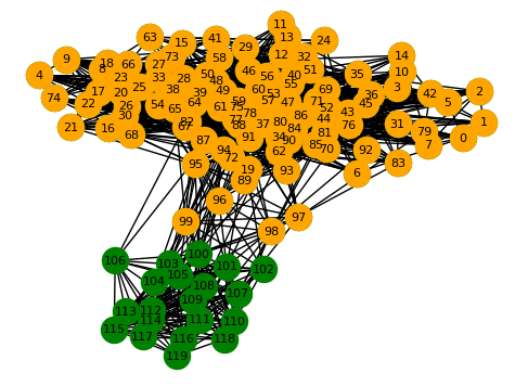
(a)

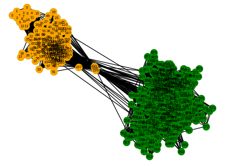
(b)

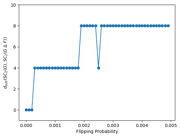
(c)

Figure 5.1: (a) and (b): The social networks we utilized in our experiment were obtained from SNAP. Each node was assigned a color based on the spectral clustering outcomes. (c): We generated 100 graphs from graph (a) and calculated the discrepancy $d_{\text{size}}$ between the outputs of the spectral clustering of the original and perturbed graphs.

Our main theorem ensures that the clustering outcomes remain mostly consistent when edges are flipped with a probability $p<\frac{\log n}{10n}$. The upper bound is about $0.004$ for the first graph and about $0.001$ in the second. We examine $p\in\{0.0001q:1\leq q\leq 50\}$. For each probability $p$ and graph, we create $100$ random graphs $F$ with the given probability. Note that the original graph is represented by $G$. We then compute the difference between the clustering results of $G$ (represented by $\mathcal{SC}_{2}(G)$) and that of $G\triangle F$ (represented by $\mathcal{SC}_{2}(G\triangle F)$).

The chart in Figure 1(c) shows the result we obtain from the first graph. The chart demonstrates the difference between the clustering outputs, represented as $d_{\text{size}}(\mathcal{SC}_{2}(G),\mathcal{SC}_{2}(G\triangle F))$, derived from the $100$ random graphs for each probability. This illustration reveals that, across all considered probabilities, the clustering outcomes remain consistent in every random graph. In each instance, when comparing the original graph to the graph with flipped edges, a minimum of $116$ nodes are assigned to the same clusters. Only a maximum of four nodes out of $120$ experience a change in their cluster placement.

For the second graph, the result is even more robust. For all the probabilities we have conducted the experiment, there were no change in the clustering results by the edge flipping. These two experiments suggest that the clustering results exhibit strong resilience to edge flipping.

6 Concluding Remarks

In this manuscript, we demonstrate and empirically verify that under some assumptions, the spectral clustering algorithm is robust under the randomized response method. While our primary objective is its use in local differential privacy, our validation also confirms the robustness of spectral clustering against social networks containing inaccurate adjacency information.

We demonstrate that the outcomes are robust when $p<\log n/10n$, but also acknowledge that the results can undergo significant alterations for larger $p$ values. This occurs because randomized response introduces an excessive number of edges to the graph in such cases. We are aiming to examine the robustness of other local differential privacy approaches (e.g., as in [32]) that do not add as many edges as the randomized response method. Our results are for the case that we output two clusters from the input graph, but we believe that extending the result to $k$ clusters would be interesting future work.

References

• [1] Cynthia Dwork. Differential privacy: A survey of results. In Theory and Applications of Models of Computation: 5th International Conference, TAMC 2008, Xi’an, China, April 25-29, 2008. Proceedings 5, pages 1–19. Springer, 2008.
• [2] Tianqing Zhu, Gang Li, Wanlei Zhou, and S Yu Philip. Differentially private data publishing and analysis: A survey. IEEE Transactions on Knowledge and Data Engineering, 29(8):1619–1638, 2017.
• [3] Shiva Prasad Kasiviswanathan, Homin K. Lee, Kobbi Nissim, Sofya Raskhodnikova, and Adam Smith. What can we learn privately? SIAM Journal on Computing, 40(3):793–826, 2011.
• [4] Úlfar Erlingsson, Vasyl Pihur, and Aleksandra Korolova. RAPPOR: Randomized aggregatable privacy-preserving ordinal response. In SIGSAC 2014, pages 1054–1067, 2014.
• [5] Apple’s Differential Privacy Team. Learning with privacy at scale. Apple Machine Learning Research, 2017.
• [6] Stanley L. Warner. Randomized response: A survey technique for eliminating evasive answer bias. Journal of the American Statistical Association, 60(309):63–69, 1965.
• [7] Naurang S. Mangat. An improved randomized response strategy. Journal of the Royal Statistical Society: Series B (Methodological), 56(1):93–95, 1994.
• [8] Yue Wang, Xintao Wu, and Donghui Hu. Using randomized response for differential privacy preserving data collection. In EDBT/ICDT Workshops, 2016.
• [9] Jacob Imola, Takao Murakami, and Kamalika Chaudhuri. Communication-Efficient Triangle Counting under Local Differential Privacy. In USENIX Security 2022, pages 537–554, 2022.
• [10] Jacob Imola, Takao Murakami, and Kamalika Chaudhuri. Locally differentially private analysis of graph statistics. In USENIX Security 2021, pages 983–1000, 2021.
• [11] Tianxi Ji, Changqing Luo, Yifan Guo, Qianlong Wang, Lixing Yu, and Pan Li. Community detection in online social networks: A differentially private and parsimonious approach. IEEE Transactions on Computational Social Systems, 7(1):151–163, 2020.
• [12] Mohamed S Mohamed, Dung Nguyen, Anil Vullikanti, and Ravi Tandon. Differentially private community detection for stochastic block models. In International Conference on Machine Learning, pages 15858–15894. PMLR, 2022.
• [13] Nan Fu, Weiwei Ni, Sen Zhang, Lihe Hou, and Dongyue Zhang. GC-NLDP: A graph clustering algorithm with local differential privacy. Computers & Security, 124:102967, 2023.
• [14] Andrew Ng, Michael Jordan, and Yair Weiss. On spectral clustering: Analysis and an algorithm. NIPS 2001, 14, 2001.
• [15] Jonathan Hehir, Aleksandra Slavkovic, and Xiaoyue Niu. Consistent spectral clustering of network block models under local differential privacy. Journal of Privacy and Confidentiality, 12(2), 2022.
• [16] Pan Peng and Yuichi Yoshida. Average sensitivity of spectral clustering. In KDD 2020, pages 1132–1140, 2020.
• [17] Yue Wang, Xintao Wu, and Leting Wu. Differential privacy preserving spectral graph analysis. In PAKDD’13, pages 329–340. Springer, 2013.
• [18] Hongjie Chen, Vincent Cohen-Addad, Tommaso d’Orsi, Alessandro Epasto, Jacob Imola, David Steurer, and Stefan Tiegel. Private estimation algorithms for stochastic block models and mixture models. arXiv preprint arXiv:2301.04822, 2023.
• [19] Kobbi Nissim, Sofya Raskhodnikova, and Adam Smith. Smooth sensitivity and sampling in private data analysis. In STOC 2007, pages 75–84, 2007.
• [20] Yen-Chuen Wei and Chung-Kuan Cheng. Towards efficient hierarchical designs by ratio cut partitioning. In ICCAD 1989, pages 298–301, 1989.
• [21] Lars Hagen and Andrew B Kahng. New spectral methods for ratio cut partitioning and clustering. IEEE Transactions on Computer-Aided Design of Integrated Circuits and Systems, 11(9):1074–1085, 1992.
• [22] Stephen Guattery and Gary L. Miller. On the performance of spectral graph partitioning methods. In SODA 1995, page 233–242, 1995.
• [23] Tsz Chiu Kwok, Lap Chi Lau, Yin Tat Lee, Shayan Oveis Gharan, and Luca Trevisan. Improved Cheeger’s inequality: Analysis of spectral partitioning algorithms through higher order spectral gap. In STOC 2013, pages 11–20, 2013.
• [24] Jeff Cheeger. A Lower Bound for the Smallest Eigenvalue of the Laplacian, pages 195–200. Princeton University Press, Princeton, 1971.
• [25] Noga Alon. Eigenvalues and expanders. Combinatorica, 6(2):83–96, 1986.
• [26] Wassily Hoeffding. Probability inequalities for sums of bounded random variables. Journal of the American Statistical Association, 58(301):13–30, 1963.
• [27] Michael Mitzenmacher and Eli Upfal. Probability and computing: Randomization and probabilistic techniques in algorithms and data analysis. Cambridge University Press, 2017.
• [28] Hermann Weyl. Das asymptotische verteilungsgesetz der eigenwerte linearer partieller differentialgleichungen (mit einer anwendung auf die theorie der hohlraumstrahlung). Mathematische Annalen, 71(4):441–479, 1912.
• [29] Fan Chung and Mary Radcliffe. On the spectra of general random graphs. The Electronic Journal of Combinatorics, pages P215–P215, 2011.
• [30] Paul Erdős, Alfréd Rényi, et al. On the evolution of random graphs. Publ. Math. Inst. Hung. Acad. Sci, 5(1):17–60, 1960.
• [31] Jure Leskovec and Julian Mcauley. Learning to discover social circles in ego networks. NIPS 2012, 25, 2012.
• [32] Maneesh Babu Adhikari, Vorapong Suppakitpaisarn, Arinjita Paul, and C Pandu Rangan. Two-stage framework for accurate and differentially private network information publication. In CSoNet 2020, pages 267–279. Springer, 2020.