Domain Decomposition Method for Poisson–Boltzmann Equations based on Solvent Excluded Surface

Abstract

In this paper, we develop a domain-decomposition method for the generalized Poisson-Boltzmann equation based on a solvent-excluded surface which is widely used in computational chemistry. The solver requires to solve a generalized screened Poisson (GSP) equation defined in $\mathbb{R}^{3}$ with a space-dependent dielectric permittivity and an ion-exclusion function that accounts for Steric effects. Potential theory arguments transform the GSP equation into two-coupled equations defined in a bounded domain. Then, the Schwarz decomposition method is used to formulate local problems by decomposing the cavity into overlapping balls and only solving a set of coupled sub-equations in each ball in which, the spherical harmonics and the Legendre polynomials are used as basis functions in the angular and radial directions. A series of numerical experiments are presented to test the method.

Keywords: Implicit Solvation Model, Poisson-Boltzmann Equation, Domain Decomposition Method, Solvent Excluded Surface, Stern Layer

1 Introduction

In computational chemistry, the nonlinear Poisson Boltzmann (PB) equation is a widely used model for modeling the ionic effects on molecular systems. It belongs to the class of implicit solvation models where the solute is treated microscopically, and the solvent is treated on its macroscopic physical properties, such as dielectric permittivity and ionic strength. Because of this treatment, implicit solvation models are computationally efficient, require fewer parameters, and implicitly consider the sampling over degrees of freedom of the solvent. For this reason, they are widely used in practice and are a popular computational approach to characterize solvent effects in the simulation of properties and processes of molecular systems [55, 49, 40, 54].

The history of the PB model can be traced back to 1910’s where Gouy [18] and Chapman [9] independently used it to equate the chemical potential and relative forces acting on a small adjacent volumes in an ionic solution between two plates having different voltages. Later in 1923, Debye and Hückel generalized the concept by applying it to the theroy of ionic solutions leading to a successful interpretation of thermodynamic data [13]. A combination of both the approaches, including a rigid layer close to the charged surface called the Stern layer and the Gouy-Chapman type diffusive layer was introduced in 1924 by Stern [53]. The PB equations that we consider in this paper is the realization of the Gouy-Chapman model with a possibility of including Stern layer correction [48].

In this paper we consider the nonlinear Poisson-Boltzmann (NPB) equation which is used to describe the dimensionless electrostatic potential $\psi(\boldsymbol{x})$ and is given by

$$-\nabla\cdot\left[\varepsilon(\boldsymbol{x})\nabla\psi(\boldsymbol{x})\right]+\lambda(\boldsymbol{x})\kappa^{2}\varepsilon_{s}\sinh\left(\psi(\boldsymbol{x})\right)=\frac{1}{\beta\varepsilon_{\mathrm{abs}}}\rho^{\mathrm{sol}}(\boldsymbol{x})\qquad\mathrm{in}\quad\Omega_{0}.$$

for the case of $1:1$ electrolyte solvents. Here $\varepsilon(\boldsymbol{x})$ represents the relative space-dependent dielectric permittivity, $\varepsilon_{\mathrm{abs}}$ is the absolute dielectric permittivity of vacuum, $\varepsilon_{s}$ is the relative dielectric permittivity of the solvent, $\rho^{\mathrm{sol}}(\boldsymbol{x})$ is the charge distribution of the solute, $\lambda(\boldsymbol{x})$ is the ion exclusion function that ensures the ion concentration tend to zero inside the solute cavity and one in the solvent region, and $\beta=K_{\mathrm{B}}T/e$, where $K_{\mathrm{B}}$ is the Boltzmann constant, $T$ is the temperature in Kelvins ($K$), and $e$ is the elementary charge.

Some standard numerical methods for solving the PB equation include the finite difference method (FDM), the boundary element method (BEM), and the finite element method (FEM). We briefly overview them and mention some ongoing work in these areas. For an overview of the methods, we refer to [33].

The FDM is one of the most popular methods to solve the linear (LPB) or the nonlinear PB equation. It follows the standard finite difference approach, where a grid covers the region of interest, and then different boundary conditions are chosen. Some of the popular software packages using the FDM include UHBD [34], Delphi [27], MIBPB [10], and APBS [3, 14, 23]. One drawback of this approach is the increase in computational cost with respect to the grid dimension making it challenging to reach high accuracy. Some recent developments in this area can be found in [37, 36, 12].

The BEM is another approach where the LPB equation is recast as an integral equation defined on a two-dimensional solute-solvent interface. This method can be optimized using the fast multipole method or the hierarchical treecode technique. The PAFMPB solver [32, 62] uses the former acceleration technique, whereas the TABI-PB [17, 56] uses the latter one. The PB-SAM solver developed by Head-Gordon et al. [31, 59, 60] discretizes the solute-solvent interface (such as the van der Waals (vdW) surface) with grid points on atomic spheres like a collocation method and solves the associated linear system by use of the fast multipole method. However, one drawback is that integral equation based methods cannot be generalized to NPB. Hybrid approaches combining the FDM and BEM exist [6].

The FEM approach is one of the most flexible approaches for solving the PB equation. It can solve both the linear and the nonlinear PB, providing more flexible mesh refinement and proper convergence analysis [11]. A posteriori error estimation also exists for this method [38, 24]. The SDPBS and SMPBS offer fast and efficient approximations of the size-modified PB equation [57, 61, 22, 58]. Recently a hybrid approach combining the FEM and BEM has been proposed in [7].

Now, we give a brief overview of the domain decomposition methods that have been recently proposed in the context of implicit solvation models. Recently, in [44] a domain decomposition algorithm for the LPB equation (ddLPB) which uses a particular Schwarz domain decomposition method has been developed. A further linear scaling approach for computing the first derivatives and eventually the forces has been presented in [21] following the ideas from [35]. The ideas of the ddLPB method can be traced back to the domain decomposition methods proposed for the conductor-like screening model (COSMO), (ddCOSMO) [8, 28, 29, 30] and the polarizable continuum model (PCM), (ddPCM) [39, 51, 16]. These methods do not require any mesh or grid of the molecular surface, are easy to implement, and about two orders of magnitude faster than the state of the art [29]. In particular, the ddCOSMO solver can perform up to thousands of times faster than equivalent existing algorithms [42, 43]. An open-source software ddX has been released which encompasses all these methods [20].

An essential feature of the implicit solvation model is the choice of the solute-solvent boundary. Most methods use the vdW-cavity or the solvent accessible surface (SAS), [26] as they are topologically simple but they don’t describe the solute-solvent interaction well. The solvent-excluded surface (SES) first developed in [47] is one of the few surfaces which captures the interaction quite well. In [42], a mathematical framework was provided for computing the SES surface. The ddLPB method was developed with the vdW cavity and can be extended to the SAS cavity. The ddPCM method with the SES cavity (ddPCM-SES) was proposed and studied in [43].

In this paper, we incorporate all the ideas mentioned previously. We first present a Schwarz domain decomposition method for the NPB equation that includes steric effects, i.e., the presence of a Stern layer. We use the SES for the solute-solvent boundary and introduce a continuous relative dielectric permittivity function and an ion-exclusion function. As the equation is nonlinear, we develop a nonlinear solver in a unit ball and use spectral methods for discretization using spherical harmonics and Legendre polynomials as basis functions.

The breakdown of the paper is as follows: In Sec. 2, we derive the NPB equation and introduce different solute-solvent boundaries. We also present a continuous relative dielectric permittivity function and an ion-exclusion function based on the SES. In Sec. 3, we transform the problem into different domains and introduce a global strategy for solving them and layout the domain decomposition method. In Sec. 4, we derive single-domain solvers for the homogenous screened Poisson (HSP) and the generalized screened Poisson (GSP) equation in a unit ball. Next, in Sec. 5, we present a comprehensive numerical study for the ddPB-SES method for molecules ranging from one to 24 atoms. Lastly, in Sec. 6, we present a summary and an outlook.

2 Problem Statement

We represent the solvent by a polarizable and ionic continuum. The freedom of the movement of ions is modeled by Boltzmann statistics, i.e., the Boltzmann equation is used to calculate the local ion density $c_{i}$ of the $i^{\mathrm{th}}$ type of ion as follows

$$c_{i}=c_{i}^{\infty}\exp\left(\frac{-W_{i}}{K_{\mathrm{B}}T}\right),$$ (1)

where $c_{i}^{\infty}$ is the bulk ion concentration at an infinite distance from the solute molecule and $W_{i}$ is the work required to move the $i^{\mathrm{th}}$ type of ion to a given position from an infinite distance.

The electrostatic potential $\tilde{\psi}(\boldsymbol{x})$ of a general implicit solvation model is described by the Poisson equation as follows

$$-\nabla\cdot\left[\varepsilon_{\mathrm{abs}}\varepsilon(\boldsymbol{x})\nabla\tilde{\psi}(\boldsymbol{x})\right]=\rho^{\mathrm{sol}}(\boldsymbol{x})+\rho^{\mathrm{ions}}(\boldsymbol{x})\quad\mathrm{in}\ \ \mathbb{R}^{3},$$ (2)

where $\tilde{\psi}(\boldsymbol{x})=\mathcal{O}\left(1/|\boldsymbol{x}|\right)$ as $|\boldsymbol{x}|\rightarrow\infty$. Here $\rho^{\mathrm{ions}}(\boldsymbol{x})$ is the charge distribution of the solvation system.

We derive the PB equation using Eq. (1) and Eq. (2) as

$$-\nabla\cdot\left[\varepsilon_{\mathrm{abs}}\varepsilon(\boldsymbol{x})\nabla\tilde{\psi}(\boldsymbol{x})\right]=\rho^{\mathrm{sol}}(\boldsymbol{x})+\lambda(\boldsymbol{x})\sum_{i=1}^{N_{\mathrm{ions}}}c_{i}^{\infty}z_{i}e\exp\left(\frac{-z_{i}e\tilde{\psi}(\boldsymbol{x})}{K_{\mathrm{B}}T}\right)\quad\mathrm{in}\ \ \mathbb{R}^{3},$$ (3)

where $z_{i}$ is the partial charge of the $i^{\mathrm{th}}$ type of ion.

In the case of a $1:1$ electrolyte, there are two opposite charge ions $(+e$ and $-e)$ and we then get

$$\sum_{i=1}^{2}c_{i}^{\infty}z_{i}e\exp\left(\frac{-z_{i}e\tilde{\psi}(\boldsymbol{x})}{K_{\mathrm{B}}T}\right) =ce\exp\left(\frac{-e\tilde{\psi}(\boldsymbol{x})}{K_{\mathrm{B}}T}\right)-ce\exp\left(\frac{e\tilde{\psi}(\boldsymbol{x})}{K_{\mathrm{B}}T}\right)$$

$$=-2ce\sinh\left(\frac{e\tilde{\psi}(\boldsymbol{x})}{K_{\mathrm{B}}T}\right).$$ (4)

Then substituting Eq. (2) into Eq. (3) we obtain

$$-\nabla\cdot\left[\varepsilon_{\mathrm{abs}}\varepsilon(\boldsymbol{x})\nabla\tilde{\psi}(\boldsymbol{x})\right]+\lambda(\boldsymbol{x})2ce\sinh\left(\frac{e\tilde{\psi}(\boldsymbol{x})}{K_{\mathrm{B}}T}\right)=\rho^{\mathrm{sol}}(\boldsymbol{x})\quad\mathrm{in}\ \ \mathbb{R}^{3},$$ (5)

the nonlinear Poisson-Boltzmann equation (NPB).

2.1 Solute Probe

One of the important properties for implicit solvation model is the choice of the solute probe and, accordingly, the solute-solvent boundary. A straightforward choice is using the van der Waals (vdW) surface, i.e., the topological boundary of the union of solute’s vdW-atoms with experimentally fitted radii. Another choice is the solvent-accessible surface (SAS), which is defined by tracing the center of an idealized (spherical) solvent probe (representing a solvent molecule) when rolling over the solute molecule. The region enclosed by the SAS is called the SAS-cavity, which we denote by $\Omega_{\mathrm{SAS}}$ and its boundary by $\Gamma_{\mathrm{SAS}}$.

The vdW and the SAS are topologically not the correct answer to the cavity problem as they poorly describe the region where the solvent can touch. However, as they are topologically simple, they are widely used in numerical computations. Another solute-solvent boundary is the solvent-excluded surface (SES), which represents the boundary of the region where the probe has no access due to the presence of the solute. The region enclosed by the SES is the SES cavity, that we denote by $\Omega_{\mathrm{SES}}$ and the boundary by $\Gamma_{\mathrm{SES}}$. The mathematical characterization of the surface can be found in [42].

The PB equation do not consider the absorbing ions finite size; hence, the ionic concentration can exceed the maximally allowed coverage near the surface. These are referred to as steric effects. To account for these steric effects, the PB model is modified to include a Stern layer, [5]. We introduce two cavities, namely the solvent-excluded surface including the steric effect (SES-S) and the solvent-accessible surface including steric effects (SAS-S), which will be denoted by $\Omega_{\mathrm{SES-S}}$ and $\Omega_{\mathrm{SAS-S}}$ respectively with the corresponding boundary being $\Gamma_{\mathrm{SES-S}}$ and $\Gamma_{\mathrm{SAS-S}}$. Fig. 1 represents all the molecular probes and the boundaries introduced.

Figure 1: Solute probes and solute-solvent boundary for a molecule.

Now, we set certain notations. We assume that the molecule is composed of $M$ atoms and the $i^{\mathrm{th}}$ atom has center $\boldsymbol{x}_{i}$ and vdW radii $r_{i}$. The solvent probe radius is denoted by $r_{p}$. Furthermore, for each atom, we define an “enlarged” ball $\Omega_{i}$ with center $\boldsymbol{x}_{i}$ and radius $R_{i}=r_{i}+r_{p}+a+r_{0}$, where $a$ is the Stern layer length, and $r_{0}$ is a non-negative constant use to control the nonlinear regime. For the inclusion of the Steric effects we assume that the SAS cavity is formed with a probe of radius $a+r_{p}$.

The SES cavity is entirely covered by the union of $\Omega_{0}$ of enlarged balls, i.e.,

$$\Omega_{\mathrm{SES}}\subset\Omega_{0}:=\bigcup_{i=1}^{M}\Omega_{i},\quad\mathrm{where}\quad\Omega_{i}=B_{R_{i}}(\boldsymbol{x}_{i}).$$

We also denote the solvent region by $\Omega_{\infty}:=\mathbb{R}^{3}\setminus\Omega_{0}=\Omega_{0}^{\mathrm{C}}$.

Let $f_{\mathrm{SAS}}$ denote the distance function to $\Omega_{\mathrm{SAS}}$ (i.e., negative inside the SAS cavity and positive outside the SAS cavity). We then have a mathematical characterization of the two cavities

$$\Omega_{\mathrm{SES}}=\left\{\boldsymbol{x}\in\mathbb{R}^{3}:\ f_{\mathrm{SAS}}(\boldsymbol{x})\leq-r_{p}-a\right\}\ \ \mathrm{and}\ \ \Omega_{0}=\left\{\boldsymbol{x}\in\mathbb{R}^{3}:\ f_{\mathrm{SAS}}(\boldsymbol{x})\leq r_{0}\right\}.$$

Also, we can characterize their boundary surfaces by

$$\Gamma_{\mathrm{SES}}=f^{-1}_{\mathrm{SAS}}(-r_{p}-a)\quad\mathrm{and}\quad\Gamma_{0}=f^{-1}_{\mathrm{SAS}}(r_{0}).$$

Remark 1

It is reasonable to assume that the solute’s charge distribution $\rho^{\mathrm{sol}}$ is supported in $\Omega_{0}$. In this paper we consider the classic description of $\rho^{\mathrm{sol}}$ given by

$$\rho^{\mathrm{sol}}(\boldsymbol{x})=\sum_{i=1}^{M}q_{i}\delta(\boldsymbol{x}-\boldsymbol{x}_{i}),$$

where $q_{i}$ denotes the (partial) charge carried by the $i^{\mathrm{th}}$ atom, and $\delta$ is the Dirac-delta function. For a quantum description of the solute, $\rho^{\mathrm{sol}}$ comprises of a sum of nuclear charges and the electron charge density.

2.2 Dielectric Permittivity and Ion Exclusion Function

In this subsection we construct a SES-based dielectric permittivity and an ion-exclusion function associated with $f_{\mathrm{SAS}}$ which follows the ideas from [43].

It is assumed that the solvent dielectric permittivity is constant and equal to the bulk dielectric permittivity outside the $\mathrm{SAS}$ cavity. This is a reasonable assumption as the solvent density at positions far from the solute molecule is approximately the same, and therefore the dielectric permittivity is the same.

Taking the SES as the solute-solvent boundary implies that the dielectric permittivity in the SES-cavity is always one, i.e., the relative dielectric of vacuum and constant outside $\mathrm{SAS}$, with value $\varepsilon_{s}$. Let us denote the layer between $\Omega_{\mathrm{SAS}}$ and $\Omega_{\mathrm{SES}}$ by $\mathcal{L}_{\varepsilon}$, i.e., $\mathcal{L}_{\varepsilon}:=\Omega_{\mathrm{SAS}}\setminus\Omega_{\mathrm{SES}}$. In a similar way the ion-exclusion function is zero inside $\Omega_{\mathrm{SES-S}}$ and one outside $\Omega_{\mathrm{SAS-S}}$. We denote the layer between $\Omega_{\mathrm{SES-S}}$ and $\Omega_{\mathrm{SAS-S}}$ by $\mathcal{L}_{\lambda}$, i.e., $\mathcal{L}_{\lambda}=\Omega_{\mathrm{SAS-S}}\setminus\Omega_{\mathrm{SES-S}}$.

The remaining work is to determine $\varepsilon(\boldsymbol{x})$ and $\lambda(\boldsymbol{x})$ in the intermediate layer, $\mathcal{L}_{\varepsilon}$ and $\mathcal{L}_{\lambda}$, respectively. We choose the following modified definition of the permittivity function from [43],

$$\varepsilon(\boldsymbol{x})=\left\{\begin{array}[]{ll}1&\boldsymbol{x}\in\Omega_{\mathrm{SES}},\\ 1+(\varepsilon_{s}-1)\xi\left(\dfrac{f_{\mathrm{SAS}}(\boldsymbol{x})+r_{p}+a}{r_{p}+a}\right)&\boldsymbol{x}\in\mathcal{L}_{\varepsilon},\\ \varepsilon_{s}&\mathrm{else},\end{array}\right.$$ (6)

and define the ion exclusion function as

$$\lambda(\boldsymbol{x})=\left\{\begin{array}[]{ll}0&\boldsymbol{x}\in\Omega_{\mathrm{SES-S}},\\ \xi\left(\dfrac{f_{\mathrm{SAS}}(\boldsymbol{x})+r_{p}}{r_{p}+a}\right)&\boldsymbol{x}\in\mathcal{L}_{\lambda},\\ 1&\mathrm{else},\end{array}\right.$$ (7)

where $\xi(\cdot)$ is a continuous function defined on $[0,1]$, satisfying $\xi(0)=0$, $\xi(1)=1$, $\xi^{\prime}(0)=0$, and $\xi^{\prime}(1)=0$. $\varepsilon(\boldsymbol{x})$ and $\lambda(\boldsymbol{x})$ can be seen as distance-dependent functions where the “distance” represents the signed distance to SAS, see Fig. 2 for a schematic diagram. The function $\xi(\cdot)$ can be chosen in different ways. In [52] one possible choice is the error function, $\mathtt{erf}(\cdot)$. In the numerical simulations we choose

$$\xi(t)=t^{3}\left(10+3t\left(-5+2t\right)\right),\qquad 0\leq t\leq 1.$$

Remark 2

We also define an enlarged cavity $\mathcal{L}:=\Omega_{0}\setminus\Omega_{\mathrm{SES}}$. By the definition of $\mathcal{L}_{\varepsilon}$ and $\mathcal{L}_{\lambda}$ we have an immediate consequence of $\mathcal{L}_{\lambda}\subset\mathcal{L}$ and $\mathcal{L}_{\varepsilon}\subset\mathcal{L}$.

Figure 2: Schematic diagram of the dielectric permittivity, $\varepsilon(\boldsymbol{x})$ (left $y$-axis) and the ion-exclusion function, $\lambda(\boldsymbol{x})$ (right $y$-axis) with respect to $f_{\mathrm{SAS}}$.

3 Formulation of the Problem

In this section we reduce our problem to different domains by introducing a new hybrid linear/nonlinear PB model and introduce the domain decomposition strategy use to solve the resulting equation.

In the previous section we introduced the dielectric permittivity function and the ion-exclusion function. Let $\psi=e\tilde{\psi}/K_{\mathrm{B}}T$ denote the dimensionless electrostatic potential then the fully nonlinear PB equation reduces to

$$-\nabla\cdot\left[\varepsilon_{\mathrm{abs}}\varepsilon(\boldsymbol{x})\nabla\beta\psi(\boldsymbol{x})\right]+\lambda(\boldsymbol{x})2ce\sinh\left(\psi(\boldsymbol{x})\right)=\rho^{\mathrm{sol}}(\boldsymbol{x})\quad\mathrm{in}\ \ \mathbb{R}^{3}.$$ (8)

Since the support of $\rho^{\mathrm{sol}}(\boldsymbol{x})$ is contained in $\Omega_{0}$, i.e., $\mathrm{supp}(\rho^{\mathrm{sol}})\subset\Omega_{0}$, by using the definition of $\varepsilon(\boldsymbol{x})$ and $\lambda(\boldsymbol{x})$, Eq. (8) reduces to

$$-\varepsilon_{s}\varepsilon_{\mathrm{abs}}\beta\Delta\psi(\boldsymbol{x})+2ce\sinh\left(\psi(\boldsymbol{x})\right)=0\quad\mathrm{in}\ \ \Omega_{\infty}.$$

In the solvent region $\Omega_{\infty}$, we can assume that the potential $\psi$ satisfies the low potential condition, i.e., $|\psi|\ll 1$, and hence we can linearise the above equation to get a homogeneous screened Poisson (HSP) equation as

$$-\Delta\psi(\boldsymbol{x})+\kappa^{2}\psi(\boldsymbol{x})=0\quad\ \ \mathrm{in}\ \ \Omega_{\infty},$$ (9)

where $\kappa^{2}=2e^{2}c/K_{\mathrm{B}}T\varepsilon_{s}\varepsilon_{\mathrm{abs}}$ is the square of the Debye Hückel screening constant.

Next we note that inside the cavity $\Omega_{0}$ we still keep the nonlinear Poisson Boltzmann equation of the form

$$-\nabla\cdot\left[\varepsilon(\boldsymbol{x})\nabla\psi(\boldsymbol{x})\right]+\lambda(\boldsymbol{x})\kappa^{2}\varepsilon_{s}\sinh\left(\psi(\boldsymbol{x})\right)=\frac{1}{\beta\varepsilon_{\mathrm{abs}}}\rho^{\mathrm{sol}}(\boldsymbol{x})\quad\mathrm{in}\ \ \Omega_{0}.$$ (10)

Along the solute-solvent boundary $\Gamma_{0}$, equations (9)–(10) satisfy the jump conditions

$$\left[\![\psi]\!\right]=0,\qquad\left[\![\partial_{\boldsymbol{n}}\psi]\!\right]=0\quad\mathrm{on}\quad\Gamma_{0}:=\partial\Omega_{0},$$ (11)

where $\boldsymbol{n}$ is the unit normal vector on $\Gamma_{0}$ pointing outward and $\partial_{\boldsymbol{n}}=\nabla\cdot\boldsymbol{n}$, i.e., the normal derivative which complete the hybrid linear/nonlinear model.

Remark 3

We notice that we reduced our problem defined on the whole space $\mathbb{R}^{3}$ to the solute cavity $\Omega_{0}$ and the solvent region $\Omega_{\infty}$ but with non-local coupling conditions. Fig. 3 shows the schematic diagram of PDEs in different regions.

Figure 3: PDEs defined in the solute cavity and the solvent region.

3.1 Transformation of the Problem

We noticed that we have two equations defined in $\mathbb{R}^{3}$, one inside the cavity, $\Omega_{0}$ and one in the solvent region $\Omega_{\infty}$ in combination with interface conditions. In this subsection we transform our problem and define them as two coupled PDEs in $\Omega_{0}$.

Let us denote $\psi|_{\Omega_{\infty}}$ as the Dirichlet trace from $H^{1}(\Omega_{\infty})$ to $L^{2}(\partial\Omega_{\infty})$ in the sense of the trace operator, then by the linearity of Eq. (9) we notice that the free-space electrostatic potential $\psi|_{\Omega_{\infty}}$ can be represented by a single-layer potential, $\tilde{\mathcal{S}}_{\Gamma_{0}}:H^{-1/2}(\Gamma_{0})\rightarrow H^{1}(\mathbb{R}^{3}\setminus\Gamma_{0})$ as

$$\psi(\boldsymbol{x})|_{\Omega_{\infty}}=\tilde{\mathcal{S}}_{\Gamma_{0}}\sigma_{\mathrm{e}}(\boldsymbol{x})\quad\forall\ \boldsymbol{x}\in\Omega_{\infty},$$

where $\sigma_{\mathrm{e}}(\boldsymbol{x})$ is a distribution in $H^{-1/2}(\Gamma_{0})$. From the continuity of the single layer potential operator we can extend $\psi|_{\Omega_{\infty}}$ to $\Omega_{0}$ as follows:

$$\psi_{\mathrm{e}}(\boldsymbol{x})=\int_{\Gamma_{0}}\frac{\exp\left(-\kappa|\boldsymbol{x}-\boldsymbol{y}|\right)\sigma_{\mathrm{e}}(\boldsymbol{y})}{4\pi|\boldsymbol{x}-\boldsymbol{y}|}d\boldsymbol{y}\quad\forall\ \boldsymbol{x}\in\Omega_{0},$$

where $\psi_{\mathrm{e}}(\boldsymbol{x})$ denotes the extended potential and hence $\psi_{\mathrm{e}}$ satisfies the HSP equation in $\Omega_{\infty}$ and also satisfies

$$-\Delta\psi_{\mathrm{e}}(\boldsymbol{x})+\kappa^{2}\psi_{\mathrm{e}}(\boldsymbol{x})=0\quad\mathrm{in}\ \ \Omega_{0}.$$

Here we also introduce the single-layer potential operator $\mathcal{S}_{\Gamma_{0}}:H^{-1/2}(\Gamma_{0})\rightarrow H^{1/2}(\Gamma_{0})$ defined by

$$\mathcal{S}_{\Gamma_{0}}\sigma_{\mathrm{e}}(\boldsymbol{x}):=\int_{\Gamma_{0}}\frac{\exp\left(-\kappa|\boldsymbol{x}-\boldsymbol{y}|\right)\sigma_{\mathrm{e}}(\boldsymbol{y})}{4\pi|\boldsymbol{x}-\boldsymbol{y}|}d\boldsymbol{y}\quad\forall\boldsymbol{x}\in\Gamma_{0},$$ (12)

which is an invertible operator and hence $\sigma_{\mathrm{e}}=\mathcal{S}_{\Gamma_{0}}^{-1}\psi|_{\Gamma_{0}}$.

From [50, Theorem 3.3.1] we also have the relationship

$$\sigma_{\mathrm{e}}=\partial_{\boldsymbol{n}}\psi_{\mathrm{e}}|_{\Omega_{0}}-\partial_{\boldsymbol{n}}\psi_{\mathrm{e}}|_{\Omega_{\infty}}\quad\mathrm{on}\quad\Gamma_{0}.$$

By the jump condition (Eq. (11)) of the normal derivative we have

$$\partial_{\boldsymbol{n}}\psi|_{\Omega_{\infty}}-\partial_{\boldsymbol{n}}\psi|_{\Omega_{0}}=0\quad\ \ \mathrm{on}\ \ \Gamma_{0},$$

which implies $\partial_{\boldsymbol{n}}\psi_{\mathrm{e}}|_{\Omega_{\infty}}=\partial_{\boldsymbol{n}}\psi|_{\Omega_{0}}$ on $\Gamma_{0}$. Hence,

$$\sigma_{\mathrm{e}}=\partial_{\boldsymbol{n}}\left(\psi_{\mathrm{e}}|_{\Omega_{0}}-\psi|_{\Omega_{0}}\right)\quad\mathrm{on}\ \ \Gamma_{0}.$$

Also, by the jump condition of the potential we get $\psi_{\mathrm{e}}=\psi|_{\Omega_{0}}$ on $\Gamma_{0}$. Hence, the extended potential $\psi_{\mathrm{e}}$ is defined on $\Omega_{0}$ by

$$-\Delta\psi_{\mathrm{e}}(\boldsymbol{x})+\kappa^{2}\psi_{\mathrm{e}}(\boldsymbol{x}) =0 \quad\mathrm{in}\quad\Omega_{0}$$

$$\psi_{\mathrm{e}}(\boldsymbol{x}) =\psi(\boldsymbol{x}) \quad\mathrm{on}\quad\Gamma_{0}.$$

Now, we move towards the generalized NPB equation. Let $\psi_{0}(\boldsymbol{x})$ denote the potential generated by $\rho^{\mathrm{sol}}(\boldsymbol{x})/\beta\varepsilon_{\mathrm{abs}}$ in vacuum, i.e.,

$$\psi_{0}(\boldsymbol{x})=\sum_{i=1}^{M}\frac{q_{i}}{4\pi\varepsilon_{\mathrm{abs}}\beta|\boldsymbol{x}-\boldsymbol{x}_{i}|},$$

satisfying

$$-\Delta\psi_{0}=\frac{1}{\beta\varepsilon_{\mathrm{abs}}}\rho^{\mathrm{sol}}(\boldsymbol{x})\quad\mathrm{in}\ \ \mathbb{R}^{3}.$$ (13)

Let us denote the reaction potential by, $\psi_{\mathrm{r}}:=\psi-\psi_{0}$, i.e., the difference between the electrostatic potential with and without the presence of solvent. Then Eq. (10) equivalently writes

$$-\nabla\cdot\left[\varepsilon(\boldsymbol{x})\nabla\psi_{\mathrm{r}}(\boldsymbol{x})\right] +\lambda(\boldsymbol{x})\kappa^{2}\varepsilon_{s}\sinh\left(\left(\psi_{\mathrm{r}}+\psi_{0}\right)(\boldsymbol{x})\right)$$

$$=\frac{1}{\beta\varepsilon_{\mathrm{abs}}}\rho^{\mathrm{sol}}(\boldsymbol{x})+\nabla\cdot\left[\varepsilon(\boldsymbol{x})\nabla\psi_{0}(\boldsymbol{x})\right] \qquad\mathrm{in}\ \ \Omega_{0}.$$ (14)

Substituting Eq. (13) in Eq. (3.1) and denoting $\sinh(\Phi)$ by $\mathcal{F}(\Phi)\Phi$ where

$$\mathcal{F}(\Phi)=\frac{\sinh(\Phi)}{\Phi},$$

for any positive function $\Phi$. We further reduce the equation to

$$-\nabla\cdot\left[\varepsilon(\boldsymbol{x})\nabla\psi_{\mathrm{r}}(\boldsymbol{x})\right] +\lambda(\boldsymbol{x})\kappa^{2}\varepsilon_{s}\mathcal{F}\left((\psi_{\mathrm{r}}+\psi_{0})(\boldsymbol{x})\right)\left(\psi_{\mathrm{r}}+\psi_{0}\right)(\boldsymbol{x})$$

$$=\nabla\cdot\left[\left(\varepsilon(\boldsymbol{x})-1\right)\nabla\psi_{0}(\boldsymbol{x})\right]\qquad \mathrm{in}\ \ \Omega_{0}.$$

From the jump condition,, $\left[\![\psi]\!\right]=0$ we have $\psi|_{\Omega_{0}}-\psi|_{\Omega_{\infty}}=0$ which implies

$$\psi_{\mathrm{r}}+\psi_{0}=\psi_{\mathrm{e}}\quad\mathrm{on}\ \ \Gamma_{0},$$

and similarly

$$\sigma_{\mathrm{e}}=\partial_{\boldsymbol{n}}\psi_{\mathrm{e}}-\partial_{\boldsymbol{n}}\left(\psi_{\mathrm{r}}+\psi_{0}\right)\quad\mathrm{on}\ \ \Gamma_{0}.$$

From Eq. (12) we also get the global coupling condition

$$\psi_{\mathrm{e}}(\boldsymbol{x})=\mathcal{S}_{\Gamma_{0}}\sigma_{\mathrm{e}}=\mathcal{S}_{\Gamma_{0}}\left[\partial_{\boldsymbol{n}}\psi_{\mathrm{e}}-\partial_{\boldsymbol{n}}\left(\psi_{\mathrm{r}}+\psi_{0}\right)\right]\quad\mathrm{on}\ \ \Gamma_{0}.$$

In summary our original equation reduces to

$$-\nabla\cdot\left[\ \varepsilon(\boldsymbol{x})\nabla\psi_{\mathrm{r}}(\boldsymbol{x})\right] +\lambda(\boldsymbol{x})\kappa^{2}\varepsilon_{s}\mathcal{F}\left((\psi_{\mathrm{r}}+\psi_{0})(\boldsymbol{x})\right)\left(\psi_{\mathrm{r}}+\psi_{0}\right)(\boldsymbol{x})$$

$$=\nabla\cdot\left[\left(\varepsilon(\boldsymbol{x})-1\right)\nabla\psi_{0}(\boldsymbol{x})\right] \mathrm{in}\ \ \Omega_{0},$$ (15)

$$-\Delta\psi_{\mathrm{e}}(\boldsymbol{x})+\kappa^{2}\psi_{\mathrm{e}}(\boldsymbol{x}) =0 \mathrm{in}\ \ \Omega_{0},$$ (16)

with two coupling conditions given on $\Gamma_{0}$ by

$$\left(\psi_{\mathrm{r}}+\psi_{0}\right)(\boldsymbol{x}) =\psi_{\mathrm{e}}(\boldsymbol{x}) \quad\mathrm{on}\ \ \Gamma_{0},$$ (17)

$$\psi_{\mathrm{e}}(\boldsymbol{x}) =g \quad\mathrm{on}\ \ \Gamma_{0},$$ (18)

where

$$g=\mathcal{S}_{\Gamma_{0}}\sigma_{\mathrm{e}}=\mathcal{S}_{\Gamma_{0}}\left[\partial_{\boldsymbol{n}}\psi_{\mathrm{e}}-\partial_{\boldsymbol{n}}\left(\psi_{\mathrm{r}}+\psi_{0}\right)\right]\quad\mathrm{on}\ \ \Gamma_{0}.$$ (19)

Remark 4

The PDEs defined in Eq. (15)–(16) encompass different solvation models. In the absence of Stern layer, constant discontinuous dielectric permittivity function, and the solute probe given by the vdW surface the model is reduced to the linear Poisson Boltzmann (LPB). If $\kappa\rightarrow 0$ then we recover the polarizable continuum model with SES boundary (PCM-SES). For the vdW surface, we get the classical PCM model. Lastly, for $\kappa\rightarrow\infty$ the model tends to the conductor line screening model (COSMO) which is reasonable as then the solvent becomes a perfect conductor as the ionic strength tends to $\infty$ and screens any change from the solute. Domain decomposition algorithms for all the four methods denoted by ddLPB, ddPCM-SES, ddPCM, and ddCOSMO can be found in [44, 43, 51, 8], respectively.

3.2 Global Strategy

For solving Eq. (15)–(16) we follow the same ideas as prescribed in [43, 44]. Let $g^{(0)}$ be an initial guess for the Dirichlet condition $\psi_{\mathrm{e}}|_{\Gamma_{0}}$ and set $\mathtt{k}=1$:

1. Solve the following nonlinear Dirichlet boundary problem for $\psi_{\mathrm{r}}^{(\mathtt{k})}$:

   $$-\nabla\cdot\left[\varepsilon(\boldsymbol{x})\nabla\psi_{\mathrm{r}}^{(\mathtt{k})}(\boldsymbol{x})\right] +\lambda(\boldsymbol{x})\kappa^{2}\varepsilon_{s}\mathcal{F}\left((\psi_{\mathrm{r}}^{(\mathtt{k})}+\psi_{0})\right)\left(\psi_{\mathrm{r}}^{(\mathtt{k})}+\psi_{0}\right)(\boldsymbol{x})$$

   $$=\nabla\cdot\left[\left(\varepsilon(\boldsymbol{x})-1\right)\nabla\psi_{0}(\boldsymbol{x})\right]\qquad \mathrm{in}\ \ \Omega_{0},$$

   $$\psi_{\mathrm{r}}^{(\mathtt{k})}(\boldsymbol{x}) =g^{(\mathtt{k}-1)}-\psi_{0}(\boldsymbol{x})\qquad \mathrm{on}\ \ \Gamma_{0},$$

   and derive the Neumann trace $\partial_{\boldsymbol{n}}\psi_{\mathrm{r}}^{(\mathtt{k})}$ on $\Gamma_{0}$.

2. Solve the Dirichlet boundary problem for $\psi_{\mathrm{e}}^{(\mathtt{k})}$:

   $$-\Delta\psi_{\mathrm{e}}^{(\mathtt{k})}(\boldsymbol{x})+\kappa^{2}\psi_{\mathrm{e}}^{(\mathtt{k})}(\boldsymbol{x}) =0\qquad \mathrm{in}\ \ \Omega_{0},$$

   $$\psi_{\mathrm{e}}^{(\mathtt{k})}(\boldsymbol{x}) =g^{(\mathtt{k}-1)}\qquad \mathrm{on}\ \ \Gamma_{0},$$

   and derive the Neumann trace $\partial_{\boldsymbol{n}}\psi_{\mathrm{e}}^{(\mathtt{k})}$ on $\Gamma_{0}$.

3. Build the charge density $\sigma_{\mathrm{e}}^{(\mathtt{k})}=\partial_{\boldsymbol{n}}\psi_{\mathrm{e}}^{(\mathtt{k})}-\partial_{\boldsymbol{n}}\left(\psi_{0}+\psi_{\mathrm{r}}^{(\mathtt{k})}\right)$ and compute a new Dirichlet condition $g^{(\mathtt{k})}=\mathcal{S}_{\Gamma_{0}}\sigma_{\mathrm{e}}^{(\mathtt{k})}$.

4. Compute the contribution $E^{\mathtt{k}}_{s}$ to the solvation energy based on $\psi_{\mathrm{r}}^{(\mathtt{k})}$ at the $\mathtt{k}^{\mathrm{th}}$ iteration step, set $\mathtt{k}\rightarrow\mathtt{k}+1$, go back to $\mathtt{[1]}$ and repeat until $|E^{\mathtt{k}}_{s}-E^{\mathtt{k}-1}_{s}|/|E^{\mathtt{k}}_{s}|<\mathtt{tol}$ for $\mathtt{tol}\ll 1$.

In the above algorithm $E^{\mathtt{k}}_{s}$ denotes the electrostatic solvation energy at iteration $\mathtt{k}$ which will be defined in Sec. 5.

Remark 5

For choosing a suitable guess to $g^{(0)}$ (defined on $\Gamma_{0}$) we consider the (unrealistic) situation when the whole space $\mathbb{R}^{3}$ is covered by the solvent medium. Then the electrostatic potential $\psi$ would be given by

$$\psi(\boldsymbol{x})=\sum_{i=1}^{M}\frac{q_{i}}{\beta\varepsilon_{s}}\frac{\exp\left(-\kappa|\boldsymbol{x}-\boldsymbol{x}_{i}|\right)}{4\pi\varepsilon_{\mathrm{abs}}|\boldsymbol{x}-\boldsymbol{x}_{i}|}\quad\forall\ \ \boldsymbol{x}\in\mathbb{R}^{3},$$

see [25, Sec 1.3.2]. Hence $g^{(0)}$ is chosen as this potential restricted to $\Gamma_{0}$.

Remark 6

We note that the global strategy is an iterative process. The final convergent solution satisfies, after discretisation, a global nonlinear system that can be solved. Unlike the LPB approach the solution of the nonlinear problem in Step $\mathtt{[1]}$ needs to be studied properly and will be discussed in Remark 8.

3.3 Domain Decomposition Strategy

In this work we will consider the Schwarz domain decomposition method [45] as it is aimed at solving PDEs defined on complex domain which can be decomposed as a union of overlapping and simple sub-domain. The main idea is to solve in each sub-domain the same equation but with boundary conditions that depend on the global boundary conditions and on the solution of neighboring domains.

We recall that we have a natural decomposition of $\Omega_{0}$ as follows

$$\Omega_{0}=\bigcup_{j=1}^{M}\Omega_{j},\quad\Omega_{j}=B_{R_{j}}(\boldsymbol{x}_{j}),$$

where $\boldsymbol{x}_{j}$ is the center of ball $\Omega_{j}$ and $R_{j}=r_{j}+r_{p}+r_{0}+a$. We replace the global equation (15)–(16) by the following coupled equations, each restricted to $\Omega_{j}$,

$$-\nabla\cdot\left[\varepsilon(\boldsymbol{x})\nabla\psi_{\mathrm{r}}|_{\Omega_{j}}(\boldsymbol{x})\right] +\lambda(\boldsymbol{x})\kappa^{2}\varepsilon_{s}\mathcal{F}\left((\psi_{\mathrm{r}}|_{\Omega_{j}}+\psi_{0})\right)\left(\psi_{\mathrm{r}}|_{\Omega_{j}}+\psi_{0}\right)(\boldsymbol{x})$$

$$=\nabla\cdot\left[\left(\varepsilon(\boldsymbol{x})-1\right)\nabla\psi_{0}(\boldsymbol{x})\right]\qquad \mathrm{in}\ \ \Omega_{j},$$

$$\psi_{\mathrm{r}}|_{\Omega_{j}}(\boldsymbol{x}) =h_{\mathrm{r},j}\quad \mathrm{on}\ \ \Gamma_{j},$$ (20)

with

$$h_{\mathrm{r},j}=\left\{\begin{array}[]{lll}\psi_{\mathrm{r}}&\mathrm{on}&\Gamma_{j}^{\mathtt{i}}\\ g-\psi_{0}&\mathrm{on}&\Gamma_{j}^{\mathtt{e}}.\end{array}\right.$$ (21)

Here, $\Gamma_{j}^{\mathtt{e}}$ is the external part of $\Gamma_{j}$ not contained in any other $\Omega_{i}\ (i\neq j)$, i.e., $\Gamma_{j}^{\mathtt{e}}=\Gamma_{0}\cap\Gamma_{j}$, and $\Gamma_{j}^{\mathtt{i}}$ is the internal part of $\Gamma_{j}$, i.e., $\Gamma_{j}^{\mathtt{i}}=\Omega\cap\Gamma_{j}$ (see Fig. 4).

Figure 4: 2-D schematic diagram of $\Gamma_{j}^{\mathtt{i}}$ and $\Gamma_{i}^{\mathtt{e}}$.

Similarly the equations for the extended potential are

$$-\Delta\psi_{\mathrm{e}}|_{\Omega_{j}}(\boldsymbol{x})+\kappa^{2}\psi_{\mathrm{e}}|_{\Omega_{j}}(\boldsymbol{x}) =0\qquad \mathrm{in}\ \ \Omega_{j},$$

$$\psi_{\mathrm{e}}|_{\Omega_{j}}(\boldsymbol{x}) =h_{\mathrm{e},j}\qquad \mathrm{on}\ \ \Gamma_{j},$$ (22)

with

$$h_{\mathrm{e},j}=\left\{\begin{array}[]{lll}\psi_{\mathrm{e}}&\mathrm{on}&\Gamma_{j}^{\mathtt{i}}\\ g&\mathrm{on}&\Gamma_{j}^{\mathtt{e}}.\end{array}\right.$$ (23)

Remark 7

The Dirichlet boundary conditions in Eq. (3.3)–(3.3) are implicit since $\psi_{\mathrm{r}}$ (respectively $\psi_{\mathrm{e}}$) is not known on $\Gamma_{j}^{\mathtt{i}}$. Hence, one needs to use an iterative scheme to solve Eq. (3.3)–(21) (respectively Eq. (3.3)–(23)), such as the parallel Schwarz algorithm or the alternating Schwarz algorithm as presented in for ddCOSMO in [8]. The visual overview of the domain decomposition algorithm is presented in Fig. 5.

Remark 8

We note that in Eq. (3.3) we have a nonlinearity because of the term

$$\lambda(\boldsymbol{x})\kappa^{2}\varepsilon_{s}\mathcal{F}\left((\psi_{\mathrm{r}}|_{\Omega_{j}}+\psi_{0})\right)\left(\psi_{\mathrm{r}}|_{\Omega_{j}}+\psi_{0}\right)(\boldsymbol{x}).$$ (24)

A standard way of solving such nonlinear equations after discretisation is the use of a fixed point technique and replace Eq. (24) by

$$\lambda(\boldsymbol{x})\kappa^{2}\varepsilon_{s}\mathcal{F}\left((\psi_{\mathrm{r}}|_{\Omega_{j}}^{(\nu-1)}+\psi_{0})\right)\left(\psi_{\mathrm{r}}|_{\Omega_{j}}^{(\nu)}+\psi_{0}\right)(\boldsymbol{x}).$$

where $\psi_{\mathrm{r}}^{(\nu-1)}(\boldsymbol{x})$ denotes the solution at the $(\nu-1)^{\mathrm{th}}$ iterative step. As $\psi_{\mathrm{r}}^{(\nu-1)}(\boldsymbol{x})$ is known throughout the derivation we replace Eq. (3.3) by the linear counterpart

$$-\nabla\cdot\left[\varepsilon(\boldsymbol{x})\nabla\psi_{\mathrm{r}}|_{\Omega_{j}}(\boldsymbol{x})\right] +\lambda(\boldsymbol{x})\kappa^{2}\varepsilon_{s}\mathcal{F}\left((\overline{\psi_{\mathrm{r}}}|_{\Omega_{j}}+\psi_{0})\right)\left(\psi_{\mathrm{r}}|_{\Omega_{j}}+\psi_{0}\right)(\boldsymbol{x})$$

$$=\nabla\cdot\left[\left(\varepsilon(\boldsymbol{x})-1\right)\nabla\psi_{0}(\boldsymbol{x})\right]\qquad \mathrm{in}\ \ \Omega_{j}$$

$$\psi_{\mathrm{r}}|_{\Omega_{j}}(\boldsymbol{x}) =h_{\mathrm{r},j}\qquad \mathrm{on}\ \ \Gamma_{j},$$ (25)

where we have dropped the $(\nu)^{\mathrm{th}}$ iterative step and denote $(\nu-1)^{\mathrm{th}}$ solution of $\psi_{\mathrm{r}}(\boldsymbol{x})$ by $\overline{\psi_{\mathrm{r}}}(\boldsymbol{x})$. We refer to Eq. (8) as generalized screened Poisson (GSP) equation.

Figure 5: Schematic diagram of the domain decomposition algorithm for the Poisson–Boltzmann equation.

4 Single Domain Solvers

In this section we will develop two single domain solvers in the unit ball for solving Eq. (3.3) and Eq. (8), respectively. Without loss of generality, we will consider an unit ball centered at the origin for developing the solvers.

4.1 HSP Solver

In [44] an HSP solver was developed for the ddLPB method. One can use the same solver for ddPB as well. For completeness we outline the main ideas in this subsection.

The HSP equation in the unit ball is given by

$$-\Delta u_{\mathrm{e}}+\kappa^{2}u_{\mathrm{e}} =0\qquad \mathrm{in}\ \ \ B_{1}(\boldsymbol{0}),$$

$$u_{\mathrm{e}} =\phi_{\mathrm{e}}\qquad \mathrm{on}\ \ \ \mathbb{S}^{2},$$ (26)

where for $j=1,\dots,M$, $\phi_{\mathrm{e}}(\boldsymbol{x})=h_{\mathrm{e},j}(\boldsymbol{x}_{j}+R_{j}\boldsymbol{x})$ for the HSP equation in the sub-domain $\Omega_{j}$.

The solution of Eq. (4.1) in $H^{1}(B_{1}(\boldsymbol{0}))$ can be written as

$$u_{\mathrm{e}}(r,\theta,\varphi)=\sum_{\ell=0}^{\infty}\sum_{m=-\ell}^{\ell}\left[\phi_{\mathrm{e}}\right]_{\ell}^{m}\frac{i_{\ell}(r)}{i_{\ell}(1)}Y_{\ell}^{m}(\theta,\varphi)\ \ 0\leq r\leq 1,\ \ 0\leq\theta\leq\pi,\quad 0\leq\varphi\leq 2\pi,$$

where $i_{\ell}$ is the modified spherical Bessel function of the first kind, see [2, Chapter 14], $Y_{\ell}^{m}$ denotes the (real orthonormal) spherical harmonics of degree $\ell$ and order $m$ defined on $\mathbb{S}^{2}$, and

$$\left[\phi_{\mathrm{e}}\right]_{\ell}^{m}=\int_{\mathbb{S}^{2}}\phi_{\mathrm{e}}(\boldsymbol{s})Y_{\ell}^{m}(\boldsymbol{s})d\boldsymbol{s},$$

is the real coefficient of $u_{\mathrm{e}}$ corresponding to the mode $Y_{\ell}^{m}$. Now $u_{\mathrm{e}}$ can be numerically approximated by $\overline{u}_{\mathrm{e}}$ in the discretisation space spanned by truncated basis of spherical harmonics $\left\{Y_{\ell}^{m}\right\}_{0\leq\ell\leq\ell_{\max},-\ell\leq m\leq\ell}$, defined by

$$\overline{u}_{\mathrm{e}}(r,\theta,\varphi)=\sum_{\ell,m}\left[\tilde{\phi}_{\mathrm{e}}\right]_{\ell}^{m}\dfrac{i_{\ell}(r)}{i_{\ell}(1)}Y_{\ell}^{m}(\theta,\varphi)\quad 0\leq r\leq 1,\quad 0\leq\theta\leq\pi,\quad 0\leq\varphi\leq 2\pi,$$ (27)

where

$$\sum_{\ell,m}=\sum_{\ell=0}^{\ell_{\max}}\sum_{m=-\ell}^{\ell},$$

$\ell_{\max}$ denotes the maximum degree of spherical harmonics, and

$$\left[\tilde{\phi}_{\mathrm{e}}\right]_{\ell}^{m}=\sum_{n=1}^{N_{\mathrm{leb}}}\omega_{n}^{\mathrm{leb}}\phi_{\mathrm{e}}(\boldsymbol{s}_{n})Y_{\ell}^{m}(\boldsymbol{s}_{n}).$$

To approximate the integration we use the Lebedev quadrature formula [19] where, $\boldsymbol{s}_{n}\in\mathbb{S}^{2}$ are the Lebedev quadrature points [19], $\omega_{n}^{\mathrm{leb}}$ are the corresponding weights, and $N_{\mathrm{leb}}$ is the number of Lebedev quadrature points.

Remark 9

The modified spherical Bessel function of the first kind is given by

$$i_{\ell}(r)=\sqrt{\dfrac{\pi}{2\kappa r}}I_{\ell+\frac{1}{2}}\left(\kappa r\right),$$

where $I_{\alpha}(r)$ are the modified Bessel function of the first kind [1].

4.2 GSP Solver

For the GSP equation (8) consider the following problem in the unit ball

$$-\nabla\cdot\left[\tilde{\varepsilon}(\boldsymbol{x})\nabla u(\boldsymbol{x})\right]+\tilde{\lambda}(\boldsymbol{x})\widetilde{\mathcal{F}}\left(\overline{u}(\boldsymbol{x})\right)u(\boldsymbol{x}) =f(\boldsymbol{x})\qquad \mathrm{in}\ \ \ B_{1}(\boldsymbol{0}),$$

$$u(\boldsymbol{x}) =\phi_{\mathrm{r}}(\boldsymbol{x})\qquad \mathrm{on}\ \ \partial B_{1}(\boldsymbol{0}),$$ (28)

where for $j=1,\dots,M$, $\widetilde{\mathcal{F}}\left(\overline{u}(\boldsymbol{x})\right)=\kappa^{2}\varepsilon_{s}\mathcal{F}\left(\left(\overline{\psi_{\mathrm{r}}}+\psi_{0}\right)\left(\boldsymbol{x}_{j}+R_{j}\boldsymbol{x}\right)\right)$; $f(\boldsymbol{x})=\nabla\cdot\left[\left(\varepsilon(\boldsymbol{x}_{j}+R_{j}\boldsymbol{x})-1\right)\nabla\psi_{0}\left(\boldsymbol{x}_{j}+R_{j}\boldsymbol{x}\right)\right]-\mathcal{F}\left(\left(\overline{\psi_{\mathrm{r}}}+\psi_{0}\right)\left(\boldsymbol{x}_{j}+R_{j}\boldsymbol{x}\right)\right)\psi_{0}(\boldsymbol{x}_{j}+R_{j}\boldsymbol{x})$; $\tilde{\varepsilon}(\boldsymbol{x})\linebreak=\varepsilon(\boldsymbol{x}_{j}+R_{j}\boldsymbol{x})$, $\tilde{\lambda}(\boldsymbol{x})=\lambda(\boldsymbol{x}_{j}+R_{j}\boldsymbol{x})$, and $\phi_{\mathrm{r}}(\boldsymbol{x})=h_{\mathrm{r},j}\left(\boldsymbol{x}_{j}+R_{j}\boldsymbol{x}\right)$ for the GSP equation in the sub-domain $\Omega_{j}$.

For a Laplace equation (see [43]) it is known that there exists a $\hat{u}_{1}\in H^{1}\left(B_{1}(\boldsymbol{0})\right)$ such that

$$-\Delta\hat{u}_{1} =0\quad \mathrm{in}\quad B_{1}(\boldsymbol{0})$$

$$\hat{u}_{1} =\phi_{\mathrm{r}}\quad \mathrm{on}\quad\partial B_{1}(\boldsymbol{0}),$$ (29)

and $\hat{u}_{1}$ can be approximated by spherical harmonics in the similar way as Eq. (27) (see [8] for the exact representation). Let $w=u-\hat{u}_{1}\in H_{0}^{1}\left(B_{1}(\boldsymbol{0})\right)$ and as a consequence $w$ satisfies

$$-\nabla\cdot\left[\tilde{\varepsilon}(\boldsymbol{x})\nabla\left(w+\hat{u}_{1}\right)(\boldsymbol{x})\right]+\tilde{\lambda}(\boldsymbol{x})\widetilde{\mathcal{F}}\left(\left(\overline{w+\hat{u}_{1}}\right)\right)\left(w+\hat{u}_{1}\right)(\boldsymbol{x}) =f(\boldsymbol{x})\ \ \mathrm{in}\ \ B_{1}(\boldsymbol{0})$$

$$w(\boldsymbol{x}) =0\ \ \mathrm{on}\ \ \partial B_{1}(\boldsymbol{0})$$

which can be further reduced to

$$-\nabla\cdot\left[\tilde{\varepsilon}(\boldsymbol{x})\nabla w(\boldsymbol{x})\right]+\tilde{\lambda}(\boldsymbol{x})\widetilde{\mathcal{F}}\left(\left(\overline{w+\hat{u}_{1}}\right)\right)w(\boldsymbol{x}) =\tilde{f}(\boldsymbol{x})\quad \mathrm{in}\ \ B_{1}(\boldsymbol{0})$$

$$w(\boldsymbol{x}) =0\quad \mathrm{on}\ \ \partial B_{1}(\boldsymbol{0}),$$ (30)

where $\tilde{f}(\boldsymbol{x})=f(\boldsymbol{x})+\nabla\cdot\left[\tilde{\varepsilon}(\boldsymbol{x})\nabla\hat{u}_{1}(\boldsymbol{x})\right]-\tilde{\lambda}(\boldsymbol{x})\widetilde{\mathcal{F}}\left(\left(\overline{w+\hat{u}_{1}}\right)(\boldsymbol{x})\right)\hat{u}_{1}(\boldsymbol{x})$. Throughout this section we use $\widetilde{\mathcal{F}}\left(\overline{w}^{\hat{u}_{1}}(\boldsymbol{x})\right)$ to denote $\widetilde{\mathcal{F}}\left(\left(\overline{w+\hat{u}_{1}}\right)(\boldsymbol{x})\right)$.

From the definition of $\varepsilon(\boldsymbol{x}),\tilde{\lambda}(\boldsymbol{x})$, and the fact that the vdW-ball, $B_{r_{j}}(\boldsymbol{x}_{j})\subset\Omega_{j}$, the reaction potential $\psi_{\mathrm{r}}$ defined in Eq. (3.3) is harmonic in the smaller ball $B_{r_{j}}(\boldsymbol{x}_{j})$ and consequently $u(\boldsymbol{x})$ in Eq. (4.2) and $w(\boldsymbol{x})$ in Eq. (4.2) are harmonic in $B_{\delta}(\boldsymbol{0})$, where

$$\delta=\frac{r_{j}}{r_{j}+r_{p}+r_{0}+a}\in(0,1).$$

Let $\mathcal{D}=B_{1}(\boldsymbol{0})\setminus B_{\delta}(\boldsymbol{0})$ be the region between $\partial B_{1}(\boldsymbol{0})$ and $\partial B_{\delta}(\boldsymbol{0})$ and we define the subspace $H_{0,\delta}^{1}(\mathcal{D})\subset H^{1}(\mathcal{D})$ as follows

$$H_{0,\delta}^{1}(\mathcal{D})=\left\{w\in H^{1}(\mathcal{D}):w|_{\partial B_{1}(\boldsymbol{0})}=0\right\}.$$

We seek a weak solution restricted to $H_{0,\delta}^{1}(\mathcal{D})$, for that we write the variational formulation as: Find $w\in H_{0,\delta}^{1}(\mathcal{D})$ such that:

$$\int_{\mathcal{D}}\tilde{\varepsilon}(\boldsymbol{x})\nabla w(\boldsymbol{x})\nabla\tilde{w}(\boldsymbol{x}) +\int_{\mathcal{D}}\tilde{\lambda}(\boldsymbol{x})\widetilde{\mathcal{F}}\left(\overline{w}^{\hat{u}_{1}}(\boldsymbol{x})\right)w(\boldsymbol{x})\tilde{w}(\boldsymbol{x})$$

$$+\int_{\partial B_{\delta}(\boldsymbol{0})}\left(\mathcal{T}w\right)\tilde{w}(\boldsymbol{x})=\int_{\mathcal{D}}\tilde{f}(\boldsymbol{x})\tilde{w}(\boldsymbol{x})\quad \forall\ \ \tilde{w}\in H_{0,\delta}^{1}(\mathcal{D}),$$ (31)

where we used $\tilde{\varepsilon}(\boldsymbol{x})=1$ on $\partial B_{\delta}(\boldsymbol{0})$ and $\mathcal{T}$ is the Dirichlet-to-Neumann operator of the harmonic extension in $B_{\delta}(\boldsymbol{0})$. Similar equations were obtained for the ddPCM method in [43].

Assume that we have an expansion of the Dirichlet boundary condition, then $w$ is restricted to $\partial B_{\delta}(\boldsymbol{0})$ as follows

$$w|_{\partial B_{\delta}(\boldsymbol{0})}(\delta,\theta,\varphi)=\sum_{\ell,m}\gamma_{\ell m}Y_{\ell}^{m}(\theta,\varphi),\quad 0\leq\theta\leq\pi;\quad 0\leq\varphi\leq 2\pi.$$ (32)

Then we can extend harmonically

$$w|_{B_{\delta}(\boldsymbol{0})}(r,\theta,\varphi)=\sum_{\ell,m}\gamma_{\ell m}\left(\frac{r}{\delta}\right)^{\ell}Y_{\ell}^{m}(\theta,\varphi),\quad 0\leq r\leq\delta;\quad 0\leq\theta\leq\pi;\quad 0\leq\varphi\leq 2\pi.$$ (33)

Let $\boldsymbol{n}_{\delta}$ be the unit normal vector pointing outward on the ball $\partial B_{\delta}(\boldsymbol{0})$ with respect to the ball $B_{\delta}(\boldsymbol{0})$. As a consequence we compute the normal derivative $\partial_{\boldsymbol{n}_{\delta}}w=\nabla w\cdot\boldsymbol{n}_{\delta}$ on $\partial B_{\delta}(\boldsymbol{0})$ as

$$\left(\mathcal{T}w\right)|_{B_{\delta}(\boldsymbol{0})}(\delta,\theta,\varphi) =\partial_{\boldsymbol{n}_{\delta}}w(\delta,\theta,\varphi)$$

$$=\sum_{\ell,m}\gamma_{\ell m}\left(\frac{\ell}{\delta}\right)Y_{\ell}^{m}(\theta,\varphi),\qquad 0\leq\theta\leq\pi;\quad 0\leq\varphi\leq 2\pi.$$ (34)

Remark 10

The bilinear form on the left side of Eq. (4.2),

$$a(\vartheta,\varphi)=\int_{\mathcal{D}}\varepsilon(\boldsymbol{x})\nabla\vartheta(\boldsymbol{x})\nabla\varphi(\boldsymbol{x})+\int_{\mathcal{D}}\tilde{\lambda}(\boldsymbol{x})\widetilde{\mathcal{F}}\left(\overline{\vartheta}\right)\vartheta(\boldsymbol{x})\varphi(\boldsymbol{x})+\int_{\partial B_{\delta}(\boldsymbol{0})}\left(\mathcal{T}\vartheta(\boldsymbol{x})\right)\varphi(\boldsymbol{x}),$$ (35)

is positive definite and symmetric by the definition of $\widetilde{\mathcal{F}}$ and the Dirichlet-to-Neumann operator $\mathcal{T}$ for given $\overline{\vartheta}$.

4.2.1 Galerkin Solution in Unit Ball

For finding the functions belonging to $H_{0,\delta}^{1}(\mathcal{D})$; we introduce the radial functions

$$\varrho_{i}(r)=(1-r)L_{i}^{\prime}\left(\frac{2(r-\delta)}{1-\delta}-1\right),$$

i.e., $\varrho_{i}(1)=0$. Here $L_{i}$ denotes the Legendre polynomial of the $i^{\mathrm{th}}$ degree. We then discretise both, the radial part and the spherical part of the unknown $w$, by linear combination of the basis element $\{\varrho_{i}Y_{\ell}^{m}\}$ with $1\leq i\leq N;0\leq\ell\leq\ell_{\max};$ and $-\ell\leq m\leq\ell$, where $N$ denotes the maximum degree of Legendre polynomials and $\ell_{\max}$ denotes the maximum number of spherical harmonics. We denote the space spanned by these elements by $\mathcal{B}_{N,\ell_{\max}}(\mathcal{D})$ which is defined as

$$\mathcal{B}_{N,\ell_{\max}}(\mathcal{D}) =\mathrm{span}\left\{\varrho_{i}(r)Y_{\ell}^{m}(\theta,\varphi):1\leq i\leq N,\quad 0\leq\ell\leq\ell_{\max},\quad-\ell\leq m\leq\ell\right\}$$

$$\subset H_{0,\delta}^{1}(\mathcal{D}).$$

Then, the Galerkin discretisation of the variational formulation (4.2) reads: Find $w_{\mathcal{B}}\in\mathcal{B}_{N,\ell_{\max}}(\mathcal{D)}$, such that

$$a\left(w_{\mathcal{B}},\varrho_{\scriptscriptstyle{Y}}\right)=\int_{\mathcal{D}}\tilde{f}\varrho_{\scriptscriptstyle{Y}}\quad\forall\ \ \varrho_{\scriptscriptstyle{Y}}\in\mathcal{B}_{N,\ell_{\max}}(\mathcal{D}),$$ (36)

where $a(\cdot,\cdot)$ is given by Eq. (35). Since $w_{\mathcal{B}}\in\mathcal{B}_{N,\ell_{\max}}(\mathcal{D})$, we can write $w_{\mathcal{B}}$ in the form

$$w_{\mathcal{B}}(r,\theta,\varphi)=\sum_{i=0}^{N}\sum_{\ell,m}\left[\phi_{\mathrm{r}}\right]_{i\ell}^{m}\varrho_{i}(r)Y_{\ell}^{m}(\theta,\varphi)\quad\forall\ \ \delta\leq r\leq 1;\quad 0\leq\theta\leq\pi;\quad 0\leq\varphi\leq 2\pi,$$ (37)

and consequently

$$\mathcal{T}w_{\mathcal{B}}|_{B_{\delta}(\boldsymbol{0})}(\delta,\theta,\varphi)=\sum_{i=0}^{N}\sum_{\ell,m}\left[\phi_{\mathrm{r}}\right]_{i\ell}^{m}\left(\frac{\ell}{\delta}\right)\varrho_{i}(\delta)Y_{\ell}^{m}(\theta,\varphi)\quad\forall\ \ 0\leq\theta\leq\pi;\quad 0\leq\varphi\leq 2\pi,$$ (38)

where $\left[\phi_{\mathrm{r}}\right]_{i\ell}^{m}$ is the real coefficient of $w_{\mathcal{B}}$ corresponding to the node $\varrho_{i}Y_{\ell}^{m}$.

Substituting Eq. (37) and Eq. (38) in Eq. (36) and taking the test function $\varrho_{\scriptscriptstyle{Y}}=\varrho_{j}(r)Y_{\ell^{\prime}}^{m^{\prime}}(\theta,\varphi)$, we then obtain a system of equations for all $1\leq j\leq N,0\leq\ell^{\prime}\leq\ell_{\max},$ and $-\ell^{\prime}\leq m^{\prime}\leq\ell^{\prime}$

$$\sum_{i=0}^{N}\sum_{\ell,m}\left[\phi_{\mathrm{r}}\right]_{i\ell}^{m}\Bigg{(} \int_{\mathcal{D}}\tilde{\varepsilon}(\boldsymbol{x})\nabla\Big{(}\varrho_{i}Y_{\ell}^{m}\Big{)}\cdot\nabla\Big{(}\varrho_{j}Y_{\ell^{\prime}}^{m^{\prime}}\Big{)}+\int_{\mathcal{D}}\tilde{\lambda}(\boldsymbol{x})\widetilde{\mathcal{F}}\left(\overline{w}_{\mathcal{B}}^{\hat{u}_{1}}(\boldsymbol{x})\right)\varrho_{i}Y_{\ell}^{m}\varrho_{j}Y_{\ell^{\prime}}^{m^{\prime}}$$

$$+\frac{\ell}{\delta}\int_{\partial B_{\delta}(\boldsymbol{0})}\varrho_{i}Y_{\ell}^{m}\varrho_{j}Y_{\ell^{\prime}}^{m^{\prime}}\Bigg{)}=\int_{\mathcal{D}}\tilde{f}\varrho_{j}Y_{\ell^{\prime}}^{m^{\prime}}.$$ (39)

In order to write a system of equations, we define the index

$$k=N\left(\ell^{2}+m+1\right)+i\in\{1,2,\dots,N\left(\ell_{\max}+1\right)^{2}\},$$

which corresponds to the triple $(i,\ell,m)$. Let $k$ corresponds to $(i,\ell,m)$ and $k^{\prime}$ corresponds to $(j,\ell^{\prime},m^{\prime})$. Then Eq. (4.2.1) can be recast as

$$\overline{\mathrm{\textbf{A}}}\ \overline{X}_{\mathrm{r}}=\overline{\mathrm{\textbf{F}}},$$ (40)

where $\overline{\mathrm{\textbf{A}}}$ is a matrix of dimension $N(\ell_{\max}+1)^{2}\times N(\ell_{\max}+1)^{2}$ with elements $\left(\overline{\mathrm{\textbf{A}}}\right)_{k,k^{\prime}}$ for all $1\leq k,k^{\prime}\leq N(\ell_{\max}+1)^{2}$, defined by

$$\left(\overline{\mathrm{\textbf{A}}}\right)_{k,k^{\prime}}= \int_{\mathcal{D}}\tilde{\varepsilon}(\boldsymbol{x})\nabla\left(\varrho_{i}Y_{\ell}^{m}\right)\cdot\nabla\left(\varrho_{j}Y_{\ell^{\prime}}^{m^{\prime}}\right)+\int_{\mathcal{D}}\tilde{\lambda}(\boldsymbol{x})\widetilde{\mathcal{F}}\left(\overline{w}_{\mathcal{B}}^{\hat{u}_{1}}(\boldsymbol{x})\right)\varrho_{i}Y_{\ell}^{m}\varrho_{j}Y_{\ell^{\prime}}^{m^{\prime}}$$

$$+\frac{\ell}{\delta}\int_{\partial B_{\delta}(\boldsymbol{0})}\varrho_{i}Y_{\ell}^{m}\varrho_{j}Y_{\ell^{\prime}}^{m^{\prime}},$$ (41)

$\overline{X}_{\mathrm{r}}$ is the column vector of $N\left(\ell_{\max}+1\right)^{2}$ unknowns $\left[\phi_{\mathrm{r}}\right]_{i\ell}^{m}$, i.e.,

$$(\overline{X}_{\mathrm{r}})_{k}=\left[\phi_{\mathrm{r}}\right]_{i\ell}^{m}\quad\forall\ \ k\in\{1,\dots,N(\ell_{\max}+1)^{2}\},$$ (42)

and $\overline{\mathrm{\textbf{F}}}$ is a column vector with $N(\ell_{\max}+1)^{2}$ entries defined by

$$(\overline{\mathrm{\textbf{F}}})_{k^{\prime}}=\int_{\mathcal{D}}\tilde{f}\varrho_{j}Y_{\ell^{\prime}}^{m^{\prime}}\quad\forall\ \ k\in\{1,\dots,N(\ell_{\max}+1)^{2}\}.$$ (43)

To summarize, in order to solve Eq. (4.2) we need to solve Eq. (40) to obtain $\left[\phi_{\mathrm{r}}\right]_{i\ell}^{m}$ and then obtain an approximate solution $w_{\mathcal{B}}(r,\theta,\varphi)\in\mathcal{B}_{N,\ell_{\max}}(\mathcal{D})$ according to Eq. (37). Since, $w_{\mathcal{B}}$ is harmonic in $B_{\delta}(\boldsymbol{0})$, $w_{\mathcal{B}}$ can be extended harmonically in the ball $B_{\delta}(\boldsymbol{0})$ following Eq. (33) and hence we obtain an approximate solution defined in $B_{1}(\boldsymbol{0})$ to Eq. (4.2).

Remark 11

The final thing remaining in the discretisation process is the evaluation of the integrals in $\left[\mathrm{\textbf{A}}^{i_{0}}\right]$ (see Eq. (4.2.1)) for $i_{0}=1,\dots,M$. We have integrals over the torus $\mathcal{D}_{i_{0}}$ and the boundary of $B_{\delta_{i_{0}}}(\boldsymbol{x}_{i_{0}})$. Here we follow the ideas from [43]. For simplicity we take the example of unit ball. The integral over $\partial B_{\delta}(\boldsymbol{0})$ is given by

$$\frac{\ell}{\delta}\int_{\partial B_{\delta}(\boldsymbol{0})}\varrho_{i}Y_{\ell^{\prime}m^{\prime}}\varrho_{j}Y_{\ell m} =\ell\delta\varrho_{i}(\delta)\varrho_{j}(\delta)\int_{\mathbb{S}^{2}}Y_{\ell m}Y_{\ell^{\prime}m^{\prime}}$$

$$=\ell\delta\varrho_{i}(\delta)\varrho_{j}(\delta)\delta_{\ell\ell^{\prime}}\delta_{mm^{\prime}}.$$

The integral over $\mathcal{D}$ can be divided into two parts, radial and spherical. Let $h\in\mathcal{L}^{1}\left(B_{1}(\boldsymbol{0})\right)$ then the integral of $h$ over $\mathcal{D}$ can be written separately as

$$\int_{\mathcal{D}}h(\boldsymbol{x})d\boldsymbol{x}=\int_{\delta}^{1}r^{2}\int_{\mathbb{S}^{2}}h(r,\boldsymbol{s})d\boldsymbol{s}dr,\quad\boldsymbol{s}\in\mathbb{S}^{2},$$

and $\boldsymbol{x}=r\boldsymbol{s}$. The spherical part can be computed using the Lebedev quadrature [19]. For the radial part we use the Legendre-Gauß-Lobatto (LGL) quadrature rule [41] defined by quadrature points $x_{m}\in[-1,1]$ and the quadrature weights $\omega_{m}^{\mathrm{lgl}}$, $1\leq m\leq N_{\mathrm{lgl}}$ for $N_{\mathrm{lgl}}$ quadrature points. Using change of variable

$$r=\tfrac{1-\delta}{2}\left(x+1\right)+\delta,\quad x\in[-1,1],$$

we approximate the integral by the following quadrature rule

$$\int_{\mathcal{D}}h(\boldsymbol{x})d\boldsymbol{x}\approx \tfrac{1-\delta}{2}\sum_{m=1}^{N_{\mathrm{lgl}}}\sum_{n=1}^{N_{\mathrm{leb}}}\omega_{m}^{\mathrm{lgl}}\omega_{n}^{\mathrm{leb}}\left(\tfrac{1-\delta}{2}(x_{m}+1)+\delta\right)^{2}h\left(\tfrac{1-\delta}{2}(x_{m}+1)+\delta,\boldsymbol{s}_{n}\right).$$

5 Numerical Simulations

In this section, we present some numerical studies for the ddPB-SES method.

We first introduce the electrostatic solvation energy for the PB equation. For the nonlinear PB, the solvation energy becomes more involved compared to the linear PB. We follow the definition of the energy from [52], which is given by

$$E_{s} =\frac{\beta}{2}\int_{\Omega}\rho^{\mathrm{sol}}(\boldsymbol{x})\psi_{\mathrm{r}}(\boldsymbol{x})+\frac{\beta^{2}\kappa^{2}\varepsilon_{s}}{8\pi}\int_{\Omega}\lambda(\boldsymbol{x})\left(\psi_{\mathrm{r}}(\boldsymbol{x})\sinh\left(\psi_{\mathrm{r}}(\boldsymbol{x})\right)-2\cosh\left(\psi_{\mathrm{r}}(\boldsymbol{x})\right)\right)$$

In the case of linear Poisson-Boltzmann equations, the last two term in the energy cancel each other.

By default, we assume the solute cavity in vacuum and the solvent to be water. Hence, the relative dielectric permittivity of the solute cavity is one and $\varepsilon_{s}=78.54$ at room temperature $298.15$K. Further, we set the Debye Hückel constant, $\kappa=0.104$ Å^-1 for an ionic strength of $0.1$ molar. We use the Hartree energy unit system and thus $4\pi\varepsilon_{\mathrm{abs}}=1$. We read the input files in Å units but then we internally convert them to the Hartree units and hence the distance is represented by atomic units (a.u.).

The atomic centres, charges, and the vdW radii are obtained from the PDB files [4] and the PDB2PQR package [14, 15].

Now, we provide more details about solving the system of nonlinear equations. We notice that in matrix $\overline{\mathrm{\textbf{A}}}$, the first and third part in Eq.(4.2.1) are constant throughout the iterative process and hence they needed to computed only once and can be used later. For computing the new solution we follow a damping approach in which

$$X^{(\nu)}=X^{(\nu-1)}+\omega\left(X^{\mathrm{aux}}-X^{(\nu-1)}\right),$$

where $X^{\mathrm{aux}}$ is obtained by solving Eq. (40) and $\omega$ is a damping parameter. For the simulations we fix $\omega=0.25$ which is obtained empirically from simulations.

We have three different iteration loops in our method. We refer to the global iteration process as outer iterations (indexed by $\mathtt{k}$), and the convergence is reached when the relative increment satisfies

$$\mathtt{inc}_{\mathtt{k}}:=\frac{|E_{s}^{\mathtt{k}}-E_{s}^{\mathtt{k}-1}|}{|E_{s}^{\mathtt{k}}|}\leq\mathtt{tol},\qquad\mathrm{for}\ \ \mathtt{k}\geq 1,$$

and given tolerance, tol. The second is the dd-iterative loop for the GSP solver (Eq. (3.3)–(21)); here, the stopping criteria is the relative reduction of the reaction potential but with a relaxed stopping criteria of $10\times\mathtt{tol}$. Lastly is the nonlinear loop for solving Eq. (40). Here we again use the relative reduction of the solution vector with the stopping criteria of $100\times\mathtt{tol}$. To solve the outer iterative loop, we start with the zero solution as the initial iterate, but we use the solution from the previous iterative step for subsequent iterations. We follow the same procedure for the other iterative loops as well. Unless specified by default, we set $\mathtt{tol}=10^{-6}$, and we solve the system of equations using the LU decomposition method.

Finally, if not mentioned otherwise we set the probe radius $r_{p}=1.4$ Å. All the simulations were performed on the MATLAB code ddPB-SES.

5.1 GSP Solver

We first present results with respect to the GSP solver presented in Sec. 4.2 in one ball. We assume a $0.1$ charge at the origin with a vdW radii of $2$, i.e., $r_{1}=2$ Å and  $r_{0}=1$ Å. We also assume the absence of Stern layer and hence set $a=0$ Å. As we have a single atom we have the rotational symmetry of the system and hence we define the dielectric permittivity and the ion-exclusion function only as a radial variable,. i.e.,

$$\varepsilon(r) =\left\{\begin{array}[]{ll}1&r<r_{1},\\ 1+(\varepsilon_{s}-1)\xi\left(\dfrac{r-r_{1}}{r_{p}}\right)&r_{1}\leq r\leq r_{1}+r_{p}\\ \varepsilon_{s}&r>r_{1}+r_{p}.\end{array}\right.,$$

$$\lambda(r) =\left\{\begin{array}[]{ll}0&r<r_{1},\\ \xi\left(\dfrac{r-r_{1}}{r_{p}}\right)&r_{1}\leq r\leq r_{1}+r_{p}\\ 1&r>r_{1}+r_{p}.\end{array}\right..$$

Throughout this example if not mentioned we set the discretisation parameter $N=20$ and $N_{\mathrm{lgl}}=200$.

Fig. 6 shows various potentials with respect to the radial component. The Bessel extension is obtained by extending $\psi_{\mathrm{e}}$ on the outer boundary using modified spherical Bessel function of the second kind and the harmonic extension is obtained by extending $w_{\mathcal{B}}$ (see Eq. (37)) on the inner boundary. We notice that we have the continuity of both the extensions along with zero jump of the normal derivative.

Figure 6: Example 5.1: Electrostatic potential along the radial direction.

Next, we show the variation between the LPB and the PB equation. For this, we define a function, $\mathrm{Var}_{\psi}$, given by

$$\mathrm{Var}_{\psi}(r):=\left|\psi_{\mathrm{PB}}(r)-\psi_{\mathrm{LPB}}(r)\right|\qquad\forall r_{1}\leq r\leq R_{1},$$

where $\psi_{\mathrm{PB}}$ and $\psi_{\mathrm{LPB}}$ refers to the reaction potential of the Poisson-Boltzmann and the linear Poisson-Boltzmann equation, respectively. We expect that after a certain $r_{0}$, $\mathrm{Var}_{\psi}\leq 10^{-3}$. We set $r_{0}=10$ Å and notice that in Fig. 7 after $r\geq 8$ Å  ($r=15.11780$ a.u.), $\mathrm{Var}_{\psi}\leq 10^{-3}$ which is a close approximation to the linear solution and hence the ddPB-SES solution converges to the ddLPB-SES solution with the solution becoming closer as $r_{0}$ increases. This example shows the importance of having a nonlinear region the PB equation.

Figure 7: Example 5.1: Variation of $\psi$ with respect to$r$.

Finally, we present results by varying the discretisation parameters. For this we set $r_{0}=5$ Å. We compute an exact solution using the discretisation parameters $N=30$ and $N_{\mathrm{lgl}}=300$. Fig. 8 present results with varying $N$(left) and $N_{\mathrm{lgl}}$(right), respectively. We notice that the solvation energy improves as we increase the discretisation parameter.

Figure 8: Example 5.1: Electrostatic solvation energy contribution with respect to $N$ (left) by setting $N_{\mathrm{lgl}}=300$, and with respect to $N_{\mathrm{lgl}}$ (right) by setting $N=30$.

5.2 Convergence of Global Strategy

In this example, we consider the caffeine molecule to show the convergence of the global strategy introduced in Sec. 3.2. Caffeine being a relatively bigger molecule (24 atoms) gives a good idea about the method developed.

The Schwarz domain decomposition method, that is used to solve Eq. (3.3) and Eq. (3.3), is well studied and its convergence can be guaranteed [46] in a continuous setting. To study the convergence of our global strategy we set the discretisation parameters as $\ell_{\max}=9$, $N_{\mathrm{leb}}=350$, $N=15$, and $N_{\mathrm{lgl}}=50$. With this we compute an “exact” solvation energy, $E_{s}^{\infty}$ for 15 outer iterations and then define an error function as

$$\mathtt{Error}_{N_{\mathrm{it}}}:=|E_{s}^{\infty}-E_{s}^{N_{\mathrm{it}}}|,$$

where $N_{\mathrm{it}}$ are the number of outer iterations. The geometric parameters are fixed as $r_{0}=5$ Å, and $a=1$ Å.

Figure 9: Example 5.2: Electrostatic solvation energy (left), error (middle), and number of dd loops (right) for the caffeine molecule with respect to number of outer iterations.

We observe in Fig. 9 that the $E_{s}$ converges with respect to $N_{\mathrm{it}}$ (left) and the process stops when the desired tolerance is reached. The error also decreases monotonically with increasing $N_{\mathrm{it}}$ (middle). We finally present the number of domain decomposition ($N_{\mathrm{dd}}$) loops required to solve Eq. (3.3) in the global iterative process (right). We notice that as the number of outer loops increase the number of dd loops monotonically decrease. This example also gives a good idea for choosing the maximum number of outer iterations, which is around $5$ in this case.

5.3 Effect of Discretisation Parameters

In Example 5.1 we studied the effect of radial discretisation parameters on $E_{s}$. In this example we study the effects of both the radial and the spherical discretisation parameters for the formaldehyde molecule.

The geometric parameters are set as $r_{p}=1.4$ Å, $r_{0}=2$ Å, and $a=1$ Å. For the reference (“exact”) solvation energy we use the discretisation parameters $\ell_{\max}=11$, $N_{\mathrm{leb}}=1202$, $N=15$, and $N_{\mathrm{lgl}}=80$.

We first present the results with respect to the spherical parameters. In Fig. 10 the $\ell_{\max}$ is varied from $1$ to $9$ (left) and $N_{\mathrm{leb}}$ is varied from $100$ to $974$. We can observe that the proposed algorithm improves systematically with an increase in the number of parameters.

Figure 10: Example 5.3: Electrostatic solvation energy contribution with respect to $\ell_{\max}$ (left) by setting $N_{\mathrm{leb}}=770$, and with respect to $N_{\mathrm{leb}}$ (right) by setting $\ell_{\max}=9$.

Figure 11: Example 5.3: Electrostatic solvation energy contribution with respect to $N$ (left) by setting $N_{\mathrm{lgl}}=770$, and with respect to $N_{\mathrm{lgl}}$ (right) by setting $N=9$.

Similarly, in Fig. 11 we present the results for the radial discretisation parameters. We have similar observations, i.e., the approximations are improved with an increase in the number of parameters.

This example gives us a good choice in selecting the discretisation parameters.

5.4 Stern Layer Length

Until now we have not discussed the effects of the Stern layer length. In this example, we study its effect. We consider the hydrogen fluoride molecule with $r_{0}=2$ Å. In this example we set the discretisation parameters as $\ell_{\max}=8$, $N_{\mathrm{leb}}=1202$, $N=15$, and $N_{\mathrm{lgl}}=50$.

Figure 12: Example 5.4: Electrostatic solvation energy with respect to $a$.

We vary $a$ from $0$ to $5$ Å. For $a=0$ Å, we have an absence of Stern layer and hence the ions are close to the $\mathrm{SES}$ surface. In Fig. 12 we notice that as $a$ increases the solvation energy decreases. The reason being the solvent ions are away from the SES-surface and the layer $\mathcal{L}_{\lambda}$ decreases in width and hence the domination contribution is from $\rho^{\mathrm{sol}}(\boldsymbol{x})$.

5.5 Rotational Symmetry

We now study the rotational symmetry of the ddPB-SES method. For this we fix the hydrogen atom at the center and rotate the fluorine atom around the hydrogen atom.

The geometric parameters are set to $r_{0}=2$ Åand $a=1$ Å. The radial discretisation parameters are set to $N=15$ and $N_{\mathrm{lgl}}=50$. We present results with respect to two sets of spherical discretisation parameters, $\ell_{\max}=6$ and $10$. The number of Lebedev quadrature points are set according to [8] so that we get exact quadrature. For $\ell_{\max}=7$ we set $N_{\mathrm{leb}}=86$ and for $\ell_{\max}=10$, $N_{\mathrm{leb}}=302$.

Figure 13: Example 5.5: Variation of the electrostatic solvation energy of the hydrogen-fluoride molecule with respect to the angle of rotating fluorine atom.

In Fig. 13 we notice that variation is systematically controlled with a variance of $6\%$ for $\ell_{\max}=7$ and $2\%$ for $\ell_{\max}=12$. Hence, the variation of the energy under rotational symmetry is systematically controlled as it decreases with an increase in number of spherical harmonics.

5.6 Visualisation of Reaction Potential

In this example, we visualize the reaction potential on the enlarged cavity $\Omega_{0}$. Fig. 14 shows the reaction potential for hydrogen-fluoride (left) and the formaldehyde (right) molecule, respectively, with the discretization parameter $\ell_{\max}=11$, $N_{\mathrm{leb}}=1202$, $N=15$, and $N_{\mathrm{lgl}}=50$. The geometric paratermers are set to $r_{p}=1.5$ Å, $r_{0}=1$ Å, and $a=0.5$Å. We observe the rotational symmetry for the hydrogen-fluoride molecule and the mirror symmetry for the formaldehyde molecule.

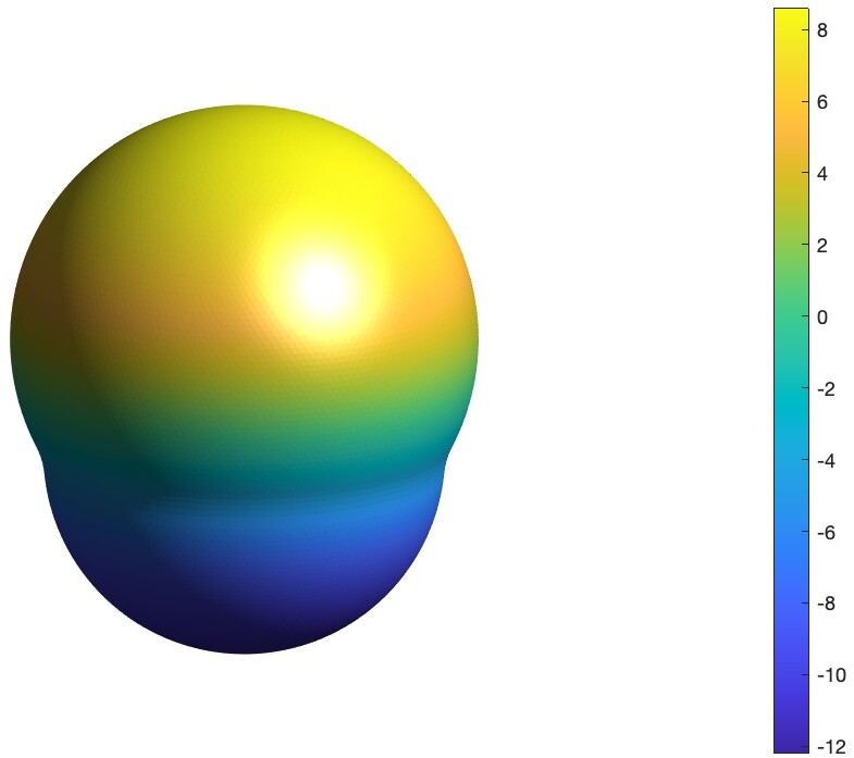
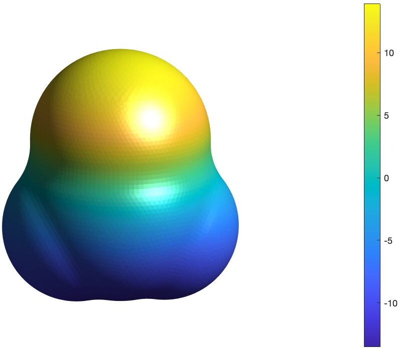
Figure 14: Example 5.6: Reaction potential for hydrogen-fluoride molecule (left) and formaldehyde molecule (right) on $\Omega_{0}$.

Fig. 15 present results for the caffeine molecule, with 24 atoms. Here we use the discretisation parameters $\ell_{\max}=9$, $N_{\mathrm{leb}}=350$, $N=15$, adn $N_{\mathrm{lgl}}=30$. The geometric parameters are set similarly to the previous molecules.

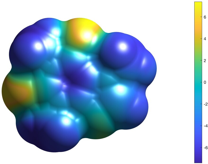
Figure 15: Example 5.6: Reaction potential for caffeine on $\Omega_{0}$.

5.7 Variation of Debye-Hückel Screening Constant

In this example we study the effect of $\kappa$ on the electrostatic solvation energy. We consider the hydrogen fluoride molecule with $r_{0}=0$ Å, and $a=0$ Å; and set the discretisation parameters as $\ell_{\max}=7$, $N_{\mathrm{leb}}=86$, $N=15$, and $N_{\mathrm{lgl}}=30$.

Figure 16: Example 5.7: Electrostatic solvation energy with respect to $\kappa$.

We vary $\kappa$ from $10^{-6}$ to $10^{-4}$. On a continuous level the ddPB-SES model converges to the ddPCM-SES model when $\kappa\rightarrow 0$ (see [43]). We notice similar observations numerically, see Fig. 16. As $\kappa$ decreases the energy becomes constant and converges to a value. We obtain a ddPCM-SES result from [43] using $r_{0}=0$ Å.

6 Summary and Outlook

This paper proposes a new method for solving the Poisson-Boltzmann equation using the domain decomposition paradigm for the solvent-excluded surface.

The original problem defined in $\mathbb{R}^{3}$ is transformed into two-coupled equations described in the bounded solute cavity based on potential theory arguments. An enlarged cavity was defined for each atom encompassing the Stern layer. Then, the Schwarz domain decomposition method was used to solve these two problems by decomposing them into balls. We develop two single-domain solvers for solving the GSP and HSP equations in a unit ball. The GSP solver was a nonlinear solver that used spherical harmonics for angular direction and Legendre polynomials for radial direction. An SES-based continuous dielectric permittivity function and an ion-exclusion function were proposed and were encompassed in the GSP solver. The novelty of the method is that the nonlinearity is incorporated only in the proximity of the molecule whereas in the solvent region the linear model was used. A series of numerical results have been presented to show the performance of the ddPB-SES method.

In the future, we would like to implement this method in our open-source software ddX, [20], to simulate bigger molecules. We would also like to study the nonlinear solver better using Newton’s methods and incorporating acceleration techniques such as dynamic damping and Anderson acceleration.

References

• [1] M. Abramowitz and I.A. Stegun. Handbook of Mathematical Functions: With Formulas, Graphs, and Mathematical Tables. Applied mathematics series. Dover Publications, 1965.
• [2] George B. Arfken, Hans J. Weber, and Frank E. Harris. Mathematical Methods for Physicists. Elsevier, 2013.
• [3] N. A. Baker, D. Sept, S. Joseph, M. J. Holst, and J. A. McCammon. Electrostatics of nanosystems: Application to microtubules and the ribosome. Proceedings of the National Academy of Sciences, 98(18):10037–10041, August 2001.
• [4] Helen M. Berman, John Westbrook, Zukang Feng, Gary Gilliland, T. N. Bhat, Helge Weissig, Ilya N. Shindyalov, and Philip E. Bourne. The Protein Data Bank. Nucleic Acids Research, 28(1):235–242, 01 2000.
• [5] Itamar Borukhov, David Andelman, and Henri Orland. Steric effects in electrolytes: A modified Poisson-Boltzmann equation. Physical Review Letters, 79(3):435–438, July 1997.
• [6] Alexander H. Boschitsch and Marcia O. Fenley. Hybrid boundary element and finite difference method for solving the nonlinear Poisson-Boltzmann equation. Journal of Computational Chemistry, 25(7):935–955, 2004.
• [7] Michal Bosy, Matthew W. Scroggs, Timo Betcke, Erik Burman, and Christopher D. Cooper. Coupling finite and boundary element methods to solve the Poisson-Boltzmann equation for electrostatics in molecular solvation, 2023.
• [8] Eric Cancès, Yvon Maday, and Benjamin Stamm. Domain decomposition for implicit solvation models. The Journal of Chemical Physics, 139(5):054111, August 2013.
• [9] David Leonard Chapman. LI. A contribution to the theory of electrocapillarity. The London, Edinburgh, and Dublin Philosophical Magazine and Journal of Science, 25(148):475–481, April 1913.
• [10] Duan Chen, Zhan Chen, Changjun Chen, Weihua Geng, and Guo-Wei Wei. MIBPB: A software package for electrostatic analysis. Journal of Computational Chemistry, 32(4):756–770, September 2010.
• [11] Long Chen, Michael J. Holst, and Jinchao Xu. The finite element approximation of the nonlinear poisson–boltzmann equation. SIAM Journal on Numerical Analysis, 45(6):2298–2320, January 2007.
• [12] Rochishnu Chowdhury, Raphael Egan, Daniil Bochkov, and Frederic Gibou. Efficient calculation of fully resolved electrostatics around large biomolecules. Journal of Computational Physics, 448:110718, 2022.
• [13] Peter Debye and Erich Hückel. Zur theorie der elektrolyte. i. gefrierpunktserniedrigung und verwandte erscheinungen. Physikalische Zeitschrift, 24(185):305, 1923.
• [14] T. J. Dolinsky, P. Czodrowski, H. Li, J. E. Nielsen, J. H. Jensen, G. Klebe, and N. A. Baker. PDB2pqr: expanding and upgrading automated preparation of biomolecular structures for molecular simulations. Nucleic Acids Research, 35(Web Server):W522–W525, May 2007.
• [15] T. J. Dolinsky, J. E. Nielsen, J. A. McCammon, and N. A. Baker. PDB2pqr: an automated pipeline for the setup of Poisson-Boltzmann electrostatics calculations. 32(Web Server):W665–W667, July 2004.
• [16] Paolo Gatto, Filippo Lipparini, and Benjamin Stamm. Computation of forces arising from the polarizable continuum model within the domain-decomposition paradigm. The Journal of Chemical Physics, 147(22):224108, December 2017.
• [17] Weihua Geng and Robert Krasny. A treecode-accelerated boundary integral Poisson–Boltzmann solver for electrostatics of solvated biomolecules. Journal of Computational Physics, 247:62–78, August 2013.
• [18] M. Gouy. Sur la constitution de la charge électrique à la surface d’un électrolyte. J. Phys. Theor. Appl., 9(1):457–468, 1910.
• [19] Daniel J Haxton. Lebedev discrete variable representation. Journal of Physics B: Atomic, Molecular and Optical Physics, 40(23):4443–4451, November 2007.
• [20] Michael Herbst, Abhinav Jha, Filippo Lipparini, Aleksandr Mikhalev, Michele Nottoli, and Benjamin Stamm. ddx.
• [21] Abhinav Jha, Michele Nottoli, Aleksandr Mikhalev, Chaoyu Quan, and Benjamin Stamm. Linear scaling computation of forces for the domain-decomposition linear poisson–boltzmann method. The Journal of Chemical Physics, 158(10), March 2023.
• [22] Yi Jiang, Yang Xie, Jinyong Ying, Dexuan Xie, and Zeyun Yu. SDPBS web server for calculation of electrostatics of ionic solvated biomolecules. Computational and Mathematical Biophysics, 3(1), November 2015.
• [23] Elizabeth Jurrus, Dave Engel, Keith Star, Kyle Monson, Juan Brandi, Lisa E. Felberg, David H. Brookes, Leighton Wilson, Jiahui Chen, Karina Liles, Minju Chun, Peter Li, David W. Gohara, Todd Dolinsky, Robert Konecny, David R. Koes, Jens Erik Nielsen, Teresa Head-Gordon, Weihua Geng, Robert Krasny, Guo-Wei Wei, Michael J. Holst, J. Andrew McCammon, and Nathan A. Baker. Improvements to the APBS biomolecular solvation software suite. Protein Science, 27(1):112–128, October 2017.
• [24] Johannes Kraus, Svetoslav Nakov, and Sergey Repin. Reliable computer simulation methods for electrostatic biomolecular models based on the poisson–boltzmann equation. Computational Methods in Applied Mathematics, 20(4):643–676, September 2020.
• [25] Gene Lamm. The Poisson-Boltzmann equation. In Reviews in Computational Chemistry, pages 147–365. John Wiley & Sons, Inc., September 2003.
• [26] B. Lee and F.M. Richards. The interpretation of protein structures: Estimation of static accessibility. Journal of Molecular Biology, 55(3):379–IN4, February 1971.
• [27] Lin Li, Chuan Li, Subhra Sarkar, Jie Zhang, Shawn Witham, Zhe Zhang, Lin Wang, Nicholas Smith, Marharyta Petukh, and Emil Alexov. DelPhi: a comprehensive suite for DelPhi software and associated resources. BMC Biophysics, 5(1), May 2012.
• [28] F. Lipparini, B. Stamm, E. Cancès, Y. Maday, and B. Mennucci. Fast domain decomposition algorithm for continuum solvation models: Energy and first derivatives. Journal of Chemical Theory and Computation, 9(8):3637–3648, 2013. PMID: 26584117.
• [29] Filippo Lipparini, Louis Lagardère, Giovanni Scalmani, Benjamin Stamm, Eric Cancès, Yvon Maday, Jean-Philip Piquemal, Michael J. Frisch, and Benedetta Mennucci. Quantum calculations in solution for large to very large molecules: A new linear scaling QM/continuum approach. The Journal of Physical Chemistry Letters, 5(6):953–958, February 2014.
• [30] Filippo Lipparini, Giovanni Scalmani, Louis Lagardère, Benjamin Stamm, Eric Cancès, Yvon Maday, Jean-Philip Piquemal, Michael J. Frisch, and Benedetta Mennucci. Quantum, classical, and hybrid QM/MM calculations in solution: General implementation of the ddCOSMO linear scaling strategy. The Journal of Chemical Physics, 141(18):184108, November 2014.
• [31] Itay Lotan and Teresa Head-Gordon. An analytical electrostatic model for salt screened interactions between multiple proteins. Journal of Chemical Theory and Computation, 2(3):541–555, 2006.
• [32] Benzhuo Lu, Xiaolin Cheng, Jingfang Huang, and J. Andrew McCammon. AFMPB: An adaptive fast multipole poisson–boltzmann solver for calculating electrostatics in biomolecular systems. Computer Physics Communications, 181(6):1150–1160, June 2010.
• [33] Benzhuo Lu, Yongcheng Zhou, Michael Holst, and J Mccammon. Recent progress in numerical methods for the Poisson-Boltzmann equation in biophysical applications. Communications in Computational Physics, 37060:973–1009, 04 2008.
• [34] Jeffry D. Madura, James M. Briggs, Rebecca C. Wade, Malcolm E. Davis, Brock A. Luty, Andrew Ilin, Jan Antosiewicz, Michael K. Gilson, Babak Bagheri, L.Ridgway Scott, and J.Andrew McCammon. Electrostatics and diffusion of molecules in solution: simulations with the university of houston brownian dynamics program. Computer Physics Communications, 91(1-3):57–95, September 1995.
• [35] A. Mikhalev, M. Nottoli, and B. Stamm. Linearly scaling computation of ddPCM solvation energy and forces using the fast multipole method. The Journal of Chemical Physics, 157(11), September 2022.
• [36] Mohammad Mirzadeh, Maxime Theillard, and Frédéric Gibou. A second-order discretization of the nonlinear poisson–boltzmann equation over irregular geometries using non-graded adaptive cartesian grids. Journal of Computational Physics, 230(5):2125–2140, March 2011.
• [37] Mohammad Mirzadeh, Maxime Theillard, Asdís Helgadöttir, David Boy, and Frédéric Gibou. An adaptive, finite difference solver for the nonlinear Poisson-Boltzmann equation with applications to biomolecular computations. Communications in Computational Physics, 13(1):150–173, January 2013.
• [38] Svetoslav Nakov, Ekaterina Sobakinskaya, Thomas Renger, and Johannes Kraus. ARGOS: An adaptive refinement goal-oriented solver for the linearized poisson–boltzmann equation. Journal of Computational Chemistry, 42(26):1832–1860, July 2021.
• [39] Michele Nottoli, Benjamin Stamm, Giovanni Scalmani, and Filippo Lipparini. Quantum Calculations in Solution of Energies, Structures, and Properties with a Domain Decomposition Polarizable Continuum Model. J. Chem. Theory Comput., 15(11):6061–6073, November 2019.
• [40] Modesto Orozco and F Javier Luque. Theoretical methods for the description of the solvent effect in biomolecular systems. Chemical Reviews, 100(11):4187–4226, 2000.
• [41] Seymour V. Parter. On the legendre–gauss–lobatto points and weights. Journal of Scientific Computing, 14(4):347–355, 1999.
• [42] C. Quan and B. Stamm. Mathematical analysis and calculation of molecular surfaces. J. Comput. Phys., 322:760–782, 2016.
• [43] C. Quan, B. Stamm, and Y. Maday. A domain decomposition method for the polarizable continuum model based on the solvent excluded surface. Math. Models Methods Appl. Sci., 28(7):1233–1266, 2018.
• [44] C. Quan, B. Stamm, and Y. Maday. A domain decomposition method for the Poisson-Boltzmann solvation models. SIAM J. Sci. Comput., 41(2):B320–B350, 2019.
• [45] Alfio Quarteroni and Alberto Valli. Domain Decomposition Methods for Partial Differential Equations. Oxford University Press, 1999.
• [46] Arnold Reusken and Benjamin Stamm. Analysis of the Schwarz domain decomposition method for the conductor-like screening continuum model. SIAM J. Numer. Anal., 59(2):769–796, 2021.
• [47] Frederic M Richards. Areas, volumes, packing, and protein structure. Annual review of biophysics and bioengineering, 6(1):151–176, 1977.
• [48] Stefan Ringe, Harald Oberhofer, Christoph Hille, Sebastian Matera, and Karsten Reuter. Function-space-based solution scheme for the size-modified poisson–boltzmann equation in full-potential DFT. Journal of Chemical Theory and Computation, 12(8):4052–4066, July 2016.
• [49] Benoıt Roux and Thomas Simonson. Implicit solvent models. Biophysical chemistry, 78(1-2):1–20, 1999.
• [50] Stefan A. Sauter and Christoph Schwab. Boundary Element Methods. Springer Berlin Heidelberg, 2011.
• [51] Benjamin Stamm, Eric Cancès, Filippo Lipparini, and Yvon Maday. A new discretization for the polarizable continuum model within the domain decomposition paradigm. The Journal of Chemical Physics, 144(5):054101, February 2016.
• [52] Christopher J. Stein, John M. Herbert, and Martin Head-Gordon. The poisson–boltzmann model for implicit solvation of electrolyte solutions: Quantum chemical implementation and assessment via sechenov coefficients. The Journal of Chemical Physics, 151(22):224111, December 2019.
• [53] Otto Stern. Zur theorie der elektrolytischen doppelschicht. 1924.
• [54] Jacopo Tomasi, Benedetta Mennucci, and Roberto Cammi. Quantum mechanical continuum solvation models. Chemical Reviews, 105(8):2999–3094, July 2005.
• [55] Jacopo Tomasi and Maurizio Persico. Molecular interactions in solution: an overview of methods based on continuous distributions of the solvent. Chemical Reviews, 94(7):2027–2094, 1994.
• [56] Leighton Wilson, Weihua Geng, and Robert Krasny. TABI-PB 2.0: An improved version of the treecode-accelerated boundary integral Poisson-Boltzmann solver. The Journal of Physical Chemistry B, 126(37):7104–7113, September 2022.
• [57] Dexuan Xie. New solution decomposition and minimization schemes for poisson–boltzmann equation in calculation of biomolecular electrostatics. Journal of Computational Physics, 275:294–309, October 2014.
• [58] Yang Xie, Jinyong Ying, and Dexuan Xie. SMPBS: Web server for computing biomolecular electrostatics using finite element solvers of size modified Poisson-Boltzmann equation. Journal of Computational Chemistry, 38(8):541–552, January 2017.
• [59] Eng-Hui Yap and Teresa Head-Gordon. New and efficient Poisson-Boltzmann solver for interaction of multiple proteins. Journal of Chemical Theory and Computation, 6(7):2214–2224, 2010.
• [60] Eng-Hui Yap and Teresa Head-Gordon. Calculating the bimolecular rate of protein–protein association with interacting crowders. Journal of Chemical Theory and Computation, 9(5):2481–2489, 2013.
• [61] Jinyong Ying and Dexuan Xie. A new finite element and finite difference hybrid method for computing electrostatics of ionic solvated biomolecule. Journal of Computational Physics, 298:636–651, October 2015.
• [62] Bo Zhang, Bo Peng, Jingfang Huang, Nikos P. Pitsianis, Xiaobai Sun, and Benzhuo Lu. Parallel AFMPB solver with automatic surface meshing for calculation of molecular solvation free energy. Computer Physics Communications, 190:173–181, May 2015.