On the Local Quadratic Stability of T-S Fuzzy Systems in the Vicinity of the Origin

Abstract

The main goal of this paper is to introduce new local stability conditions for continuous-time Takagi-Sugeno (T-S) fuzzy systems. These stability conditions are based on linear matrix inequalities (LMIs) in combination with quadratic Lyapunov functions. Moreover, they integrate information on the membership functions at the origin and effectively leverage the linear structure of the underlying nonlinear system in the vicinity of the origin. As a result, the proposed conditions are proved to be less conservative compared to existing methods using fuzzy Lyapunov functions. Moreover, we establish that the proposed methods offer necessary and sufficient conditions for the local exponential stability of T-S fuzzy systems. The paper also includes discussions on the inherent limitations associated with fuzzy Lyapunov approaches. To demonstrate the theoretical results, we provide comprehensive examples that elucidate the core concepts and validate the efficacy of the proposed conditions.

I Introduction

Over the past several decades, Takagi–Sugeno (T–S) fuzzy systems have gained prominence as effective tools for modeling nonlinear systems [1]. These systems are characterized by a convex combination of linear subsystems, each weighted by nonlinear membership functions (MFs) [2]. Particularly within the framework of Lyapunov theory, T–S fuzzy systems offer a systematic approach for leveraging linear system theories in the stability analysis and control design of nonlinear systems. Moreover, these systems facilitate the formulation of problems based on convex linear matrix inequality (LMI) optimization procedures, which are readily solvable through standard convex optimization techniques [3]. Due to these advantages, there has been a surge of interest in the stability analysis and control design of T–S fuzzy systems in recent years [4].

Despite these advantages, T–S fuzzy model-based methods are often subject to a considerable degree of conservatism, which can be attributed to multiple sources: 1) The discrepancy between the infinite-dimensional parameterized matrix inequalities, which naturally arise in Lyapunov inequalities, and the numerically tractable finite-dimensional LMI problems introduces significant conservatism; 2) The constrained architectures of the Lyapunov functions and control laws can also be a source of conservatism; 3) Attempts to ensure stability across an overly expansive region of the state-space can lead to conservatism, particularly when the underlying nonlinear system only exhibits stability within a small region around the origin.

To reduce the conservatism, extensive research efforts have been undertaken. These efforts can be broadly classified into three primary categories:

1. Relaxation of Parameterized LMIs: Techniques for relaxing parameterized LMIs have also been developed. These include slack variable methods [5, 6], multidimensional convex summation techniques based on Polya’s theorem [7, 8], as well as methods that leverage the structural information of membership functions [9, 10, 11] to name just a few.

2. Generalization of Lyapunov Functions and Control Laws: Various extensions to traditional Lyapunov functions have been proposed, including piecewise Lyapunov functions [12, 13, 14], fuzzy Lyapunov functions (FLFs) [15, 16, 17, 18, 19, 20, 21, 22, 19, 23], line-integral Lyapunov functions [24], polynomial Lyapunov functions [25, 26, 27, 28], and augmented FLFs [29, 30] to name just a few.

3. Local Stability Approaches: Some studies focus on estimating the domain of attraction through local stability analysis [31, 28, 32, 33, 22]. By assessing stability within a localized region, these approaches aim to reduce conservatism by balancing the trade-off between the volume of the domain of attraction and the degree of conservatism.

The primary aim of this paper is to introduce new local stability conditions for continuous-time T-S fuzzy systems by building upon the common quadratic Lyapunov function (QLF) approach [34]. While the QLF method is straightforward and widely used, it is known to introduce considerable conservatism. This conservatism is primarily due to the common Lyapunov matrix that should be found across all subsystems of the underlying fuzzy system.

In addressing these challenges, this paper demonstrates that the limitations associated with the common QLF approach can be mitigated. This is achieved by incorporating information about the membership functions at the origin into the quadratic stability conditions and by effectively leveraging the linear structure of the underlying nonlinear system in proximity to the origin. Consequently, the proposed quadratic stability conditions are theoretically proven to be less conservative than existing FLF methods in the literature.

The main contributions of this paper can be summarized as follows: 1) We develop several LMI stability conditions based on the QLF. Both theoretical and numerical evidences are provided to demonstrate that these quadratic stability conditions are less conservative compared to those based on FLFs in existing literature; 2) We rigorously establish that the proposed methods yield necessary and sufficient conditions for ensuring the local exponential stability of T-S fuzzy systems; 3) We identify and discuss the inherent limitations associated with both the QLF and FLF approaches. To substantiate these theoretical insights, comprehensive examples are provided to clarify the core concepts underpinning our contributions; 4) We demonstrate that the proposed QLF approach can be synergistically integrated with FLF methods to produce compounded effects, thereby reducing conservatism of existing stability conditions.

The organization of this paper is as follows: Section II introduces preliminary definitions, reviews existing quadratic and FLF approaches, and provides initial discussions to set the stage for the paper. Section III contains the main results, detailing the proposed stability conditions along with associated examples and discussions to validate the theoretical contributions. Section IV offers a comprehensive analysis, including discussions on the reduced conservatism of the proposed conditions, converse theorems, and the fundamental limitations of various approaches. This section also includes relevant examples to support the analysis. Section V integrates the two primary methods discussed in this paper—the FLF and QLF approaches—and analyzes their combined effects. Finally, Section VI concludes the paper, offering remarks on potential topics for future research.

II Preliminaries

II-A Notation

The adopted notation is as follows. ${\mathbb{R}}$: sets of real numbers; $A^{T}$: transpose of matrix $A$; $A\succ 0$ ($A\prec 0$, $A\succeq 0$, and $A\preceq 0$, respectively): symmetric positive definite (negative definite, positive semi-definite, and negative semi-definite, respectively) matrix $A$; $I_{n}$ and $I$: $n\times n$ identity matrix and identity matrix of appropriate dimensions, respectively; $0$: zero vector of appropriate dimensions; $\lambda_{\min}(A)$ and $\lambda_{\max}(A)$: minimum and maximum eigenvalues of symmetric matrix $A$, respectively.

II-B Takagi–Sugeno (T–S) fuzzy system

Consider the continuous-time nonlinear system

$$\dot{x}(t)=f(x(t)),$$ (1)

where $t\geq 0$ is the time, $x(t):=\begin{bmatrix}x_{1}(t)&\cdots&x_{n}(t)\\ \end{bmatrix}^{T}\in{\mathbb{R}}^{n}$ is the state, $f:{\mathbb{R}}^{n}\to{\mathbb{R}}^{n}$ is a nonlinear function such that $f(0)=0$, i.e., the origin is an equilibrium point of (1). By the sector nonlinearity approach [2], one can obtain the following T–S fuzzy system representation of the nonlinear system (1) in the subset ${\cal X}$ of the state-space ${\mathbb{R}}^{n}$:

$$\dot{x}(t)=\sum_{i=1}^{r}{{\alpha_{i}}(x(t)){A_{i}}x(t)}=:A(\alpha(t))x(t),\quad\forall x(t)\in{\cal X}$$ (2)

where $A_{i}\in{\mathbb{R}}^{n\times n},i\in\{1,2,\ldots,r\}$ are subsystem matrices, $i\in{\cal I}_{r}:=\{1,\,2,\ldots,\,r\}$ is the rule number, $\alpha_{i}:\,{\mathbb{R}}^{n}\to[0,\,1]$ is the membership function (MF) for each rule, and the vector of the MFs

$$\alpha(x):=\left[{\begin{array}[]{*{20}{c}}{{\alpha_{1}}(x)}\\ {{\alpha_{2}}(x)}\\ \vdots\\ {{\alpha_{r}}(x)}\end{array}}\right]\in{\mathbb{R}}^{r}$$

lies in the unit simplex

$${\Lambda_{r}}:=\left\{{\begin{array}[]{*{20}{c}}{\alpha\in{\mathbb{R}}^{r}:\sum\limits_{i=1}^{r}{{\alpha_{i}}}=1,0\leq{\alpha_{i}}\leq 1,i\in{\cal I}_{r}}\end{array}}\right\}.$$

In addition, ${\cal X}\in{\mathbb{R}}^{n}$ is a subset of the state-space ${\mathbb{R}}^{n}$ including the origin $0\in{\cal X}$ and satisfies

$${\cal X}\subseteq\left\{{x\in{\mathbb{R}}^{n}:f(x)=\sum_{i=1}^{r}{{\alpha_{i}}(x)A_{i}x}}\right\}$$ (3)

In other words, ${\cal X}$ is a modelling region where the T–S fuzzy model is defined. In this paper, we assume that ${\cal X}$ is compact.

II-C Quadratic stability

Let us consider the quadratic Lyapunov function (QLF) candidate $V(x)=x^{T}Px$, where $P=P^{T}\succ 0$ is some matrix. Its time-derivative along the solution of (1) is given as

$$\dot{V}(x(t))=x{(t)^{T}}\sum_{i=1}^{r}{{\alpha_{i}}(x(t))(A_{i}^{T}P+P{A_{i}})x(t)}$$

Using Lyapunov direct method [1], the corresponding stability condition is given below.

Lemma 1 ([2, Theorem 5]).

Suppose that there exists a symmetric matrix $P=P^{T}\in{\mathbb{R}}^{n\times n}$ such that the following LMIs hold:

$$P\succ 0,\quad A_{i}^{T}P+P{A_{i}}\prec 0,\quad i\in{\cal I}_{r}.$$

Then, the fuzzy system (2) is locally asymptotically stable.

When the LMIs are feasible, then the system is locally asymptotically stable, and the domain of attraction (DA) [1] is given by any Lyapunov sublevel sets defined by

$${L_{V}}(c):=\{x\in{\mathbb{R}}^{n}:V(x)\leq c\}\subseteq{\cal X}$$

with any $c>0$ such that ${L_{V}}(c)\subseteq{\cal X}$. The largest DA is ${L_{V}}(c^{*})$ with ${c^{*}}:=\max\{c>0:{L_{V}}(c)\subseteq{\cal X}\}$. While the LMI condition offers simplicity, a key drawback of the quadratic stability approach is its inherent conservatism. This conservatism primarily stems from the requirement for a common Lyapunov matrix $P$, which should satisfy the Lyapunov inequality across all subsystems of the fuzzy system. As an alternative, the fuzzy Lyapunov function (FLF) can be employed.

II-D Fuzzy Lyapunov stability

Let us consider the Lyapunov function candidate

$$V(x)={x^{T}}\left({\sum_{i=1}^{r}{{\alpha_{i}}(x)P_{i}}}\right)x=:{x^{T}}P(\alpha(x))x,$$

which is called a fuzzy Lyapunov function (FLF), where $P_{i}=P_{i}^{T}\succ 0,i\in{\cal I}_{r}$. Taking its time-derivative along the trajectory of (2) leads to

$$\dot{V}(x(t))= x{(t)^{T}}\left[{\sum\limits_{i=1}^{r}{\sum\limits_{j=1}^{r}{{\alpha_{i}}(x(t)){\alpha_{j}}(x(t))(A_{i}^{T}{P_{j}}+{P_{j}}{A_{i}})}}}\right.$$

$$\left.{\sum\limits_{k=1}^{r}{{{\dot{\alpha}}_{k}}(x(t)){P_{k}}}}\right]x(t).$$

It is important to note that the use of the FLF presupposes that the MFs are differentiable, an assumption that does not universally hold. Therefore, when employing the FLF, we implicitly assume the differentiability of the MFs. A challenge that emerges in this context is that the stability condition depends on the derivatives of the MFs, which are not readily amenable to convexification. To circumvent this issue, [15] proposed incorporating a bound on the derivatives of the MFs, $|{\nabla_{x}}{\alpha_{i}}(x)A(\alpha(x))x|\leq{\varphi_{i}},i\in{\cal I}_{r},x\in{\cal X}$. Building on this bound, a subsequent LMI-based stability condition has been introduced.

Lemma 2 ([15, Theorem 1]).

Suppose that the MFs are differentiable. Moreover, suppose that there exist constants $\varphi_{k}>0,k\in{\cal I}_{r}$, symmetric matrices $P_{i}=P_{i}^{T}\in{\mathbb{R}}^{n\times n},i\in{\cal I}_{r}$ such that the following LMIs hold:

$$P_{i}\succ 0,\quad i\in{\cal I}_{r}$$

$$\sum\limits_{k=1}^{r}{{\varphi_{k}}{P_{k}}}+\frac{1}{2}\left({A_{i}^{T}{P_{j}}+{P_{j}}{A_{i}}+A_{j}^{T}{P_{i}}+{P_{i}}{A_{j}}}\right)\prec 0,$$

$$\forall(i,j)\in{\cal I}_{r}\times{\cal I}_{r},\quad i\leq j.$$

Then, the fuzzy system (2) is locally asymptotically stable.

In the Fuzzy Lyapunov Function (FLF) approach, the imposed bounds $|{\nabla_{x}}{\alpha_{i}}{(x)^{T}}A(\alpha(x))x|\leq{\varphi_{i}},i\in{\cal I}_{r}$ imply that the matrix $A(\alpha(x))$ varies at a sufficiently slow rate. This constraint effectively limits the rate of change of the system’s dynamics as represented by $A(\alpha(x))$, thereby facilitating the application of the FLF method for stability analysis. To proceed, let us define the set

$$\Omega(\varphi):=\{x\in{\cal X}:|{\nabla_{x}}{\alpha_{i}}{(x)^{T}}A(\alpha(x))x|\leq{\varphi_{i}},i\in{\cal I}_{r}\}$$

where $\varphi:={\left[{\begin{array}[]{*{20}{c}}{{\varphi_{1}}}&{{\varphi_{2}}}&\cdots&{{\varphi_{r}}}\end{array}}\right]^{T}}$. Clearly, this set is a subset of $\cal X$ such that the derivatives of the MFs are bounded within certain intervals. If the LMIs in Lemma 2 are feasible, then we have

$$V(x)>0,\quad\forall x\in{\cal X}\backslash\{0\},$$

$${\nabla_{x}}V{(x)^{T}}A(\alpha(x))x<0,\quad\forall x\in\Omega(\varphi)\backslash\{0\}.$$

Therefore, from the Lyapunov direct method [1], any Lyapunov sublevelset

$${L_{V}}(c):=\{x\in{\mathbb{R}}^{n}:V(x)\leq c\},$$

with some $c>0$ such that ${L_{V}}(c)\subseteq\Omega(\varphi)$ is a domain of attraction (DA). A fundamental question that naturally arises in this context is whether the set $\Omega(\varphi)$ includes a neighborhood of the origin, i.e., a ball centered at the origin. The significance of this question is directly tied to the practical utility of the conditions elaborated upon in this paper; if $\Omega(\varphi)$ does not include a neighborhood of the origin, then the proposed conditions would be useless for stability analysis around that point. Fortunately, the answer to this question is positive under certain mild assumptions.

Theorem 1.

Suppose that the MFs $\alpha(x)$ are continuously differentiable on $\cal X$. Then, 1) the derivatives of the MFs are bounded in $\cal X$, 2) we have $\lim_{x\to 0_{n}}|{\nabla_{x}}{\alpha_{i}}(x)A(\alpha(x))x|=0,\forall i\in{\cal I}_{r}$, and 3) there exists a ball ${\cal B}(\varepsilon):=\{x\in{\mathbb{R}}^{n}:{\left\|x\right\|_{2}}\leq\varepsilon\}$ of radius $\varepsilon>0$ centered at the origin such that ${\cal B}(\varepsilon)\subseteq\Omega(\varphi)$.

The proof is given in Appendix A. Theorem 1 indicates that for the set $\Omega(\varphi)$ to include a neighborhood of the origin, it is not sufficient for the MFs to merely be differentiable; their derivatives must also exhibit continuity. To elucidate this point, we present an example featuring MFs that are differentiable over the set $\cal X$, but whose derivatives lack continuity and show its impact on the stability conditions.

Example 1.

Let us consider the MFs

$${\alpha_{1}}(x)=\left\{{\begin{array}[]{*{20}{c}}{0,\quad{\rm{if}}{\mkern 1.0mu}{\mkern 1.0mu}x=0}\\ {{x^{2}}\left({\frac{1}{2}\sin\left({\frac{\pi}{{2x}}}\right)+\frac{1}{2}}\right),\quad{\rm{if}}{\mkern 1.0mu}{\mkern 1.0mu}x\in[-1,1]\backslash\{0\}}\end{array}}\right.$$

$${\alpha_{2}}(x)=1-{\alpha_{1}}(x)$$

with ${\cal X}=[-1,1]$. The functions ${\alpha_{1}}$ and ${\alpha_{2}}$ are continuous on $\cal X$. Its derivative in $x\in[-1,1]$ is given by

$$\frac{d}{{dx}}{\alpha_{1}}(x)=\left\{{\begin{array}[]{*{20}{c}}{0,\quad{\rm{if}}\quad x=0}\\ \begin{array}[]{l}2x\left({\frac{1}{2}\sin\left({\frac{\pi}{{2x}}}\right)+\frac{1}{2}}\right)-\frac{\pi}{2}\cos\left({\frac{\pi}{{2x}}}\right),\\ {\rm{if}}\quad x\in[-1,1]\backslash\{0\}\end{array}\end{array}}\right.$$

which is discontinuous because it oscillates as $x\to 0$. Therefore, $\lim_{x\to 0}|{\nabla_{x}}{\alpha_{i}}(x)A(\alpha(x))x|,\forall i\in{\cal I}_{r}$ do not exist. As a consequence, although $\Omega(\varphi)$ contains the origin, it does not contain any ball centered at the origin.

In [16], an improved (less conservative) LMI condition has been proposed using the null effect

$$\sum\limits_{k=1}^{r}{{{\dot{\alpha}}_{k}}(x(t))}=0.$$ (4)

Using this property, one can add the slack term $\sum_{k=1}^{r}{{{\dot{\alpha}}_{k}}(x(t))}M=0$ with any slack matrix variable $M$. For convenience and completeness of the presentation, the condition is formally introduced below.

Lemma 3 ([16, Theorem 6]).

Suppose that the MFs are continuously differentiable. Moreover, suppose that there exist constants $\varphi_{k}>0,k\in{\cal I}_{r}$, symmetric matrices $P_{i}=P_{i}^{T}\in{\mathbb{R}}^{n\times n},i\in{\cal I}_{r}$ and $M=M^{T}\in{\mathbb{R}}^{n\times n}$ such that the following LMIs hold:

$$P_{i}\succ 0,\quad P_{i}+M\succeq 0,\quad i\in{\cal I}_{r}$$

$$\sum\limits_{k=1}^{r}{{\varphi_{k}}{(P_{k}+M)}}+\frac{1}{2}\left({A_{i}^{T}{P_{j}}+{P_{j}}{A_{i}}+A_{j}^{T}{P_{i}}+{P_{i}}{A_{j}}}\right)\prec 0,$$

$$\forall(i,j)\in{\cal I}_{r}\times{\cal I}_{r},\quad i\leq j$$ (5)

Then, the fuzzy system (2) is locally asymptotically stable.

As before, if the LMI condition in Lemma 3 is feasible, then any Lyapunov sublevelset ${L_{V}}(c)$ with some $c>0$ such that ${L_{V}}(c)\subseteq\Omega(\varphi)$ is a DA. As $\varphi_{i}$ approaches zero for $i\in{\cal I}_{r}$, the associated LMI condition in Lemma 3 become less conservative. However, this reduction in conservatism comes at a cost: the set $\Omega(\varphi)$ contracts towards the origin, leading to a corresponding reduction in the DA. This situation shows a trade-off between the level of conservatism in the stability conditions and the volume of the DA. In essence, achieving less conservative conditions results in a more restricted DA. A natural question arising here is if the conservatism can be completely eliminated as $\varphi_{i}$ approaches zero for $i\in{\cal I}_{r}$. The answer to this question is, in fact, negative, as demonstrated by the subsequent result.

Theorem 2 (Fundamental limitation).

Consider a nonlinear function (1) that is locally exponentially stable around the origin and the corresponding fuzzy system (2). Suppose that its MFs are continuously differentiable on $\cal X$. Then, corresponding the LMI condition of Lemma 3 may be infeasible for any $\varphi_{i},i\in{\cal I}_{r}$.

The proof is given in Appendix B. Theorem 2 establishes that the FLF approach contains an intrinsic conservatism that cannot be fully mitigated. Before concluding this section, we note two primary limitations of the FLF approach: First, its applicability is restricted to cases where the MFs are continuously differentiable. Second, as established in Theorem 2, the approach exhibits inherent conservatism that cannot be fully eliminated. These limitations serve to delineate the scope and efficacy of the FLF approach in stability analysis. In contrast, the local QLF approaches proposed in the subsequent sections can overcome these disadvantages inherent to the FLF methods.

III Main results

In this section, a new idea is proposed based on QLFs. First of all, let us rewrite the system (2) into

$$\dot{x}(t)= A(\alpha(t))x(t)$$

$$= \sum\limits_{i=1}^{r}{{\alpha_{i}}(x(t)){A_{i}}x(t)}$$

$$= \sum\limits_{i=1}^{r}{({\alpha_{i}}(x(t))-{\alpha_{i}}(0)){A_{i}}x(t)}+\underbrace{\sum\limits_{i=1}^{r}{{\alpha_{i}}(0){A_{i}}}}_{=:{A_{0}}}x(t)$$

$$= \sum\limits_{i=1}^{r}{({\alpha_{i}}(x(t))-{\alpha_{i}}(0)){A_{i}}x(t)}+{A_{0}}x(t),$$

which can be seen as a decomposition of the original system, $\dot{x}(t)=A(\alpha(x(t)))x(t)$, into the sum of the nominal linear system ${A_{0}}x(t)$ and the perturbed term $\sum_{i=1}^{r}{({\alpha_{i}}(x(t))-{\alpha_{i}}(0)){A_{i}}x(t)}$. The error term is expressed in terms of the difference between the MF ${\alpha_{i}}(x(t))$ at the current state $x(t)$ and the MF at the origin ${\alpha_{i}}(0)$.

Consequently, it is reasonable to conjecture that as $x(t)\to 0$, the error term diminishes, leaving only the nominal linear term. In this context, the nominal system can be considered as the limiting case of the fuzzy system described by (2) as the state $x(t)$ approaches the origin $0$. If the MFs are continuous over the set $\cal X$, then as $x(t)\to 0$, the difference $|\alpha_{i}(x(t))-\alpha_{i}(0)|$ converges to zero for all $i\in{\cal I}_{r}$. Consequently, the error term $\sum_{i=1}^{r}{({\alpha_{i}}(x(t))-{\alpha_{i}}(0)){A_{i}}x(t)}$ also tends toward zero.

Lemma 4.

Suppose that the MFs are continuous on $\cal X$. Then, $\lim_{x\to 0}|{\alpha_{i}}(x)-{\alpha_{i}}(0)|=0,\forall i\in{\cal I}_{r}$.

This result is a direct consequence of the continuity of the MFs. The following example shows the consequence when the continuity assumption is not met.

Example 2.

Let us consider the MFs

$${\alpha_{1}}(x)= \left\{{\begin{array}[]{*{20}{c}}{\frac{1}{2},\quad{\rm{if}}{\mkern 1.0mu}{\mkern 1.0mu}\,\,x=0}\\ {\frac{1}{2}\sin\left({\frac{\pi}{{2x}}}\right)+\frac{1}{2},\quad{\rm{if}}{\mkern 1.0mu}{\mkern 1.0mu}\,\,x\in[-1,1]\backslash\{0\}}\end{array}}\right.$$

$${\alpha_{2}}(x)= 1-{\alpha_{1}}(x)$$

with ${\cal X}=[-1,1]$. The functions ${\alpha_{1}}$ is discontinuous at $x=0$. The difference is given by

$$|{\alpha_{1}}(x)-{\alpha_{1}}(0)|={\alpha_{1}}(x)=\frac{1}{2}\sin\left({\frac{\pi}{{2x}}}\right),\quad x\in[-1,1]\backslash\{0\},$$

which does not converge to $0$ as $x\to 0$. Therefore, ${\cal H}(b)$ contains the origin, but does not contain any ball centered at the origin.

In this section, we consider the QLF candidate $V(x)=x^{T}Px$, where $P\succ 0$. Its time-derivative along the solution of (2) is given as

$$\dot{V}(x(t))= \sum\limits_{i=1}^{r}{({\alpha_{i}}(x(t))-{\alpha_{i}}(0))x{{(t)}^{T}}(A_{i}^{T}P+P{A_{i}})}x(t)$$

$$+x{(t)^{T}}(A_{0}^{T}P+P{A_{0}})x(t)$$ (6)

By Lyapunov theorem [1], the asymptotic stability is guaranteed if $V(x(t))>0,\forall x(t)\in{\cal X}\backslash\{0\}$ and $\dot{V}(x(t))<0,\forall x(t)\in{\cal X}\backslash\{0\}$, which is guaranteed if the following Lyapunov matrix inequalities hold:

$$P\succ 0,$$

$$\sum\limits_{i=1}^{r}{({\alpha_{i}}(x))-{\alpha_{i}}(0))(A_{i}^{T}P+P{A_{i}})}+A_{0}^{T}P+P{A_{0}}\prec 0$$ (7)

In what follows, we will derive three sufficient LMI conditions based on (7). The proposed conditions can be categorized into two classes depending on how to treat the difference term $({\alpha_{i}}(x))-{\alpha_{i}}(0))$, which are summarized as follows:

1. Polytopic bound (hyper rectangle bound):

   $$|{\alpha_{i}}(x))-{\alpha_{i}}(0)|\leq{b_{i}},\quad i\in{\cal I}_{r}$$ (8)

   where $b_{i}\in[0,1],i\in{\cal I}_{r}$. Equivalently, it can be written as

   $$\left[{\begin{array}[]{*{20}{c}}{{\alpha_{1}}(x)-{\alpha_{1}}(0)}\\ \vdots\\ {{\alpha_{r}}(x)-{\alpha_{r}}(0)}\end{array}}\right]=: \alpha(x)-\alpha(0)\in{\cal D}(b),$$

   where ${\cal D}(b)$ is a hyper rectangle defined as

   $${\cal D}(b):=\{\delta\in{\mathbb{R}}^{r}:|{\delta_{i}}|\leq b_{i},i\in{\cal I}_{r}\}.$$ (9)

2. Ball bound: for any $\eta>0$,

   $$\sum_{i=1}^{r}{{{({\alpha_{i}}(z)-{\alpha_{i}}(0))}^{2}}}\leq\eta.$$

Another important property we will use is the following null effect:

$$\sum_{i=1}^{r}{({\alpha_{i}}(x(t))-{\alpha_{i}}(0))}=0$$ (10)

which is similar to the null effect of the derivatives of the MFs in (4). Such a geometric information can be used in the sequel in order to reduce conservatism of LMI stability conditions.

III-A Local quadratic stability based on the polytopic bound

In this subsection, we introduce two LMI conditions. The first LMI condition employs all vertices of the polytopic bound as described in (8). The second LMI condition utilizes an over-bounding technique, akin to the method outlined in Lemma 3. We commence with the first setting. Specifically, by evaluating the condition at all vertices of the polytope, we can derive the following finite-dimensional LMI condition.

Theorem 3 (Local quadratic stability I).

Suppose that the MFs are continuous. Moreover, suppose that there exist constants $b_{i}\in[0,1],i\in{\cal I}_{r}$, symmetric matrices $P=P^{T}\in{\mathbb{R}}^{n\times n}$ and $M=M^{T}\in{\mathbb{R}}^{n\times n}$ such that the following LMIs hold:

$$P\succ 0,$$

$$A_{0}^{T}P+P{A_{0}}+\sum\limits_{i=1}^{r}{{\delta_{i}}(A_{i}^{T}P+P{A_{i}}+M)}\prec 0,$$

$$({\delta_{1}},{\delta_{2}},\ldots,{\delta_{r}})\in\{-{b_{1}},{b_{1}}\}\times\{-{b_{2}},{b_{2}}\}\times\cdots\times\{-{b_{r}},{b_{r}}\}$$ (11)

Then, the fuzzy system (2) is locally asymptotically stable.

The proof is given in Appendix C. A notable difference between the condition in Theorem 3 and those in fuzzy Lypaunov approaches is that the condition in Theorem 3 uses information on the MFs, i.e., $\alpha(0)$, while the conditions derived from fuzzy Lypaunov approaches (e.g., Lemma 2, Lemma 3) do not depend on the MFs. If the condition in Theorem 3 is feasible, then it implies that there exists $P=P^{T}\succ 0$ such that

$$A{(\alpha(x))^{T}}P+PA(\alpha(x))\prec 0,\quad\forall x\in{\cal H}(b),$$

where

$${\cal H}(b):=\{x\in{\cal X}:|{\alpha_{i}}(x)-{\alpha_{i}}(0)|\leq{b_{i}},i\in{\cal I}_{r}\},$$

$b:={\left[{\begin{array}[]{*{20}{c}}{{b_{1}}}&{{b_{2}}}&\cdots&{{b_{r}}}\end{array}}\right]^{T}}\in{\mathbb{R}}^{r}$, and ${b_{i}}\in[0,1]$ for all $i\in{\cal I}_{r}$, which corresponds to $\Omega(\varphi)$ in the FLF approach, while has several differences. Moreover any Lyapunov sublevelset such that ${L_{V}}(c)\subseteq{\cal H}(b)$ with some $c>0$ is a DA. Similar to the FLF methods, the proposed conditions are only useful when ${\cal H}(b)$ contains some neighborhood of the origin. In the sequel, we prove that ${\cal H}(b)$ includes neighborhoods of the origin under the continuity assumption.

Similar to the constraints associated with FLFs, the applicability of the proposed conditions hinges on whether the set ${\cal H}(b)$ includes a neighborhood of the origin. In what follows, we establish that ${\cal H}(b)$ does, in fact, encompass neighborhoods of the origin, provided that the continuity assumption holds. This validation serves to affirm the applicability and effectiveness of the proposed stability conditions.

Theorem 4.

Suppose that the MFs are continuous on $\cal X$. Then, there exists a ball ${\cal B}(c)$ with some $c>0$ such that ${\cal B}(c)\subseteq{\cal H}(b)$ for any $b_{i}\in[0,1],i\in{\cal I}_{r}$.

Proof.

From the definition of continuous functions, for any given $b_{i}\in[0,1],i\in{\cal I}_{r}$, we can find a ball ${\cal B}(c_{i})$ with some $c_{i}>0$ such that $|{\alpha_{i}}(x)-{\alpha_{i}}(0)|\leq{b_{i}},\forall x\in{\cal B}({c_{i}}),i\in{\cal I}_{r}$. Then, letting $c={\min_{i\in{\cal I}_{r}}}{c_{i}}$ leads to ${\cal B}(c)\subseteq{\cal H}(b)$. This completes the proof. ∎

The following example shows the consequence when the continuity assumption is not met.

Example 3.

Let us consider the MFs in Example 2 again. The function ${\alpha_{1}}$ is discontinuous at $x=0$. The difference $|{\alpha_{1}}(x)-{\alpha_{1}}(0)|={\alpha_{1}}(x)=\frac{1}{2}\sin\left({\frac{\pi}{{2x}}}\right),x\in[-1,1]\backslash\{0\}$ does not converge to $0$ as $x\to 0$. Therefore, ${\cal H}(b)$ does not contain any ball centered at the origin.

Indeed, the continuity assumption is considerably less stringent than the requirement for continuous differentiability over the set $\cal X$ imposed by the FLF approach. This relaxed condition enhances the applicability and flexibility of the proposed stability analysis.

Example 4.

Let us consider the MFs in Example 1 again. The MFs are continuous in $\cal X$ and differentiable in $\cal X$. However, the derivatives are not continuous. As a consequence, $\Omega(\varphi)$ does not contain any ball centered at the origin. On the other hand, the difference is

$$|{\alpha_{1}}(x)-{\alpha_{1}}(0)|={\alpha_{1}}(x)={x^{2}}\left({\frac{1}{2}\sin\left({\frac{\pi}{{2x}}}\right)+\frac{1}{2}}\right)$$

for $x\in[-1,1]$, which vanishes as $x\to 0$. Therefore, one can prove that for any $b_{i}\in[0,1],i\in{\cal I}_{r}$, ${\cal H}(b)$ contains a ball centered at the origin.

Example 5.

Let us consider the fuzzy system (2) with

$${A_{1}}=\left[{\begin{array}[]{*{20}{c}}{-5}&{-4}\\ {-1}&a\end{array}}\right],\quad{A_{2}}=\left[{\begin{array}[]{*{20}{c}}{-4}&{-4}\\ {\frac{1}{5}(3b-2)}&{\frac{1}{5}(3a-4)}\end{array}}\right],$$

$$A_{3}=\left[{\begin{array}[]{*{20}{c}}{-3}&{-4}\\ {\frac{1}{5}(2b-3)}&{\frac{1}{5}(2a-6)}\end{array}}\right],\quad{A_{4}}=\left[{\begin{array}[]{*{20}{c}}{-2}&{-4}\\ b&{-2}\end{array}}\right],$$

where ${\cal X}=\{x\in{\mathbb{R}}^{2}:|{x_{1}}|\leq\pi/2,|{x_{2}}|\leq\pi/2\}$, and the MFs

$${\alpha_{1}}(x)= {\mu_{1}}(x){\mu_{2}}(x),\quad{\alpha_{2}}(x)={\mu_{1}}(x){\beta_{2}}(x),$$

$${\alpha_{3}}(x)= {\beta_{1}}(x){\mu_{2}}(x),\quad{\alpha_{4}}(x)={\beta_{1}}(x){\beta_{2}}(x),$$

where ${\mu_{i}}(x)=(1-\sin({x_{i}}))/2,i\in\{1,2\}$ and ${\beta_{i}}(x)=1-{\alpha_{i}}(x),i\in\{1,2\}$. In this case, ${\mu_{i}}(0)=1/2,i\in\{1,2\}$, ${\beta_{i}}(0)=1/2$, and

$${\alpha_{1}}(0)= 1/4,\quad{\alpha_{2}}(0)=1/4,$$

$${\alpha_{3}}(0)= 1/4,\quad{\alpha_{4}}(0)=1/4,$$

The stability has been checked using Lemma 3 and Theorem 3 for several values of pairs $(a,b)\in[-10,0]\times[0,200]$. For Lemma 3, the derivative bounds are set to be $\varphi_{i}=0.85,i\in{\cal I}_{r}$. For Theorem 3, we consider the two settings, $b_{i}=0.2,i\in{\cal I}_{r}$ and $b_{i}=0.1,i\in{\cal I}_{r}$.

Figure 1(a) depicts a set of feasible points for several values of pairs $(a,b)\in[-10,0]\times[0,200]$ for Lemma 3 with $\varphi_{i}=0.85,i\in{\cal I}_{r}$ and for Theorem 3 with $b_{i}=0.2,i\in{\cal I}_{r}$. It reveals that Lemma 3 and Theorem 3 cover different regions, and one does not include the other region. Similarly, Figure 1(b) depicts the feasible region for Lemma 3 with $\varphi_{i}=0.85,i\in{\cal I}_{r}$ and for Theorem 3 with $b_{i}=0.1,i\in{\cal I}_{r}$. In this case, the region of Theorem 3 includes the region of Lemma 3. We note that these results do not theoretically demonstrate that Theorem 3 is less conservative than Lemma 3 because conservatism depends on the hyperparameters $\varphi_{i},b_{i},i\in{\cal I}_{r}$. Later, we will provide more rigorous and theoretical comparative analysis of conservatism of several approaches.

Next, let us fix $(a,b)=(-8,100)$, and compare the largest possible DAs estimated by Lemma 3 and Theorem 3 in Figure 2. Figure 2 shows an estimation of a DA using Lemma 3. To obtain it, we computed the largest $\varphi^{*}={\varphi_{i}},i\in{\cal I}_{r}$ such that Lemma 3 is feasible, which is approximately $\varphi^{*}=4.0789$. Next, we computed the largest $c>0$ such that ${L_{V}}(c)\subseteq\Omega(\varphi)$ with $\varphi={\left[{\begin{array}[]{*{20}{c}}{{\varphi^{*}}}&\cdots&{{\varphi^{*}}}\end{array}}\right]^{T}}$. The boundary of such a sublevel set ${L_{V}}(c)$ is highlighted with the red solid line. Moreover, the region $\Omega(\varphi)$ is highlighted with the grey color. We note that the region $\Omega(\varphi)$ depends on the system matrices $A_{i},i\in{\cal I}_{r}$. Therefore, $\Omega(\varphi)$ may change with across different pairs of $(a,b)$.

Figure 2(b) depicts an estimation of a DA using Theorem 3. To calculate it, we computed the largest $b^{*}={b_{i}}\in[0,1],i\in{\cal I}_{r}$ such that Theorem 3 is feasible, which is approximately $b^{*}=0.2603$. Next, we computed the largest $c>0$ such that ${L_{V}}(c)\subseteq{\cal H}(B)$ with $b={\left[{\begin{array}[]{*{20}{c}}{{b^{*}}}&\cdots&{{b^{*}}}\end{array}}\right]^{T}}$. The boundary of such a sublevel set ${L_{V}}(c)$ is highlighted with the red solid line, and ${\cal H}(b)$ is highlighted with the grey color. Contrary to $\Omega(\varphi)$, ${\cal H}(b)$ does not depend on the system matrices. As can be seen from the figures, the DA estimation from Theorem 3 is larger than that from Lemma 3.

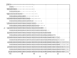
(a) $\varphi_{i}=0.85$, $b_{i}=0.2,i\in{\cal I}_{r}$.

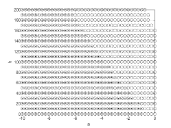
(b) $\varphi_{i}=0.85$, $b_{i}=0.1,i\in{\cal I}_{r}$.

Figure 1: Example 5: Feasible region for several values of $(a,b)\in[-10,0]\times[0,200]$. ‘$\bullet$’ indicates a feasible point using Lemma 3 with $\varphi_{i}=0.85,i\in{\cal I}_{r}$. ‘$\circ$’ indicates a feasible point using Theorem 3.

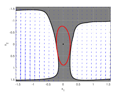
(a) The DA estimate from Lemma 3. The grey region indicates $\Omega(\varphi)$ with $(a,b)=(-8,100)$ and $\varphi_{i}=4.0789,i\in{\cal I}_{r}$. The red line indicates the boundary of the Lyapunov sublevel set ${L_{V}}(c)\subseteq\Omega(\varphi)$.

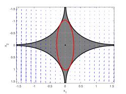
(b) The DA estimate from Theorem 3. The grey region indicates ${\cal H}(b)$ with $(a,b)=(-8,100)$ and $b_{i}=0.2603,i\in{\cal I}_{r}$. The red line indicates the boundary of the Lyapunov sublevel set ${L_{V}}(c)\subseteq{\cal H}(b)$.

Figure 2: Example 5: The DAs estimated by (a) Lemma 3 and (b) Theorem 3 with $(a,b)=(-8,100)$. The red line indicates the boundaries of the Lyapunov sublevel sets.

We note that through this single example, the conservativeness cannot be fairly compared, while it may give some insights. In the remaining parts of the paper, we provide some theoretical analysis of conservatism of different LMI conditions.

The condition in Theorem 3 necessitates solving the LMIs at all possible vertices of the hyper-rectangle described by (9). While this approach is thorough, this approach can be cumbersome to implement and computationally inefficient. A more efficient, albeit potentially more conservative, LMI condition can be achieved through the use of over-bounding techniques. These techniques obviate the need to check LMIs at every vertex of the hyper-rectangle in (9), thereby reducing the numerical and implementational complexities of Theorem 3.

Theorem 5 (Local quadratic stability II).

Suppose that the MFs are continuous. Moreover, suppose that there exist constants $b_{i}\in[0,1],i\in{\cal I}_{r}$, symmetric matrices $P=P^{T}\in{\mathbb{R}}^{n\times n}$ and $M=M^{T}\in{\mathbb{R}}^{n\times n}$ such that the following LMIs hold:

$$P\succ 0,$$

$$A_{i}^{T}P+P{A_{i}}+M\prec 0,\quad i\in{\cal I}_{r}$$ (12)

$$A_{0}^{T}P+P{A_{0}}-\sum\limits_{i=1}^{r}{{b_{i}}(A_{i}^{T}P+P{A_{i}}+M)}\prec 0$$ (13)

Then, the fuzzy system (2) is locally asymptotically stable.

Proof.

Suppose that the LMIs are feasible. Then, due to (12), one can conclude that (13) holds for $b_{i},i\in{\cal I}_{r}$ replaced with all possible combinations $\pm b_{i},i\in{\cal I}_{r}$. Therefore, the LMI in (11) hold. The remaining parts of the proof follow the same lines as in the proof of Theorem 3. This completes the proof. ∎

Example 6.

Let us consider the system in Example 5 again. The stability has been checked using Lemma 3 and Theorem 5 for several values of pairs $(a,b)\in[-10,0]\times[0,200]$. We consider $\varphi_{i}=0.85,i\in{\cal I}_{r}$ for Lemma 3 and $b_{i}=0.1,i\in{\cal I}_{r}$ for Theorem 5. Figure 3 depicts a set of feasible points for several values of pairs $(a,b)\in[-10,0]\times[0,200]$, which reveal that the region of Theorem 3 includes the region of Lemma 3.

Figure 3: Example 6: Feasible region for several values of $(a,b)\in[-10,0]\times[0,200]$. ‘$\bullet$’ indicates the feasible point of Lemma 3 with $\varphi_{i}=0.85,i\in{\cal I}_{r}$. ‘$\circ$’ indicates the feasible point of Theorem 5 with $b_{i}=0.1,i\in{\cal I}_{r}$.

III-B Local quadratic stability based on the ball bound

Until now, we have explored two versions of LMI stability conditions, both of which are based on the polytopic bound ${\cal H}(b)$ for the difference $\alpha(x)-\alpha(0)$. We will now introduce a third version that is based on a ball bound for the difference $\alpha(x)-\alpha(0)$. This alternative approach provides another avenue for stability analysis, offering a different set of trade-offs in terms of conservatism and computational complexity.

Theorem 6 (Local quadratic stability III).

Suppose that the MFs are continuous. Moreover, suppose that there exist a constant $\eta>0$, symmetric matrices $P=P^{T}\in{\mathbb{R}}^{n\times n}$, $G=G^{T}\in{\mathbb{R}}^{n\times n}$, and a matrix $M\in{\mathbb{R}}^{n\times n}$ such that the following LMIs hold:

$$P\succ 0,\quad\left[{\begin{array}[]{*{20}{c}}{\eta G+P{A_{0}}+A_{0}^{T}P}&{{\Gamma^{T}}}\\ \Gamma&{-{I_{r}}\otimes G}\end{array}}\right]\prec 0,$$ (16)

where ${\Gamma^{T}}:=\left[{\begin{array}[]{*{20}{c}}{{{(P{A_{1}}+M)}^{T}}}&\cdots&{{{(P{A_{r}}+M)}^{T}}}\end{array}}\right]$. Then, the fuzzy system (2) is locally asymptotically stable.

The proof is given in Appendix D. If the LMI condition is feasible, then any Lyapunov sublevelset ${L_{V}}(c)$ with some $c>0$ such that ${L_{V}}(c)\subseteq{\cal U}(\eta)$ is a DA, where

$${\cal U}(\eta):=\left\{{x\in{\mathbb{R}}^{n}:\sum_{i=1}^{r}{{{({\alpha_{i}}(x)-{\alpha_{i}}(0))}^{2}}}\leq\eta}\right\}.$$

Theorem 7.

Suppose that the MFs are continuous on $\cal X$. Then, there exists a ball ${\cal B}(c)$ with some $c>0$ such that ${\cal B}(c)\subseteq{\cal U}(\eta)$ for any $\eta\in[0,\infty)$.

Proof.

The proof can be completed following similar arguments as in the proof of Theorem 4. ∎

Example 7.

Let us consider the system in Example 5 again. The stability has been checked using Lemma 3 and Theorem 6 for several values of pairs $(a,b)\in[-10,0]\times[0,200]$. For Lemma 3, the derivative bounds are set to be $\varphi_{i}=0.85,i\in{\cal I}_{r}$. For Theorem 6, we consider $\eta=0.9$. Figure 4 depicts a set of feasible points for several values of pairs $(a,b)\in[-10,0]\times[0,200]$. It reveals that the region of Theorem 6 includes the region of Lemma 3.

Figure 4: Example 7: Feasible region for several values of $(a,b)\in[-10,0]\times[0,200]$. ‘$\cdot$’ indicates Lemma 3 with $\varphi_{i}=0.85,i\in{\cal I}_{r}$. ‘$\circ$’ indicates Theorem 6 with $\eta=0.9$.

Similar to Example 5, let us fix $(a,b)=(-8,100)$, and compare the largest possible DAs estimated by Lemma 3 with $\varphi_{i}=4.0789,i\in{\cal I}_{r}$ and Theorem 6 with $\eta=1.1645$. Figure 5(a) shows an estimate of a DA using Lemma 3, and Figure 5(b) depicts an estimate of a DA using Theorem 3. As can be seen from the figures, the DA estimate from Theorem 6 is larger than that from Lemma 3. Indeed, the DA estimate using Theorem 6 in Figure 5(b) is the largest one in this paper.

(a) Region of the set $\Omega(\varphi):=\{x\in{\cal X}:|{\nabla_{x}}{\alpha_{i}}{(x)^{T}}A(\alpha(x))x|\leq{\varphi_{k}},k\in{\cal I}_{r}\}$ from Lemma 3 with $(a,b)=(-10,0)$ and $\varphi_{i}=4.0789,i\in{\cal I}_{r}$. The red line indicates the boundary of the Lyapunov sublevel set ${L_{V}}(c)\subseteq\Omega(\varphi)$.

(b) Region of the set ${\cal H}(b):=\{x\in{\cal X}:|{\alpha_{i}}(x)-{\alpha_{i}}(0)|\leq{b_{i}},i\in{\cal I}_{r}\}$ from Theorem 6 with $(a,b)=(-10,0)$ and $\eta=1.1645$. The red line indicates the boundary of the Lyapunov sublevel set ${L_{V}}(c)\subseteq{\cal U}(\eta)$.

Figure 5: Example 7: The DAs estimated by (a) Lemma 3 and (b) Theorem 6 with $(a,b)=(-8,100)$. The red line indicates the boundaries of the Lyapunov sublevel sets.

Based on the findings thus far, the differences and advantages of the proposed quadratic approaches in comparison to the FLF methods can be summarized as follows: 1) The proposed quadratic methods are applicable even when the MFs are not differentiable, thereby broadening the scope of systems to which these methods can be applied; 2) The bound $|{\alpha_{i}}(x)-{\alpha_{i}}(0)|\leq{b_{i}}$ is solely dependent on the MFs, in contrast to $|{\nabla_{x}}{\alpha_{i}}{(x)^{T}}A(\alpha(x))x|\leq{\varphi_{i}},i\in{\cal I}_{r}$, which is influenced by the system dynamics $A(\alpha(x))$. Consequently, the sets ${\cal H}(b)$ and ${\cal U}(\eta)$ are independent of the system matrices $A_{i},i\in{\cal I}_{r}$, whereas $\Omega(\varphi)$ is dependent on both the system matrices and the MFs. These distinctions underscore the flexibility and applicability of the proposed quadratic approaches, particularly in scenarios where the FLF methods may be limited.

IV Analysis

In the FLF approaches, Theorem 2 reveals that conditions based on FLFs may fail to identify local stability even when the system is, in fact, locally exponentially stable. This limitation highlights an inherent conservatism in the FLF methods. Conversely, in the proposed quadratic approach, it can be proven that under certain mild assumptions, the converse statement holds true. Specifically, if the original nonlinear system is locally exponentially stable, then the LMI conditions outlined in Theorem 3, Theorem 5, and Theorem 6 are feasible. This feature enhances the applicability of the proposed quadratic stability methods.

Theorem 8 (Converse theorem I).

Suppose that the MFs are differentiable on $\cal X$, the origin is an equilibrium point of (1), and $f$ is continuously differentiable in some neighborhood of the origin. Then, the original nonlinear system (1) is locally exponentially stable around the origin if and only if the LMI condition of Theorem 3 is feasible for sufficiently small $b_{i}\in[0,1],i\in{\cal I}_{r}$.

The proof is given in Appendix E. By employing a similar line of reasoning, one can also establish the non-conservatism of the remaining two conditions, Theorem 5 and Theorem 6.

Theorem 9 (Converse theorem II).

Suppose that the MFs are differentiable on $\cal X$, the origin is an equilibrium point of (1), and $f$ is continuously differentiable in some neighborhood of the origin.

1. Then, the original nonlinear system (1) is locally exponentially stable around the origin if and only if the LMI condition of Theorem 5 is feasible for sufficiently small $b_{i}\in[0,1],i\in{\cal I}_{r}$.

2. Moreover, the original nonlinear system (1) is locally exponentially stable around the origin if and only if the LMI condition of Theorem 6 is feasible for sufficiently small $\eta>0$.

The proof is given in Appendix F. In the following, we establish less conservatism of Theorem 3 compared to Lemma 3.

Theorem 10 (Feasibility inclusion).

Suppose that the MFs are differentiable on $\cal X$, the origin is an equilibrium point of (1), and $f$ is continuously differentiable in some neighborhood of the origin. Suppose that the LMI condition of Lemma 3 is feasible for some constants $\varphi_{i}>0,i\in{\cal I}_{r}$. Then, the LMI condition of Theorem 3 is also feasible for sufficiently small $b_{i}\in[0,1],i\in{\cal I}_{r}$. However, the conserve does not hold in general.

The proof is given in Appendix G. Theorem 10 theoretically proves that Theorem 3 is less conservative than Lemma 3. Similar arguments can be applied for Theorem 5 and Theorem 6, but the results are omitted here for brevity.

Theorem 2 establishes some fundamental limitations of the FLF approaches. Despite the advantages of the proposed QLF approaches, both QLF and FLF share some fundamental limitations. Specifically, when employing either QLFs or FLFs, there exists a class of nonlinear systems whose stability cannot be identified through the associated LMI stability conditions.

Theorem 11 (Fundamental limitations).

Let us consider the nonlinear system (1), and suppose that the origin is a locally asymptotically but non-exponentially stable equilibrium point of (1). Consider the corresponding fuzzy system (2). Then, both the FLF approaches (Lemma 2 and Lemma 3) and the quadratic approaches (Theorem 3, Theorem 5, and Theorem 6) fail to identify the stability, i.e., the corresponding LMI conditions are infeasible.

The proof is given in Appendix H. In the following, we present simple examples to demonstrate the results in Theorem 11.

Example 8.

Let us consider the nonlinear system (1) with $f(x)=-x^{3}$, whose origin is asymptotically but non-exponentially stable because its solution is $x(t)=\frac{{x(0)}}{{\sqrt{1+2x{{(0)}^{2}}t}}}$. The corresponding fuzzy system is (2) with ${\alpha_{1}}(x)={x^{2}},{\alpha_{1}}(x)=1-{x^{2}},{A_{1}}=-1,{A_{2}}=0,{\cal X}=[-1,1]$. For this system, all the conditions in this paper are infeasible with any possible hyperparameters. For example, let us consider the condition of Theorem 3. In this case, $A_{0}=0$, and the LMIs in (11) are ${\delta_{1}}(A_{1}^{T}P+P{A_{1}}+M)+{\delta_{2}}(A_{2}^{T}P+P{A_{2}}+M)={\delta_{1}}(-2P+M)+{\delta_{2}}M<0$, which together with $P>0$ leads to $({\delta_{1}}+{\delta_{2}})M<2{\delta_{1}}P<0$. Since the condition should hold for all $({\delta_{1}},{\delta_{2}})\in\{-{b_{1}},{b_{1}}\}\times\{-{b_{2}},{b_{2}}\}$, when $M\geq 0$, then the condition with $({\delta_{1}},{\delta_{2}})=({b_{1}},{b_{2}})$ cannot be satisfied. In addition, when $M<0$, then the condition with $({\delta_{1}},{\delta_{2}})=({-b_{1}},{-b_{2}})$ cannot be satisfied.

We can extend the concepts in Example 8 and Theorem 11, and provide some ways to classify the set of fuzzy systems with $A_{i},i\in{\cal I}_{r}$ whose stability cannot be identified through the LMI conditions based on the FLFs. The results are given in the following theorem, which can be seen as a second version of Theorem 2.

Theorem 12 (Fundamental limitations).

Let us consider the fuzzy system (2) and suppose the system matrices $A_{i},i\in{\cal I}_{r}$ are given. If there exist some MFs $\alpha_{i}(x),i\in{\cal I}_{r}$ defined in $\cal X$ such that the nonlinear system (1) with $f(x)=\sum_{i=1}^{r}{{\alpha_{i}}(x){A_{i}}},x\in{\cal X}$ is locally asymptotically but non-exponentially stable around the origin, then for the system matrices $A_{i},i\in{\cal I}_{r}$, the FLF approaches (Lemma 2 and Lemma 3) fail to identify the stability, i.e., the corresponding LMI conditions are infeasible.

The proof is a direct corollary of Theorem 11 and is therefore omitted for brevity. The following example demonstrates Theorem 12.

Example 9.

Let us consider the linear system $\dot{x}(t)=-x(t)$, which is globally exponentially stable. The corresponding fuzzy model (2) is given with $A_{1}=-1,A_{2}=0,\alpha_{1}(x)=1,\alpha_{2}(x)=0$. For this fuzzy system, the FLF-based conditions (Lemma 2 and Lemma 3) are infeasible. This is because we can find MFs, ${\alpha_{1}}(x)={x^{2}},{\alpha_{1}}(x)=1-{x^{2}}$ in Example 8, so that $\sum_{i=1}^{r}{{\alpha_{i}}(x){A_{i}}}=f(x)=-{x^{3}},x\in{\cal X}$, and for the corresponding nonlinear system (1) with $f(x)=-x^{3}$, whose origin is asymptotically stable but non-exponentially stable.

Let us consider the nonlinear system (1) with $f(x)=\left[{\begin{array}[]{*{20}{c}}{{x_{2}}}\\ {-{x_{1}}+\mu(1+{x_{2}}){x_{2}}/2}\end{array}}\right]$ and $\mu=-2$. By the Lyapunov’s indirect method, since

$${\left.{{\nabla_{x}}f(x)}\right|_{x=0}}=\left[{\begin{array}[]{*{20}{c}}0&1\\ {-1}&{\mu/2}\end{array}}\right]=A$$

is Hurwitz, the system is locally exponentially stable at the origin. The corresponding fuzzy system (2) is defined with

$${A_{1}}=\left[{\begin{array}[]{*{20}{c}}0&1\\ {-1}&\mu\end{array}}\right],\quad{A_{2}}=\left[{\begin{array}[]{*{20}{c}}0&1\\ {-1}&0\end{array}}\right],$$ (21)

and ${\alpha_{1}}(x)=(1+{x_{2}})/2,{\alpha_{2}}(x)=1-{\alpha_{1}}(x)$, ${\cal X}=\{x\in{\mathbb{R}}^{2}:{x_{1}}\in[-1,1],{x_{2}}\in[-1,1]\}$.

Using Theorem 12, we can prove that the FLF-based conditions (Lemma 2, Lemma 3, and other conditions in the literature) are infeasible. To prove this, consider the MFs ${\alpha_{1}}(x)=1-x_{1}^{2},{\alpha_{2}}(x)=1-{\alpha_{1}}(x)$ with ${\cal X}=\{x\in{\mathbb{R}}^{2}:{x_{1}}\in[-1,1],{x_{2}}\in[-1,1]\}$. The corresponding nonlinear system (1) with $f(x)=\left[{\begin{array}[]{*{20}{c}}{{x_{2}}}\\ {\mu(1-x_{1}^{2}){x_{2}}-{x_{1}}}\end{array}}\right]$ is the well-known van der Pol oscillator, which is known to be locally asymptotically but non-exponentially stable around the origin. Therefore, by Theorem 12, the FLF-based conditions should be infeasible.

A source of conservatism of the FLF-based conditions (e.g., Lemma 2 and Lemma 3) arises from the lack of information on the MFs. These conditions are solely dependent on the system matrices $A_{i},i\in{\cal I}_{r}$, and do not incorporate any information about the structure of the MFs. In contrast, the proposed local QLF-based conditions take into account specific information about the structure of the MFs at the origin. As a result, the proposed QLF conditions can reduce the conservatism inherent in the FLF-based approaches.

Theorem 13 (Fundamental limitations).

Let us consider the fuzzy system (2), and suppose that

1. the system matrices $A_{i},i\in{\cal I}_{r}$ are given;

2. the MFs are not given, but their values at the origin $\alpha_{i}(0)=\beta_{i},i\in{\cal I}_{r}$ are given.

If there exist some MFs $\alpha_{i}(x),i\in{\cal I}_{r}$ defined in $\cal X$ such that $\alpha_{i}(0)=\beta_{i},i\in{\cal I}_{r}$ and the nonlinear system (1) with $f(x)=\sum_{i=1}^{r}{{\alpha_{i}}(x){A_{i}}},x\in{\cal X}$ is locally asymptotically but non-exponentially stable around the origin. Then, for the system matrices $A_{i},i\in{\cal I}_{r}$ and MFs’ values at the origin, the QLF approaches (Theorem 3, Theorem 5, and Theorem 3) fail to identify the stability, i.e., the corresponding LMI conditions are infeasible.

Example 10.

Here, we will cosider the two examples used in Example 9 again. Let us consider the linear system $\dot{x}(t)=-x(t)$, which is globally exponentially stable. For its fuzzy model (2) with $A_{1}=-1,A_{2}=0,\alpha_{1}(x)=1,\alpha_{2}(x)=0$, the FLF-based conditions (Lemma 2 and Lemma 3) are infeasible as shown in Example 9. In this case, $\alpha_{1}(0)=1,\alpha_{2}(0)=0$, and $A_{0}=-1$, which is Hurwitz. Therefore, with sufficiently small bounds $b_{i},i\in{\cal I}_{r}$ and $\eta$, Theorem 3, Theorem 5, and Theorem 6 are feasible.

If we consider the different MFs ${\alpha_{1}}(x)={x^{2}},{\alpha_{1}}(x)=1-{x^{2}}$ in Example 8, then ${\alpha_{1}}(0)=0,{\alpha_{1}}(x)=1$ and $A_{0}=0$. In this case, Theorem 3, Theorem 5, and Theorem 6 are feasible with any values of $b_{i},i\in{\cal I}_{r}$ and $\eta$.

Let us consider the nonlinear system (1) with $f(x)=\left[{\begin{array}[]{*{20}{c}}{{x_{2}}}\\ {-{x_{1}}+\mu(1+{x_{2}}){x_{2}}/2}\end{array}}\right]$ and $\mu=-2$, which is locally exponentially stable as shonw in Example 9. The corresponding fuzzy system (2) is defined with (21) and ${\alpha_{1}}(x)=(1+{x_{2}})/2,{\alpha_{2}}(x)=1-{\alpha_{1}}(x)$, ${\cal X}=\{x\in{\mathbb{R}}^{2}:{x_{1}}\in[-1,1],{x_{2}}\in[-1,1]\}$. Using Theorem 13, we can prove that the FLF-based conditions (Lemma 2, Lemma 3, and other conditions in the literature) are infeasible. On the other hand, we have ${\alpha_{1}}(0)=1/2,{\alpha_{2}}(0)=1/2$, and ${A_{0}}=\left[{\begin{array}[]{*{20}{c}}0&1\\ {-1}&{\mu/2}\end{array}}\right]$, which is Hurwitz. Therefore, Theorem 3, Theorem 5, and Theorem 6 are feasible with some values of $b_{i}\in[0,1],i\in{\cal I}_{r}$ and $\eta>0$.

Now, let us consider the MFs ${\alpha_{1}}(x)=1-x_{1}^{2},{\alpha_{2}}(x)=1-{\alpha_{1}}(x)$ with ${\cal X}=\{x\in{\mathbb{R}}^{2}:{x_{1}}\in[-1,1],{x_{2}}\in[-1,1]\}$. The corresponding nonlinear system (1) with $f(x)=\left[{\begin{array}[]{*{20}{c}}{{x_{2}}}\\ {\mu(1-x_{1}^{2}){x_{2}}-{x_{1}}}\end{array}}\right]$ is the well-known van der Pol oscillator, which is known to be locally asymptotically but non-exponentially stable around the origin. In this case, Theorem 3, Theorem 5, and Theorem 6 are infeasible with any values of $b_{i}\in[0,1],i\in{\cal I}_{r}$ and $\eta>0$.

Before closing this section, let us summarize the advantages of the proposed approaches: 1) As demonstrated in Theorem 8 and Theorem 9, the proposed local quadratic stability methods offer necessary and sufficient LMI conditions for ensuring local exponential stability. Furthermore, these conditions are less conservative compared to those based on FLF methods. 2) Moreover, the proposed quadratic approaches can be synergistically combined with FLF methods. The compounded effects of both methods serve to further reduce the conservatism inherent in each individual approach.

V Compounding the two effects

In the preceding section, we established that the proposed QLF approaches are less conservative than the FLF approaches. However, it is important to note that these feasibility inclusions are contingent upon the hyperparameters $\varphi_{i},i\in{\cal I}_{r}$, $b_{i},i\in{\cal I}_{r}$ and $\eta$ being variables that can be optimized. When these hyperparameters are predetermined, the feasibility inclusions no longer hold. In such instances, both the FLF and QLF methods can reduce their inherent conservatism by being compounded with each other. To elaborate, let us consider the following candidate Lyapunov function:

$$V(x)={x^{T}}{P_{0}}x+\sum_{i=1}^{r}{{\alpha_{i}}(x){x^{T}}{P_{i}}x}.$$ (22)

where $P_{0}=P_{0}^{T}\in{\mathbb{R}}^{n\times n},P_{i}=P_{i}^{T}\in{\mathbb{R}}^{n\times n},i\in{\cal I}_{r}$, which combines the FLF and QLF candidates Its time-derivative along the solution is

$$\dot{V}(x)= \sum_{i=1}^{r}{({\alpha_{i}}(x)-{\alpha_{i}}(0)){x^{T}}({P_{0}}{A_{i}}+A_{i}^{T}{P_{0}})x}$$

$$+{x^{T}}(A_{0}^{T}{P_{0}}+{P_{0}}{A_{0}})x$$

$$+\sum\limits_{j=1}^{r}{\sum\limits_{i=1}^{r}{{\alpha_{j}}(x){\alpha_{i}}(x)}}{x^{T}}({P_{j}}{A_{i}}+A_{i}^{T}{P_{j}})x$$

$$+\sum\limits_{i=1}^{r}{{{\dot{\alpha}}_{i}}(x){x^{T}}{P_{i}}x}.$$ (23)

To address the derivative ${{\dot{\alpha}}_{i}}(x)$ and the difference ${\alpha_{i}}(x)-{\alpha_{i}}(0)$, the techniques involving polytopic and ball bounds discussed in the previous section can be applied. These techniques can be variously combined to yield a range of LMI stability conditions, each with differing degrees of conservativeness. Due to space constraints, this paper will focus solely on the combination of Lemma Lemma 3 and Theorem Theorem 3. It should be noted that different combinations could lead to novel conditions, representing potential avenues for future research.

Theorem 14.

Suppose that the MFs are continuously differentiable. Moreover, suppose that there exist constants $b_{i}\in[0,1],\varphi_{i}>0,i\in{\cal I}_{r}$, symmetric matrices $P_{0}=P_{0}^{T}\in{\mathbb{R}}^{n\times n}$, $P_{i}=P_{i}^{T}\in{\mathbb{R}}^{n\times n},i\in{\cal I}_{r}$, $M=M^{T}\in{\mathbb{R}}^{n\times n}$, $N=N^{T}\in{\mathbb{R}}^{n\times n}$, and $W=W^{T}\in{\mathbb{R}}^{n\times n}$ such that the following LMIs hold:

$${P_{i}}+N\succ 0,\quad i\in{\cal I}_{r},$$ (24)

$$\sum\limits_{i=1}^{r}{{\delta_{i}}({P_{i}}+W)}+\sum\limits_{i=1}^{r}{{\alpha_{i}}(0){P_{i}}}+P_{0}\succ 0,$$ (25)

$$\sum\limits_{k=1}^{r}{{\varphi_{k}}({P_{k}}+N)}+\frac{1}{2}\left({A_{i}^{T}{P_{j}}+{P_{j}}{A_{i}}+A_{j}^{T}{P_{i}}+{P_{i}}{A_{j}}}\right)$$

$$+A_{0}^{T}P+P{A_{0}}+\sum\limits_{k=1}^{r}{{\delta_{k}}(A_{k}^{T}P+P{A_{k}}+M)}\prec 0,$$ (26)

$$\forall({\delta_{1}},{\delta_{2}},\ldots,{\delta_{r}})\in\{-{b_{1}},{b_{1}}\}\times\{-{b_{2}},{b_{2}}\}\times\cdots\times\{-{b_{r}},{b_{r}}\}$$

$$\forall(i,j)\in{\cal I}_{r}\times{\cal I}_{r},\quad i\leq j$$

Then, the fuzzy system (2) is locally asymptotically stable.

The proof is given in Appendix I. If the LMI condition of Theorem 14 is feasible, then it implies that $V(x)>0,\forall x\in{\cal H}(b)\backslash\{0\},{\nabla_{x}}V{(x)^{T}}A(\alpha)x<0,\forall x\in({\cal H}(b)\cap\Omega(\varphi))\backslash\{0\}$, and any Lyapunov sublevelset such that ${L_{V}}(c)\subseteq{\cal H}(b)\cap\Omega(\varphi)$ with some $c>0$ is a DA. In what follows, we prove that Theorem 14 is less conservative than Lemma 3 and Theorem 3.

Theorem 15 (Feasibility inclusion).

Suppose that the LMI condition of Lemma 3 is feasible for some constants $\varphi_{i}>0,i\in{\cal I}_{r}$. Then, the LMI condition of Theorem 14 is also feasible with the same constants $\varphi_{i}>0,i\in{\cal I}_{r}$ and any $b_{i}\in[0,1],i\in{\cal I}_{r}$. The conserve does not hold in general.

On the other hand, suppose that the LMI condition of Theorem 3 is feasible for some constnats $b_{i}\in[0,1],i\in{\cal I}_{r}$. Then, the LMI condition of Theorem 14 is also feasible with the same $b_{i}\in[0,1],i\in{\cal I}_{r}$ and any $\varphi_{i}>0,i\in{\cal I}_{r}$. The conserve does not hold in general.

The proof is given in Appendix J.

Example 11.

Let us consider the system in Example 5 again. The stability has been checked using Lemma 3 and Theorem 14 for several values of pairs $(a,b)\in[-10,0]\times[0,200]$. For Lemma 3, the derivative bounds are set to be $\varphi_{i}=0.85,i\in{\cal I}_{r}$. For Theorem 14, we consider $\varphi_{i}=0.85,i\in{\cal I}_{r}$ and $b_{i}=0.2,i\in{\cal I}_{r}$. Figure 6(a) depicts a set of feasible points for several values of pairs $(a,b)\in[-10,0]\times[0,200]$. It reveals that the region of Theorem 14 includes the region of Lemma 3.

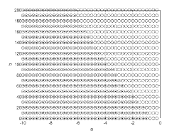
Figure 6: Example 11: Feasible region for several values of $(a,b)\in[-10,0]\times[0,200]$. ‘$\bullet$’ indicates the feasible point of Lemma 3 with $\varphi_{i}=0.85,i\in{\cal I}_{r}$. ‘$\circ$’ indicates the feasible point of Theorem 14 with $\varphi_{i}=0.85,i\in{\cal I}_{r}$ and $b_{i}=0.2,i\in{\cal I}_{r}$.

VI Conclusion and future directions

In this paper, we have introduced novel local stability conditions for T-S fuzzy systems based on QLFs. These newly formulated conditions incorporate information from the membership functions (MFs) at the origin. We have rigorously demonstrated that these conditions are both necessary and sufficient for ensuring local exponential stability. Moreover, it has been established that the proposed conditions exhibit less conservatism compared to traditional approaches based on FLFs. Additionally, we have proposed an extended Lyapunov function that combines both quadratic and FLFs, and theoretically proved that this generalization improves the aforementioned methods. To validate the theoretical claims, several illustrative examples have been provided.

The proposed methods hold promise for extension to state-feedback stabilization problems, as well as to the stability and stabilization of discrete-time T-S fuzzy systems. Various avenues exist for further reducing conservatism, including the application of additional LMI techniques to automatically estimate DAs as sublevel sets of Lyapunov functions. These topics constitute promising directions for future research.

Appendix A Proof of Theorem 1

Since the derivatives of the MFs, ${\nabla_{x}}{\alpha_{i}}(x)$, exist and continuous, and $\cal X$ is compact, ${\nabla_{x}}{\alpha_{i}}(x)$ is bounded over $\cal X$, i.e., ${\left\|{{\nabla_{x}}{\alpha_{i}}(x)}\right\|_{2}}\leq\gamma,\forall x\in{\cal X}$ for some $\gamma>0$. Therefore, we have

$$|{\nabla_{x}}{\alpha_{i}}(x)^{T}A(\alpha(x))x|\leq {\left\|{\nabla_{x}}{\alpha_{i}}(x)\right\|_{2}}{\left\|A(\alpha(x))\right\|_{2}}{\left\|x\right\|_{2}}$$

$$\leq \gamma\sum_{i=1}^{r}{\left\|A_{i}\right\|_{2}}{\left\|x\right\|_{2}},\quad\forall x\in{\cal X},$$

where the Cauchy–Schwarz inequality is used in the first inequality, and the triangle inequality is used in the second inequality. Therefore, we have $\lim_{x\to 0}|{\nabla_{x}}{\alpha_{i}}(x)A(\alpha(x))x|=0,\forall i\in{\cal I}_{r}$, and one can choose a sufficiently small ball ${\cal B}(\varepsilon)$ with some $\varepsilon>0$ such that

$$|{\nabla_{x}}{\alpha_{i}}{(x)^{T}}A(\alpha(x))x|\leq\gamma\sum\limits_{i=1}^{r}{{{\left\|{{A_{i}}}\right\|}_{2}}}\varepsilon\leq{\varphi_{i}},\quad\forall x\in{\cal B}(\varepsilon)$$

which completes the proof.

Appendix B Proof of Theorem 2

Let us consider the following simple scalar system

$$\dot{x}(t)=f(x(t))=(2\sin(x(t))-1)x(t).$$ (27)

Note that the linearization ${\left.{{\nabla_{x}}f(x)}\right|_{x=0}}=-1$ is Hurwitz. Therefore, by Lyapunov direct method, the system is locally asymptotically stable around the origin. A fuzzy system corresponding to (27) is given by (2) with ${A_{1}}=1,{A_{2}}=-1,{\alpha_{1}}(x)=\sin(x),{\alpha_{2}}(x)=(1-\sin(x)),{\cal X}=[0,\pi/2]$. Now, let us focus on the LMI condition of Lemma 3, and suppose that it is feasible, which implies that

$$P_{i}\succ 0,\quad A_{i}^{T}{P_{j}}+{P_{j}}{A_{i}}+A_{j}^{T}{P_{i}}+{P_{i}}{A_{j}}\prec 0,$$

$$\forall(i,j)\in{\cal I}_{r}\times{\cal I}_{r},\quad i\leq j.$$ (28)

are feasible. Multiplying the first and second inequality by ${\alpha_{i}}(x){\alpha_{j}}(x)$ and summing them over all ${\cal I}_{r}\times{\cal I}_{r},i\leq j$ lead to

$$P(\alpha(x))\succ 0,\quad A{(\alpha(x))^{T}}P(\alpha(x))+P(\alpha(x))A(\alpha(x))\prec 0,$$

$$x\in{\cal X},$$ (29)

which means that $A(\alpha(x))$ is Hurwitz for any $x\in{\cal X}$. As a contraposition, one concludes that if (29) does not hold, then (28) is infeasible. Moreover, if (28) is infeasible, then so is the LMI condition of Lemma 3. Returning to the fuzzy system example, one can prove that (29) does not hold at $x=\pi/2$ because ${\alpha_{1}}(\pi/2)=\sin(\pi/2)=1,{\alpha_{2}}(\pi/2)=1-\sin(\pi/2)=0$, and $A(\alpha(\pi/2))=1$. Therefore, (28) is infeasible. Therefore, the LMI condition of Lemma 3 is infeasible as well. This completes the proof.

Appendix C Proof of Theorem 3

Suppose that the LMIs in Theorem 3 are feasible. Then, it is obvious that (11) holds for all $\delta:={\left[{\begin{array}[]{*{20}{c}}{{\delta_{1}}}&{{\delta_{2}}}&\cdots&{{\delta_{r}}}\end{array}}\right]^{T}}\in H(b)$, which implies that (11) holds for all points in the intersection ${\cal H}(b)\cap\{\delta\in{\mathbb{R}}^{r}:{\bf{1}}_{r}^{T}\delta=0\}$, where ${\bf{1}}_{r}$ is the $r$-dimensional vector with all entries one. Now, setting ${\delta_{i}}={\alpha_{i}}(x)-{\alpha_{i}}(0)$, assuming $\alpha(x)-\alpha(0)\in{\cal H}(b)\cap\{\delta\in{\mathbb{R}}^{r}:{\bf{1}}_{r}^{T}\delta=0\}$, and using the null property (10), we have

$$\sum_{i=1}^{r}{({\alpha_{i}}(x)-{\alpha_{i}}(0))(A_{i}^{T}P+P{A_{i}})}+A_{0}^{T}P+P{A_{0}}\prec 0$$

for all $x\in{\cal H}(b)$. By multiplying both sides of the above inequality (7) by the state $x$ from the right and its transpose from the left and considering (6), one concludes that $\dot{V}(x(t))<0,\forall x(t)\in{\cal H}(b)\backslash\{0\}$ holds. This completes the proof.

Appendix D Proof of Theorem 6

Lemma 5.

Given matrices $U,V$ of appropriate dimensions, the following holds for any $G=G^{T}\succ 0$:

$$-U^{T}G^{-1}U-V^{T}GV\preceq U^{T}V+V^{T}U\preceq U^{T}G^{-1}U+V^{T}GV.$$

Proof.

The first inequality comes from $(G^{-1/2}U+G^{1/2}V)^{T}(G^{-1/2}U+G^{1/2}V)=U^{T}G^{-1}U+U^{T}V+V^{T}U+V^{T}GV\succeq 0$ and the reversed inequality is obtained from $(G^{-1/2}U-G^{1/2}V)^{T}(G^{-1/2}U-G^{1/2}V)=U^{T}G^{-1}U-U^{T}V-V^{T}U+V^{T}GV\succeq 0$. This completes the proof. ∎

Let us define

$${\Gamma^{T}}:=\left[{\begin{array}[]{*{20}{c}}{{{(P{A_{1}}+M)}^{T}}}&\cdots&{{{(P{A_{r}}+M)}^{T}}}\end{array}}\right],$$

and suppose that the LMIs in Theorem 6 are feasible. Applying the Schur complement leads to $\eta G+{\Gamma^{T}}{(I\otimes G)^{-1}}\Gamma+P{A_{0}}+A_{0}^{T}P\prec 0$. Then, for any $x\in{\cal U}(\eta)$, we have

$$\sum_{i=1}^{r}{(\alpha_{1}(x)-\alpha_{1}(0))^{2}}G$$

$$+\Gamma^{T}(I_{r}\otimes G)^{-1}\Gamma+PA_{0}+A_{0}^{T}P\prec 0.$$

Noting the identity $\sum_{i=1}^{r}{{({\alpha_{1}}(x)-{\alpha_{1}}(0))}^{2}}G={((\alpha(x)-\alpha(0))\otimes I_{n})^{T}}(I_{r}\otimes G)((\alpha(x)-\alpha(0))\otimes{I_{n}})$ and using Lemma 5 lead to

$$((\alpha(x)-\alpha(0))\otimes{I_{n}})^{T}\Gamma+\Gamma^{T}((\alpha(x)-\alpha(0))\otimes{I_{n}})$$

$$+A_{0}^{T}P+P{A_{0}}\prec 0,\quad x\in{\cal U}(\eta).$$

Using the null property (10) leads to (7) for all $x\in{\cal U}(\eta)$.

Appendix E Proof of Theorem 8

Lemma 6 (Lyapunov’s indirect method [1, Corollary 4.3]).

Let us consider the system (1), suppose that $f$ is continuously differentiable in some neighborhood of the origin, and the origin is an equilibrium point of (1). Then, the origin is locally exponentially stable if and only if the linearization $A={\left.{{\nabla_{x}}A(\alpha(x))x}\right|_{x=0}}$ around the origin is Hurwitz.

The sufficiency has been proved in Theorem 3. For the necessity, suppose that the original nonlinear system is locally exponentially stable around the origin. Since $A(\alpha(x))x=f(x),\forall x\in{\cal X}$, one gets

$${\nabla_{x}}f(x)= {\nabla_{x}}A(\alpha)x$$

$$= {\nabla_{x}}\left({\sum\limits_{i=1}^{r}{{\alpha_{i}}(x){A_{i}}x}}\right)$$

$$= \sum\limits_{i=1}^{r}{{A_{i}}x{\nabla_{x}}{\alpha_{i}}(x)}+\sum\limits_{i=1}^{r}{{\alpha_{i}}(x){A_{i}}}$$

Therefore, by Lyapunov’s indirect method, one concludes that

$${\left.{{\nabla_{x}}A(\alpha(x))x}\right|_{x=0}}= {\left.{\sum_{i=1}^{r}{{A_{i}}x{\nabla_{x}}{\alpha_{i}}(x)}}\right|_{x=0}}+{\left.{\sum\limits_{i=1}^{r}{{\alpha_{i}}(x){A_{i}}}}\right|_{x=0}}$$

$$= \sum\limits_{i=1}^{r}{{\alpha_{i}}(0){A_{i}}}={A_{0}}$$

is Hurwitz stable, i.e., there exists a Lyapunov matrix $P^{*}\succ 0$ such that $A_{0}^{T}P^{*}+P^{*}{A_{0}}=-Q\prec 0$ for any $Q\succ 0$. Letting $M=I$ and $P=P^{*}$ leads to

$$\sum_{i=1}^{r}{{\delta_{i}}(A_{i}^{T}P+P{A_{i}}+M)}$$

$$= \sum_{i=1}^{r}{{\delta_{i}}(A_{i}^{T}P+P{A_{i}})}+\sum\limits_{i=1}^{r}{{\delta_{i}}M}$$

$$\leq e(b)I,$$

where $e(b):=\sum_{i=1}^{r}{{{\max}_{i\in{\cal I}_{r}}}{b_{i}}\xi_{i}}$ and ${\xi_{i}}:=\max\{|{\lambda_{\max}}(A_{i}^{T}P+P{A_{i}})|,|{\lambda_{\max}}(-A_{i}^{T}P-P{A_{i}})|\}+1$. Then, one can choose sufficiently small $b_{i},i\in{\cal I}_{r}$ such that $e(b)I\prec Q$, implying $A_{0}^{T}P+P{A_{0}}+e(b)I\prec 0$ so that $A_{0}^{T}P+P{A_{0}}+\sum_{i=1}^{r}{{\delta_{i}}(A_{i}^{T}P+P{A_{i}}+M)}\prec 0$ for all $({\delta_{1}},{\delta_{2}},\ldots,{\delta_{r}})\in\{-{b_{1}},{b_{1}}\}\times\{-{b_{2}},{b_{2}}\}\times\cdots\times\{-{b_{r}},{b_{r}}\}$. This completes the proof.

Appendix F Proof of Theorem 9

The sufficiency has been proved in Theorem 5 and Theorem 6. For the necessity, suppose that the original nonlinear function is locally asymptotically stable around the origin. Then, following similar lines as in the proof of Theorem 8, there exists a Lyapunov matrix $P^{*}\succ 0$ such that $A_{0}^{T}P^{*}+P^{*}{A_{0}}=-Q\prec 0$ for any $Q\succ 0$.

Proof of the first statement: Let $M=-cI$ and choose a sufficiently large $c>0$ such that (12) is satisfied. Next, since $A_{0}^{T}P^{*}+P^{*}{A_{0}}\prec 0$ holds, letting $P=P^{*}$, one can choose a sufficiently small $b_{i}\in[0,1],i\in{\cal I}_{r}$ so that (13) holds. This completes the first part of the proof.

Proof of the second statement: Let us define

$${\Gamma^{T}}:=\left[{\begin{array}[]{*{20}{c}}{{{(P{A_{1}}+M)}^{T}}}&\cdots&{{{(P{A_{r}}+M)}^{T}}}\end{array}}\right].$$

Applying the Schur complement to (16) leads to

$$\eta G+\Gamma^{T}{(I\otimes G)^{-1}}\Gamma+P{A_{0}}+A_{0}^{T}P\prec 0.$$ (30)

Let $P=P^{*}$, $M=I$, $G=\varepsilon^{-1}I$, and $\eta\leq\varepsilon^{2}$. When $\varepsilon\to 0$, the first and second terms in (30) vanish. Therefore, one can choose a sufficiently small $\varepsilon>0$ such that the inequality in (30) holds. In other words, we can choose a sufficiently small $\eta>0$ so that the LMI condition in Theorem 6 is feasible. This completes the proof.

Appendix G Proof of Theorem 10

Suppose that the LMI condition of Lemma 2 is feasible for some constants $\varphi_{i}>0,i\in{\cal I}_{r}$. Since $P_{i}+M\succeq 0,i\in{\cal I}_{r}$, the LMIs in (5) imply that

$$A_{i}^{T}{P_{j}}+{P_{j}}{A_{i}}+A_{j}^{T}{P_{i}}+{P_{i}}{A_{j}}\prec 0,\quad\forall(i,j)\in{\cal I}\times{\cal I}_{r},i\leq j.$$

Multiplying $\alpha_{i}(x)\alpha_{j}(x)$ on both sides of the above inequalities and summing them over all $i,j\in{\cal I}_{r},i\leq j$ lead to

$$A{(\alpha(x))^{T}}P(\alpha(x))+P(\alpha(x))A(\alpha(x))\prec 0,\forall x\in{\cal X}$$

with $P(\alpha(x))=\sum_{i=1}^{r}{{\alpha_{i}}(x){P_{i}}}$. Letting $x=0$ yields $A{(\alpha(0))^{T}}P(\alpha(0))+P(\alpha(0))A(\alpha(0))\prec 0\Rightarrow A_{0}^{T}P+P{A_{0}}\prec 0$ with $P=P(\alpha(0))$, which means that $A_{0}$ is Hurwitz. Now, it is clear that one can choose sufficiently small $b_{i}>0,i\in{\cal I}_{r}$ so that (11) holds.

To prove the converse, let us consider the fuzzy system (2) with ${A_{1}}=1,{A_{2}}=-1,{\alpha_{1}}(x)=\sin(x),{\alpha_{2}}(x)=(1-\sin(x)),{\cal X}=[0,\pi/2]$. Noting ${\alpha_{1}}(0)=0,{\alpha_{2}}(0)=1$, we have ${A_{0}}={\alpha_{1}}(0){A_{1}}+{\alpha_{2}}(0){A_{2}}=-1$, which is Hurwitz. Therefore, following the same steps as in the proof of Theorem 8, one concludes that the LMI condition of Theorem 3 is also feasible for sufficiently small $b_{i},i\in{\cal I}_{r}$. For this system, we can prove that the LMI condition of Lemma 2 is not feasible for any constants $\varphi_{i}>0,i\in{\cal I}_{r}$. In particular, ${\varphi_{1}}{P_{1}}+{\varphi_{2}}{P_{2}}+A_{1}^{T}{P_{1}}+{P_{1}}{A_{1}}+A_{1}^{T}{P_{1}}+{P_{1}}{A_{1}}\prec 0$ implies ${P_{1}}<-\frac{{{\varphi_{2}}}}{{1+{\varphi_{1}}}}{P_{2}}$, which cannot be satisfies with $P_{1}>0,P_{2}>0$. This completes the proof.

Appendix H Proof of Theorem 11

Let us consider a nonlinear system (1) which is locally asymptotically but non-exponentially stable. By contradiction, suppose that the FLF approaches (Lemma 2 and Lemma 3) and the QLF approaches (Theorem 3, Theorem 5, and Theorem 6) found a feasible solution. This implies that there exists some Lyapunov sublevel set ${L_{V}}(c)$ with some $c>0$ such that it is a DA. To proceed further, let us consider the fuzzy Lypaunov function $V(x)={x^{T}}P(\alpha(x))x$. Then, for any $x(t)\in{L_{V}}(c)$, we have $\frac{d}{{dt}}V(x(t))\leq-\varepsilon x{(t)^{T}}x(t)<0$ for all $x(t)\neq 0$ and for a sufficiently small constant $\varepsilon>0$. Noting ${\min_{i\in{\cal I}_{r}}}{\lambda_{\min}}({P_{i}}){x^{T}}x\leq{x^{T}}P(\alpha(x))x\leq{\max_{i\in{\cal I}_{r}}}{\lambda_{\max}}({P_{i}}){x^{T}}x$, this implies that

$$\frac{d}{{dt}}V(x(t))\leq-\left({\frac{\varepsilon}{{{{\max}_{i\in{\cal I}_{r}}}{\lambda_{\max}}({P_{i}})}}}\right)V(x(t)),\forall x(t)\neq 0$$

and equivalently, $V(x(t))\leq\exp\left({-\frac{{\varepsilon t}}{{{{\max}_{i\in{\cal I}_{r}}}{\lambda_{\max}}({P_{i}})}}}\right)V(0)$. Then, it follows that ${\left\|{x(t)}\right\|_{2}}\leq\sqrt{\frac{1}{{{{\min}_{i\in{\cal I}_{r}}}{\lambda_{\min}}({P_{i}})}}\exp\left({-\frac{{\varepsilon t}}{{{{\max}_{i\in{\cal I}_{r}}}{\lambda_{\max}}({P_{i}})}}}\right)V(0)}$. Therefore, (1) is locally exponentially stable, and it contradicts with the hypothesis that (1) is locally asymptotically but non-exponentially stable. This completes the proof.

Appendix I Proof of Theorem 14

The proof is a combination of the proof of Lemma 3 and Theorem 3. Suppose that the LMIs in Theorem 14 are feasible. Then, one can let ${\varphi_{i}}={{\dot{\alpha}}_{i}}(x(t)),i\in{\cal I}_{r}$ and ${\delta_{i}}={\alpha_{i}}(x(t))-{\alpha_{i}}(0),i\in{\cal I}_{r}$ in (26). Using the null effects $\sum_{k=1}^{r}{{{\dot{\alpha}}_{k}}(x(t))}=0$, $\sum_{i=1}^{r}{({\alpha_{i}}(x(t))-{\alpha_{i}}(0))}=0$, using the bound (24), multiplying the inequality (26) by $\alpha_{i}(x(t))\alpha_{j}(x(t))$, and summing it over all $(i,i)\in{\cal I}_{r}\times{\cal I}_{r},i\leq j$ lead to

$$\sum_{i=1}^{r}{({\alpha_{i}}(x(t))-{\alpha_{i}}(0))({P_{0}}{A_{i}}+A_{i}^{T}{P_{0}})}+A_{0}^{T}{P_{0}}+{P_{0}}{A_{0}}$$

$$+\sum_{j=1}^{r}{\sum_{i=1}^{r}{{\alpha_{j}}(x(t)){\alpha_{i}}(x(t))}}({P_{j}}{A_{i}}+A_{i}^{T}{P_{j}})$$

$$+\sum_{i=1}^{r}{{{\dot{\alpha}}_{i}}(x(t)){P_{i}}}\prec 0,\quad\forall x\in{\cal H}(b)\cap\Omega(\varphi)$$

which holds if and only if the time-derivative of the Lyapunov function along the solution (23) is negative definite.

On the other hand, letting ${\delta_{i}}={\alpha_{i}}(x(t))-{\alpha_{i}}(0),i\in{\cal I}_{r}$ in (25) and using the null effect $\sum_{i=1}^{r}{({\alpha_{i}}(x(t))-{\alpha_{i}}(0))}=0$, one has ${P_{0}}+\sum_{i=1}^{r}{{\alpha_{i}}(x){P_{i}}}\succ 0,\forall x\in{\cal H}(b)\Leftrightarrow V(x)>0,\forall x\in{\cal H}(b)\backslash\{0\}$. This completes the proof.

Appendix J Proof of Theorem 15

Suppose that the LMI condition of Lemma 3 is feasible for some constants $\varphi_{i}>0,i\in{\cal I}_{r}$. Then, for any $b_{i}\in[0,1],i\in{\cal I}_{r}$, it can be easily proved that with $P_{0}=\varepsilon_{1}I$, $M=\varepsilon_{2}I$, and sufficiently small $\varepsilon_{1},\varepsilon_{2}>0$, (26) holds. Moreover, it is clear that (24) and (25) hold.

On the other hand, suppose that the LMI condition of Theorem 3 is feasible for some constnats $b_{i}\in[0,1],i\in{\cal I}_{r}$. Then, for any $\varphi_{i}\in[0,1],i\in{\cal I}_{r}$, it can be easily proved that with $P_{i}=\varepsilon_{i}I,i\in{\cal I}_{r}$, $N=\varepsilon_{r+1}I$ and sufficiently small $\varepsilon_{i}>0,i\in{\cal I}_{r}$, $\varepsilon_{r+1}>0$, (26) holds. Moreover, it is clear that (24) and (25) hold. This completes the proof.

References

• [1] H. K. Khalil, Nonlinear systems, 2002.
• [2] K. Tanaka and H. O. Wang, Fuzzy control systems design and analysis: a linear matrix inequality approach.   John Wiley & Sons, 2004.
• [3] S. Boyd, L. El Ghaoui, E. Feron, and V. Balakrishnan, Linear matrix inequalities in system and control theory.   SIAM, 1994.
• [4] A.-T. Nguyen, T. Taniguchi, L. Eciolaza, V. Campos, R. Palhares, and M. Sugeno, “Fuzzy control systems: Past, present and future,” IEEE Computational Intelligence Magazine, vol. 14, no. 1, pp. 56–68, 2019.
• [5] C.-H. Fang, Y.-S. Liu, S.-W. Kau, L. Hong, and C.-H. Lee, “A new lmi-based approach to relaxed quadratic stabilization of ts fuzzy control systems,” IEEE Transactions on fuzzy systems, vol. 14, no. 3, pp. 386–397, 2006.
• [6] E. Kim and H. Lee, “New approaches to relaxed quadratic stability condition of fuzzy control systems,” IEEE Transactions on Fuzzy systems, vol. 8, no. 5, pp. 523–534, 2000.
• [7] A. Sala and C. Ariño, “Asymptotically necessary and sufficient conditions for stability and performance in fuzzy control: Applications of polya’s theorem,” Fuzzy sets and systems, vol. 158, no. 24, pp. 2671–2686, 2007.
• [8] R. C. Oliveira and P. L. Peres, “Parameter-dependent lmis in robust analysis: Characterization of homogeneous polynomially parameter-dependent solutions via lmi relaxations,” IEEE Transactions on Automatic Control, vol. 52, no. 7, pp. 1334–1340, 2007.
• [9] A. Sala and C. Arino, “Relaxed stability and performance conditions for takagi–sugeno fuzzy systems with knowledge on membership function overlap,” IEEE Transactions on Systems, Man, and Cybernetics, Part B (Cybernetics), vol. 37, no. 3, pp. 727–732, 2007.
• [10] M. Narimani and H.-K. Lam, “Relaxed lmi-based stability conditions for takagi–sugeno fuzzy control systems using regional-membership-function-shape-dependent analysis approach,” IEEE Transactions on Fuzzy Systems, vol. 17, no. 5, pp. 1221–1228, 2009.
• [11] A. Kruszewski, A. Sala, T. M. Guerra, and C. Arino, “A triangulation approach to asymptotically exact conditions for fuzzy summations,” IEEE Transactions on Fuzzy Systems, vol. 17, no. 5, pp. 985–994, 2009.
• [12] M. Johansson, A. Rantzer, and K.-E. Arzen, “Piecewise quadratic stability of fuzzy systems,” IEEE Transactions on Fuzzy Systems, vol. 7, no. 6, pp. 713–722, 1999.
• [13] G. Feng, “Controller synthesis of fuzzy dynamic systems based on piecewise lyapunov functions,” IEEE Transactions on Fuzzy Systems, vol. 11, no. 5, pp. 605–612, 2003.
• [14] V. C. Campos, F. O. Souza, L. A. Tôrres, and R. M. Palhares, “New stability conditions based on piecewise fuzzy lyapunov functions and tensor product transformations,” IEEE Transactions on Fuzzy Systems, vol. 21, no. 4, pp. 748–760, 2012.
• [15] K. Tanaka, T. Hori, and H. O. Wang, “A multiple lyapunov function approach to stabilization of fuzzy control systems,” IEEE Transactions on fuzzy systems, vol. 11, no. 4, pp. 582–589, 2003.
• [16] L. A. Mozelli, R. M. Palhares, F. Souza, and E. M. Mendes, “Reducing conservativeness in recent stability conditions of ts fuzzy systems,” Automatica, vol. 45, no. 6, pp. 1580–1583, 2009.
• [17] T. M. Guerra and L. Vermeiren, “Lmi-based relaxed nonquadratic stabilization conditions for nonlinear systems in the takagi–sugeno’s form,” Automatica, vol. 40, no. 5, pp. 823–829, 2004.
• [18] B. Ding, H. Sun, and P. Yang, “Further studies on lmi-based relaxed stabilization conditions for nonlinear systems in takagi–sugeno’s form,” Automatica, vol. 42, no. 3, pp. 503–508, 2006.
• [19] D. H. Lee, J. B. Park, and Y. H. Joo, “Improvement on nonquadratic stabilization of discrete-time takagi–sugeno fuzzy systems: Multiple-parameterization approach,” IEEE Transactions on Fuzzy Systems, vol. 18, no. 2, pp. 425–429, 2010.
• [20] ——, “A new fuzzy lyapunov function for relaxed stability condition of continuous-time takagi–sugeno fuzzy systems,” IEEE Transactions on Fuzzy Systems, vol. 19, no. 4, pp. 785–791, 2011.
• [21] D. H. Lee and Y. H. Joo, “On the generalized local stability and local stabilization conditions for discrete-time takagi–sugeno fuzzy systems,” IEEE Transactions on Fuzzy Systems, vol. 22, no. 6, pp. 1654–1668, 2014.
• [22] D. H. Lee et al., “Relaxed lmi conditions for local stability and local stabilization of continuous-time takagi–sugeno fuzzy systems,” IEEE Transactions on Cybernetics, vol. 44, no. 3, pp. 394–405, 2013.
• [23] B. Ding, “Homogeneous polynomially nonquadratic stabilization of discrete-time takagi–sugeno systems via nonparallel distributed compensation law,” IEEE Transactions on Fuzzy Systems, vol. 18, no. 5, pp. 994–1000, 2010.
• [24] B.-J. Rhee and S. Won, “A new fuzzy lyapunov function approach for a takagi–sugeno fuzzy control system design,” Fuzzy sets and systems, vol. 157, no. 9, pp. 1211–1228, 2006.
• [25] K. Tanaka, H. Yoshida, H. Ohtake, and H. O. Wang, “A sum-of-squares approach to modeling and control of nonlinear dynamical systems with polynomial fuzzy systems,” IEEE Transactions on Fuzzy systems, vol. 17, no. 4, pp. 911–922, 2008.
• [26] A. Sala and C. Arino, “Polynomial fuzzy models for nonlinear control: A taylor series approach,” IEEE Transactions on Fuzzy Systems, vol. 17, no. 6, pp. 1284–1295, 2009.
• [27] H.-K. Lam, “Polynomial fuzzy-model-based control systems: Stability analysis via piecewise-linear membership functions,” IEEE Transactions on Fuzzy Systems, vol. 19, no. 3, pp. 588–593, 2011.
• [28] M. Bernal, A. Sala, A. Jaadari, and T.-M. Guerra, “Stability analysis of polynomial fuzzy models via polynomial fuzzy lyapunov functions,” Fuzzy Sets and Systems, vol. 185, no. 1, pp. 5–14, 2011.
• [29] A. Kruszewski, R. Wang, and T.-M. Guerra, “Nonquadratic stabilization conditions for a class of uncertain nonlinear discrete time ts fuzzy models: A new approach,” IEEE Transactions on Automatic Control, vol. 53, no. 2, pp. 606–611, 2008.
• [30] D. H. Lee, J. B. Park, and Y. H. Joo, “Approaches to extended non-quadratic stability and stabilization conditions for discrete-time takagi–sugeno fuzzy systems,” Automatica, vol. 47, no. 3, pp. 534–538, 2011.
• [31] M. Bernal and T. M. Guerra, “Generalized nonquadratic stability of continuous-time takagi–sugeno models,” IEEE Transactions on Fuzzy Systems, vol. 18, no. 4, pp. 815–822, 2010.
• [32] J.-T. Pan, T. M. Guerra, S.-M. Fei, and A. Jaadari, “Nonquadratic stabilization of continuous t–s fuzzy models: Lmi solution for a local approach,” IEEE Transactions on Fuzzy Systems, vol. 20, no. 3, pp. 594–602, 2011.
• [33] D. H. Lee, J. B. Park, and Y. H. Joo, “A fuzzy lyapunov function approach to estimating the domain of attraction for continuous-time takagi–sugeno fuzzy systems,” Information Sciences, vol. 185, no. 1, pp. 230–248, 2012.
• [34] K. Tanaka and T. Kosaki, “Design of a stable fuzzy controller for an articulated vehicle,” IEEE Transactions on Systems, Man, and Cybernetics, Part B (Cybernetics), vol. 27, no. 3, pp. 552–558, 1997.