Advantages of the Kirkwood-Dirac distribution among general quasi-probabilities for finite-state quantum systems

Abstract

We investigate features of the quasi-joint-probability distribution for finite-state quantum systems, especially the two-state and three-state quantum systems, comparing different types of quasi-joint-probability distributions based on the general framework of quasi-classicalization. We show from two perspectives that the Kirkwood-Dirac distribution is the quasi-joint-probability distribution that behaves nicely for the finite-state quantum systems. One is the similarity to the genuine probability and the other is the information that we can obtain from the quasi-probability. By introducing the concept of the possible values of observables, we show for the finite-state quantum systems that the Kirkwood-Dirac distribution behaves more similarly to the genuine probability distribution in contrast to most of the other quasi-probabilities including the Wigner function. We also prove that the states of the two-state and three-state quantum systems can be completely distinguished by the Kirkwood-Dirac distribution of only two directions of the spin and point out for the two-state system that the imaginary part of the quasi-probability is essential for the distinguishability of the state.

xxxx, xxx

1 Introduction

Because of the non-commutativity of observables, it is well-known that the genuine joint-probability distribution of multiple observables cannot be defined in quantum theory. However, in order to obtain an intuitive interpretation of the quantum theory, many attempts have been made to build a quantum analogue of the joint-probability distribution, which is called the quasi-joint-probability distribution, or shortly, quasi-probability by many pioneers including Wigner and Kirkwood Wigner1932; Kirkwood1933; Dirac1945; Margenau1961; Born1925; Husimi1940; Glauber1963; Sudarshan1963. Though the quasi-probabilities had been at first defined in a heuristic manner, attempts to construct the general treatment of the quasi-probabilities were also made. The unification of some of the quasi-probabilities of the position and momentum was proposed by Cohen Cohen2005, and later all the quasi-probabilities mentioned above were indeed unified in the general framework of quasi-classicalization by Lee and Tsutsui Lee2017; Lee2018.

Perhaps the most famous one of these quasi-probabilities is the Wigner function Wigner1932, which is an example of the quasi-joint-probability distribution of the position and the momentum of a particle. The Wigner function is useful in the sense that its negativity shows the non-classicality Kenfack2004, especially the contextuality Spekkens2008; Booth2022; haferkamp2021 of the state. It is indeed widely used in the field of quantum optics and quantum computation Delfosse2015; Raussendorf2017; Maffei2023.

On the other hand, there is not much research that focused on the quasi-probability for other systems, such as the two-state quantum system. Finite-state systems has appeared only as a mere example Margenau1961 and has not explored seriously. Indeed, it became possible to compare different types of quasi-probabilities systematically only after the unification by Lee and Tsutsui Lee2017; Lee2018. The question here is which quasi-probabilities behave more nicely, which behave more similarly to genuine probability and which give us more information about the state. This type of argument was conducted by Hofmann Hofmann2014, who pointed out that some reasonable condition for the quasi-probability to behave more similarly to the genuine probability requires it to be the Kirkwood-Dirac distribution Hofmann2014. The Kirkwood-Dirac distribution Kirkwood1933; Dirac1945 is also useful in that it gives a statistical interpretation Ozawa2011; Morita2013; Lee2017; Lee2018 of the weak value introduced by Aharonov Aharonov1964; Aharonov1988, though it is not much better known than the Wigner function.

In the present work, we investigate features of the quasi-joint-probability distribution for finite-state quantum systems, especially the two-state and three-state quantum systems and compare among types of quasi-probabilities. Through the following argument, we will show from a point of view different from Hofmann’s work that the Kirkwood-Dirac distribution is the quasi-joint-probability distribution that behaves nicely in finite-state systems contrary to optical systems.

In Sec. 2, we first review the general framework of the quasi-joint-probability distribution and point out a problem that uniquely occurs for finite-state systems. We then show the superiority of the Kirkwood-Dirac distribution in the two-state quantum system in Sec. 3 and the three-state quantum system in Sec. LABEL:Quasi-Probabilities_for_Three-State_Quantum_System. In Sec. LABEL:Quasi-Probabilities_for_General_Finite-State_Quantum_System, we refer to a general statement for the finite-state quantum systems.

2 Quasi-Joint-Probability Distributions

The purpose of the present section is to introduce the concept of the quasi-joint-probability distribution and to review its general framework Lee2017; Lee2018. We first look at the Born rule and functional calculus, which is the trivial case of quasi-classicalization and the quantization in the sense that they can be uniquely defined in the standard quantum theory. We then define the quasi-joint-probability distribution and the quantization of general physical quantities as an extension of the trivial case by introducing the quasi-joint-spectrum distributionLee2018. Through this framework, the duality of quantization and quasi-classicalization together with the arbitrariness of their definition are revealed. We then look at the real quasi-classicalization, a quasi-classicalization that generates a real-valued quasi-joint-probability distribution with respect to arbitrary states Lee2018. At the end of this section, we will point out an interesting feature of the quasi-joint-probability distribution of finite-state quantum systems.

2.1 The general framework of quasi-probabilities and quantizations

In quantum theory, an orthogonal projection $\hat{E}_{A}(a)$ onto the eigenspace corresponding to the eigenvalue $a$ of an observable $A$ plays an important role. By using the orthogonal projection, the probability distribution of the value $a$ of the observable $A$ with respect to the state described by a density operator $\rho$ is derived from the Born rule as in

$$P_{\rho}(a)=\mathrm{Tr}[E_{A}(a)\,\rho\,].$$ (1)

The quantization of an observable described as an univariable function of $A$ is also derived by using the orthogonal projection from the functional calculus:

$$f(A)=\int_{-\infty}^{\infty}f(a)E_{A}(a)\mathrm{d}a.$$ (2)

Here, $A$ denotes the operator which is the expressions of an physical quantity in quantum theory and $a$ denotes the value which is the expression of the physical quantity in classical theory.

Since the mutual orthogonal projection for the combination of non-commutative observables cannot be defined, we cannot naively extend the method above in order to find a joint-probability distribution of multiple observables or to quantize a physical quantity described as a multivariable function of observables. In fact, there do not exist any joint-probability distributions of non-commutative observables that satisfy the axioms of the probability:

$$(\mathrm{i})\;\;\;^{\forall}E\in\mathfrak{B},\;P(E)\in\mathbb{R}_{\geq 0},\;\;\;\mbox{where}\;\mathfrak{B}\;\mbox{is a}\;\sigma\mbox{-algebre of the sample space}\;\Omega;$$

$$(\mathrm{ii})\;\;\;P(\Omega)=1;$$ (3)

$$(\mathrm{iii})\;\;\;P\Bigl{(}\bigcup_{i=1}^{\infty}E_{i}\Bigr{)}=\sum_{i=1}^{\infty}P(E_{i})\;\;\;\mathrm{for\;disjoint\;sets}\;\{E_{i}\in\mathfrak{B}\}.$$

However, it is known that we can define a “quasi-joint-probability distribution”, which satisfies only (ii) and (iii) of the axioms of the probability by extending the method above.

As a special case of functional calculus (2), the quantization of $e^{-isA}$ is given by

$$e^{-isA}=\int_{-\infty}^{\infty}e^{-isa}E_{A}(a)da.$$ (4)

This formula is also understood as the Fourier transform $\mathcal{F}$ of the projection operator:

$$e^{-isA}=\sqrt{2\pi}\mathcal{F}\bigl{(}E_{A}(a)\bigr{)}(s).$$ (5)

Therefore, we can conversely consider the orthogonal projection as the inverse Fourier transform of $e^{-is\hat{A}}$:

$$E_{A}(a)=\frac{1}{\sqrt{2\pi}}\mathcal{F}^{-1}\bigl{(}e^{-isA}\bigl{)}(a).$$ (6)

As an extension of this formalism, we define the $hashed\;operator$ Lee2018:

$$\hat{\#}_{\bm{A}}(\bm{s})\coloneqq\{$$ a suitable ‘mixture’ of the ‘disintegrated’ components of

$$\mbox{the unitary groups}\;e^{-is\hat{A}_{1}},...,e^{-is\hat{A}_{n}}\},\;\;\bm{s}\in\mathbb{R}^{n},\;\bm{A}=(A_{1},...,A_{n})$$ (7)

and the quasi-joint-spectral distribution (QJSD) as the inverse Fourier transform of the hashed operator Lee2018:

$$\#_{\bm{A}}(\bm{a})\coloneqq\frac{1}{\sqrt{2\pi}^{n}}\mathcal{F}^{-1}\Bigl{(}\hat{\#}_{\bm{A}}(\bm{s})\Bigr{)}(\bm{a}).$$ (8)

Note that $\bm{A}$, thus also $\hat{\bm{A}}$ and $\bm{a}$, are now multivariable vectors.

The important point here is that the definition of the hashed operator, and thus that of quasi-joint-spectrum distribution, has arbitrariness. In the case $\bm{A}=(A,\;B)$, candidates of the hashed operator include

$$\hat{\#}^{\mathrm{K}}_{(A,B)}(s,t)=e^{-isA}e^{-itB},$$ (9)

$$\hat{\#}^{\mathrm{S_{\alpha}}}_{(A,B)}(s,t)=e^{-i\alpha sA}e^{-itB}e^{-i(1-\alpha)sA},$$ (10)

$$\hat{\#}^{\mathrm{M_{\alpha}}}_{(A,B)}(s,t)=\frac{1+\alpha}{2}e^{-isA}e^{-it\hat{B}}+\frac{1-\alpha}{2}e^{-itB}e^{-isA},$$ (11)

$$\hat{\#}^{\mathrm{W}}_{(A,B)}(s,t)=e^{-i(sA+tB)}=\lim_{N\to\infty}(e^{-i\frac{s}{N}A}e^{-i\frac{t}{N}B})^{N},$$ (12)

$$\hat{\#}^{\mathrm{B}}_{(A,B)}(s,t)=\frac{1}{2}\int_{-1}^{1}e^{-i\frac{1-k}{2}sA}e^{-itB}e^{-i\frac{1+k}{2}sA}\,\mathrm{d}k,$$ (13)

where K, W, M and B in the superscripts refer to the Kirkwood-Dirac, Wigner, Margenau-Hill and Born-Jordan respectively, while S does not stand for a specific name. By using quasi-joint-spectrum distributions, the quasi-joint-probability distribution is defined analogously to the Born rule Lee2018:

$$P_{\rho}(\bm{a})=\mathrm{Tr}[\#_{\bm{A}}(\bm{a})\,\rho\,].$$ (14)

In particular, the quasi-joint-probability distribution with respect to a pure state is calculated as

$$P_{\psi}(\bm{a})=\bra{\psi}\#_{\bm{A}}(\bm{a})\ket{\psi}.$$ (15)

Quantizations of a physical quantity $f(\bm{A})$, which is expressed as a multivariable function of $\bm{A}$, is also derived from QJSD Lee2018 as in

$$f(\bm{A})=\int_{\mathbb{R}^{n}}f(\bm{a})\;\#_{\bm{A}}(\bm{a})\;\mathrm{d}^{n}\bm{a}.$$ (16)

Since the quasi-joint-probability distribution and the quantization of a physical quantity are defined by using QJSDs, they also have arbitrariness in its definition. The quasi-joint-probability distribution generated from the hashed operator of the specific form

$$\hat{\#}_{\bm{A}}^{\mathrm{K}}(\bm{s})\coloneqq\prod_{k=1}^{n}e^{-is_{k}A_{k}}$$ (17)

is known as the Kirkwood-Dirac distribution Lee2018; Kirkwood1933; Dirac1945:

$$K_{\rho}(\bm{a})\coloneqq\mathrm{Tr}[\#^{\mathrm{K}}_{\bm{A}}(\bm{a})\,\rho\,].$$ (18)

The quasi-joint-probability distribution generated from the hashed operator of the form

$$\hat{\#}_{\bm{A}}^{\mathrm{W}}(\bm{s})\coloneqq e^{-i\sum_{k=1}^{n}s_{k}A_{k}}$$ (19)

is a generalization of the Wigner function Lee2018; Wigner1932; Weyl1927:

$$W_{\rho}(\bm{a})\coloneqq\mathrm{Tr}[\#^{\mathrm{W}}_{\bm{A}}(\bm{a})\,\rho\,].$$ (20)

Other quasi-joint-probability distributions are also understood as special cases of this formalism.

Although they have arbitrariness in their definition, there are conditions that quasi-joint-probability distributions must satisfy except for (ii) and (iii) of the axioms of the probability. The marginal probability distribution of $A_{k}$ calculated as

$$P^{A_{k}}_{\rho}(a_{k})\coloneqq\int_{\mathbb{R}^{n-1}}P^{\bm{A}}_{\rho}(\bm{a})\;\mathrm{d}a_{1}...\mathrm{d}a_{k-1}\mathrm{d}a_{k+1}...\mathrm{d}a_{n}\;\;\;(k=1,2,...,n)$$ (21)

should express the probability that the observable $A_{k}$ takes $a_{k}$ in the state $\rho$, but it is something that can be computed from the standard quantum theory with no arbitrariness:

$$P^{A_{k}}_{\rho}(a_{k})=\mathrm{Tr}[E_{A_{k}}(a_{k})\,\rho\,].$$ (22)

Therefore the marginal probability distributions (21) must be consistent with Eq. (22). Thanks to the definitions (2.1), (8) and (14), any quasi-joint-probability distributions naturally fulfill this condition. Note that distributions which do not satisfy this condition, such as the Husimi function Husimi1940, are not included in this definition of quasi-joint-probability distribution, though it can also be understood as an extension of this formalismLee2018.

The duality of quantization and “quasi-classicalization”, which is the map from a density operator to a quasi-joint-probability distribution, is easily understood from the equivalence between two ways of computing the quasi-expectation-value of a physical quantity $f(\bm{A})$ in the state $\rho$; see the diagram in Fig. 1. One way is to quasi-classicalize the state (that is, to map the state $\hat{\rho}$ to the quasi-joint-probability distribution $P_{\rho}(\bm{a})$) and to compute the expectation value in classical theory as in

$$\langle f(\bm{A})\rangle=\int_{\mathbb{R}^{n}}f(\bm{a})P_{\rho}(\bm{a})\mathrm{d}^{n}\bm{a}.$$ (23)

The other way is to quantize the physical quantity and to compute the expectation value in quantum theory as in

$$\langle f(\bm{A})\rangle=\mathrm{Tr}[f(\bm{A})\,\rho\,].$$ (24)

The fact that both Eqs. (23) and (24) give the same quasi-expectation value implies the duality of quasi-classicalization and quantization.

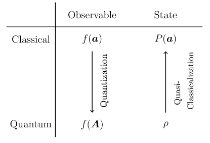
Figure 1: The duality of quasi-classicalization and quantization.

2.2 Quasi-classicalizations generating real quasi-probabilities

Though a quasi-joint-probability distribution generally takes complex values contrary to the regular probability distributions, some quasi-joint-probability distributions stay real. In this subsection, we will look at which quasi-classicalization generates a quasi-joint-probability distributions that takes only real values.

Since the density operator is generally Hermitian, the statement that a quasi-joint-probability distribution takes real values with respect to arbitrary states, which we refer to as a real quasi-classicalization, is equivalent to the statement that the corresponding QJSD is Hermitian

$$^{\forall}\rho,\;P^{\mathrm{T}}_{\rho}(\bm{a})\in\mathbb{R}\iff\#^{\mathrm{T}}_{\bm{A}}(\bm{a})=\#^{\mathrm{T}\dagger}_{\bm{A}}(\bm{a}),$$ (25)

where $\mathrm{T}=\mathrm{K,\,W}$ and so on. Since the Hermitian conjugate of a QJSD is expressed as

$$\#^{\mathrm{T}\dagger}_{\bm{A}}(\bm{a}) =\frac{1}{\sqrt{2\pi}^{n}}\Bigl{(}\mathcal{F}^{-1}\bigl{(}\hat{\#}^{\mathrm{T}}_{\bm{A}}(\bm{s})\bigr{)}(\bm{a})\Bigr{)}^{\dagger}$$

$$=\frac{1}{(2\pi)^{n}}\int_{\mathbb{R}^{n}}\hat{\#}^{\mathrm{T}\dagger}_{\bm{A}}(\bm{s})e^{-i\bm{s}\cdot\bm{a}}\;\mathrm{d}^{n}\bm{s}$$

$$=\frac{1}{(2\pi)^{n}}\int_{\mathbb{R}^{n}}\hat{\#}^{\mathrm{T}\dagger}_{\bm{A}}(-\bm{s})e^{i\bm{s}\cdot\bm{a}}\;\mathrm{d}^{n}\bm{s}$$

$$=\frac{1}{\sqrt{2\pi}^{n}}\mathcal{F}^{-1}\bigl{(}\hat{\#}^{\mathrm{T}\dagger}_{\bm{A}}(-\bm{s})\bigr{)}(\bm{a}),$$ (26)

the reality of a quasi-classicalization can be also expressed as the following relation of hashed operators Lee2018:

$$^{\forall}\rho,\;P^{\mathrm{T}}_{\rho}(\bm{a})\in\mathbb{R}\iff\#^{\mathrm{T}}_{\bm{A}}(\bm{a})=\#^{\mathrm{T}\dagger}_{\bm{A}}(\bm{a})\iff\hat{\#}^{\mathrm{T}}_{\bm{A}}(\bm{s})=\hat{\#}^{\mathrm{T}\dagger}_{\bm{A}}(-\bm{s}).$$ (27)

Therefore, we can see that the Wigner distribution (20) always takes real values because Eq. (19) satisfies the right-most condition of Eq. (27), but the Kirkwood-Dirac distribution (18) can take complex values because Eq. (17) does not satisfy it.

Real quantization, a quantization corresponding to a real quasi-classicalization, is also meaningful. A real quantization quantizes every physical quantity to a Hermitian operators Lee2018 because

$$\Bigl{(}f^{\mathrm{T}}(\bm{A})\Bigr{)}^{\dagger} =\int_{\mathbb{R}^{n}}f(\bm{a})\;\#^{\mathrm{T}\dagger}_{\bm{A}}(\bm{a})\;\mathrm{d}^{n}\bm{a}.$$ (28)

$$=f^{\mathrm{T}}(\hat{\bm{A}})$$ (29)

if $\#^{\mathrm{T}}_{\bm{A}}(\bm{a})$ is a real quantization.

2.3 Finite-state quantum systems and possible values of observables

In quantum theory, the value of an observable is restricted to its eigenvalues. Therefore, the value that the observable can take is discretized when we consider a finite-state quantum system. Here, we refer to a quantum system whose state space is a finite-dimensional Hilbert space as a finite-state quantum system. Therefore, the probability distribution obtained from the Born rule (1) should take non-zero values only at discrete eigenvalues of the observable in question. Mathematically speaking, it means that the probability distribution for $N$-state quantum systems should be expressed as a linear combination of several delta functions

$$P^{A}_{\rho}(a)=\sum_{k=1}^{n}c_{k}\delta(a-\alpha_{k}),$$ (30)

where $n\leq N$ and $c_{1},...c_{n}\in\mathbb{R}_{\geq 0}$ with $\sum_{k=1}^{n}c_{k}=1$. Here, $\alpha_{k}\,(k=1,2,...,n)$ denotes each eigenvalue of the observable $A$.

However, it is not the case for quasi-joint-probability distributions. Marginal probability distributions obtained from Eq. (21) should satisfy the conditions (30), but they are the only restrictions. Here, we define $(\alpha_{1k_{1}},\alpha_{2k_{2}},...,\alpha_{mk_{m}})$ as possible values of observables $\bm{A}=(A_{1},A_{2},...,A_{m})$ if each $\alpha_{ik_{i}}$ is an eigenvalue of an observable $A_{i}$. Though we expect the quasi-joint-probability distribution of $\bm{A}$ to take non-zero values only at the possible value of $\bm{A}$ in the same way as the genuine probability distribution, not every types of quasi-joint-probability distribution do so as we will see later. In general, quasi-joint-probability distribution are permitted to take non-zero values everywhere.

3 Quasi-Probabilities for Two-State Quantum System

As seen above, the quasi-joint-probability distribution is determined if we determine what observables to consider, how to quasi-classicalize and the state of the system. In this section, we will consider quasi-joint-probability distributions for a two-state quantum system, the state space of which is described by a two-dimensional Hilbert space. At first, we consider the $x$ and $y$ components of spin $1/2$ and look at seven examples. Through these examples, we will see that some types of quasi-joint-probability distributions behave nicely while others do not depending on the way of quasi-classicalization. We then generally prove nice features of the Kirkwood-Dirac distributions of spin $1/2$ and see the reason why the other types of quasi-joint-probability distributions do not show such features. At the end, we will see that these features of the Kirkwood-Dirac distribution are not limited to the distribution of the $x$ and $y$ components of spin.

3.1 Spin $1/2$

The spin operator $\{J_{i}\}\,(i=1,2,3)$ is generally defined by the commutation relations

$$[J_{i},J_{j}]=i\epsilon_{ijk}J_{k}$$ (31)

and are understood as a basis set of the Lie algebra $\mathfrak{su}(2)$. Here, we use the natural unit $\hbar=1$. Since observables are described as $N$-dimensional Hermitian matrices for an $N$-state quantum system, we look at the representation of $\mathfrak{s}\mathfrak{u}(2)$ in order to consider the spin in a quantum system. The $N$-dimensional irreducible representation of $\mathfrak{su}(2)$ is known as the spin $(N-1)/2$ representation. In spin $j$ representation, each of the spin operators $\{J_{i}\}$ is expressed as a matrix whose eigenvalues are $j,j-1,...,-j$ and the magnitude of spin $\bm{J}^{2}$ becomes $\mathfrak{su}(2)$’s Casimir operator

$$\bm{J}^{2}\coloneqq{J_{1}}^{2}+{J_{2}}^{2}+{J_{3}}^{2}=j(j+1)I.$$ (32)

For $N=2$, the irreducible representation of $\mathfrak{su}(2)$ is the spin $1/2$ representation. In this case, the spin operator $\{J_{i}\}$ is particularly described as

$$J_{i}=\frac{\sigma_{i}}{2}$$ (33)

by using the Pauli matrices

$$\sigma_{1}=\begin{pmatrix}0&1\\ 1&0\end{pmatrix},\;\sigma_{2}=\begin{pmatrix}0&-i\\ i&0\end{pmatrix},\;\sigma_{3}=\begin{pmatrix}1&0\\ 0&-1\end{pmatrix}.$$ (34)

As discussed in Subsec. 2.3, the value that an observable of a finite-dimensional quantum system can take is discritized to its eigenvalues. In the case of the spin of the two-state quantum system, these values are the eigenvalues of the spin operators of the spin $1/2$ representation, namely $1/2$ and $-1/2$.

The states of the two-state quantum systems are described not only by the two-dimensional density matrix, but by the combination of the expectation values in the three directions of the spin, $(\langle J_{1}\rangle,\,\langle J_{2}\rangle,\,\langle J_{3}\rangle)$. More specifically, any state can be expressed uniquely as a point in or on the Bloch sphere as shown in Fig. 2.

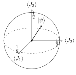
Figure 2: Bloch sphere. Any states of spin $1/2$ is specified as a point $(\langle J_{1}\rangle,\,\langle J_{2}\rangle,\,\langle J_{3}\rangle)$.

3.2 Examples

In this subsection, we look at examples of quasi-joint-probability distributions of the $x$ and $y$ components of spin $1/2$ for two-state quantum systems. First, the exponential functions of $J_{1}$ and $J_{2}$ of spin $1/2$ are given by

$$e^{-isJ_{1}}=\begin{pmatrix}\cos\frac{s}{2}&-i\sin\frac{s}{2}\\ -i\sin\frac{s}{2}&\cos\frac{s}{2}\end{pmatrix},$$ (35)

$$e^{-itJ_{2}}=\begin{pmatrix}\cos\frac{t}{2}&-\sin\frac{t}{2}\\ \sin\frac{t}{2}&\cos\frac{t}{2}\end{pmatrix}.$$ (36)

Then, some of the hashed operators are found as follows:

$$\hat{\#}^{\mathrm{K}}_{J_{1},J_{2}}(s,t)\coloneqq e^{-isJ_{1}}e^{-itJ_{2}}=\begin{pmatrix}\cos\frac{s}{2}\cos\frac{t}{2}-i\sin\frac{s}{2}\sin\frac{t}{2}&-\cos\frac{s}{2}\sin\frac{t}{2}-i\sin\frac{s}{2}\cos\frac{t}{2}\\ \cos\frac{s}{2}\sin\frac{t}{2}-i\sin\frac{s}{2}\cos\frac{t}{2}&\cos\frac{s}{2}\cos\frac{t}{2}+i\sin\frac{s}{2}\sin\frac{t}{2}\end{pmatrix},$$ (37)

$$\hat{\#}^{\mathrm{S}_{1/2}}_{J_{1},J_{2}}(s,t)\coloneqq e^{-i\frac{s}{2}J_{1}}e^{-itJ_{2}}e^{-i\frac{s}{2}J_{1}}=\begin{pmatrix}\cos\frac{s}{2}\cos\frac{t}{2}&-\sin\frac{t}{2}-i\sin\frac{s}{2}\cos\frac{t}{2}\\ \sin\frac{t}{2}-i\sin\frac{s}{2}\cos\frac{t}{2}&\cos\frac{s}{2}\cos\frac{t}{2}\end{pmatrix},$$ (38)

$$\hat{\#}^{\mathrm{M}_{0}}_{J_{1},J_{2}}(s,t) \coloneqq\frac{1}{2}(e^{-isJ_{1}}e^{-itJ_{2}}+e^{-itJ_{2}}e^{-isJ_{1}})$$

$$=\begin{pmatrix}\cos\frac{s}{2}\cos\frac{t}{2}&-\cos\frac{s}{2}\sin\frac{t}{2}-i\sin\frac{s}{2}\cos\frac{t}{2}\\ \cos\frac{s}{2}\sin\frac{t}{2}-i\sin\frac{s}{2}\cos\frac{t}{2}&\cos\frac{s}{2}\cos\frac{t}{2}\end{pmatrix},$$ (39)

$$\hat{\#}^{\mathrm{W}}_{J_{1},J_{2}}(s,t) \coloneqq e^{-i(sJ_{1}+tJ_{2})}$$

$$=\begin{pmatrix}\cos\sqrt{(\frac{s}{2})^{2}+(\frac{t}{2})^{2}}&-i\sqrt{\frac{(\frac{s}{2})-i(\frac{t}{2})}{(\frac{s}{2})+i(\frac{t}{2})}}\sin\sqrt{(\frac{s}{2})^{2}+(\frac{t}{2})^{2}}\\ -i\sqrt{\frac{(\frac{s}{2})+i(\frac{t}{2})}{(\frac{s}{2})-i(\frac{t}{2})}}\sin\sqrt{(\frac{s}{2})^{2}+(\frac{t}{2})^{2}}&\cos\sqrt{(\frac{s}{2})^{2}+(\frac{t}{2})^{2}}\end{pmatrix},$$ (40)

$$\hat{\#}^{\mathrm{B}}_{J_{1},J_{2}}(s,t) \coloneqq\frac{1}{2}\int_{-1}^{1}e^{-i\frac{1-k}{2}sJ_{1}}e^{-itJ_{2}}e^{-i\frac{1+k}{2}sJ_{1}}\,\mathrm{d}k$$

$$=\begin{pmatrix}\cos\frac{s}{2}\cos\frac{t}{2}&\frac{\sin\frac{s}{2}}{\frac{s}{2}}\sin\frac{t}{2}-i\sin\frac{s}{2}\cos\frac{t}{2}\\ -\frac{\sin\frac{s}{2}}{\frac{s}{2}}\sin\frac{t}{2}-i\sin\frac{s}{2}\cos\frac{t}{2}&\cos\frac{s}{2}\cos\frac{t}{2}\end{pmatrix}.$$ (41)

By using these expressions, we can compute each type of quasi-joint-probability distributions with respect to an arbitrary state.

For example, using Eq. (37) the Kirkwood-Dirac distribution with respect to the $\ket{z+}$ state, which is the eigenstate of the eigenvalue $1/2$ of $J_{3}$, is given by

(42)

seeFig.

LABEL:z+-状態のKirkwood-Dirac分布_図(a)and(b).Inthesameway,theoneforthe$\ket{z-}$state,theeigenstatewitheige