Spin-flavor precession of Dirac neutrinos in dense matter and its potential in core-collapse supernovae

Abstract

We calculate the spin-flavor precession (SFP) of Dirac neutrinos induced by strong magnetic fields and finite neutrino magnetic moments in dense matter. As found in the case of Majorana neutrinos, the SFP of Dirac neutrinos is enhanced by the large magnetic field potential and suppressed by large matter potentials composed of the baryon density and the electron fraction. The SFP is possible irrespective of the large baryon density when the electron fraction is close to 1/3. The diagonal neutrino magnetic moments that are prohibited for Majorana neutrinos enable the spin precession of Dirac neutrinos without any flavor mixing. With supernova hydrodynamics simulation data, we discuss the possibility of the SFP of both Dirac and Majorana neutrinos in core-collapse supernovae. The SFP of Dirac neutrinos occurs at a radius where the electron fraction is 1/3. The required magnetic field of the proto-neutron star for the SFP is a few $10^{14}\,$G at any explosion time. For the Majorana neutrinos, the required magnetic field fluctuates from $10^{13}\,$G to $10^{15}\,$G. Such a fluctuation of the magnetic field is more sensitive to the numerical scheme of the neutrino transport in the supernova simulation.

I Introduction

Dirac versus Majorana nature remains one of biggest questions of neutrino physics. During the last several decades numerous experimental and theoretical efforts were directed to answer this question [1]. Neutrinoless double beta ($0\nu\beta\beta$) decay is a promising probe into Majorana neutrinos and lower limits for the decay half-life on various nuclei were continuously updated by many experiments [2]. Usual neutrino oscillation experiments can not distinguish between Dirac and Majorana neutrinos because the flavor conversions in vacuum and matter are associated with the differences of the squares of neutrino masses, not the indivudual masses. These experiments are not sensitive to the Majorana phases either [3]. On the other hand, the coupling of stellar magnetic field and finite neutrino magnetic moments potentially induces the spin-flavor precession (SFP) between left-handed and right-handed neutrinos in astrophysical sites [4, 5, 6]. Such a SFP is completely different from usual flavor conversions conserving the neutrino chirality and its properties are sensitive to Dirac versus Majorana natures.

Recent experiments (e.g., XENONnT [7], CONUS [8], Dresden-II reactor and COHERENT [9], and XMASS-I [10]) constrained the value of neutrino magnetic moment. Among them, the XENONnT experiment gives the most stringent upper limit, $\mu_{\nu}<6.4\times 10^{-12}\mu_{B}$ ($90\%$ C.L.) [7], where $\mu_{B}$ is the Bohr magneton. In addition to the terrestrial experiments, the value of the neutrino magnetic moment can be constrained from the thermal evolution of astronomical phenomena [11, 12, 13, 14, 15]. Currently, neutrino energy loss in globular clusters imposes on the most stringent value, $\mu_{\nu}<1.2\times 10^{-12}\mu_{B}$ [12].

A strong magnetic field larger than $10^{12}$ G is possible in explosive astrophysical sites such as core-collapse supernovae and neutron star mergers (see [16, 17, 18, 19, 20, 21, 22, 23, 24, 25, 26, 27, 28] and the references therein). Large numbers of neutrinos produced there potentially contain information of the magnetic field effects on neutrino oscillations. We note that the neutrino flux from astrophysical sites can be affected by even small intergalactic and interstellar magnetic fields (nG–$\mu$G) [29, 30].

Currently operational neutrino observatories can detect of the order of $10^{4}$ neutrino events from a core-collapse supernova in the Galaxy [31]. Such high statistical neutrino signals enable the investigation on neutrino oscillations inside the star [32, 33, 34, 35]. Furthermore, the nucleosynthesis of heavy nuclei induced by neutrino absorption such as the $\nu p$ process [36, 37, 38, 39] and $\nu$ process [40, 41, 42] is sensitive to large neutrino fluxes near the proto-neutron star (PNS). Therefore, observable quantities such as solar abundances and elemental abundances of heavy nuclei leave clues to the supernova neutrino [38, 39].

It is predicted that neutrino oscillations in core-collapse supernovae are affected by the coherent forward scatterings of neutrinos with background matter and neutrinos themselves [43]. Charged current interactions of neutrinos with background electrons induce the Mikheyev–Smirnov–Wolfenstein (MSW) matter effect [44, 45]. The neutrino-neutrino interactions cause a nonlinear potential in the neutrino Hamiltonian [46, 47, 48, 49, 50, 51, 52, 53, 54, 55] and give various properties of neutrino many-body system that are vigorously investigated such as the neutrino fast flavor instability [56] and many-body nature of collective neutrino oscillation beyond the mean-field [57, 58].

The SFP is affected by these potentials in core-collapse supernovae. The resonant spin-flavor (RSF) conversion occurs resonantly like the MSW effect at the resonance density in core-collapse supernovae [4, 59, 60, 61, 62, 63, 64, 65, 66, 67, 68, 69]. Near the PNS, the neutrino-neutrino interactions are no longer negligible and contribute to neutrino–antineutrino oscillations of Majorana neutrinos [70, 71, 72, 73]. Majorana neutrinos can reach flavor equilibrium in the short scale determined by the strength of magnetic field potential [72, 73]. Such an equilibration phenomenon is induced by the coupling of matter potentials with the magnetic field potential and sensitive to the values of both the baryon density and the electron fraction of the supernova material. The neutrino–antineutrino oscillations can occur even with high baryon density if the electron fraction is close to $0.5$ [73]. In our previous study (hereafter, Ref. [73] is denoted as ST21), we only focused on the equilibration of Majorana neutrinos. However, the SFP should also be possible for Dirac neutrinos.

In this paper, we study the SFP of Dirac neutrinos in dense matter following a similar framework for Majorana neutrinos in ST21[73]. We reveal the mechanism of equilibration of Dirac neutrinos and derive a necessary condition of the SFP in dense matter. Then, we investigate the possibility of SFP of both Dirac and Majorana neutrinos in core-collapse supernovae and discuss the difference between both types of neutrinos.

II Methods

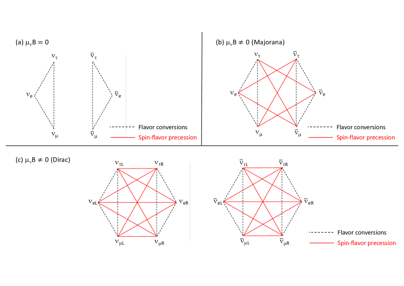
Figure 1: An overview of the magnetic field effect on neutrino oscillations. (a) the case without the magnetic field effect. The dashed black line shows ordinary flavor conversions in both neutrino and antineutrino sectors. (b) the case with the magnetic field effect on Majorana neutrinos. The solid red line shows the SFP induced by the finite neutrino magnetic moment and the magnetic field. (c) the magnetic field effect on Dirac neutrinos. The neutrinos and antineutrinos are decoupled with each other. $\nu_{\alpha L}$ and $\bar{\nu}_{\alpha R}(\alpha=e,\mu,\tau)$ correspond to active left-handed neutrinos ($\nu_{\alpha}$) and right-handed antineutrinos ($\bar{\nu}_{\alpha}$) in (a) and (b).

Figure 1 gives an overview of standard neutrino flavor oscillations as well as the SFP. In the absence of a magnetic field or a neutrino magnetic moment ($\mu_{\nu}B=0$), there is no spin precession among the left- and right-handed neutrinos and the only separate flavor conversions occur in the neutrino and the antineutrino sectors as illustrated in Fig. 1(a). When both the neutrino magnetic moment and magnetic field are finite ($\mu_{\nu}B\neq 0$), then the SFP occurs together with usual flavor conversions. For the Majorana neutrinos in Fig. 1(b), the right-handed neutrino corresponds to the antineutrino and the SFP convert neutrinos into antineutrinos and vice versa. The spin precession without changing the flavor such as $\nu_{\alpha}\leftrightarrow\bar{\nu}_{\alpha}(\alpha=e,\mu,\tau)$ is prohibited due to the vanishing diagonal magnetic moments for Majorana neutrinos. With a strong magnetic field, Majorana neutrinos can reach an equilibrium of neutrino–antineutrino oscillations [72, 73]. On the other hand, for the Dirac neutrinos, the neutrino and antineutrino sectors are decoupled as in Fig. 1(c), and the spin precession such as $\nu_{\alpha L}\leftrightarrow\nu_{\alpha R}$ is allowed due to the existence of diagonal magnetic moments. The magnetic field effect on neutrino oscillations is significantly different for Majorana and Dirac neutrinos although there is no difference in ordinary flavor conversions.

We study the magnetic field effect on Dirac neutrino oscillations as in Fig. 1(c) following our previous work on Majorana neutrino oscillations (ST21[73]). We focus only on conversions of left-handed and right-handed neutrinos and ignore the effect of neutrino-neutrino interactions. We consider a single neutrino energy, $E=1\,$MeV with an emission angle $\theta\in[-\frac{\pi}{3},\frac{\pi}{3}]$ at a radius $r$ (This projection angle $\theta$ should not be confused with the neutrino mixing angles which carry indices, i.e. $\theta_{12}$.). The neutrino conversions are calculated with the Liouville von Neumann equation [72, 73],

$$\cos\theta\frac{\partial}{\partial r}D=-i[H,D],$$ (1)

where $D$ and $H$ are the neutrino density matrix and Hamiltonian for $\nu_{L}$ and $\nu_{R}$,

$$D = \left(\begin{array}[]{cc}\rho_{L\theta}&X_{\theta}\\ X_{\theta}^{\dagger}&\rho_{R\theta}\end{array}\right),$$ (4)

$$H = \left(\begin{array}[]{cc}H_{L}&V_{\mathrm{mag}}\\ V_{\mathrm{mag}}^{\dagger}&H_{R}\end{array}\right),$$ (7)

$$H_{L}=\Omega(E)+V_{\mathrm{mat}},$$ (8)

where $\rho_{L\theta}$ and $\rho_{R\theta}$ are $3\times 3$ density matrices of left- and right-handed neutrinos emitted with the angle $\theta$, and $X_{\theta}$ is a correlation between $\nu_{L}$ and $\nu_{R}$. We use the vacuum term of left-handed neutrinos $\Omega(E)$ in Eq. (8) of Ref. [37] with neutrino mixing parameters, $\{\Delta m_{21}^{2},\Delta m_{32}^{2},\theta_{12},\theta_{13},\theta_{23}\}$, where we assume normal neutrino mass hierarchy ($\Delta m_{32}^{2}>0$) and no CP phase ($\delta_{\rm CP}=0$). The Hamiltonian of right-handed neutrinos is given by [4],

$$H_{R}=\frac{\Delta m_{21}^{2}}{6E}\left(\begin{array}[]{ccc}-2&0&0\\ 0&1&0\\ 0&0&1\end{array}\right)+\frac{\Delta m_{32}^{2}}{6E}\left(\begin{array}[]{ccc}-1&0&0\\ 0&-1&0\\ 0&0&2\end{array}\right),\$$ (9)

where we ignore neutrino mixings and any interaction of the right-handed neutrinos with background particles. The matter potential in Eq. (8) is described by ST21[73],

$$V_{\mathrm{mat}} = -\frac{\lambda_{n}}{2}I_{3\times 3}+\lambda_{e}\left(\begin{array}[]{ccc}1&0&0\\ 0&0&0\\ 0&0&0\end{array}\right),$$ (13)

$$\lambda_{e} = \sqrt{2}G_{F}\rho_{\mathrm{b}}N_{A}Y_{e},$$ (14)

$$\lambda_{n} = \sqrt{2}G_{F}\rho_{\mathrm{b}}N_{A}(1-Y_{e}),$$ (15)

where $G_{F}$ is the Fermi coupling constant, $\rho_{\mathrm{b}}$ is the baryon density, $N_{A}$ is the Avogadro number, $Y_{e}$ is the electron fraction, and $I_{3\times 3}$ is the $3\times 3$ identity matrix. $V_{\mathrm{mag}}$ in Eq. (7) is the potential associated with the coupling of neutrino magnetic moments with the magnetic field,

$$V_{\mathrm{mag}}=B_{T}\left(\begin{array}[]{ccc}\mu_{ee}&\mu_{e\mu}&\mu_{e\tau}\\ \mu_{\mu e}&\mu_{\mu\mu}&\mu_{\mu\tau}\\ \mu_{\tau e}&\mu_{\tau\mu}&\mu_{\tau\tau}\end{array}\right),$$ (19)

where $B_{T}$ is a transverse magnetic field perpendicular to the direction of neutrino emission and $\mu_{\alpha\beta}(\alpha,\beta=e,\mu,\tau)$ are neutrino magnetic moments. This magnetic field potential is in the non-diagonal component of Eq. (7) inducing the mixing between left- and right-handed neutrinos. The diagonal neutrino magnetic moments $\mu_{\alpha\alpha}(\alpha=e,\mu,\tau)$ that are ignored in Majorana neutrinos need to be considered in Dirac neutrinos. Here we assume flavor-independent diagonal terms and anti-symmetric non-diagonal terms in Eq. (19),

$$V_{\mathrm{mag}}=\Omega_{\mathrm{d}}I_{3\times 3}+\Omega_{\mathrm{nd}}\left(\begin{array}[]{ccc}0&1&1\\ -1&0&1\\ -1&-1&0\end{array}\right),$$ (23)

where $\Omega_{\mathrm{d}}$ and $\Omega_{\mathrm{nd}}$ characterize the strengths of diagonal and non-diagonal neutrino magnetic moments.

III Results and Discussions

III.1 Non-diagonal magnetic field potential $\Omega_{\mathrm{nd}}$

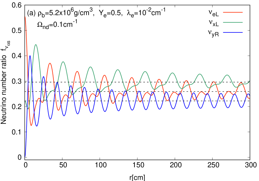
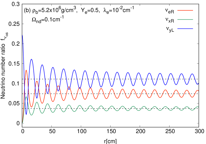
Figure 2: (a) The SFP of Dirac neutrinos with the non-diagonal term $\Omega_{\mathrm{nd}}=0.1\,\mathrm{cm}^{-1}$ in Eq. (23) for $\lambda_{e}=0.1\Omega_{\mathrm{nd}}$ and $Y_{e}=0.5$ in the $\nu_{eL}$–$\nu_{xL}$–$\nu_{yR}$ sector. The dashed lines show equilibrium values $(n_{\nu_{e}}+n_{\nu_{x}})/3n_{\nu}=7/27$, $(2n_{\nu_{e}}+3n_{\nu_{x}})/6n_{\nu}=8/27$, and $(2n_{\nu_{e}}+n_{\nu_{x}})/6n_{\nu}=2/9$. (b) The result of the $\nu_{eR}$–$\nu_{xR}$–$\nu_{yL}$ sector. The dashed lines correspond to the values of $n_{\nu_{x}}/3n_{\nu}=2/27$, $n_{\nu_{x}}/6n_{\nu}=1/27$, and $n_{\nu_{x}}/2n_{\nu}=1/9$.

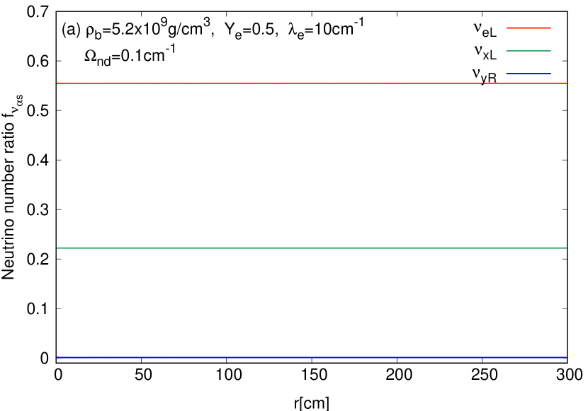
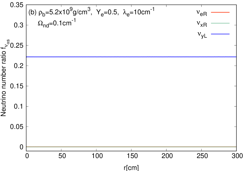
Figure 3: The SFP of Dirac neutrinos with the non-diagonal term $\Omega_{\mathrm{nd}}=0.1\,\mathrm{cm}^{-1}$ for $\lambda_{e}=10^{2}\Omega_{\mathrm{nd}}$ and $Y_{e}=0.5$ both in (a) $\nu_{eL}$–$\nu_{xL}$–$\nu_{yR}$ and (b) $\nu_{eR}$–$\nu_{xR}$–$\nu_{yL}$ sector.

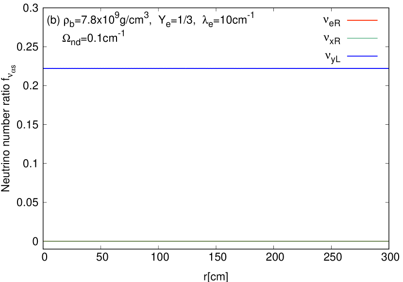
Figure 4: The SFP of Dirac neutrinos with the non-diagonal term $\Omega_{\mathrm{nd}}=0.1\,\mathrm{cm}^{-1}$ for $\lambda_{e}=10^{2}\Omega_{\mathrm{nd}}$ and $Y_{e}=1/3$ both in (a) $\nu_{eL}$–$\nu_{xL}$–$\nu_{yR}$ and (b) $\nu_{eR}$–$\nu_{xR}$–$\nu_{yL}$ sector. The dashed line in (a) shows $n_{\nu_{e}}/2n_{\nu}=5/18$.

We calculate the magnetic field effect on Dirac neutrino oscillations by setting the initial condition of diagonal terms of left-handed neutrinos, $(\rho_{L\theta})_{\alpha\alpha}=n_{\nu_{\alpha}}/n_{\nu}\,(\alpha=e,\mu,\tau)$ where $n_{\nu}=\sum_{\alpha=e,\mu,\tau}n_{\nu_{\alpha}}$ and $n_{\nu_{x}}/n_{\nu_{e}}=0.4\,(x=\mu,\tau)$. All of the other components in Eq. (4) are set to zero at $r=0$. In Sec. III.1, we fix the strength of the non-diagonal magnetic field potential $\Omega_{\mathrm{nd}}=(\mu_{\nu}/10^{-12}\,\mu_{B})(B_{T}/3.4\times 10^{14}\,\mathrm{G})=0.1\,\mathrm{cm}^{-1}$ and ignore the diagonal term ($\Omega_{\mathrm{d}}=0\,\mathrm{cm}^{-1}$). In order to study the sensitivity of matter potential in Eq. (13), we change the values of electron fraction $Y_{e}$ and the baryon density given by $\rho_{\mathrm{b}}=5.2\times 10^{6}\,\mathrm{g}/\mathrm{cm}^{3}(Y_{e}/0.5)^{-1}(\lambda_{e}/10^{-2}\,\mathrm{cm}^{-1})$.

Low density case

Figure 2 shows the result of neutrino number ratios in the fixed values of $\rho_{\mathrm{b}}=5.2\times 10^{6\,}\mathrm{g}/\mathrm{cm}^{3}$ and $Y_{e}=0.5$, which corresponds to $\lambda_{e}=0.1\Omega_{\mathrm{nd}}$. Such ratios of Dirac neutrinos $\nu_{\alpha s}(\alpha=e,x,y,s=L,R)$ are obtained by averaging the diagonal components of neutrino density matrices,

$$f_{\nu_{\alpha s}} = \frac{3}{2\pi}\int^{\frac{\pi}{3}}_{\frac{\pi}{3}}\mathrm{d}\theta\ (\rho_{s\theta})_{\alpha\alpha},$$ (24)

where $\nu_{xs}$ and $\nu_{ys}$ are eigenstates in a rotated frame described by a linear combination of flavors $\mu$ and $\tau$ [74]. The magnetic field potential is a dominant term in neutrino Hamiltonian and SFPs in both $\nu_{eL}-\nu_{xL}-\nu_{yR}$ and $\nu_{eR}-\nu_{xR}-\nu_{yL}$ sectors are prominent. The vacuum frequencies associated with $\Delta m_{21}^{2}$ and $\Delta m_{32}^{2}$ are negligible compared with $\Omega_{\mathrm{nd}}$. Therefore, the values of $f_{\nu_{eL}}+f_{\nu_{xL}}+f_{\nu_{yR}}$ and $f_{\nu_{eR}}+f_{\nu_{xR}}+f_{\nu_{yL}}$ are almost constant. The neutrino ratios are oscillating around the dashed lines and such equilibrium values are derived in Appendix A.1.

The SFP discussed in Fig. 2–5 is almost independent of the vacuum term and the neutrino mass hierarchy. We remark that the vacuum frequencies can contribute to the SFP and the hierarchy dependence becomes prominent when the magnetic field potential is comparable with the vacuum frequencies and other potentials in the Hamiltonian are negligible. We mention such a hierarchy difference in core-collapse supernovae in Sec. III.2.

High density case

Figure 3 shows the result in the case of $\lambda_{e}=10^{2}\Omega_{\mathrm{nd}}$ with $\rho_{\mathrm{b}}=5.2\times 10^{9\,}\mathrm{g}/\mathrm{cm}^{3}$ and $Y_{e}=0.5$. The numerical setup for Fig. 3 is the same as that of Fig. 2 except for the value of $\rho_{b}$. All of the calculated neutrino number ratios are constant ($f_{\nu_{eL}}=5/9,f_{\nu_{xL}}=f_{\nu_{yL}}=2/9,f_{\nu_{eR}}=f_{\nu_{xR}}=f_{\nu_{yR}}=0$) in Fig. 3 and any SFP and usual flavor conversions are negligible. Such suppression due to the large matter potential is also confirmed in Majorana neutrinos [73]. In general, the magnetic field potential should be dominant among the potentials in the neutrino Hamiltonian for the significant SFP.

Case for $Y_{e}\sim 1/3$

The matter potentials $\lambda_{e}$ and $\lambda_{n}$ depends on both the baryon density and the electron fraction. Therefore, the matter suppression in Fig. 3 is sensitive to the value of the electron fraction and the SFP is possible in some specific value of the electron fraction even in the large baryon density. Figure 4 shows the result in $\lambda_{e}=10^{2}\Omega_{\mathrm{nd}}$ with $\rho_{\mathrm{b}}=7.8\times 10^{9}\,\mathrm{g}/\mathrm{cm}^{3}$ and $Y_{e}=1/3$. Evolutions of $\nu_{xL},\nu_{yL},\nu_{eR},$ and $\nu_{xR}$ are negligible by the large matter potential $\lambda_{n}$. On the other hand, the SFP between $\nu_{eL}$ and $\nu_{yR}$ can avoid matter suppression. Such a SFP occurs where $|\lambda_{e}-\lambda_{n}/2|\ll\Omega_{\mathrm{nd}}$ is satisfied. $Y_{e}=1/3$ satisfies this condition irrespective of the value of $\rho_{b}$. We remark that, for Majorana neutrinos, a similar SFP independent of the value of $\rho_{b}$ occurs around $Y_{e}\sim 0.5$ where $|\lambda_{e}-\lambda_{n}|\ll\Omega_{\mathrm{nd}}$ is satisfied [73]. The mechanism of such $\rho_{\mathrm{b}}$ independent SFP of Dirac neutrinos at $Y_{e}=1/3$ is derived in Appendix A.3. More detail on the difference between Dirac and Majorana neutrinos is discussed in Appendix B.

Almost the same discussion is possible for the right-handed antineutrinos by exchanging the sign of matter potential $\lambda_{e(n)}\to-\lambda_{e(n)}$. Then, the equilibrium values of active neutrinos ($f_{\nu_{\alpha}}^{\mathrm{eq}},f_{\bar{\nu}_{\alpha}}^{\mathrm{eq}}(\alpha=e,x,y)$) as in the dashed lines of Figs. 2 and 4 are connected with initial neutrino ratios ($f_{\nu_{\alpha}}^{i},f_{\bar{\nu}_{\alpha}}^{i}$) through a transition matrix $U_{\mathrm{mag}}^{D}$,

$$\left(\begin{array}[]{c}F^{\mathrm{eq}}_{\nu}\\ F^{\mathrm{eq}}_{\bar{\nu}}\end{array}\right)=\left(\begin{array}[]{cc}U_{\mathrm{mag}}^{D}&0\\ 0&U_{\mathrm{mag}}^{D}\end{array}\right)\left(\begin{array}[]{c}F^{\mathrm{i}}_{\nu}\\ F^{\mathrm{i}}_{\bar{\nu}}\end{array}\right),$$ (25)

$$F^{i(\mathrm{eq})}_{\nu} = \left(\begin{array}[]{c}f_{\nu_{e}}^{i(\mathrm{eq})}\\ f_{\nu_{x}}^{i(\mathrm{eq})}\\ f_{\nu_{y}}^{i(\mathrm{eq})}\end{array}\right),$$ (29)

$$F^{i(\mathrm{eq})}_{\bar{\nu}} = \left(\begin{array}[]{c}f_{\bar{\nu}_{e}}^{i(\mathrm{eq})}\\ f_{\bar{\nu}_{x}}^{i(\mathrm{eq})}\\ f_{\bar{\nu}_{y}}^{i(\mathrm{eq})}\end{array}\right),$$ (33)

where $U_{\mathrm{mag}}^{D}$ is a $3\times 3$ transition matrix. The values of the $U_{\mathrm{mag}}^{D}$ for three different extreme cases of neutrino potentials are shown in Table 1. Figs. 2–4 correspond to the cases of (1)–(3) in the table. Our demonstration assumes that both the matter and the magnetic field potentials are sufficiently large compared with the vacuum Hamiltonian. For the case of (2) in Table 1, the SFP is suppressed and the $U_{\mathrm{mag}}^{D}$ is equivalent to the $3\times 3$ identity matrix. For the case of (1) and (3), the summation of $f_{\nu_{\alpha}}^{\mathrm{eq}}(\alpha=e,x,y)$ is less than that of $f_{\nu_{\alpha}}^{i}$ due to the coupling with the right-handed neutrinos. Such a reduction of ratios of left-handed neutrinos is confirmed in antineutrinos too.

As shown in Eq. (25), the neutrino and antineutrino sectors are decoupled from each other for Dirac neutrinos due to the decoupling as in Fig. 1(c). On the other hand, for Majorana neutrinos, the SFP occurs between neutrinos and antineutrinos as in Fig. 1(b). The equilibrium values of number ratios in three extreme cases are summarized in Eq. (85) and Table 2 in Appendix B. Since the total number of active neutrinos $(\sum_{\alpha=e,x,y}f_{\nu_{\alpha}}^{\mathrm{eq}}+f_{\bar{\nu}_{\alpha}}^{\mathrm{eq}})$ is conserved through the SFP in Majorana neutrinos, the reduced neutrino flux could be a prominent feature that distinguishes both Dirac and Majorana neutrinos.

Case	$U_{\mathrm{mag}}^{D}$
(1) $|\lambda_{e}-\lambda_{n}/2|,\lambda_{n}\ll\Omega_{\mathrm{nd}}$	$\left(\begin{array}[]{ccc}\frac{1}{3}&\frac{1}{3}&0\\ \frac{1}{3}&\frac{1}{2}&0\\ 0&0&\frac{1}{2}\end{array}\right)$
(2) $|\lambda_{e}-\lambda_{n}/2|,\lambda_{n}\gg\Omega_{\mathrm{nd}}$	$\left(\begin{array}[]{ccc}1&0&0\\ 0&1&0\\ 0&0&1\end{array}\right)$
(3) $|\lambda_{e}-\lambda_{n}/2|\ll\Omega_{\mathrm{nd}},\lambda_{n}\gg\Omega_{\mathrm{nd}}$	$\left(\begin{array}[]{ccc}\frac{1}{2}&0&0\\ 0&1&0\\ 0&0&1\end{array}\right)$

Table 1: The transition matrix $U_{\mathrm{mag}}^{D}$ in Eq. (25) for Dirac neutrinos with the nondiagonal magnetic field potential $\Omega_{\mathrm{nd}}$ in Eq. (23) in three extreme cases of the matter and the magnetic field potentials. Case (3) is satisfied if $Y_{e}\sim 1/3$.

III.2 Diagonal magnetic field potential $\Omega_{\mathrm{d}}$

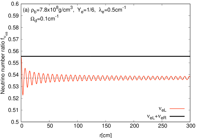
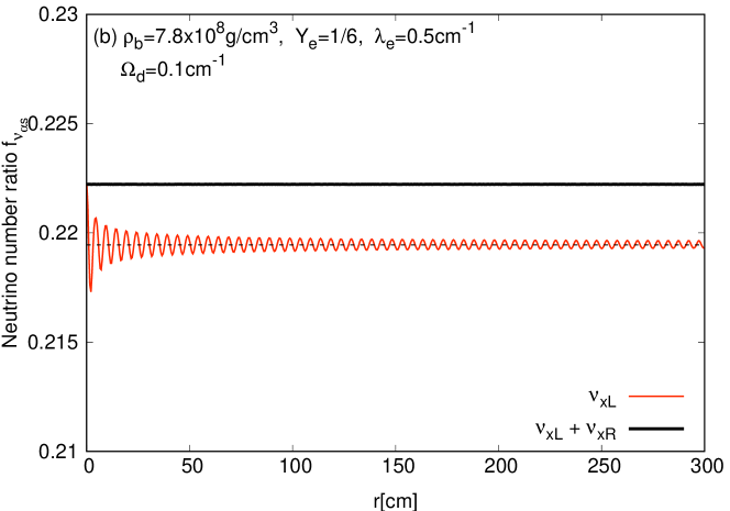
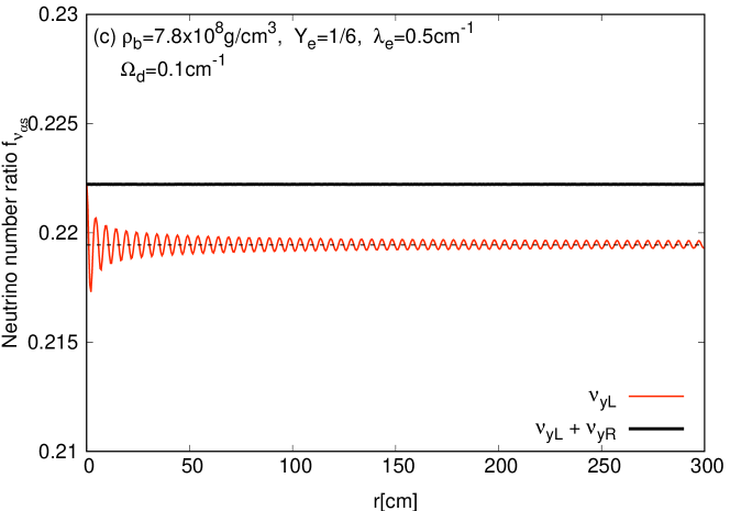
Figure 5: The SFP of Dirac neutrinos with the diagonal term $\Omega_{\mathrm{d}}=0.1\,\mathrm{cm}^{-1}$ in Eq. (23) for $\lambda_{e}=5\Omega_{\mathrm{d}}$ and $Y_{e}=1/6$ in (a) $\nu_{eL}$–$\nu_{eR}$, (b) $\nu_{xL}$–$\nu_{xR}$, and (c) $\nu_{yL}$–$\nu_{yR}$ sector. The dashed lines correpond to Eqs. (34) and (35).

We discuss the SFP of Dirac neutrinos induced by the diagonal neutrino magnetic moment. We employ the same initial condition for the neutrino density matrix as Sec. III.1 and fix the strength of magnetic field potential as $\Omega_{\mathrm{d}}=0.1\,\mathrm{cm}^{-1}$ and $\Omega_{\mathrm{nd}}=0\,\mathrm{cm}^{-1}$ in Eq. (23).

Figure 5 shows the result of the SFP induced by diagonal magnetic field potential $\Omega_{\mathrm{d}}$ with $\rho_{\mathrm{b}}=7.8\times 10^{8\,}\mathrm{g}/\mathrm{cm}^{3}$ and $Y_{e}=1/6$ resulting in $\lambda_{e}=5\Omega_{\mathrm{d}}$. The red lines are evolutions of $f_{\nu_{\alpha L}}(\alpha=e,x,y)$ and the black lines are the summations of $f_{\nu_{\alpha L}}+f_{\nu_{\alpha R}}$ that are almost constant in the calculation. Such constant black lines suggest that the SFPs occur in the same flavors $\nu_{\alpha L}$–$\nu_{\alpha R}(\alpha=e,x,y)$ and are decoupled with each other. The dynamics of $\nu_{\alpha L}$–$\nu_{\alpha R}$ can be solved in the same way as usual two flavor conversions. The result of Fig. 5(a) is consistent with the conversion $\nu_{eL}$–$\nu_{eR}$ in Ref. [4]. The equilibrium values of the left-handed neutrinos (dashed lines) are given by

$$f_{\nu_{e}}^{\mathrm{eq}} = f_{\nu_{e}}^{i}\left\{1-\frac{2\Omega_{\mathrm{d}}^{2}}{(\lambda_{e}-\frac{\lambda_{n}}{2})^{2}+4\Omega_{\mathrm{d}}^{2}}\right\},$$ (34)

$$f_{\nu_{x(y)}}^{\mathrm{eq}} = f_{\nu_{x(y)}}^{i}\left\{1-\frac{2\Omega_{\mathrm{d}}^{2}}{(\frac{\lambda_{n}}{2})^{2}+4\Omega_{\mathrm{d}}^{2}}\right\}.$$ (35)

Similar relations are derived in the antineutrino sector. These equations show that conversions become maximum when the magnetic field potential is dominant $|\lambda_{e}-\lambda_{n}/2|,\lambda_{n}\ll\Omega_{\mathrm{d}}$. Conversely, any SFP is negligible when the matter potentials are large $|\lambda_{e}-\lambda_{n}/2|,\lambda_{n}\gg\Omega_{\mathrm{d}}$. The matter suppression does not occur in $\nu_{eL}$–$\nu_{eR}$ even in the large baryon density when the electron fraction is close to $1/3$ because of $|\lambda_{e}-\lambda_{n}/2|\sim 0$. Our demonstration indicates that, in both non-diagonal and diagonal cases, the strong magnetic field potentials larger than $|\lambda_{e}-\lambda_{n}/2|$ are necessary for the significant SFP of Dirac neutrinos.

III.3 Dirac vs Majorana in core-collapse supernovae

We investigate the possibility of the SFP of both Dirac and Majorana neutrinos in core-collapse supernovae with neutrino spectra and matter profiles obtained in a neutrino radiation-hydrodynamic simulation of $11.2\,M_{\odot}$ progenitor model used in the demonstration for the Majorana neutrinos in ST21[73].

As discussed in previous sections, the strength of magnetic field potential $\Omega_{\mathrm{mag}}=\mu_{\nu}B_{T}$ should be larger than $|\lambda_{e}-\lambda_{n}/2|(|\lambda_{e}-\lambda_{n}|)$ for the significant SFP of the Dirac (Majorana) neutrinos. To study the possibility of the SFP in core-collapse supernovae, we need to compare the magnetic field potential with other potentials in the neutrino Hamiltonian.

Near the proto-neutron star (PNS) in core-collapse supernovae ($r\sim 10$ km), the neutrino-neutrino interaction could induce a non-negligible potential in the neutrino Hamiltonian. The strength of the neutrino-neutrino interactions at the radius from the center $r$ could be estimated as ST21[73],

$$\begin{split}\zeta=\frac{\sqrt{2}G_{F}}{4\pi R_{\nu}^{2}}\left|\frac{L_{\nu_{e}}}{\langle E_{\nu_{e}}\rangle}-\frac{L_{\bar{\nu}_{e}}}{\langle E_{\bar{\nu}_{e}}\rangle}\right|\left(1-\sqrt{1-\left(\frac{R_{\nu}}{r}\right)^{2}}\right)^{2},\end{split}$$ (36)

where $\langle E_{\nu_{i}}\rangle$ and $L_{\nu_{i}}$ are the mean energy and luminosity of $\nu_{i}(\nu_{i}=\nu_{e},\bar{\nu}_{e})$ on the surface of the PNS ($r=R_{\nu}$). We define the value of $R_{\nu}$ at a radius where the baryon density corresponds to $\rho_{\mathrm{b}}=10^{11}\,\mathrm{g}/\mathrm{cm}^{3}$.

In outer region of supernova matter ($r>10^{3}$ km), the potentials of both matter and neutrino-neutrino interactions decrease and the vacuum Hamiltonian $\Omega(E)$ in Eq. (8) becomes dominant. The strength of the vacuum Hamiltonian in our demonstration could be characterized by the atmospheric vacuum frequency $\omega=|\Delta m_{32}^{2}|/2E$ where $E=10$ MeV is a typical neutrino mean energy in core-collapse supernovae.

The magnetic field potential should be dominant among the potentials in the neutrino Hamiltonian for the significant SFP. Then, the necessary conditions for the SFPs of both Dirac and Majorana neutrinos are given by

$$\Omega_{\mathrm{mag}} \geq \eta$$ (37)

$$\eta = \begin{cases}\mathrm{max}\{\lambda_{D},\zeta,\omega\}&(\mathrm{Dirac})\\ \mathrm{max}\{\lambda_{M},\zeta,\omega\}&(\mathrm{Majorana}),\end{cases}$$ (38)

where $\lambda_{D}=|\lambda_{e}-\lambda_{n}/2|$ and $\lambda_{M}=|\lambda_{e}-\lambda_{n}|$. $\eta$ is the maximum values among the three strengths and the difference between Dirac and Majorana neutrinos appears at $\lambda_{D}$ and $\lambda_{M}$.

For the model of the magnetic field, we use a dipole magnetic field as employed in ST21[73],

$$B_{T}=B_{0}\left(\frac{R_{\nu}}{r}\right)^{3},$$ (39)

where $B_{0}$ is the transverse magnetic field on the surface of PNS ($r=R_{\nu}$). The strength of magnetic field potential $\Omega_{\mathrm{mag}}=\mu_{\nu}B_{T}$ is calculated with a fixed value of the neutrino magnetic moment, $\mu_{\nu}=10^{-12}\mu_{B}$, satisfying the current experimental upper limit [7].

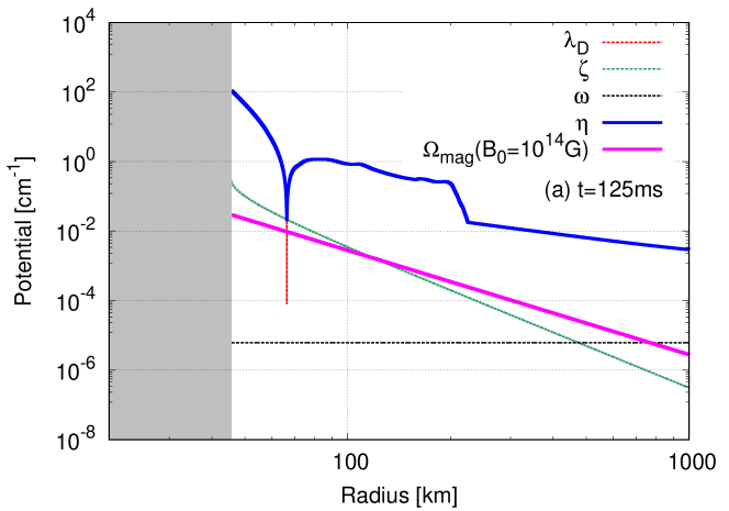
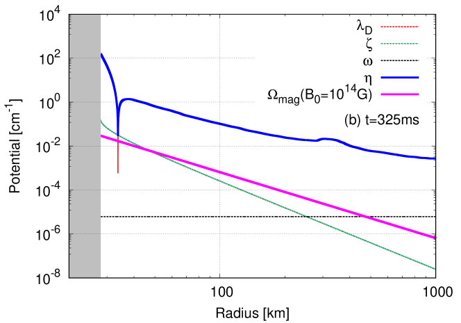
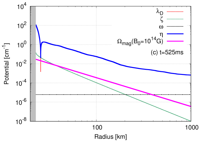
Figure 6: The potentials used for Eqs. (37) and (38) for Dirac neutrinos at different explosion time after postbounce ($t=125,\,325,\,525\,$ms). The shaded region shows the interior of the PNS.

Figure 6 shows the strengths of the potentials and $\eta$ in Eq. (38) for Dirac neutrinos at $t=125,\,325,\,525$ ms after postbounce. The shaded region shows the interior of the PNS. The radius of the boundary corresponds to the PNS radius $R_{\nu}$. The PNS radius becomes smaller as the explosion time has passed due to the shrink of the PNS. In all of the explosion time, the maximum strength $\eta$ (blue line) is given by $\lambda_{D}$ (red line) in $r>R_{\nu}$ except for a peak of $\lambda_{D}\sim 0$ where $Y_{e}=1/3$ and $\eta=\zeta$ (green line) in Eq. (36). Near the surface of PNS, $\lambda_{D}$ is large because of the dense and neutron-rich matter. On the other hand, the neutrino heating increases the value of electron fraction outside the PNS, which results in the point of $\lambda_{D}\sim 0$ within $r<100\,$km. The baryon density decreases monotonously outside this point and the sudden decrease of $\lambda_{D}$ around 200 km in Fig. 6(a) corresponds to the propagating shock front.

The values of $\Omega_{\mathrm{mag}}$ in Fig. 6 (magenta lines) are obtained with the typical magnetic field of magnetars $B_{0}=10^{14}$ G in Eq. (39). The magenta lines can move upwards with large $B_{0}$ keeping the same slope due to the same radial dependence of Eq. (39). The necessary condition in Eq. (37) is satisfied where the magenta lines are larger than the blue lines. The magenta lines in Fig. 6 are always smaller than the blue lines, which indicates that $B_{0}=10^{14}$ G is insufficient to satisfy Eq. (37). For more quantitative discussion, we introduce a minimum magnetic field on the surface of PNS,

$$B_{0,\mathrm{min}}(r)=\frac{r^{3}}{\mu_{\nu}R_{\nu}^{3}}\eta.$$ (40)

Eq. (37) is satisfied at the radius $r$ when $B_{0}>B_{0,\mathrm{min}}(r)$. Figure 7 shows the results of Eq. (40) at different explosion times of Fig. 6. The $B_{0,\mathrm{min}}(r)$ becomes minimum at the point of $\lambda_{D}\sim 0$ at any explosion time. The minimum values are $2.24\times 10^{14},\,1.86\times 10^{14},\,2.23\times 10^{14}\,$G at $t=125,\,325,\,525\,$ms after postbounce. The strong magnetic field $B_{0}>10^{16}\,$G is required for Eq. (37) in regions other than such resonance point.

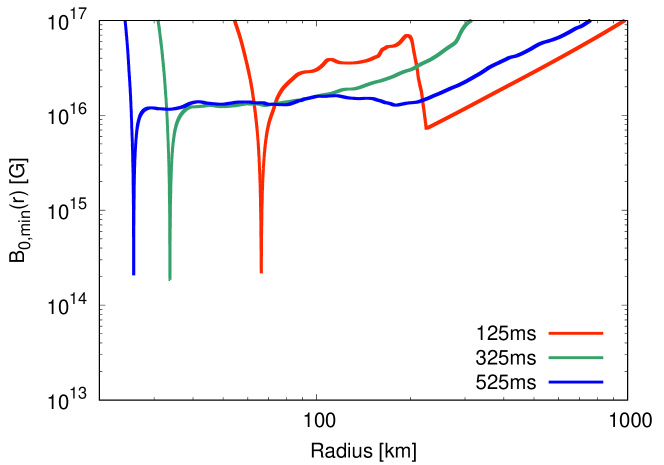
Figure 7: The radial profile of Eq. (40) for Dirac neutrinos.

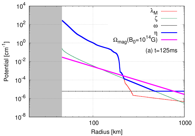
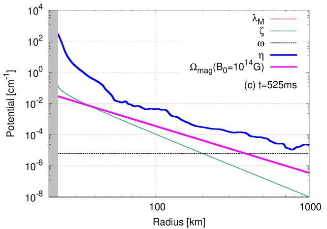
Figure 8: The potentials for the Majorana neutrinos in Eqs. (37) and (38) at $t=125,\,325,\,525\,$ms after postbounce as in Fig. 6.

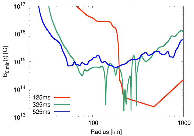
Figure 9: The radial profile of Eq. (40) for Majorana neutrinos.

Figure 8 shows profiles of the potentials for Majorana neutrinos with different time snapshots as in Fig. 6. In Fig. 8 (a), at $t=125\,$ms, the maximum strength $\eta$ (blue line) is equal to $\lambda_{M}$ (red line) near the PNS radius and the $\lambda_{M}$ decreases significantly outside the shock front ($r>$200 km) due to the small baryon density and $Y_{e}\sim 0.5$ in Si layer. Then, the $\eta$ is determined by $\zeta$ (green line) and $\omega$ (black line) in such outer region. The SFP around 800 km would depend on the neutrino mass hierarchy because the $\omega$ becomes maximum and comparable with $\Omega_{\mathrm{mag}}$. Such hierarchy dependence does not appear in Dirac neutrinos within 1000 km because of $\omega<\eta$ at any radius as shown in Fig. 6(a). This does not happen even in $r>1000$ km because of $\omega\gg\Omega_{\mathrm{mag}}$. In Fig. 8 (b), at $t=325\,$ms, there are several peaks of $\lambda_{M}\sim 0$ (red line) where $Y_{e}=0.5$. Such peaks are favorable to satisfy Eq. (37). The small $\lambda_{M}$ enables the crossing of $\Omega_{\mathrm{mag}}$ (magenta lines) and $\eta$ (blue lines) in Figs. 8 (a) and 8 (b). Therefore, $B_{0}=10^{14}$ G is sufficient to satisfy Eq. (37) for Majorana neutrinos. On the other hand, there are no peaks of $\lambda_{M}\sim 0$ at $t=525\,$ms as in Fig. 8 (c) because the electron fraction is not close to $0.5$. Then, there is no crossing of $\Omega_{\mathrm{mag}}$ (magenta line) and $\eta$ (blue line) in this explosion phase.

The result of Eq. (40) for Majorana neutrinos is shown in Fig. 9. As shown in the case of 125 ms (red line), the minimum value is given by $2.34\times 10^{13}\,$G at $r=474\,$km in the Si layer outside the shock wave. After the shock propagation, $B_{0,\mathrm{min}}(r)$ in the shock-heated material becomes small at the point of $Y_{e}=0.5$ and the minimum value at 325 ms (green line) is given by $1.72\times 10^{13}\,$G at $r=222\,$km. There is no point of $Y_{e}=0.5$ at 525 ms and $B_{0,\mathrm{min}}(r)$ is larger than $10^{14}$ G.

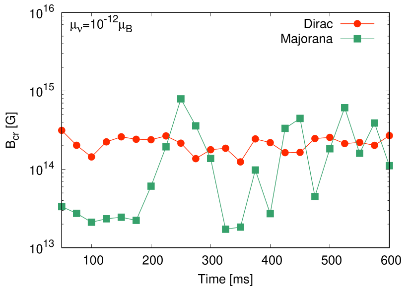
Figure 10: The critical magnetic field on the surface of the PNS in Eq. (41) for both Dirac and Majorana neutrinos.

The minimum value of Eq. (40) outside the PNS radius,

$$B_{\mathrm{cr}}=\min_{r\geq R_{\nu}}\left\{B_{0,\mathrm{min}}(r)\right\},$$ (41)

could be regarded as a critical magnetic field on the surface of PNS for the SFP at the explosion time.

Figure 10 shows the result of Eq. (41) at the different explosion times for both Dirac and Majorana neutrinos. The value for Dirac neutrinos is larger than $10^{14}$ G. As shown in Fig. 7, the $B_{0,\mathrm{min}}(r)$ for Dirac neutrino becomes minimum at the radius of $Y_{e}\sim 1/3$. Such a specific radius appears near the PNS radius inside the shock-heated material. We remark that the supernova matter profiles used in Figs. 6 and 8 are obtained by averaging the contribution from the various directions with the polar angle $\Theta\in[0,\pi]$ of the 2D hydrodynamic simulation. Hence the angular dependence on the profile of $Y_{e}$ is also averaged out in our analysis. In addition, our demonstration implicitly assumes the strength of the dipole magnetic field of the equator of the PNS ($\Theta=\pi/2$) and ignores the dependence of $\sin\Theta$ on Eq. (39) [64]. Such a $\Theta$ dependence implies that the spin precession is less likely to occur in the polar direction ($\Theta\sim 0$) due to the larger critical magnetic field.
As shown in Fig. 10, the value of $B_{\mathrm{cr}}$ for Majorana neutrinos is less than $10^{14}$ G and smaller than those of Dirac neutrinos in $t<200$ ms. In this early explosion phase, as in Fig. 8(a), the value of $\lambda_{M}$ decreases significantly outside the shock front where $\rho_{b}$ is small and $Y_{e}$ is close to $0.5$ due to many $\alpha$ elements, which results in the small $B_{\mathrm{cr}}$. The SFP of Majorana neutrinos is more favorable than those of Dirac neutrinos in the early phase before the shock wave has reached the $\alpha$ elements layer.
While propagating outwards, the shock wave heats the material of outer layers and changes the value of $Y_{e}$. In the later explosion phase ($t\geq 200$ ms), $B_{\mathrm{cr}}$ for Majorana neutrinos fluctuates between $10^{13}$–$10^{15}$ G although the value for Dirac neutrinos is roughly constant. Such fluctuations originated from several peaks of $\lambda_{M}\sim 0$ as in Fig. 8(b) and the absence of the peaks as in Fig. 8(c). The value of $Y_{e}$ is particularly uncertain around $0.5$ and dependent on the neutrino radiation transport scheme used in the supernova hydrodynamic simulation. More elaborate neutrino transport would enable a more detailed analysis of Majorana neutrinos in the later explosion phase.

In this study, we primarily focused on delineating the criteria for SFP, and omitted an elaboration of the anticipated neutrino event rate and spectrum. To predict them, we need to investigate other aspects of neutrino oscillations, especially collective neutrino oscillations. In particular, the implications of fast flavor conversions in supernova environments is actively debated (e.g., [75, 76, 77, 78]). A comprehensive study encompassing both SFP and fast flavor conversions is deferred to future work.

IV Conclusion

We calculate the SFP of Dirac neutrinos induced by the coupling of neutrino magnetic moments and magnetic fields in dense matter. This work is an extension of our previous work for neutrino–antineutrino oscillations of Majorana neutrinos [73]. We demonstrate the SFP of Dirac neutrinos for both diagonal and non-diagonal neutrino magnetic moments. The SFP occurs significantly when the matter potentials are negligible compared with the magnetic field potential. The large baryon density tends to prevent the SFP. However, the SFP is possible in $\nu_{e}$ even with the large baryon density when the electron fraction is close to $1/3$.

Finally, we verify the possibility of the SFP of both Dirac and Majorana neutrinos in core-collapse supernovae based on the necessary condition of the SFP derived from our demonstrations by using simulation data of $11.2\,M_{\odot}$ progenitor model with a fixed value of neutrino magnetic moment $\mu_{\nu}=10^{-12}\mu_{B}$. In the case of Dirac neutrinos, the required magnetic field on the surface of the PNS for the SFP is a few $10^{14}\,$G at any explosion time. The required magnetic field for Majorana neutrinos is a few $10^{13}\,$G in the early explosion phase before the shock reaches the Si layer. On the other hand, in the later explosion phase, the magnetic field fluctuates between $10^{13}$–$10^{15}\,$G, which is sensitive to the scheme of the neutrino transport used in hydrodynamic simulation.

Appendix A Matter suppression with $\Omega_{\mathrm{nd}}$

Following a similar approach as done in ST21[73], we derive the equilibrium values (dashed lines) in Figs. 2 and  4. We solve Eq. (1) with $\theta=0$ assuming the dense matter $H_{L}\sim V_{\mathrm{mat}}$, $H_{R}\sim 0$, and the negligible diagonal neutrino magnetic moment $\Omega_{\mathrm{d}}=0$ in Eq. (23). The term $\theta$ in Eq. (4) is dropped hereafter. Then, the equation of motion in Eq. (1) is decomposed by

$$\partial_{r}\rho_{L} \sim -i[V_{\mathrm{mat}},\rho_{L}]-i(V_{\mathrm{mag}}X^{\dagger}-XV_{\mathrm{mag}}^{\dagger}),$$ (42)

$$\partial_{r}\rho_{R} \sim -i(V_{\mathrm{mag}}^{\dagger}X-X^{\dagger}V_{\mathrm{mag}}),$$ (43)

$$\partial_{r}X \sim -i(V_{\mathrm{mat}}X+V_{\mathrm{mag}}\rho_{R}-\rho_{L}V_{\mathrm{mag}}),$$ (44)

where $\partial_{r}=\partial/\partial_{r}$. The above equations of motion in $e-\mu-\tau$ basis can be described in $e-x-y$ basis through the transformation of matrices such as

$$V_{\mathrm{mat}}^{\prime} = R^{T}(\theta_{23})V_{\mathrm{mat}}R(\theta_{23})$$ (45)

$$= V_{\mathrm{mat}},$$

$$V_{\mathrm{mag}}^{\prime} = R^{T}(\theta_{23})V_{\mathrm{mag}}R(\theta_{23})$$ (49)

$$= \Omega_{\mathrm{nd}}\left(\begin{array}[]{c c c}0&0&\sqrt{2}\\ 0&0&1\\ -\sqrt{2}&-1&0\end{array}\right),$$

$$R(\theta_{23}) = \left(\begin{array}[]{c c c}1&0&0\\ 0&\cos\theta_{23}&\sin\theta_{23}\\ 0&-\sin\theta_{23}&\cos\theta_{23}\end{array}\right),$$ (53)

where $\theta_{23}=\pi/4$. Here we comment that the matrix components of Eq. (A4) in ST21[73] should be corrected as Eq. (49) for a more precise discussion on Majorana neutrinos although the same equilibrium values of neutrino–antineutrino oscillations are derived with Eq. (49). Following the matrix transformation of Eqs. (45)-(53), the evolutions of matrix components of the neutrino density matrices in $e-x-y$ basis are given by

$$\partial_{r}\rho_{Lee} = -2\sqrt{2}\Omega_{\mathrm{nd}}X_{ey,i},$$ (54)

$$\partial_{r}\rho_{Lxx} = -2\Omega_{\mathrm{nd}}X_{xy,i},$$ (55)

$$\partial_{r}\rho_{Ryy} = 2\sqrt{2}\Omega_{\mathrm{nd}}X_{ey,i}+2\Omega_{\mathrm{nd}}X_{xy,i},$$ (56)

$$\partial_{r}\rho_{Lex} = -i\lambda_{e}\rho_{Lex}$$ (57)

$$-i\Omega_{\mathrm{nd}}(-X_{ey}+\sqrt{2}X_{xy}^{*}),$$

$$\partial_{r}\rho_{Ree} = -2\sqrt{2}\Omega_{\mathrm{nd}}X_{ye,i},$$ (58)

$$\partial_{r}\rho_{Rxx} = -2\Omega_{\mathrm{nd}}X_{yx,i},$$ (59)

$$\partial_{r}\rho_{Lyy} = 2\sqrt{2}\Omega_{\mathrm{nd}}X_{ye,i}+2\Omega_{\mathrm{nd}}X_{yx,i},$$ (60)

$$\partial_{r}\rho_{Rex} = -i\Omega_{\mathrm{nd}}(X_{ye}^{*}-\sqrt{2}X_{yx}^{*}),$$ (61)

where $X_{\alpha\beta,i}=\mathrm{Im}X_{\alpha\beta}(\alpha,\beta=e,x,y)$. From these equation of motions, conservation laws are obtained

$$\rho_{Lee}+\rho_{Lxx}+\rho_{Ryy} = \mathrm{const}.,$$ (62)

$$\rho_{Ree}+\rho_{Rxx}+\rho_{Lyy} = \mathrm{const}.,$$ (63)

which represents a decoupling of $\nu_{eL}-\nu_{xL}-\nu_{yR}$ and $\nu_{eR}-\nu_{xR}-\nu_{yL}$ sectors. We confirm that these conservation laws are numerically satisfied in Figs. 2–4. From Eq. (44), the evolution of $X$ is obtained and the evolutions of $X_{ey},X_{xy},X_{ye},X_{yx}$ are given by

$$\partial_{r}X_{ey} = -i\left(\lambda_{e}-\frac{\lambda_{n}}{2}\right)X_{ey}$$ (64)

$$-i\Omega_{\mathrm{nd}}\left\{\sqrt{2}(\rho_{Ryy}-\rho_{Lee})-\rho_{Lex}\right\},$$

$$\partial_{r}X_{xy} = -i\left(-\frac{\lambda_{n}}{2}\right)X_{xy}$$ (65)

$$-i\Omega_{\mathrm{nd}}\left(\rho_{Ryy}-\rho_{Lxx}-\sqrt{2}\rho_{Lex}^{*}\right),$$

$$\partial_{r}X_{ye} = -i\left(-\frac{\lambda_{n}}{2}\right)X_{ye}$$ (66)

$$-i\Omega_{\mathrm{nd}}\left\{\sqrt{2}(\rho_{Lyy}-\rho_{Ree})-\rho_{Rex}^{*}\right\},$$

$$\partial_{r}X_{yx} = -i\left(-\frac{\lambda_{n}}{2}\right)X_{yx}$$ (67)

$$-i\Omega_{\mathrm{nd}}\left(\rho_{Lyy}-\rho_{Rxx}-\sqrt{2}\rho_{Rex}\right).$$

The above equations are needed to close the equations of Eqs. (54)–(61) and solved analytically in the extreme cases as in Table 1.

A.1 Case of $|\lambda_{e}-\lambda_{n}/2|,\lambda_{n}\ll\Omega_{\mathrm{nd}}$

In this case, the discussions on both $\nu_{eL}-\nu_{xL}-\nu_{yR}$ and $\nu_{eR}-\nu_{xR}-\nu_{yL}$ sectors are almost the same. Then, we only focus on the derivation in the $\nu_{eL}-\nu_{xL}-\nu_{yR}$ sector by using Eqs. (54)–(57) and (64)–(65). The second derivatives of $X_{ey,i}$ and $X_{xy,i}$ are described by

$$\partial_{r}^{2}\left(\begin{array}[]{c c}\sqrt{2}X_{ey,i}\\ X_{xy,i}\end{array}\right)\sim-3\Omega_{\mathrm{nd}}^{2}\left(\begin{array}[]{c c}3&2\\ 1&2\end{array}\right)\left(\begin{array}[]{c c}\sqrt{2}X_{ey,i}\\ X_{xy,i}\end{array}\right).$$ (74)

The above equation can be solved with the initial diagonal densities $\rho_{s\alpha\alpha}=\rho^{0}_{s\alpha\alpha}(\alpha=e,x,y,\,s=L,R)$ and the negligible correlation $X=0$ at $r=0$ as done in ST21[73]. The diagonal components $\rho_{s\alpha\alpha}$ are composed of two modes, $\cos(\sqrt{3}\Omega_{\mathrm{nd}}r)$ and $\cos(2\sqrt{3}\Omega_{\mathrm{nd}}r)$ oscillating around the equilibrium values below

$$\rho^{\mathrm{eq}}_{Lee} = \frac{\rho^{0}_{Lee}+\rho^{0}_{Lxx}+\rho^{0}_{Ryy}}{3},$$ (75)

$$\rho^{\mathrm{eq}}_{Lxx} = \frac{2\rho^{0}_{Lee}+3\rho^{0}_{Lxx}+\rho^{0}_{Ryy}}{6},$$ (76)

$$\rho^{\mathrm{eq}}_{Ryy} = \frac{2\rho^{0}_{Lee}+\rho^{0}_{Lxx}+3\rho^{0}_{Ryy}}{6}.$$ (77)

The dashed lines in Fig. 2(a) are reproduced with above equations by imposing $\rho^{0}_{Lee}=n_{\nu_{e}}/n_{\nu},\,\rho^{0}_{Lxx}=n_{\nu_{x}}/n_{\nu},\,$ and $\rho^{0}_{Ryy}=0$. The equilibrium values of the $\nu_{eR}-\nu_{xR}-\nu_{yL}$ sector in Fig. 2(b) are given by the replacements of $\rho_{L}\to\rho_{R}$ and $\rho_{R}\to\rho_{L}$ in Eqs. (75)–(77).

A.2 Case of $|\lambda_{e}-\lambda_{n}/2|,\lambda_{n}\gg\Omega_{\mathrm{nd}}$

The second derivative of $X_{ey}$ and $X_{xy}$ are written as

$$\partial_{r}^{2}X_{ey} \sim -\left(\lambda_{e}-\frac{\lambda_{n}}{2}\right)^{2}X_{ey},$$ (78)

$$\partial_{r}^{2}X_{xy} \sim -\frac{\lambda_{n}^{2}}{4}X_{xy}.$$ (79)

These equations are solved analytically. However, the negligible correlation $X=0$ at $r=0$ and Eqs. (64)–(65) indicate $X_{ey}=X_{xy}=0$ irrespective of the radius, which results in no SFP as in Fig. 3. We can show negligible SFP in the $\nu_{eR}-\nu_{xR}-\nu_{yL}$ sector in the same way.

A.3 Case of $|\lambda_{e}-\lambda_{n}/2|\ll\Omega_{\mathrm{nd}},\lambda_{n}\gg\Omega_{\mathrm{nd}}$

In this case, there is no SFP in the $\nu_{eR}-\nu_{xR}-\nu_{yL}$ sector as in Sec. A.2. Such negligible SFP is consistent with numerical result in Fig. 4(b). In addition, $X_{xy}$ and $\rho_{Lex}$ are negligible due to large $\lambda_{n}$ and $\lambda_{e}$. From Eq. (55), the value of $\rho_{Lxx}$ is constant and decoupled from the spin precesssion. Such a decoupling of $\nu_{xL}$ is confirmed numerically in Fig. 4(a). The second derivative of $X_{ey}$ is given by

$$\partial_{r}^{2}X_{ey} \sim -8\Omega_{\mathrm{nd}}^{2}X_{ey}.$$ (80)

Following the same procedure as done in Sec. A.1, $\rho_{Lee}$ and $\rho_{Ryy}$ are described by a single mode of $\cos(2\sqrt{2}\Omega_{\mathrm{nd}}r)$ and the equilibrium value is written as

$$\rho^{\mathrm{eq}}_{Lee}=\rho^{\mathrm{eq}}_{Ryy}=\frac{\rho^{0}_{Lee}+\rho^{0}_{Ryy}}{2},$$ (81)

which reproduces the dashed line in Fig. 4(a) with $\rho^{0}_{Lee}=n_{\nu_{e}}/n_{\nu}$ and $\rho^{0}_{Ryy}=0$.

Appendix B Equilibrium values for Majorana neutrinos

A similar discussion can be made as in Sec. A for Majorana neutrinos by replacing $H_{R}\to-V_{\mathrm{mat}}$ and $\rho_{R}\to\bar{\rho}_{R}$ and solving equations of motion below,

$$\partial_{r}\rho_{L} \sim -i[V_{\mathrm{mat}},\rho_{L}]-i(V_{\mathrm{mag}}X^{\dagger}-XV_{\mathrm{mag}}^{\dagger}),$$ (82)

$$\partial_{r}\bar{\rho}_{R} \sim i[V_{\mathrm{mat}},\bar{\rho}_{R}]-i(V_{\mathrm{mag}}^{\dagger}X-X^{\dagger}V_{\mathrm{mag}}),$$ (83)

$$\partial_{r}X \sim -i(V_{\mathrm{mat}}X+XV_{\mathrm{mat}}$$ (84)

$$+V_{\mathrm{mag}}\bar{\rho}_{R}-\rho_{L}V_{\mathrm{mag}}),$$

where $X$ is a correlation matrix between neutrinos and antineutrinos. The connection between equilibrium and initial fluxes in Eqs. (29) and (33) is given by

$$\left(\begin{array}[]{c}F^{\mathrm{eq}}_{\nu}\\ F^{\mathrm{eq}}_{\bar{\nu}}\end{array}\right)=U_{\mathrm{mag}}^{M}\left(\begin{array}[]{c}F^{i}_{\nu}\\ F^{i}_{\bar{\nu}}\end{array}\right).$$ (85)

where $U_{\mathrm{mag}}^{M}$ is a $6\times 6$ transition matrix due to the mixing of three flavors of neutrinos and those of antineutrinos as in Fig. 1(b). The values of three extreme cases for Majorana neutrinos are summarized in Table 2. Numerical results for Majorana neutrinos are shown in ST21[73] and the equilibrium values of the three extreme cases are reproduced by $f_{\nu_{x}}^{i}=f_{\nu_{x}}^{i}=f_{\bar{\nu}_{x}}^{i}=f_{\bar{\nu}_{y}}^{i}$ in Eq. (85). We remark that $V_{\mathrm{mat}}X+XV_{\mathrm{mat}}$ in Eq. (84) induces a frequency $\lambda_{e}-\lambda_{n}$ in Table 2. On the other hand, for Dirac neutrinos, a frequency $\lambda_{e}-\lambda_{n}/2$ in Table 1 comes from $V_{\mathrm{mat}}X$ in Eq. (44). This difference for Majorana and Dirac neutrinos is the origin of the different necessary conditions in Eq. (38).

Case	$U_{\mathrm{mag}}^{M}$
(1) $|\lambda_{e}-\lambda_{n}|,\lambda_{n}\ll\Omega_{\mathrm{nd}}$	$\left(\begin{array}[]{cccccc}\frac{1}{3}&\frac{1}{3}&0&0&0&\frac{1}{3}\\ \frac{1}{3}&\frac{1}{2}&0&0&0&\frac{1}{6}\\ 0&0&\frac{1}{2}&\frac{1}{3}&\frac{1}{6}&0\\ 0&0&\frac{1}{3}&\frac{1}{3}&\frac{1}{3}&0\\ 0&0&\frac{1}{6}&\frac{1}{3}&\frac{1}{2}&0\\ \frac{1}{3}&\frac{1}{6}&0&0&0&\frac{1}{2}\\ \end{array}\right)$
(2) $|\lambda_{e}-\lambda_{n}|,\lambda_{n}\gg\Omega_{\mathrm{nd}}$	$\left(\begin{array}[]{cccccc}1&0&0&0&0&0\\ 0&1&0&0&0&0\\ 0&0&1&0&0&0\\ 0&0&0&1&0&0\\ 0&0&0&0&1&0\\ 0&0&0&0&0&1\\ \end{array}\right)$
(3) $|\lambda_{e}-\lambda_{n}|\ll\Omega_{\mathrm{nd}},\lambda_{n}\gg\Omega_{\mathrm{nd}}$	$\left(\begin{array}[]{cccccc}\frac{1}{2}&0&0&0&0&\frac{1}{2}\\ 0&1&0&0&0&0\\ 0&0&\frac{1}{2}&\frac{1}{2}&0&0\\ 0&0&\frac{1}{2}&\frac{1}{2}&0&0\\ 0&0&0&0&1&0\\ \frac{1}{2}&0&0&0&0&\frac{1}{2}\\ \end{array}\right)$

Table 2: The transition matrix $U_{\mathrm{mag}}^{M}$ in Eq. (85) for Majorana neutrinos in three extreme cases. Case (3) is satisfied if $Y_{e}\sim 0.5$.

References

- Balantekin and Kayser [2018] A. B. Balantekin and B. Kayser, On the Properties of Neutrinos, Annual Review of Nuclear and Particle Science 68, 313 (2018).
- Dolinski et al. [2019] M. J. Dolinski, A. W. P. Poon, and W. Rodejohann, Neutrinoless Double-Beta Decay: Status and Prospects, Ann. Rev. Nucl. Part. Sci. 69, 219 (2019), arXiv:1902.04097 [nucl-ex] .
- Giunti and Kim [2007] C. Giunti and C. W. Kim, Fundamentals of Neutrino Physics and Astrophysics (2007).
- Lim and Marciano [1988] C.-S. Lim and W. J. Marciano, Resonant Spin - Flavor Precession of Solar and Supernova Neutrinos, Phys. Rev. D 37, 1368 (1988).
- Akhmedov [1988] E. K. Akhmedov, Resonant Amplification of Neutrino Spin Rotation in Matter and the Solar Neutrino Problem, Phys. Lett. B 213, 64 (1988).
- Balantekin et al. [1990] A. B. Balantekin, P. J. Hatchell, and F. Loreti, Matter Enhanced Spin Flavor Precession of Solar Neutrinos With Transition Magnetic Moments, Phys. Rev. D 41, 3583 (1990).
- Aprile et al. [2022] E. Aprile et al. (XENON), Search for New Physics in Electronic Recoil Data from XENONnT, Phys. Rev. Lett. 129, 161805 (2022), arXiv:2207.11330 [hep-ex] .
- Bonet et al. [2022] H. Bonet et al. (CONUS), First upper limits on neutrino electromagnetic properties from the CONUS experiment, Eur. Phys. J. C 82, 813 (2022), arXiv:2201.12257 [hep-ex] .
- Coloma et al. [2022] P. Coloma, I. Esteban, M. C. Gonzalez-Garcia, L. Larizgoitia, F. Monrabal, and S. Palomares-Ruiz, Bounds on new physics with data of the Dresden-II reactor experiment and COHERENT, JHEP 05, 037, arXiv:2202.10829 [hep-ph] .
- Abe et al. [2020] K. Abe et al. (XMASS), Search for exotic neutrino-electron interactions using solar neutrinos in XMASS-I, Phys. Lett. B 809, 135741 (2020), arXiv:2005.11891 [hep-ex] .
- Arceo-Díaz et al. [2015] S. Arceo-Díaz, K. P. Schröder, K. Zuber, and D. Jack, Constraint on the magnetic dipole moment of neutrinos by the tip-RGB luminosity in -Centauri, Astropart. Phys. 70, 1 (2015).
- Capozzi and Raffelt [2020] F. Capozzi and G. Raffelt, Axion and neutrino bounds improved with new calibrations of the tip of the red-giant branch using geometric distance determinations, Phys. Rev. D 102, 083007 (2020), arXiv:2007.03694 [astro-ph.SR] .
- Mori et al. [2020] K. Mori, A. B. Balantekin, T. Kajino, and M. A. Famiano, Elimination of the Blue Loops in the Evolution of Intermediate-mass Stars by the Neutrino Magnetic Moment and Large Extra Dimensions, Astrophys. J. 901, 115 (2020), arXiv:2008.08393 [astro-ph.SR] .
- Vassh et al. [2015] N. Vassh, E. Grohs, A. B. Balantekin, and G. M. Fuller, Majorana Neutrino Magnetic Moment and Neutrino Decoupling in Big Bang Nucleosynthesis, Phys. Rev. D 92, 125020 (2015), arXiv:1510.00428 [astro-ph.CO] .
- Grohs and Balantekin [2023] E. Grohs and A. B. Balantekin, Implications on cosmology from Dirac neutrino magnetic moments, Phys. Rev. D 107, 123502 (2023), arXiv:2303.06576 [hep-ph] .
- Burrows et al. [2007] A. Burrows, L. Dessart, E. Livne, C. D. Ott, and J. Murphy, Simulations of Magnetically Driven Supernova and Hypernova Explosions in the Context of Rapid Rotation, Astrophys. J. 664, 416 (2007), arXiv:astro-ph/0702539 .
- Takiwaki et al. [2009] T. Takiwaki, K. Kotake, and K. Sato, Special Relativistic Simulations of Magnetically Dominated Jets in Collapsing Massive Stars, ApJ 691, 1360 (2009), arXiv:0712.1949 .
- Scheidegger et al. [2010] S. Scheidegger, R. Käppeli, S. C. Whitehouse, T. Fischer, and M. Liebendörfer, The influence of model parameters on the prediction of gravitational wave signals from stellar core collapse, A&A 514, A51 (2010), arXiv:1001.1570 [astro-ph.HE] .
- Mösta et al. [2015] P. Mösta, C. D. Ott, D. Radice, L. F. Roberts, E. Schnetter, and R. Haas, A large-scale dynamo and magnetoturbulence in rapidly rotating core-collapse supernovae, Nature 528, 376 (2015), arXiv:1512.00838 [astro-ph.HE] .
- Sawai and Yamada [2016] H. Sawai and S. Yamada, The Evolution and Impacts of Magnetorotational Instability in Magnetized Core-collapse Supernovae, ApJ 817, 153 (2016), arXiv:1504.03035 [astro-ph.HE] .
- Matsumoto et al. [2020] J. Matsumoto, T. Takiwaki, K. Kotake, Y. Asahina, and H. R. Takahashi, 2D numerical study for magnetic field dependence of neutrino-driven core-collapse supernova models, MNRAS 499, 4174 (2020), arXiv:2008.08984 [astro-ph.HE] .
- Matsumoto et al. [2022] J. Matsumoto, Y. Asahina, T. Takiwaki, K. Kotake, and H. R. Takahashi, Magnetic support for neutrino-driven explosion of 3D non-rotating core-collapse supernova models, MNRAS 516, 1752 (2022), arXiv:2202.07967 [astro-ph.HE] .
- Bugli et al. [2021] M. Bugli, J. Guilet, and M. Obergaulinger, Three-dimensional core-collapse supernovae with complex magnetic structures - I. Explosion dynamics, MNRAS 507, 443 (2021), arXiv:2105.00665 [astro-ph.HE] .
- Bugli et al. [2023] M. Bugli, J. Guilet, T. Foglizzo, and M. Obergaulinger, Three-dimensional core-collapse supernovae with complex magnetic structures - II. Rotational instabilities and multimessenger signatures, MNRAS 520, 5622 (2023), arXiv:2210.05012 [astro-ph.HE] .
- Obergaulinger and Aloy [2020] M. Obergaulinger and M. Á. Aloy, Magnetorotational core collapse of possible GRB progenitors - I. Explosion mechanisms, MNRAS 492, 4613 (2020), arXiv:1909.01105 [astro-ph.HE] .
- Obergaulinger and Aloy [2021] M. Obergaulinger and M. Á. Aloy, Magnetorotational core collapse of possible GRB progenitors - III. Three-dimensional models, MNRAS 503, 4942 (2021), arXiv:2008.07205 [astro-ph.HE] .
- Aloy and Obergaulinger [2021] M. Á. Aloy and M. Obergaulinger, Magnetorotational core collapse of possible GRB progenitors - II. Formation of protomagnetars and collapsars, MNRAS 500, 4365 (2021), arXiv:2008.03779 [astro-ph.HE] .
- Obergaulinger and Aloy [2022] M. Obergaulinger and M. Á. Aloy, Magnetorotational core collapse of possible gamma-ray burst progenitors - IV. A wider range of progenitors, MNRAS 512, 2489 (2022), arXiv:2108.13864 [astro-ph.HE] .
- Alok et al. [2023] A. K. Alok, N. R. Singh Chundawat, and A. Mandal, Cosmic neutrino flux and spin flavor oscillations in intergalactic medium, Phys. Lett. B 839, 137791 (2023), arXiv:2207.13034 [hep-ph] .
- [30] J. Kopp, T. Opferkuch, and E. Wang, Magnetic Moments of Astrophysical Neutrinos, arXiv:2212.11287 [hep-ph] .
- Horiuchi and Kneller [2018] S. Horiuchi and J. P. Kneller, What can be learned from a future supernova neutrino detection?, Journal of Physics G: Nuclear and Particle Physics 45, 043002 (2018).
- Wu et al. [2015] M.-R. Wu, Y.-Z. Qian, G. Martinez-Pinedo, T. Fischer, and L. Huther, Effects of neutrino oscillations on nucleosynthesis and neutrino signals for an 18 M supernova model, Phys. Rev. D91, 065016 (2015), arXiv:1412.8587 [astro-ph.HE] .
- Sasaki et al. [2020] H. Sasaki, T. Takiwaki, S. Kawagoe, S. Horiuchi, and K. Ishidoshiro, Detectability of Collective Neutrino Oscillation Signatures in the Supernova Explosion of a 8.8 star, Phys. Rev. D 101, 063027 (2020), arXiv:1907.01002 [astro-ph.HE] .
- Zaizen et al. [2020] M. Zaizen, J. F. Cherry, T. Takiwaki, S. Horiuchi, K. Kotake, H. Umeda, and T. Yoshida, Neutrino halo effect on collective neutrino oscillation in iron core-collapse supernova model of a 9.6 Msolar star, J. Cosmology Astropart. Phys 2020, 011 (2020), arXiv:1908.10594 [astro-ph.HE] .
- Zaizen et al. [2021] M. Zaizen, S. Horiuchi, T. Takiwaki, K. Kotake, T. Yoshida, H. Umeda, and J. F. Cherry, Three-flavor collective neutrino conversions with multi-azimuthal-angle instability in an electron-capture supernova model, Phys. Rev. D 103, 063008 (2021), arXiv:2011.09635 [astro-ph.HE] .
- Fröhlich et al. [2006] C. Fröhlich, G. Martínez-Pinedo, M. Liebendörfer, F.-K. Thielemann, E. Bravo, W. R. Hix, K. Langanke, and N. T. Zinner, Phys. Rev. Lett. 96, 142502 (2006).
- Sasaki et al. [2017] H. Sasaki, T. Kajino, T. Takiwaki, T. Hayakawa, A. B. Balantekin, and Y. Pehlivan, Possible effects of collective neutrino oscillations in three-flavor multiangle simulations of supernova processes, Phys. Rev. D96, 043013 (2017), arXiv:1707.09111 [astro-ph.HE] .
- Sasaki et al. [2022] H. Sasaki, Y. Yamazaki, T. Kajino, M. Kusakabe, T. Hayakawa, M.-K. Cheoun, H. Ko, and G. J. Mathews, Astrophys. J. 924, 29 (2022).
- [39] H. Sasaki, Y. Yamazaki, T. Kajino, and G. J. Mathews, Effects of Hoyle state de-excitation on -process nucleosynthesis and Galactic chemical evolution, arXiv:2307.02785 [astro-ph.HE] .
- Woosley et al. [1990] S. E. Woosley, D. H. Hartmann, R. D. Hoffman, and W. C. Haxton, The Neutrino Process, Astrophys. J. 356, 272 (1990).
- Hayakawa et al. [2018] T. Hayakawa, H. Ko, M.-K. Cheoun, M. Kusakabe, T. Kajino, M. D. Usang, S. Chiba, K. Nakamura, A. Tolstov, K. Nomoto, M.-a. Hashimoto, M. Ono, T. Kawano, and G. J. Mathews, Phys. Rev. Lett. 121, 102701 (2018).
- Ko et al. [2022] H. Ko, D. Jang, M.-K. Cheoun, M. Kusakabe, H. Sasaki, X. Yao, T. Kajino, T. Hayakawa, M. Ono, T. Kawano, and G. J. Mathews, Astrophys. J. 937, 116 (2022).
- [43] M. C. Volpe, Neutrinos from dense: flavor mechanisms, theoretical approaches, observations, new directions, arXiv:2301.11814 [hep-ph] .
- Wolfenstein [1978] L. Wolfenstein, Neutrino oscillations in matter, Physical Review D 17, 2369 (1978).
- Mikheyev and Smirnov [1985] S. P. Mikheyev and A. Yu. Smirnov, Resonance Amplification of Oscillations in Matter and Spectroscopy of Solar Neutrinos, Sov. J. Nucl. Phys. 42, 913 (1985), [,305(1986)].
- Pantaleone [1992a] J. T. Pantaleone, Neutrino oscillations at high densities, Phys. Lett. B287, 128 (1992a).
- Pantaleone [1992b] J. T. Pantaleone, Dirac neutrinos in dense matter, Phys. Rev. D46, 510 (1992b).
- Sigl and Raffelt [1993] G. Sigl and G. Raffelt, General kinetic description of relativistic mixed neutrinos, Nucl. Phys. B406, 423 (1993).
- McKellar and Thomson [1994] B. H. J. McKellar and M. J. Thomson, Oscillating doublet neutrinos in the early universe, Phys. Rev. D49, 2710 (1994).
- Yamada [2000] S. Yamada, Boltzmann equations for neutrinos with flavor mixings, Phys. Rev. D62, 093026 (2000), arXiv:astro-ph/0002502 [astro-ph] .
- Balantekin and Pehlivan [2007] A. B. Balantekin and Y. Pehlivan, Neutrino-Neutrino Interactions and Flavor Mixing in Dense Matter, J. Phys. G34, 47 (2007), arXiv:astro-ph/0607527 [astro-ph] .
- Pehlivan et al. [2011] Y. Pehlivan, A. B. Balantekin, T. Kajino, and T. Yoshida, Invariants of Collective Neutrino Oscillations, Phys. Rev. D84, 065008 (2011), arXiv:1105.1182 [astro-ph.CO] .
- Vlasenko et al. [2014] A. Vlasenko, G. M. Fuller, and V. Cirigliano, Neutrino Quantum Kinetics, Phys. Rev. D89, 105004 (2014), arXiv:1309.2628 [hep-ph] .
- Volpe et al. [2013] C. Volpe, D. Väänänen, and C. Espinoza, Extended evolution equations for neutrino propagation in astrophysical and cosmological environments, Phys. Rev. D87, 113010 (2013), arXiv:1302.2374 [hep-ph] .
- Blaschke and Cirigliano [2016] D. N. Blaschke and V. Cirigliano, Neutrino Quantum Kinetic Equations: The Collision Term, Phys. Rev. D94, 033009 (2016), arXiv:1605.09383 [hep-ph] .
- [56] S. Richers and M. Sen, Fast Flavor Transformations, arXiv:2207.03561 [astro-ph.HE] .
- [57] A. V. Patwardhan, M. J. Cervia, E. Rrapaj, P. Siwach, and A. B. Balantekin, Many-body collective neutrino oscillations: recent developments, arXiv:2301.00342 [hep-ph] .
- [58] A. B. Balantekin, M. J. Cervia, A. V. Patwardhan, E. Rrapaj, and P. Siwach, Quantum information and quantum simulation of neutrino physics, arXiv:2305.01150 [nucl-th] .
- Akhmedov and Berezhiani [1992] E. K. Akhmedov and Z. G. Berezhiani, Implications of Majorana neutrino transition magnetic moments for neutrino signals from supernovae, Nucl. Phys. B 373, 479 (1992).
- Akhmedov et al. [1993] E. K. Akhmedov, S. T. Petcov, and A. Y. Smirnov, Neutrinos with mixing in twisting magnetic fields, Phys. Rev. D 48, 2167 (1993), arXiv:hep-ph/9301211 .
- Totani and Sato [1996] T. Totani and K. Sato, Resonant spin flavor conversion of supernova neutrinos and deformation of the anti-electron-neutrino spectrum, Phys. Rev. D 54, 5975 (1996), arXiv:astro-ph/9609035 .
- Nunokawa et al. [1997] H. Nunokawa, Y. Z. Qian, and G. M. Fuller, Resonant neutrino spin flavor precession and supernova nucleosynthesis and dynamics, Phys. Rev. D 55, 3265 (1997), arXiv:astro-ph/9610209 .
- Ando and Sato [2003a] S. Ando and K. Sato, Three generation study of neutrino spin flavor conversion in supernova and implication for neutrino magnetic moment, Phys. Rev. D 67, 023004 (2003a), arXiv:hep-ph/0211053 .
- Ando and Sato [2003b] S. Ando and K. Sato, Resonant spin flavor conversion of supernova neutrinos: Dependence on presupernova models and future prospects, Phys. Rev. D 68, 023003 (2003b), arXiv:hep-ph/0305052 .
- Ando and Sato [2003c] S. Ando and K. Sato, A Comprehensive study of neutrino spin flavor conversion in supernovae and the neutrino mass hierarchy, JCAP 10, 001, arXiv:hep-ph/0309060 .
- Akhmedov and Fukuyama [2003] E. K. Akhmedov and T. Fukuyama, Supernova prompt neutronization neutrinos and neutrino magnetic moments, JCAP 12, 007, arXiv:hep-ph/0310119 .
- Ahriche and Mimouni [2003] A. Ahriche and J. Mimouni, Supernova neutrino spectrum with matter and spin flavor precession effects, JCAP 11, 004, arXiv:astro-ph/0306433 .
- Yoshida et al. [2009] T. Yoshida, A. Takamura, K. Kimura, H. Yokomakura, S. Kawagoe, and T. Kajino, Resonant Spin-Flavor Conversion of Supernova Neutrinos: Dependence on Electron Mole Fraction, Phys. Rev. D 80, 125032 (2009), arXiv:0912.2851 [astro-ph.HE] .
- [69] T. Bulmus and Y. Pehlivan, Spin-Flavor Precession Phase Effects in Supernova, arXiv:2208.06926 [hep-ph] .
- de Gouvea and Shalgar [2012] A. de Gouvea and S. Shalgar, Effect of Transition Magnetic Moments on Collective Supernova Neutrino Oscillations, JCAP 1210, 027, arXiv:1207.0516 [astro-ph.HE] .
- de Gouvea and Shalgar [2013] A. de Gouvea and S. Shalgar, Transition Magnetic Moments and Collective Neutrino Oscillations:Three-Flavor Effects and Detectability, JCAP 04, 018, arXiv:1301.5637 [astro-ph.HE] .
- Abbar [2020] S. Abbar, Collective Oscillations of Majorana Neutrinos in Strong Magnetic Fields and Self-induced Flavor Equilibrium, Phys. Rev. D 101, 103032 (2020), arXiv:2001.04876 [astro-ph.HE] .
- Sasaki and Takiwaki [2021] H. Sasaki and T. Takiwaki, Neutrino-antineutrino oscillations induced by strong magnetic fields in dense matter, Phys. Rev. D 104, 023018 (2021), arXiv:2106.02181 [hep-ph] .
- Dasgupta and Dighe [2008] B. Dasgupta and A. Dighe, Collective three-flavor oscillations of supernova neutrinos, Phys. Rev. D 77, 113002 (2008), arXiv:0712.3798 [hep-ph] .
- Duan et al. [2010] H. Duan, G. M. Fuller, and Y.-Z. Qian, Collective Neutrino Oscillations, Annual Review of Nuclear and Particle Science 60, 569 (2010), arXiv:1001.2799 [hep-ph] .
- Tamborra and Shalgar [2021] I. Tamborra and S. Shalgar, New Developments in Flavor Evolution of a Dense Neutrino Gas, Annual Review of Nuclear and Particle Science 71, 165 (2021), arXiv:2011.01948 [astro-ph.HE] .
- Capozzi and Saviano [2022] F. Capozzi and N. Saviano, Neutrino Flavor Conversions in High-Density Astrophysical and Cosmological Environments, Universe 8, 94 (2022), arXiv:2202.02494 [hep-ph] .
- Nagakura and Zaizen [2022] H. Nagakura and M. Zaizen, Time-Dependent and Quasisteady Features of Fast Neutrino-Flavor Conversion, Phys. Rev. Lett. 129, 261101 (2022), arXiv:2206.04097 [astro-ph.HE] .