Generalizable improvement of the Spalart-Allmaras model through assimilation of experimental data

Abstract

This study focuses on the use of model and data fusion for improving the Spalart-Allmaras (SA) closure model for Reynolds-averaged Navier-Stokes solutions of separated flows. In particular, our goal is to develop of models that not-only assimilate sparse experimental data to improve performance in computational models, but also generalize to unseen cases by recovering classical SA behavior. We achieve our goals using data assimilation, namely the Ensemble Kalman Filtering approach (EnKF), to calibrate the coefficients of the SA model for separated flows. A holistic calibration strategy is implemented via a parameterization of the production, diffusion, and destruction terms. This calibration relies on the assimilation of experimental data collected velocity profiles, skin friction, and pressure coefficients for separated flows. Despite using of observational data from a single flow condition around a backward-facing step (BFS), the recalibrated SA model demonstrates generalization to other separated flows, including cases such as the 2D-bump and modified BFS. Significant improvement is observed in the quantities of interest, i.e., skin friction coefficient ($C_{f}$) and pressure coefficient ($C_{p}$) for each flow tested. Finally, it is also demonstrated that the newly proposed model recovers SA proficiency for external, unseparated flows, such as flow around a NACA-0012 airfoil without any danger of extrapolation, and that the individually calibrated terms in the SA model are targeted towards specific flow-physics wherein the calibrated production term improves the re-circulation zone while destruction improves the recovery zone.

[inst1]organization=Department of Mechanical and Materials Engineering, Queen’s University,addressline=130, Stuart Street, city=Kingston, postcode=K7L 2V9, state=Ontario, country=Canada

[inst2]organization=Information Science and Technology, Pennsylvania State University,addressline=E327 Westgate, city=University Park, postcode=16801, state=Pennsylvania, country=USA

[inst3]organization=Mathematics and Computer Science Division,addressline=240, Argonne National Laboratory, city=Lemont, postcode=60439, state=Illinois, country=USA

[inst4]organization=Argonne Leadership Computing Facility,addressline=240, Argonne National Laboratory, city=Lemont, postcode=60439, state=Illinois, country=USA

1 Introduction

Reynolds-averaged Navier-Stokes (RANS) based simulations are extensively employed for the analysis of turbulent flows, primarily due to its ability to provide swift engineering insights owing to shorter turnover durations. RANS equations consist of time-averaged descriptions of the classical Navier-Stokes equations and are used for the predictive modeling of steady-state characteristics of turbulent flows. Within the RANS framework, instantaneous quantities are decomposed using the Reynolds decomposition into components representing time-averaged and fluctuating aspects. However, the presence of Reynolds stresses, which result from unclosed fluctuation terms, necessitates additional model specifications to achieve RANS closure. One notable closure model utilized extensively in aerospace applications is the Spalart–Allmaras (SA) model [1]. Despite its popularity, RANS solutions (using various closure model, including SA) are susceptible to inaccurate predictions in flow regimes involving separation and adverse pressure gradients [2]. These errors primarily stem from the assumptions inherent in RANS models, which are valid for a limited range of flow scenarios.
In spite of the increased computational power, the utilization of high-fidelity simulations, such as Direct Numerical Simulation (DNS) and Large Eddy Simulation (LES), remains constrained when addressing real-world problems. As a result, enhancing the accuracy of Reynolds-Averaged Navier-Stokes (RANS) models continues to be an active area of research [3]. Recently, there has been a surge in the application of machine learning (ML) and data-driven techniques to enhance closure models [4]. The majority of investigations in this field concentrate on either substituting or enhancing the closure model using ML approaches [5, 6, 7]. A recently popular method involves substituting the closure model with a trained ML model. In this context, a trained ML model, derived from either high-fidelity DNS data or RANS simulations, replaces the solution variables [5, 8, 9, 10]. While a model trained exclusively on RANS solutions might not lead to accuracy improvements, it holds implications for improving the convergence of the RANS solver, as observed by Maulik et al. [11] and Liu et al. [12]. Using DNS data, Ling et al. [13] introduced the Tensor Basis Neural Network (TBNN) to enhance the accuracy of the RANS solver. This approach employed high-fidelity DNS data to train the neural network (NN), utilizing a tensor combination technique originally proposed by Pope [14]. Notably, TBNNs inherently uphold Galilean invariance and possess adaptability for capturing nonlinear relationships, thus adhering to some of the foundational principles proposed by Spalart et al. [15]. Additionally, Wang et al. [16] introduced an ML model that respects Galilean invariant quantities, aiming to learn the disparities between RANS and DNS data. To further enhance the convergence and stability of the RANS-ML model, techniques involving the decomposition of Reynolds stresses in linear and non-linear terms[17, 18] and the imposition of non-negative constraints were incorporated on linear terms [19].
In the other approach, i.e., augmenting the closure models, a prominent approach involves the calibration of existing closure models by experimental or DNS data[20, 21]. Particularly noteworthy is the work of Ray et al. [7, 22], which hypothesised that inaccuracies in RANS predictions are more due to inappropriate constants rather than shortcomings in the models themselves. Their study focused on calibrating three coefficients—namely, $C_{\mu}$, $C_{\epsilon 1}$, and $C_{\epsilon 2}$—within the $k-\epsilon$ model [23]. Calibration was carried out using experimental data pertaining to the interaction of a compressible jet with a cross-flow. Notably, the outcomes of the calibrated RANS model demonstrated significantly closer alignment with experimental data in comparison to those obtained using nominal constants.
Additionally, the concept of field inversion has been extensively explored for the refinement of closure models [24, 25, 26, 27]. Durasamy et al. [28] and Chongyang et al. [29] introduced modifications to the production term within the transport equation by incorporating a spatially variable factor. This approach was complemented by the incorporation of flow features as input for the ML model, thereby enhancing the generalizability of the modified model. Bin et al. [30] calibrated the SA turbulence model using experimental and DNS data. Their work aimed to achieve a more universally applicable improvement for various flow conditions. It involved replacing the SA model’s coefficients with NNs trained through Bayesian optimization. Particularly noteworthy was the finding that the most significant enhancements were attributed to the destruction term within the model.
Recently, another data-driven method, that is data assimilation using Ensemble Kalman Filtering (EnKF) [31, 32], has been explored for improving RANS closures. Zhang et al. [31] employed the EnKF technique to train the TBNN originally introduced by Ling et al. [13]. The application of EnKF for TBNN training exhibited a performance akin to the original study. However, a noteworthy advantage emerged: the capacity to employ sparse and noisy data to effectively train TBNNs. Moreover, EnKF was effectively employed in an online manner, facilitating the real-time training of TBNNs using indirect measurements. Yang and Xiao [27] utilized a regularized EnKF approach to enhance the transition model. Experimental data was used to calibrate the transition location within the model, leading to notable improvements.
In this study we build on the hypothesis of the Ray et al. [7] that inadequacies lies also in the coefficients rather than only in model. Therefore, our research revisits the calibration of the SA turbulence model while utilizing sparse and noisy experimental data. To achieve this, EnKF is employed to calibrate the coefficients of SA model. Furthermore, the current study employs calibration in a comprehensive manner, encompassing all elements such as production, diffusion, and destruction terms. The calibration process is framed as an inverse problem, wherein iterative corrections of the SA coefficients are performed within an EnKF-based loop. The focus of this work is to harness sparse and noisy experimental data for the calibration of the SA model in scenarios involving separated flows. Specifically, the coefficients are calibrated using the backward-facing step (henceforth denoted BFS1) configuration [33], while the subsequent testing encompasses the 2D-bump case [34] and a modified backward-facing step (denoted BFS2) scenario with altered step height [30, 35]. To determine that the calibrated model is not detrimental to attached and unbounded flows, tests were also done for flow around airfoil and zero pressure gradient boundary layer.

2 Background

The SA model was proposed in 1992 by Spalart et al. [1] and remains a workhorse for aerospace design using RANS. The model takes in to account the convection, diffusion, production, and destruction of the eddy viscosity ($\nu_{t}=f_{v1}\tilde{\nu}$) in a single transport equation as follows:

$$\frac{D\tilde{\nu}}{Dt}=\underbrace{C_{b1}\tilde{S}\tilde{\nu}}_{Production}-\underbrace{C_{w1}f_{w}\left(\frac{\tilde{\nu}}{d}\right)^{2}}_{Destruction}+\underbrace{{1\over\sigma}\{\nabla.[(\nu+\tilde{\nu})\nabla\tilde{\nu}]+C_{b_{2}}|\nabla\tilde{\nu}|^{2}\}}_{Diffusion},$$ (1)

where, the coefficients $C_{b1}$, $\sigma$ and $C_{b2}$ takes the values 0.1355, 0.666 and 0.622, respectively. $C_{w1}$ and $f_{w}$ are given by eqs. 2 and 3, respectively as follows.

$$C_{w1}=\frac{C_{b1}}{\kappa^{2}}+\frac{1+C_{b2}}{\sigma},$$ (2)

where, $\kappa=0.41$ is von Karman constant.

$$f_{w}=g\left(\frac{1+C_{w3}^{6}}{g^{6}+C_{w3}^{6}}\right),\quad g=r+C_{w2}(r^{6}-r),$$ (3)

where, $C_{w3}=0.2$ and $C_{w2}=2$. $\tilde{S}$ is modified strain rate tensor ($S$) of the mean velocity field:

$$\tilde{S}=S+\tilde{\nu}\frac{f_{v2}}{\kappa^{2}d^{2}}$$ (4)

where, $d$ is the distance from nearest wall and $f_{v2}$ is dependent on $\chi=\tilde{\nu}/\nu$, $C_{v1}=7.1$, and $f_{v1}$ as follows:

$$f_{v2}=1-\frac{\chi}{1+\chi f_{v1}},\quad f_{v1}=\frac{\chi^{3}}{C_{v1}^{3}+\chi^{3}}.$$ (5)

The SA model provides high accuracy for equilibrium flows, but fails to accurately capture the separation and recovery in non-equilibrium wall bounded separating flows. Our study aims to address this drawback by using a data-assimilation based calibration of the SA model for separating flows. Morevoer, we use sparse experimental data for enabling this calibration.
The constraints for the calibration in this study are summarised as following:

1. Our methodology must utilize noisy and sparse experimental data for calibration.

2. Our calibrated model must generalize, i.e., the data from one type of separating flow at a single Reynolds number ($Re$), boundary condition and geometry should be enough for improving the accuracy of the model in other separating flows.

3. The calibration should not distort the model’s original behaviour in equilibrium flows.

3 Methodology

3.1 Ensemble Kalman Filtering for calibration

Ensemble Kalman Filtering (EnKF) is commonly used in data assimilation to aid in the estimation of system states, such as velocity and pressure in a flow field, given sparse observational data [31]. In current study, we use EnKF for calibrating the SA model. Before going into further details about calibration, we first introduce the observation matrix $(H)$ free implementation of EnKF used in current study [36]:

$$X^{p}=X+\frac{1}{N-1}A(HA)^{T}P^{-1}(D-HX),$$ (6a)

where:

$$P=\frac{1}{N-1}(HA)(HA)^{T}+R,$$ (6b)

$$A=X-E(X),\quad HA=HX-E(HX)$$ (6c)

Here, matrix $X$ is denoted the prior ensemble and $X^{p}$ represents the posterior ensemble. Both matrices have dimensions $n\times N$. The value $n$ pertains to the number of coefficients selected for calibration from eq. 1 and $N$ refers to the number of members in the ensemble. To exemplify, if we consider the instance of selecting $C_{b1}$, $C_{b2}$, and $\sigma$, then $n$ would be equal to 3. $D$ is an $m\times N$ matrix containing experimental data, where $m$ signifies the number of probe points. Additionally, $R$ represents the covariance matrix of random noise in $D$. The central objective revolves around employing the coefficients derived from the SA model as elements of matrix $X$, while utilizing the data matrix $D$ to refine and calibrate these coefficients. The outcome is the matrix $X^{p}$, which encapsulates the calibrated coefficients. This process aligns with the broader aspiration of refining understanding and enhancing the accuracy of SA model through the integration of both theoretical insights and empirical observations. Notably, for covariance reduction an identity matrix is added to the eq. 6b. This covariance reduction considerably reduces the required $N$, hence reducing the computation cost. The trade-off here is an increase in the stochastic nature of the optimization which was found to be acceptable for current application.
The selection of $HX$ is contingent on the available experimental data. For instance if experimental data for velocity is available, the $HX$ will be velocity obtained after solving the RANS equations by using $X$ as the SA coefficients. It should be noted that the $HX$ will be formulated by only extracting the locations where the experimental data is available. This is illustrated in figure 1c, where the values are extracted along the lower wall of the BFS.

3.2 Calibration loop

The iterative EnKF calibration loop used in current study is outlined as follows:

1. Sample SA coefficients $X$ based on an initial prior distribution (figure 1a). The initial distribution’s upper and lower bounds are determined after undertaking a parametric analysis (A) of the SA model for a flow over the BFS case.

2. The $X$, i.e. the sampled coefficients, are used to obtain evaluations for $HX$. The observation matrix $H$ encompasses a RANS simulation and the extraction of quantity of interest (QOI) at given location in the domain (figure 1 b and 1c). The locations are dictated by the available experimental data for QOI. In current case, the QOI is friction ($C_{f}$) and pressure ($C_{p}$) coefficients, available at lower wall downstream of the step in BFS flow (figure 1d).

3. The $HX$ is further substituted into eq. 6a to obtain posterior ensemble $X^{p}$. The $X^{p}$ serves as an ensemble distribution for the next iteration.

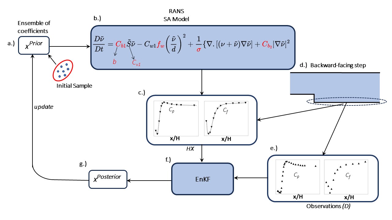
Figure 1: EnKF calibration loop, a.) An ensemble ($X$) of the SA coefficients - for the first iteration $X$ is sampled from a initial distribution determined by a parametric analysis in A . b.) The RANS solver and SA model calculate the flow variables based on the SA coefficients in $X$, the coefficients used in ensemble are highlighted in red, the coefficient $b$ is defined later. c.) The extracted quantities of interest (QOIs) from OpenFOAM at specified locations serve as the $HX$ for the EnKF. d.) The QOI in the current study are $C_{f}$ and $C_{p}$ along the bottom wall. e.) $D_{m\times N}$ matrix for the available data for QOI, $m$ is number of probe points $N$ is the ensemble size picked from the Gaussian distribution. g.) Updated $X^{p}$ based on the EnKF in f.

EnKF possesses desirable attributes such as the ability to accommodate noisy data, quantification of uncertainty, and enabling gradient-free optimization. Notably, the gradient-free optimization not only streamlines the EnKF’s implementation process but also endows it with heightened adaptability for integration with diverse computational fluid dynamics solvers, thereby reducing the necessity for intrusive modifications of their source code.
In addition, the $HX$ can be easily modified to use any QOI for which the calibration data is available. This customization process requires the (usually straightforward) extraction of the requisite QOI directly from the solution field.
Moreover, the EnKF’s proficiency in effectively managing noisy data aligns well with experimental data that has inherent measurement variabilities. This particular attribute underscores the EnKF’s suitability for assimilating real-world experimental observations into the calibration process, thereby enhancing its efficacy in bridging theoretical models with empirical data.

3.3 Calibration data (D)

We begin this section by noting that the data-driven calibration proposed in this research relied solely on experimental data. This is in contrast to similar studies which relied on DNS data for improving RANS models [30]. The requirement of only using experimental data presented challenges since the available data covered only a limited portion of the domain compared to DNS. This aligns with common data acquisition practices, as data is typically gathered predominantly along the walls, making it sparse, and it naturally contains some level of noise in the readings. Consequently, the calibration process proposed necessitated a robust handling of sparsity and noise inherent in the experimental data.
The experimental data for current study is from Driver and Seegmiller [33] and is retrieved the from NASA turbulence repository [33, 37]. The data consists of $C_{f}$ and $C_{p}$ measurements along the bottom wall of the BFS downstream of the step. The data was interpolated to 112 locations along the bottom of the wall, i.e. $m=112$. Notably, the magnitude of $C_{p}$ is approximately 3 orders of magnitude higher than the $C_{f}$. This difference in magnitude can cause the calibration to be weighted more towards $C_{p}$. Hence, the values of both $C_{p}$ and $C_{f}$ are separately scaled between $(0,1)$. Furthermore, a normally distributed noise $\epsilon\sim\mathcal{N}(0,\sigma_{D}=0.05)$, is added to the experimental data and $N=5$ data vectors are sampled to formulate our $D$ matrix. Figure 2 shows the mean value of observations.

Figure 2: Mean of the calibration data $D$, used for current study. The values of $C_{f}$ and $C_{p}$ are plotted along the bottom wall of BFS. The baseline data was obtained from the NASA turbulence repository [37] and a noise $\epsilon\sim\mathcal{N}(0,\sigma_{D}=0.05)$ is added to formulate the $D$ matrix.

3.4 Ensemble matrix (X)

To reiterate, the $X$ matrix for this study is formulated by coefficients of the SA model. A parametric analysis outlined in A was performed to select the SA coefficients for calibration, namely, $C_{b1},C_{w2},C_{w3},\sigma$ and $C_{v1}$ were selected. The parametric space for ensemble members is: $C_{w2}\in[0.75,1.75]$, $C_{w3}\in[1,2]$, $\sigma\in[0.3,2]$, and $C_{v1}\in[6,9]$.
In the original SA, $C_{b1}$ has a value of 0.1355 for the entire domain, however, after an initial study (B) it was found that implementing a varying $C_{b1}$ yields more flexibility in the model and may aid in improved calibration. Hence, the $C_{b1}$ is further parameterized in terms of non-dimensional field $r$ as follows:

$$C_{b1}=min\left(r*b,0.1355\right)+\alpha$$ (7)

where, $r\equiv\nu_{t}/Sk^{2}d^{2}$, 0.1355 is the original value of $C_{b1}$, $\alpha=10^{-6}$ is a scalar added to account for conditions where $r$ takes the value 0. The parameter $b\in[1.5,2.5]$ are also added to the ensemble matrix of the EnKF. To summarize, there are a total of five parameters that are calibrated using EnKF in this study.

3.5 Calibration metrics

The $X$ matrix is calibrated in an iterative manner as discussed in section 3.2. The performance of the calibration is monitored using the change in $X$ each iterations, specifically, as $\Delta X^{i}=mean(|X^{i}-X^{i-1}|)$ for $i^{it}$ iteration. The EnKF loop is run for 30 iterations. Figure 3 shows $\Delta X$ vs. iterations. The $\Delta X^{30}=0.003$ at the end of the EnKF deployment is considered acceptable for convergence. This is also evident from A, where such small changes in $X$ do not result in any variation of the QOI.

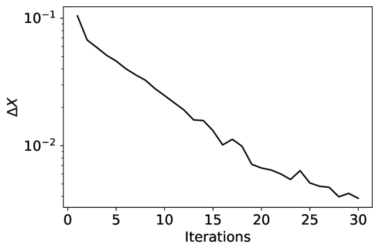
Figure 3: $\Delta X$ vs. iterations for the calibration loop.

The mean of the members of the posterior $X^{p}$ is obtained as: $b=1.38$, $\sigma=0.97$, $C_{w2}=0.78$, $C_{w3}=0.67$, and $C_{v1}=8.26$. The plots of $C_{b1}$ and $f_{w}$ using the calibrated coefficients are given in figure 4a and 4b. In figure 4b, the mapping (NN) of $f_{w}$ from the study of Bin et al. [30] is also compared to the current mapping. From here it can be concluded that the $f_{w}$ in Eq 3 provides enough flexibility to learn new mappings by changing $C_{w2}$ and $C_{w3}$. This further supports the hypothesis of Ray et al. [7], regarding the inadequacies in coefficients rather than model itself.

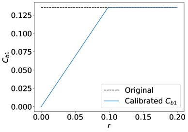
(a)

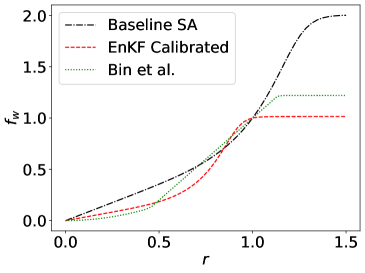
(b)

Figure 4: a. $C_{b1}$, b. $f_{w}$ vs. $r$ obtained from the calibrated coefficients. The original values are also plotted in corresponding plots. For additional comparison the $f_{w}$ obtained by Bin et al. [30] is also plotted.

4 Results

In this section the calibrated model is tested for various flows. The tested flows are classified in three categories: separated, attached and unbounded flows. The calibrated model is evaluated for improved performance on separating flows, while retaining the same good performance in attached and unbounded flows.

4.1 Separated flows

In this section, three separated flows are analyzed namely, BFS [33], 2D-bump [34], BFS2 (changed step height) [35, 30].

4.1.1 Flow over a BFS

In this section, the results for the flow over BFS are outlined. This flow was also used to calibrate the SA model using a relatively coarser mesh ($\approx 13000$ cells). The finer mesh ($\approx 28000$ cells) of test case also serves as a good indicator for the soft evaluation of the calibration across different meshes. Figure 5 compares the $C_{f}$ and $C_{p}$ plots from the calibrated SA model with that of the original SA; experimental data are also plotted for the purpose of comparison. It can be seen that the calibration significantly improves the results for the SA model, i.e., the results are closer to the experimental data used for calibration. Figure 5a shows the $C_{f}$ in recovery zone is more accurately predicted by the calibrated model. In addition there is significant improvement in the magnitude of the $C_{f}$ in separation bubble. Similar improvements are also observed in $C_{p}$ figure 5b. The reattachment length in the calibrated model is also closer to the experimental values as shown in figure 6.

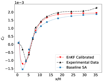
(a)

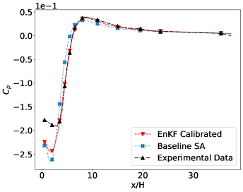
(b)

Figure 5: BFS: a.) $C_{f}$, b.) $C_{p}$ vs. $x/H$. The calibrated SA shows improvement in both recovery zone and separation bubble as compared to baseline model. The improvement in this case is defined as proximity to the experimental results.

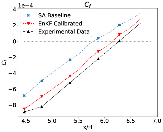
Figure 6: BFS: $C_{f}$ vs. $x/H$ showing the improved reattachment location ($C_{f}=0$) for the calibrated model.

Further analysis suggested that each coefficient of calibrated SA impacted improvement in results in a very specific manner. Notably, $C_{b1}$ and $f_{w}(C_{w2},C_{w3})$ influenced separation and recovery zone respectively. The effect is more evident in $C_{f}$, hence figure 7 shows only the results for $C_{f}$.
As shown in figure 7, if the baseline value of $C_{b1}=0.1355$ was used while using the calibrated values for rest of the coefficients the improvement is mainly observed in recovery zone, while the separation zone remains similar in magnitude to the baseline SA model. On the contrary, if baseline $f_{w}(C_{w2},C_{w3})$ is used in combination with the rest of calibrated coefficients the separation zone improves while recovery zone remains closer to the baseline SA. However, the best results are obtained by using all the calibrated coefficients. These results are consistent with the observation of Bin et al. [30] who used $f_{w}$ as NN to calibrate the SA model while keeping rest of the values same. They also observed an improved recovery zone with a slight reduction of accuracy in the separation zone.

(a)

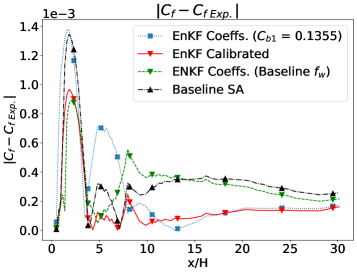
(b)

Figure 7: BFS: a.) $C_{f}$ vs. $x/H$ showing the impact of $C_{b1}$ and $f_{w}$ individually on the calibration results. If baseline $C_{b1}$ is used along with rest of the calibrated values (dotted blue), the results only show improvement in recovery zone, while remaining almost similar in separation bubble. On the other hand, if baseline $f_{w}(C_{w2},C_{w3})$ is used along with rest of calibrated coefficients (dashed green) the improvement is mainly observed in separation zone while the results in recovery zone remain close to the baseline SA. b.) Absolute error w.r.t the experimental data for each configuration vs. $X/H$.

From figure 7, it is evident that the $C_{b1}$ and $f_{w}$ have a domain-specific effect. In order to gain further understanding of how these coefficients vary through out the domain, we provide contour plots in Figure 8. The $C_{b1}$ takes particularly low values near the separation zone. It can also be observed that trend of $C_{b1}$ and $f_{w}$ is almost opposite to each other through out the domain. This opposite trend shows correlation between $C_{b1}$ (production) and $f_{w}$ (destruction). This can also be inferred that instead putting the onus of balancing region based production and destruction solely on the $f_{w}$ as in baseline model, the current formulation involves $C_{b1}(r)$ working with $f_{w}$ to balance these quantities.

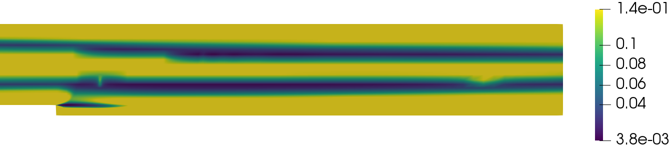
(a)

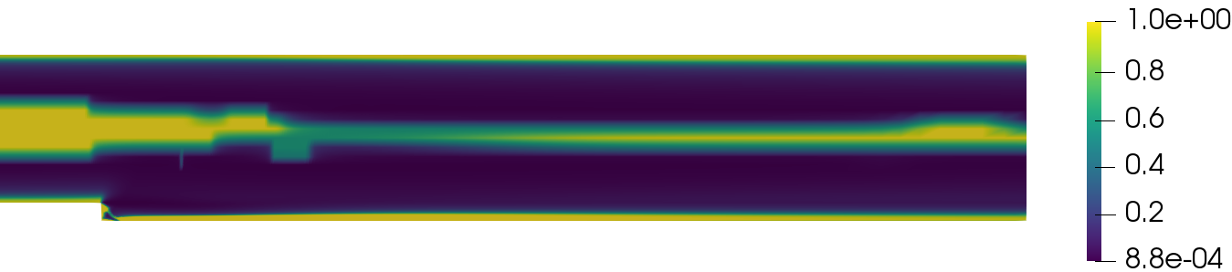
(b)

Figure 8: BFS: Variation of $C_{b1}$ and $f_{w}$ in the domain. Note that the original $C_{b1}$ possesses a constant value through out the domain.

4.1.2 2D-bump

The 2D-bump is a standard flow geometry in NASA turbulence repository [38]. The results for the 2D-bump are plotted in figure 9. The flow is attached to the bump upto $x/C=0.655$, after which separation is observed. In Figure 9a and b, until separation, the SA baseline and calibrated model are in good agreement with each other as well as experimental data [34, 38]. This agreement is encouraging as the calibration did not distort the performance of the data-enhanced model in attached flows. Furthermore, the calibrated model shows better recovery characteristics for $C_{f}$ for $x/C>1$. Overall, in figure 9b, the $C_{p}$ data from calibrated model shows a good agreement with experimental data. There are some deviations observed around $0.7<x/C<1$. However, it can be concluded that the calibrated model $C_{f}$ predictions are in better agreement with the experimental data as compared to the baseline case. On other hand, the $C_{p}$ predictions are closer to the baseline SA model than experimental data.

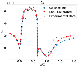
(a)

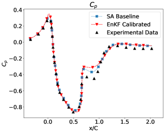
(b)

Figure 9: 2D-bump: a.) $C_{f}$, b.) $C_{p}$ vs. $x/C$, where $C$ is the chord length of the bump.

Similar to figure 7, a parametric analysis was also done for the 2D-bump case as shown in figure 10. The results shows similar trends to figure 7, which is encouraging for consistency and generalization of the calibrated model. As observed previously, the $C_{b1}$ affects the separation zone while $f_{w}$ affects the recovery zone. In Figure 10, by choosing the $C_{b1}=0.1355$ (original value) while keeping other values from calibration, results in faster recovery of $C_{f}$, implying the effect of calibrated coefficients ($f_{w}$) on recovery zone. On the contrary using a baseline $f_{w}$ with other coefficients being calibrated shows very slow recovery. Figure 11 shows the contour plots of $C_{b1}$ and $f_{w}$ for the 2D-bump. As with the BFS case (figure 8), the $C_{b1}$ and $f_{w}$ also follow an opposite trend to each other. The $C_{b1}$ takes lower values near the separation zone and increases to the the 0.1355 downstream of the bump.

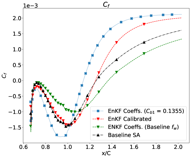
Figure 10: 2D-bump: $C_{f}$ vs. $x/C$, plotted after after the separation point $x/C>0.655$. Parametric analysis of calibrated coefficients by using baseline values in $C_{b1}$ and $f_{w}$ alternatively. The dotted blue line shows $C_{f}$ where, calibrated coefficients are paired with $C_{b1}$. The dashed green line shows the calibrated coefficients paired with baseline $f_{w}$. The red and black line show the results from calibrated and baseline models respectively.

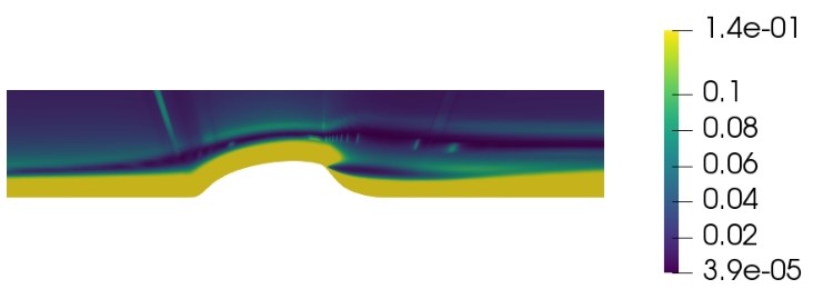
(a)

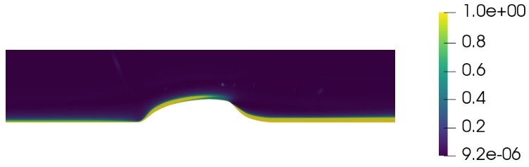
(b)

Figure 11: 2D-bump: Variation of $C_{b1}$ and $f_{w}$ in the domain.

4.1.3 Flow over backward-facing step (changed height, BFS2)

The calibrated model was further tested on a new backward-facing step case with a changed step height and $Re\approx 5600$ [30, 35]. The case is derived from the study of Bin et al. [30], who also used to test it for their DNS-calibrated SA model. The step height is 2m i.e., half of the domain height and $Re\approx 5600$. Figure 12 compares the agreement of $C_{f}$ from calibrated and baseline SA with that of direct numerical simulation(DNS) from Bin et al. [30]. In addition the results of the Bin et al. model are also presented for comparison. The results of figure 12 show better agreement of $C_{f}$ between our calibrated model and DNS when compared to the baseline SA model. In addition, the results show a better accuracy of current calibrated model in recirculating zone than the Bin et al. [30] calibrated model. The better results in the re-circulation zone are attributed to the calibration of $C_{b1}$ in addition to other coefficients whereas Bin et al. [30] only calibrate $f_{w}$ in their study.

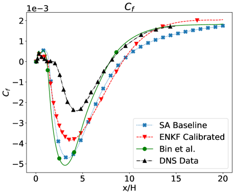
Figure 12: BFS2: $C_{f}$ vs. $x/H$ along bottom wall obtained from the calibrated coefficients is compared with DNS [30] and baseline SA. Additionally, the data from the calibrated SA model of Bin et al. [30] is also given.

For further establishing the role of $C_{b1}$ and $f_{w}$ on $C_{f}$, a similar analysis to figures 7 and 10 is performed on figure 13. The results are consistent with the previous results i.e., $C_{b1}$ affects the accuracy in the recirculating zone whereas the $f_{w}$ affect is predominant in the recovery zone.

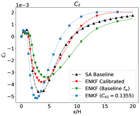
Figure 13: BFS2: Parametric analysis plotting $C_{f}$ vs. $x/H$ along bottom wall post step. The dashed green line displays the baseline $f_{w}$ combined with rest of EnKF calibrated coefficients, maintaining the initially observed improvement (figure 12) within the re-circulation zone but with a reduction in the recovery zone. Conversely, the dotted blue line depicts the baseline ($C_{b1}=0.1355$) along with rest of calibrated coefficients, sustaining the improvement in the recovery zone but a decrease in the re-circulation zone.

4.2 Unbounded or attached flow

We have established that the EnKF-based calibration improves the SA model’s performance in separated flows. However, the change in model parameters may distort the good performance of the model in unbounded or attached flows. In this section the calibrated model is compared with the original SA model to measure any deviation.

4.2.1 NACA0012

The model is first tested for an unbounded flow over a NACA0012 airfoil at the angles of attack $0^{\circ}$ and $10^{\circ}$ in figure 14 and 15, respectively [39, 40]. The calibrated model shows an excellent agreement with the original SA model – and we conclude that the performance of the original model is preserved in the calibrated variant.

(a)

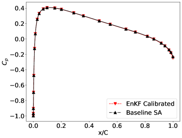
(b)

Figure 14: NACA0012 airfoil at angle of attack $0^{\circ}$: a. $C_{f}$, b. $C_{p}$ vs. $x/C$. The calibrated model shows good agreement with the original model. Hence, no distortion in good behaviour of the SA model is observed for unbounded flows over an airfoil.

(a)

(b)

Figure 15: NACA0012 airfoil at angle of attack $10^{\circ}$: a. $C_{f}$, b. $C_{p}$ vs. $x/C$.

4.2.2 Flat plate boundary layer

The improved model was further tested on a zero pressure gradient flat plate boundary layer flow to determine any distortion from the standard SA model in attached flows. Figure 16a and b show the $C_{f}$ and $C_{p}$ vs. $Re_{x}$ plots for the calibrated and baseline model. From here, it can be inferred that the calibrated SA model does not distort the behaviour of the baseline model in attached or unbounded flows.

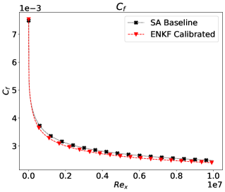
(a)

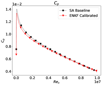
(b)

Figure 16: Zero pressure gradient boundary layer: a. $C_{f}$, b. $C_{p}$ vs. $Re_{x}$ for flow over a flat plate showing no distortion in the behaviour of calibrated model for attached flows.

5 Conclusions

An EnKF-based calibration methodology has been introduced for improving RANS closure models with limited and noisy experimental data. The focus was on the SA model’s performance in separated flows. Through this methodology, the SA coefficients were effectively adjusted, potentially minimizing the need for black-box ML-models like NNs which may fail to generalize. The calibrated SA model exhibited improved accuracy in predicting important flow quantities, specifically $C_{p}$ and $C_{f}$, in scenarios involving separated flows. Notably, this improvement was achieved without compromising the SA model’s accuracy in predicting behavior in attached and unbounded flows, aligning well with the progressive nature of SA enhancements.
The findings further corroborate the hypothesis put forth by Ray et al. [7], demonstrating that a substantial portion of closure model errors can be rectified by coefficient adjustments. The calibration process utilized only one geometry, namely BFS, at a single $Re$. Owing to the generalization provided by SA model, this approach successfully extended the calibrated model’s applicability to extrapolated cases and scenarios beyond its training range. In contrast, such stringent training criteria could lead to overfitting and extrapolation in the context of deep neural network applications.
The adaptability of the original $f_{w}$ function (equation 3) was also evident in this study, as the calibrated $C_{w2}$ and $C_{w3}$ coefficients displayed trends similar to those captured by a trained NN (as seen in figure 4b). Another notable advancement involved the treatment of $C_{b1}$ as a function of $r$ instead of a fixed scalar value found in the baseline SA model. This increased flexibility in representing $C_{b1}$ notably enhanced the calibrated model’s predictive capabilities within re-circulation zones. The interplay between $C_{b1}$ and $f_{w}$ was also evident, where the former significantly impacted re-circulation zone prediction while the latter influenced recovery zone predictions.
The stochastic nature of the EnKF necessitated a thoughtful selection of coefficient sampling ranges, a process guided by a parametric analysis (A). This range determination intricately hinged on an understanding of the relationships between production, destruction, and diffusion terms. Nonetheless, the possibility of relaxing this selection criterion through calibrations with multiple flow conditions remains a viable avenue for future exploration within the study’s scope.

Appendix A Parametric analysis for SA model

In this section, a parametric analysis by varying the SA coefficients is performed. The underlying objective is to enhance our comprehension of how alterations in coefficient values influence the QOIs, such as $C_{f}$ and $C_{p}$, in the context of separation phenomena. This analysis significantly contributes to the selection of coefficients, along with their respective bounding values, that collectively constitute the formulation of the matrix $X$. Figures 17 and 18 outline the results of the analysis.

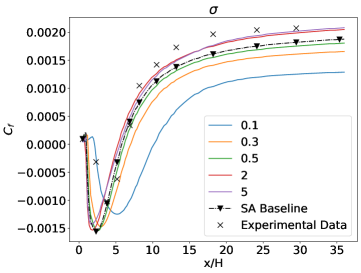
(a)

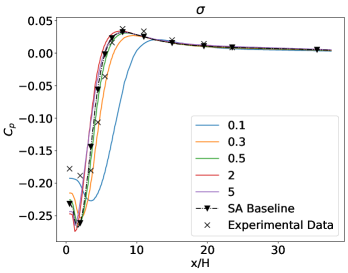
(b)

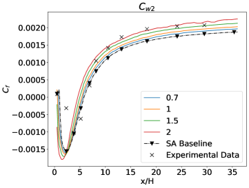
(c)

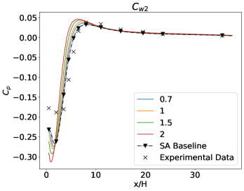
(d)

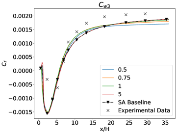
(e)

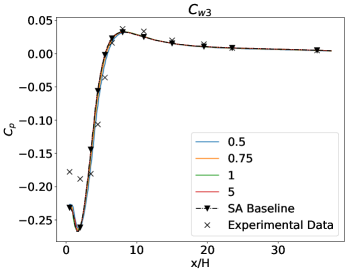
(f)

Figure 17: Parametric analysis for $C_{f}$ and $C_{p}$ along the bottom wall of the BFS by varying $\sigma$ (a,b), $C_{w2}$ (c,d), $C_{w3}$ (e,f). For reference the solutions with original SA coefficients along with experimental data [37] is also given. The title of each subplot is the SA coefficient that was varied for analysis.

Figure 17a and b present the variations in $C_{f}$ and $C_{p}$ with different $\sigma$ values. The parameter $\sigma$ influence the diffusivity within the SA equation. Notably, observable changes in both $C_{f}$ and $C_{p}$ occur in response to alterations in $\sigma$ values. Consequently, the choice of $\sigma$ assumes importance as a target for optimization in EnKF.
The range $\sigma\in[0.3,2]$ yields results in the vicinity of experimental data. Values below 0.3, such as $\sigma=0.1$, deviate substantially from the experimental data, while $\sigma=5$ displays minimal variance compared to the results at 2. This lack of variation at $\sigma>2$ does not incentivize an expansion of the sample space. Hence, the interval [0.3, 2] emerges as the preferred range for $\sigma$ sampling in the $X$ matrix.
Figure 17 c-f, show the variation of $C_{f}$ and $C_{p}$ w.r.t $C_{w2}$ and $C_{w3}$. These two coefficients collectively contribute to the parameter $f_{w}$ (as depicted in eq. 3). This parameter plays a pivotal role in governing the destruction of eddy viscosity.
The selection of $C_{w2}$ and $C_{w3}$ for $X$ matrix stems from their direct influence on $f_{w}$. Notably, $f_{w}$ affects the SA’s predictions for wall bounded non equilibrium flows [1, 15, 30]. Particularly, Bin et al. [30], outline the impact of $f_{w}$ on the behavior of skin friction coefficient ($C_{f}$) in recovery zone.
The interval [0.75, 1.75], is chosen for sampling $C_{w2}$. This range is chosen because the for different regions the values of $C_{f}$ and $C_{p}$ improve based on the values $C_{w2}$. In addition, $C_{p}$ and $C_{f}$, follow mutually opposite trend for increase or decrease of the $C_{w2}$. It was observed that for the values in range [0.75, 1.75], the QOI takes the values that are more closer to the experimental data for entire region.
Similarly, the interval [1,2] is decided for the $C_{w3}$. A slight improvement in recovery zone for $C_{f}$ is observed at $C_{w3}=1$, which is also selected as the lower bound of the sample space owing to deteriorated accuracy at $C_{w3}<1$ at $x/H>25$, i.e., 0.75 and 0.5. For upper limit the value of 2 (SA baseline) is selected owing to non-observable difference between the results at the values of 2 and 5. Additionally the upper bound is motivated by the original value of $C_{w3}=2$ is SA model.

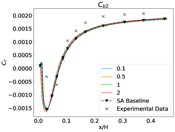
(a)

(b)

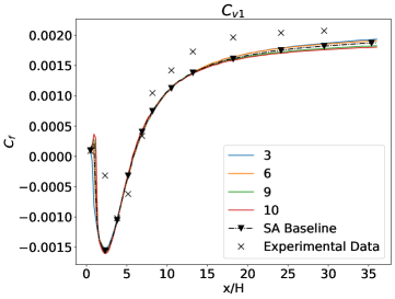
(c)

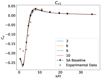
(d)

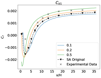
(e)

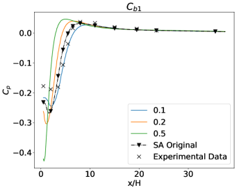
(f)

Figure 18: Parametric analysis by varying $C_{b2}$ (a,b), $C_{v1}$ (c,d), $C_{b1}$ (e,f). For reference the solutions with original SA coefficients along with experimental data [37] is also given.

Figures 18a and b depict the results of a parametric analysis involving the variation of $C_{b2}$. The observed variations in both $C_{f}$ and $C_{p}$ due to changes in $C_{b2}$ are not substantial. Consequently, $C_{b2}$ is not deemed influential enough to warrant selection for the optimization process.
Similarly, Figures 18c and d illustrate the impact of variations in $C_{v1}$ on $C_{f}$ and $C_{p}$. Although alterations in $C_{v1}$ have a limited effect on both coefficients, discernible variations emerge in the far downstream region for $C_{f}$ and the recovery region for $C_{p}$. As a result of these observations, $C_{v1}$ is chosen for the optimization process.
For the optimization of $C_{v1}$, the selected range of variation is [6, 9]. This range is informed by the improved performance of $C_{f}$ at higher values of $C_{v1}$. Hence, the sample space is slightly biased towards values higher than baseline $C_{v1}=7.1$.
Figure 18 e and f shows significant influence of varying $C_{b1}$ on $C_{f}$ and $C_{p}$. Therefore, $C_{b1}$ is also selected for the optimization. However, for the purpose of this study the $C_{b1}$ is further parameterized as a function of $r$, where $r\equiv\nu_{t}/Sk^{2}d^{2}$.

Appendix B Parametrization of $C_{b1}$

From Figure 18e, it becomes evident that when $C_{b1}=0.1$, the behavior of skin friction coefficient ($C_{f}$) in the re-circulation region aligns more closely with the experimental data. Conversely, with $C_{b1}=0.2$, better performance is observed in the recovery zone. While this region-specific impact is observable for other coefficients as well, it is particularly pronounced in the case of $C_{b1}$. Hence, $C_{b1}$ is paramterized further. This extension allows $C_{b1}$ to adopt different values contingent on the flow and domain characteristics. Drawing inspiration from eq. 3, which parameterizes $f_{w}$ in terms of $r$, it was deemed appropriate to express $C_{b1}$ as a function of $r$ as well. Though rest of the coefficients can also be parameterized further, but for in the scope of current study only $C_{b1}$ is parameterized.
For the sake of simplicity, current study parameterized the $C_{b}1$ as a linear function of $r$ as shown in eq. 8. The upper bound $C_{b1}$ is limited to its default value of 0.1355 using a $min$ function. This has upper bound has effect of plateauing on the $C_{b1}$ function which is similar to the $f_{w}$. This will hep to ensure the consistency between production and destruction term of the SA model, along with preserving the behaviour of the model in equilibrium flows. The $\alpha$ is a small scalar whose value is set to $10^{-6}$, which takes effect only if the value of $r$ goes to zero. The simplistic nature of the eq. 8 and the improvements due to it are encouraging. However, the equation used here is not claimed to be optimum for the paramterization and mildly violates the soft constraint proposed by Spalart et al. [15] for the data-driven studies, i.e. not using $min$ or $max$ functions. Hence, a more focused study can be conducted to explore equations that are more consistent for SA model. Another approach could be replace the eq. 8 by a NN.

$$C_{b1}=min\left(r*b,0.1355\right)+\alpha$$ (8)

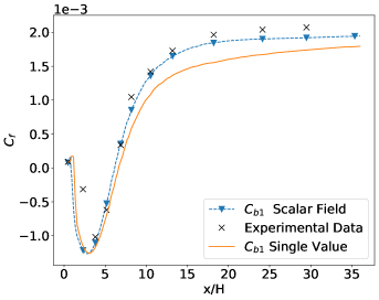
(a)

(b)

Figure 19: Comparison of EnKF calibration using $C_{b1}$ as a function of $r$ with $C_{b1}$ as constant scalar within the BFS domain. a.) $C_{f}$ and b.) $C_{p}$ along the bottom wall for both calibrations.

Figure 19 compares the EnKF calibration for both scenarios i.e. where the $C_{b1}$ is: i. Scalar field varying w.r.t $r$ and ii. Scalar field with a constant value through out the domain. Notably, rest of the coefficient in ensemble are same. Using $C_{b1}$ as a function of $r$ yield results closer to the experimental values and hence was preferred approach for current study.

References

- [1] P. Spalart, S. Allmaras, A one-equation turbulence model for aerodynamic flows, in: 30th aerospace sciences meeting and exhibit, 1992, p. 439.
- [2] T. Craft, B. Launder, K. Suga, Development and application of a cubic eddy-viscosity model of turbulence, International Journal of Heat and Fluid Flow 17 (2) (1996) 108–115.
- [3] R. H. Bush, T. S. Chyczewski, K. Duraisamy, B. Eisfeld, C. L. Rumsey, B. R. Smith, Recommendations for future efforts in rans modeling and simulation, in: AIAA scitech 2019 forum, 2019, p. 0317.
- [4] K. Duraisamy, G. Iaccarino, H. Xiao, Turbulence modeling in the age of data, Annual review of fluid mechanics 51 (2019) 357–377.
- [5] B. D. Tracey, K. Duraisamy, J. J. Alonso, A machine learning strategy to assist turbulence model development, in: 53rd AIAA aerospace sciences meeting, 2015, p. 1287.
- [6] Y. Yin, Z. Shen, Y. Zhang, H. Chen, S. Fu, An iterative data-driven turbulence modeling framework based on reynolds stress representation, Theoretical and Applied Mechanics Letters 12 (5) (2022) 100381.
- [7] J. Ray, L. Dechant, S. Lefantzi, J. Ling, S. Arunajatesan, Robust bayesian calibration of ak- model for compressible jet-in-crossflow simulations, AIAA Journal 56 (12) (2018) 4893–4909.
- [8] L. Zhu, W. Zhang, J. Kou, Y. Liu, Machine learning methods for turbulence modeling in subsonic flows around airfoils, Physics of Fluids 31 (1) (2019).
- [9] L. Zhu, W. Zhang, X. Sun, Y. Liu, X. Yuan, Turbulence closure for high reynolds number airfoil flows by deep neural networks, Aerospace Science and Technology 110 (2021) 106452.
- [10] X. Sun, W. Cao, Y. Liu, L. Zhu, W. Zhang, High reynolds number airfoil turbulence modeling method based on machine learning technique, Computers & Fluids 236 (2022) 105298.
- [11] R. Maulik, H. Sharma, S. Patel, B. Lusch, E. Jennings, A turbulent eddy-viscosity surrogate modeling framework for reynolds-averaged navier-stokes simulations, Computers & Fluids 227 (2021) 104777.
- [12] Y. Liu, W. Cao, W. Zhang, Z. Xia, Analysis on numerical stability and convergence of reynolds averaged navier–stokes simulations from the perspective of coupling modes, Physics of Fluids 34 (1) (2022).
- [13] J. Ling, A. Kurzawski, J. Templeton, Reynolds averaged turbulence modelling using deep neural networks with embedded invariance, Journal of Fluid Mechanics 807 (2016) 155–166.
- [14] S. B. Pope, A more general effective-viscosity hypothesis, Journal of Fluid Mechanics 72 (2) (1975) 331–340.
- [15] P. Spalart, An old-fashioned framework for machine learning in turbulence modeling, arXiv preprint arXiv:2308.00837 (2023).
- [16] J.-X. Wang, J.-L. Wu, H. Xiao, Physics-informed machine learning approach for reconstructing reynolds stress modeling discrepancies based on dns data, Physical Review Fluids 2 (3) (2017) 034603.
- [17] J.-L. Wu, H. Xiao, E. Paterson, Physics-informed machine learning approach for augmenting turbulence models: A comprehensive framework, Physical Review Fluids 3 (7) (2018) 074602.
- [18] J. Wu, H. Xiao, R. Sun, Q. Wang, Reynolds-averaged navier–stokes equations with explicit data-driven reynolds stress closure can be ill-conditioned, Journal of Fluid Mechanics 869 (2019) 553–586.
- [19] R. McConkey, E. Yee, F.-S. Lien, Deep structured neural networks for turbulence closure modeling, Physics of Fluids 34 (3) (2022).
- [20] M. Shirzadi, P. A. Mirzaei, Y. Tominaga, Rans model calibration using stochastic optimization for accuracy improvement of urban airflow cfd modeling, Journal of Building Engineering 32 (2020) 101756.
- [21] C. Grabe, F. Jäckel, P. Khurana, R. P. Dwight, Data-driven augmentation of a rans turbulence model for transonic flow prediction, International Journal of Numerical Methods for Heat & Fluid Flow 33 (4) (2023) 1544–1561.
- [22] J. Ray, S. Lefantzi, S. Arunajatesan, L. Dechant, Bayesian parameter estimation of ak- model for accurate jet-in-crossflow simulations, AIAA Journal 54 (8) (2016) 2432–2448.
- [23] V. Yakhot, S. Orszag, S. Thangam, T. Gatski, C. Speziale, Development of turbulence models for shear flows by a double expansion technique, Physics of Fluids A: Fluid Dynamics 4 (7) (1992) 1510–1520.
- [24] K. Duraisamy, Z. J. Zhang, A. P. Singh, New approaches in turbulence and transition modeling using data-driven techniques, in: 53rd AIAA Aerospace sciences meeting, 2015, p. 1284.
- [25] A. P. Singh, K. Duraisamy, Z. J. Zhang, Augmentation of turbulence models using field inversion and machine learning, in: 55th AIAA Aerospace Sciences Meeting, 2017, p. 0993.
- [26] A. P. Singh, K. Duraisamy, Using field inversion to quantify functional errors in turbulence closures, Physics of Fluids 28 (4) (2016).
- [27] M. Yang, Z. Xiao, Improving the k–––ar transition model by the field inversion and machine learning framework, Physics of Fluids 32 (6) (2020).
- [28] E. J. Parish, K. Duraisamy, A paradigm for data-driven predictive modeling using field inversion and machine learning, Journal of computational physics 305 (2016) 758–774.
- [29] C. Yan, H. Li, Y. Zhang, H. Chen, Data-driven turbulence modeling in separated flows considering physical mechanism analysis, International Journal of Heat and Fluid Flow 96 (2022) 109004.
- [30] Y. Bin, G. Huang, X. I. Yang, Data-enabled recalibration of the spalart–allmaras model, AIAA Journal (2023) 1–12.
- [31] X.-L. Zhang, H. Xiao, X. Luo, G. He, Ensemble kalman method for learning turbulence models from indirect observation data, Journal of Fluid Mechanics 949 (2022) A26.
- [32] G. Evensen, et al., Data assimilation: the ensemble Kalman filter, Vol. 2, Springer, 2009.
- [33] D. M. Driver, H. L. Seegmiller, Features of a reattaching turbulent shear layer in divergent channelflow, AIAA journal 23 (2) (1985) 163–171.
- [34] A. Seifert, L. G. Pack, Active flow separation control on wall-mounted hump at high reynolds numbers, AIAA journal 40 (7) (2002) 1363–1372.
- [35] M. Barri, G. K. El Khoury, H. I. Andersson, B. Pettersen, Dns of backward-facing step flow with fully turbulent inflow, International Journal for Numerical Methods in Fluids 64 (7) (2010) 777–792.
- [36] J. Mandel, Efficient implementation of the ensemble Kalman filter, Center for Computational Mathematics, University of Colorado at Denver, 2006.
- [37] Turbulence Modeling Resource: 2D backward facing step., https://turbmodels.larc.nasa.gov/backstep_val_sa.html, accessed: 2023–06-07.
- [38] Turbulence Modeling Resource: 2D wall mounted hump., https://turbmodels.larc.nasa.gov/nasahump_val.html, accessed: 2023–06-07.
- [39] T. F. Brooks, M. A. Marcolini, D. S. Pope, Airfoil trailing-edge flow measurements, AIAA journal 24 (8) (1986) 1245–1251.
- [40] A. Di Mascio, R. Broglia, R. Muscari, Prediction of hydrodynamic coefficients of ship hulls by high-order godunov-type methods, Journal of marine science and technology 14 (2009) 19–29.