SIGW short = SIGW , long = scalar induced gravitational wave , short-plural = s \DeclareAcronymSGWB short = SGWB , long = stochastic gravitational wave background , short-plural = \DeclareAcronymPTA short = PTA , long = pulsar timing array , short-plural = \DeclareAcronymGWs short = GWs, long = gravitational waves
Scalar Induced Gravitational Waves from Finslerian Inflation and Pulsar Timing Arrays Observations
Abstract
The recent data from NANOGrav provide strong evidence of the existence of the \acpSGWB. We investigate \acpSIGW from Finslerian inflation as a potential source of stochastic gravitational wave background. Small-scale (1 Mpc) statistically anisotropic primordial scalar perturbations can be generated in Finslerian inflation. The second order \acpSIGW from Finslerian inflation are also anisotropic on small scales. After spatially averaging the small-scale anisotropic \acpSIGW, we obtain the large-scale isotropic \acpSGWB. We find that the parameters of small-scale anisotropic primordial power spectrum generated by Finslerian inflation affect the \acpPTA observations of large-scale isotropic gravitational wave background.
keywords:
pulsar timing arrays – inflation – Finsler spacetime – scalar induced gravitational waves1 Introduction
Recently, the stochastic gravitational wave background (SGWB) in the nHz frequency range has been strongly supported by the collective evidence from various \acPTA observations, such as NANOGrav (Agazie et al. (2023a, b); Afzal et al. (2023)), EPTA (Antoniadis et al. (2023a, b, c, d, e); Smarra et al. (2023)), PPTA (Reardon et al. (2023a, b); Zic et al. (2023)), and CPTA (Xu et al. (2023)). The origin of \acSGWB remains unclear on account of the complexity of the sources. For cosmological origin, several mechanisms have been proposed to explain the \acPTA observations, including cosmic strings and domain walls (Ellis et al. (2023); Kitajima et al. (2023); Bai et al. (2023)), cosmological phase transition (Fujikura et al. (2023); Bringmann et al. (2023)), primordial black hole (PBH) merger (Depta et al. (2023)), self-interacting dark matter (SIDM) (Han et al. (2023)), \acSIGW (Balaji et al. (2023); Cai et al. (2023); Zhu et al. (2023); Wang et al. (2023)) and so on.
In this paper, we consider the second order \acpSIGW as a potential origin for the \acpSGWB. Since the second order \acpSIGW are generated by the primordial scalar perturbations for specific inflation model, the parameters of that model can be constrained by the current \acPTA observations. Here, we investigate the second order GWs generated by small-scale (1 Mpc) statistically anisotropic primordial scalar perturbations in Finslerian inflation. Finslerian inflation is based on the modified gravity in Finsler geometry which has been studied for many years (Chang & Li (2008, 2009); Pfeifer & Wohlfarth (2011, 2012); Li & Chang (2014); Russell (2015)). The anisotropic primordial power spectra in Finslerian inflation were studied in Ref. (Li et al. (2015); Chang et al. (2018)), it can be used to explain both parity asymmetry and power deficit seen in CMB temperature anisotropies (Chang et al. (2018)). Furthermore, the anisotropic primordial power spectra can also be realized by other inflation scenarios (Ackerman et al. (2007); Soda (2012); Maleknejad et al. (2013); Dimastrogiovanni et al. (2010); Chen & Ota (2022)).
In Finslerian inflation, the energy density spectra of second order \acpSIGW are also anisotropic on small scale. Since the small-scale anisotropic of SGWBs can not be observed by current PTA observations (detalis can be found in Ref. (Bartolo et al. (2020); Li et al. (2023))), we derive the isotropic gravitational wave background on large scales in terms of spatially averaging the anisotropic gravitational wave background at small scales. We find that the spatial averaging does not eliminate the influence of the anisotropic parameters in Finslerian inflation. Namely, the potential small-scale anisotropic primordial power spectra can be constrained by the \acpPTA observations of large-scale isotropic SGWBs.
The remainder of this paper is organized as follows: Section 2 introduces the primordial scalar perturbation in Finsler spacetime. In Section 3, we present the formula for \acpSIGW. In Section 4, we calculate the energy density of \acpSIGW within the context of Finslerian inflation. Then, we constrain the parameter space of Finslerian inflation in terms of PTA observations. We summarize our results in Section 5.
2 Primordial Perturbation From Finsler Spacetime
Finsler geometry is a natural generalization of Riemann geometry in absence of quadratic restriction (Bao et al. (2000)). The Finslerian metric is defined as
| (1) |
where is called Finsler structure which satisfies
| (2) |
Following Ref. (Li et al. (2015)), the background spacetime in Finslerian inflation can be written as
| (3) |
where denotes the Finsler structure of Randers space (Randers (1941))
| (4) |
The first term is Riemannian metric and the second term is a one form. takes the form of and is the parameter of anisotropy on small scales.
The equation of motion for the primordial scalar perturbation in Finslerian inflation can be written as (Li et al. (2015))
| (5) |
where and is the Finslerian metric with respect to Finsler structure in Eq. (3) and Eq. (4). For simplicity, the direction of in Eq. (4) is taken to be parallel to the wave vector in the momentum space. Then Eq. (5) becomes
| (6) |
where is the effective wavenumber
| (7) |
where . The primordial power spectrum can be derived as (Li et al. (2015); Mukhanov (2005))
| (8) |
where is the primordial power spectrum of the isotropic spacetime. represents the anisotropy in Finslerian inflation.
3 Second Order Scalar induced GWs
In this section, we briefly review the calculations of second order \acpSIGW which have been studied for many years (Domenech (2021); Kohri & Terada (2018); Zhou et al. (2022); Zhang et al. (2022)). For simplicity, the background spacetime is assumed to be Friedmann-Robertson-Walker (FRW) spacetime after inflation
| (9) |
where the superscript means this is a background quantity. The is the conformal time. In the Newtonian gauge, the perturbed metric is
| (10) |
where the superscript and represent first order and second order perturbation, respectively. The and are the scalar perturbations, which are equal in the Newtonian gauge. is the tensor perturbation.
The two-point correlation function of is defined as , where is the primordial power spectrum. Considering the second order perturbations of Einstein’s equation , we obtain the equation of motion of the second order \acpSIGW in momentum space
| (11) | ||||
where and . is polarization tensor which satisfies . is the conformal Hubble parameter. The source term is given by
| (12) | ||||
The first order scalar perturbation in Eq. (12) can be written as
| (13) |
where
| (14) |
is the transfer function. Substituting Eq. (13) into Eq. (12), we obtain
| (15) |
where takes the form of
| (16) | ||||
We have set , and . Using the Green’s function method to solve the equation (11), we obtain
| (17) |
where the kernel function is
| (18) |
Then, the power spectra of second order \acpSIGW can be evaluated in terms of the following equation
| (19) | ||||
4 Constraining Finslerian Inflation with Pulsar Timing Arrays Observations
In this section, we investigate the second order \acpSIGW from Finslerian inflation. In order to obtain the energy density spectrum of second order \acpSIGW in Finslerian inflation, we substitute Eq. (8) into Eq. (19)
| (20) | ||||
where and is the azimuth of . For isotropic primordial power spectra, the integral , then Eq. (20) reduces to Eq. (19). After taking the spatial average, we obtain the isotropic energy density fraction spectrum
| (21) | ||||
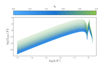
where and are the azimuth and elevation of in equation (20), respectively. Since the small-scale anisotropy can not be detected by current PTA observations, we integrate the space angle to obtain the isotropic energy density spectrum. Here, we consider a monochromatic primordial power spectrum, namely, . The corresponding energy density spectra for different is given in Fig. 1.
In order to constrain the parameter space of Finslerian inflation in terms of PTA observations, we need to convert the energy density into the energy density in present universe (Espinosa et al. (2018))
| (22) |
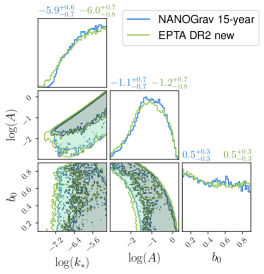
where is the radiation fraction today. Then, we use Ceffyl (Lamb et al. (2023)) package embed in PTArcade (Mitridate et al. (2023)) to analyze the data from the first 14 frequency bins of NANOGrav 15-year and the first 9 frequency bins in EPTA DR2 new. The priors of , and set as uniform distributions over the intervals , and , respectively. The posteriors distributions are shown in Fig. 2.
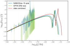
We now discuss the results of Bayesian analysis. In Fig. 2, we find an obvious band structure in the two-dimensional posterior distribution plot for and . It indicates the degeneracy between these two parameters. For second order \acpSIGW, altering the parameter results in a horizontal shift of energy density spectra on the - plot, while changing the parameter leads to a vertical shift. Consequently, these two parameters are degenerate with respect to the PTA observations. As shown in Fig. 2, NANOGrav and EPTA constrain to be near and respectively, while the constraints on are relatively weaker for both. For the parameters , which characterize small-scale anisotropies, the NANOGrav 15-year and EPTA data provide nearly identical marginal posterior probabilities for different values of . In Fig. 3, we directly combined the first 9 frequency bins from EPTA with the 14 frequency bins from NANOGrav to obtain the combined dataset. Subsequently, we processed the data following the same methodology previously applied to both datasets. The posterior probability distribution results are presented in Fig. 3. The combined posterior probability distribution favors a relatively smaller value of . As shown in Fig. 4, we plot the energy density spectra of second order \acpSIGW with the median values of the parameters , and .

5 CONCLUSION
We investigated second order \acpSIGW from Finslerian inflation as a potential origin of \acSGWB. Through Bayesian analysis of EPTA, NANOGrav 15-year, and combined data, we found that these datasets can constrain parameter but provide relatively weaker constraints on anisotropic parameters . These datasets may indicate an anisotropic primordial power spectrum on small scales. Future observations might impose more stringent constraints on anisotropies at small scales. As we mentioned, the anisotropic primordial power spectra can also be realized by other inflation scenarios, related studies might be presented in future works.
Acknowledgement
This work has been funded by the National Nature Science Foundation of China under grant No. 12075249, 11690022 and 12275276. And the Key Research Program of the Chinese Academy of Sciences under Grant No. XDPB15.
Data availability
References
- Ackerman et al. (2007) Ackerman L., Carroll S. M., Wise M. B., 2007, Phys. Rev. D, 75, 083502
- Afzal et al. (2023) Afzal A., et al., 2023, Astrophys. J. Lett., 951, L11
- Agazie et al. (2023a) Agazie G., et al., 2023a, Astrophys. J. Lett., 951, L8
- Agazie et al. (2023b) Agazie G., et al., 2023b, Astrophys. J. Lett., 951, L9
- Antoniadis et al. (2023b) Antoniadis J., et al., 2023b, The second data release from the European Pulsar Timing Array II. Customised pulsar noise models for spatially correlated gravitational waves (arXiv:2306.16225)
- Antoniadis et al. (2023c) Antoniadis J., et al., 2023c, The second data release from the European Pulsar Timing Array III. Search for gravitational wave signals (arXiv:2306.16214)
- Antoniadis et al. (2023d) Antoniadis J., et al., 2023d, The second data release from the European Pulsar Timing Array IV. Search for continuous gravitational wave signals (arXiv:2306.16226)
- Antoniadis et al. (2023e) Antoniadis J., et al., 2023e, The second data release from the European Pulsar Timing Array: V. Implications for massive black holes, dark matter and the early Universe (arXiv:2306.16227)
- Antoniadis et al. (2023a) Antoniadis J., et al., 2023a, ] 10.1051/0004-6361/202346841
- Bai et al. (2023) Bai Y., Chen T.-K., Korwar M., 2023
- Balaji et al. (2023) Balaji S., Domènech G., Franciolini G., 2023
- Bao et al. (2000) Bao D., Chern S.-S., Shen Z., 2000, An introduction to Riemann-Finsler geometry. Vol. 200, Springer Science & Business Media
- Bartolo et al. (2020) Bartolo N., et al., 2020, Journal of Cosmology and Astroparticle Physics, 2020, 028
- Bringmann et al. (2023) Bringmann T., Depta P. F., Konstandin T., Schmidt-Hoberg K., Tasillo C., 2023
- Cai et al. (2023) Cai Y.-F., He X.-C., Ma X., Yan S.-F., Yuan G.-W., 2023
- Chang & Li (2008) Chang Z., Li X., 2008, Phys. Lett. B, 668, 453
- Chang & Li (2009) Chang Z., Li X., 2009, Phys. Lett. B, 676, 173
- Chang et al. (2018) Chang Z., Rath P. K., Sang Y., Zhao D., Zhou Y., 2018, Mon. Not. Roy. Astron. Soc., 479, 1327
- Chen & Ota (2022) Chen C., Ota A., 2022, Physical Review D, 106
- Depta et al. (2023) Depta P. F., Schmidt-Hoberg K., Schwaller P., Tasillo C., 2023
- Dimastrogiovanni et al. (2010) Dimastrogiovanni E., Bartolo N., Matarrese S., Riotto A., 2010, Advances in Astronomy, 2010, 1
- Domenech (2021) Domenech G., 2021, Universe, 7, 398
- Ellis et al. (2023) Ellis J., Lewicki M., Lin C., Vaskonen V., 2023
- Espinosa et al. (2018) Espinosa J., Racco D., Riotto A., 2018, Physical Review Letters, 120
- Fujikura et al. (2023) Fujikura K., Girmohanta S., Nakai Y., Suzuki M., 2023
- Han et al. (2023) Han C., Xie K.-P., Yang J. M., Zhang M., 2023
- Kitajima et al. (2023) Kitajima N., Lee J., Murai K., Takahashi F., Yin W., 2023
- Kohri & Terada (2018) Kohri K., Terada T., 2018, Physical Review D, 97
- Lamb et al. (2023) Lamb W. G., Taylor S. R., van Haasteren R., 2023
- Li & Chang (2014) Li X., Chang Z., 2014, Physical Review D, 90
- Li et al. (2015) Li X., Wang S., Chang Z., 2015, Eur. Phys. J. C, 75, 260
- Li et al. (2023) Li J.-P., Wang S., Zhao Z.-C., Kohri K., 2023, Primordial Non-Gaussianity and Anisotropies in Gravitational Waves induced by Scalar Perturbations (arXiv:2305.19950)
- Maleknejad et al. (2013) Maleknejad A., Sheikh-Jabbari M., Soda J., 2013, Physics Reports, 528, 161
- Mitridate et al. (2023) Mitridate A., Wright D., von Eckardstein R., Schr"oder T., Nay J., Olum K., Schmitz K., Trickle T., 2023
- Mukhanov (2005) Mukhanov V. F., 2005, Physical foundations of cosmology. Cambridge university press
- Pfeifer & Wohlfarth (2011) Pfeifer C., Wohlfarth M. N. R., 2011, Physical Review D, 84
- Pfeifer & Wohlfarth (2012) Pfeifer C., Wohlfarth M. N. R., 2012, Physical Review D, 85
- Randers (1941) Randers G., 1941, Phys. Rev., 59, 195
- Reardon et al. (2023a) Reardon D. J., et al., 2023a, The Astrophysical Journal Letters, 951, L6
- Reardon et al. (2023b) Reardon D. J., et al., 2023b, The Astrophysical Journal Letters, 951, L7
- Russell (2015) Russell N., 2015, Physical Review D, 91
- Smarra et al. (2023) Smarra C., et al., 2023, The second data release from the European Pulsar Timing Array: VI. Challenging the ultralight dark matter paradigm (arXiv:2306.16228)
- Soda (2012) Soda J., 2012, Classical and Quantum Gravity, 29, 083001
- Wang et al. (2023) Wang S., Zhao Z.-C., Li J.-P., Zhu Q.-H., 2023, Exploring the Implications of 2023 Pulsar Timing Array Datasets for Scalar-Induced Gravitational Waves and Primordial Black Holes (arXiv:2307.00572)
- Xu et al. (2023) Xu H., et al., 2023, Res. Astron. Astrophys., 23, 075024
- Zhang et al. (2022) Zhang X., Zhou J.-Z., Chang Z., 2022, Eur. Phys. J. C, 82, 781
- Zhou et al. (2022) Zhou J.-Z., Zhang X., Zhu Q.-H., Chang Z., 2022, JCAP, 05, 013
- Zhu et al. (2023) Zhu Q.-H., Zhao Z.-C., Wang S., 2023, Joint implications of BBN, CMB, and PTA Datasets for Scalar-Induced Gravitational Waves of Second and Third orders (arXiv:2307.03095)
- Zic et al. (2023) Zic A., et al., 2023, The Parkes Pulsar Timing Array Third Data Release (arXiv:2306.16230)