Globally Optimal Beamforming Design for Integrated Sensing and Communication Systems
Abstract
In this paper, we propose a multi-input multi-output beamforming transmit optimization model for joint radar sensing and multi-user communications, where the design of the beamformers is formulated as an optimization problem whose objective is a weighted combination of the sum rate and the Cramér-Rao bound, subject to the transmit power budget constraint. Obtaining a global solution for the formulated problem is a challenging task, because the sum rate maximization problem itself (even without considering the sensing metric) is known to be NP-hard. In this paper, we propose an efficient global branch-and-bound algorithm for solving the formulated problem based on the McCormick envelope relaxation and the semidefinite relaxation technique. The proposed algorithm is guaranteed to find the global solution for the considered problem, and thus serves as an important benchmark for performance evaluation of the existing local or suboptimal algorithms for solving the same problem.
Index Terms— Branch-and-bound algorithm, McCormick envelope relaxation, sum rate, transmit beamforming.
1 Introduction
The integrated sensing and communication (ISAC) technology has gained significant attention and recognition from both academia and industry as a pivotal enabler [1, 2, 3, 4, 5, 6]. Numerous studies have investigated the signaling strategy in multi-antenna ISAC systems, with a particular focus on the joint beamforming optimization [7, 8]. The recent work [9] formulated a Cramér-Rao bound (CRB)-minimization problem under the signal-to-interference-plus-noise ratio (SINR) constraints [10], which aim to guarantee a minimum level of communication quality of service at all users [11]. Since the sum rate [12, 13] is a more fundamental metric that comprehensively characterizes the overall performance in multi-user scenarios, this paper is interested in optimizing both the communication performance, measured by the sum rate for different users, and the target estimation performance, measured by the CRB for unbiased estimators. These optimization objectives are subject to the total transmit power budget constraint. In contrast to individual SINR constraints for each user in [11], our design incorporates sum rate maximization (SRM) to ensure the superior network throughput performance.
However, the task of maximizing the sum rate poses greater difficulty compared to the fixed SINR target case. Notably, the SRM problem has been proven to be NP-hard in [14, 15]. There are generally two popular methods for achieving the global solution to the SRM problem [16, 17], where one is the outer polyblock approximation (PA) algorithm [18], and the other is the branch and bound (B&B) method [19]. In general, the key to the success of the PA algorithm depends on the property that the objective function of SRM is monotonically increasing in SINRs [20], but this monotonicity property does not hold for our interested problem, since the objective function also has a CRB term for radar sensing. As described in [19], the numerical efficiency as well as the convergence speed of the B&B algorithm heavily relies on the quality of upper and lower bounds for the optimal value [16, 21, 22, 23]. Recently, the work in [24] utilized a combination of the weighted mean square error minimization (WMMSE) and the SDR techniques to achieve a Karush-Kuhn-Tucker point for the problem. But this algorithm is not guaranteed to find the globally optimal solution of the problem.
In this paper, we consider the problem of optimizing the weighted combination of the sum rate of all communication users and the CRB of the sensing target under the total transmit power constraint. We propose a computationally efficient global algorithm for solving the formulated nonconvex problem, which lies in the celebrated B&B framework while is based on the McCormick envelope relaxation and the semidefinite relaxation (SDR) technique. The key feature of the proposed algorithm is its global optimality guarantee. Indeed, the computation of a global solution holds significant importance, as the resultant global solution plays a crucial role in evaluating the inherent performance limits of the associated wireless communication system. Moreover, global optimization algorithms serve as vital benchmarks for assessing the performance of existing heuristic or local algorithms designed for the same problem.
2 Problem Formulation
Consider a multi-input multi-output (MIMO) ISAC base station (BS) equipped with transmit antennas and receive antennas, which serves downlink single-antenna users while detecting an extended target. In this paper, we assume [9] in order to guarantee the feasibility of the beamforming design problem while avoiding the information loss of the sensed target.
Let be the transmitted baseband signal, which is the sum of linear precoded radar waveforms and communication symbols, given by
| (1) |
where is the data symbol for the -th communication user and is the sensing signal, which are precoded by the communication beamformer and the auxiliary beamforming matrix , respectively. Assume that the data streams are asymptotically orthogonal [9] to each other for sufficiently large , i.e., .
For multi-user communications, by transmitting to users, the received signal of user is given as
| (2) |
where is the communication channel between the BS and user , which is assumed to be known to the BS; is an additive white Gaussian noise (AWGN) vector with the variance of each entry being . Then the SINR at the -th communication user can be expressed as
| (3) |
where denotes the set . One of the most important criteria for multiuser beamforming is the overall system throughput,
| (4) |
By transmitting to sense the target, the reflected echo signal at the BS is given by
| (5) |
where denotes the target response matrix; is an AWGN matrix, with the variance of each entry being . For the purpose of target sensing, we focus on estimating the response matrix . In order to improve the estimation performance, the CRB of estimating the response matrix is given by
| (6) |
where is the sample covariance matrix of .
Based on the sum rate expression in (4) and the CRB expression in (6), the joint communication and sensing beamforming design problem can be formulated as
| (7a) | ||||
| (7b) | ||||
where is a parameter to trade-off the sum rate and the CRB; is the total transmit power budget of the BS. It is worth highlighting that, although we formulate the problem as in (7), the proposed algorithm in this paper can also be used to solve the other formulations of the joint communication and sensing beamforming design problem such as the SRM problem subject to the sensing CRB constraint on the target and the total power budget constraint of the BS.
3 Proposed Global Algorithm
In this section, we propose a global optimization algorithm for solving problem (7). The proposed algorithm lies in the B&B framework and the lower bound in our algorithm is based on the SDR technique and the McCormick envelope relaxation.
3.1 SDR and McCormick Envelope Relaxation of Problem (7)
Introducing some auxiliary variables , we can reformulate problem (7) as
| (8a) | ||||
| (8b) | ||||
| (8c) | ||||
Let for all and . Then we get and for all According to the definitions of in (3), the -th SINR constraint (8c) can be rewritten as
| (9) |
where . Then problem (8) can be rewritten as
| (10a) | ||||
| s.t. | (10b) | |||
| (10c) | ||||
By dropping the rank constraints in (10c), problem (10) is relaxed into the following optimization problem
| (11a) | ||||
Note that the above optimization problem (11) is not convex since there exists a bilinear term in (9). In the following, we shall use the McCormick envelope relaxation technique to deal with this nonconvexity. Before doing that, below we first consider how to construct a rank-one solution from the solutions of problem (11) under the assumption that the optimal solution of problem (11) can be obtained.
From the definition of , problem (11) can be rewritten as
| (12a) | ||||
| (12b) | ||||
| (12c) | ||||
There are a lot works [25, 26, 27] that study the tightness of SDRs in the context of beamformer design. It encourages us to believe that the relaxation used in (12) from (10) is tight.
Theorem 1
Given an optimal solution of problem (12), the following is also an optimal solution:
| (13) |
Moreover, , for all .
We can use the results in Theorem 1 to find a rank-one optimal solution if the optimal solution of problem (12) is obtained. In addition, the optimal beamformer for the original problem (7) is straightforwardly expressed as
and the beamformer is calculated by the Cholesky decomposition Therefore, we only need to focus on solving problem (12) in order to solve problem (8). Finally, Theorem 1 can be proved by using the similar argument as in [11].
Now we deal with the nonconvexity coming from the bilinear term in constraint (9). To do so, let us introduce some auxiliary variables , . Then the -th nonconvex constraint (12c) can be rewritten as
| (14) |
One can observe that there is still a bilinear function in (14). Next, we develop a convex relaxation for (14) based on the McCormick envelopes [28].
Lemma 1
Assuming that and , , then the McCormick envelopes for the bilinear constraint (14) is
| (15a) | ||||
| (15b) | ||||
| (15c) | ||||
| (15d) | ||||
all of which are linear constraints with respect to , and .
From the power constraint , it is simple to derive that
The above lower and upper bounds on the SINR and interference terms provide desirable bounds in Lemma 1. Setting in the above Lemma 1, we immediately obtain the following convex McCormick envelope based relaxation (MER) of problem (12):
| (16a) | ||||
| (16b) | ||||
| (16c) | ||||
| (16d) | ||||
which is a convex problem that can be solved via CVX [29].
3.2 Proposed B&B Algorithm
Now we are ready to present our proposed B&B algorithm for globally solving problem (12). The basic idea of the proposed algorithm is to relax the original problem (12) (with bilinear constraints) to MER (16) and gradually tighten the relaxation by reducing the width of the associated intervals for the -th communication user.
For ease of presentation, we first introduce some notations. Let MER() denote as the corresponding MER problem defined over the rectangle set ; let be the optimal value of MER() and be its optimal solution; let denote the constructed problem list and denote a problem instance from the list ; let denote the upper bound at the -th iteration; let denote the best known feasible solution and denote the objective value of problem (12) at . Then we can present the following key components of the proposed B&B algorithm.
Initialization: We initialize all intervals for all to be for the MER problem, and . In this case, we use the CVX to solve the corresponding problem (16) and obtain its optimal solution and its optimal value .
Termination: Let denote the problem instance that has the least lower bound in the problem list . If
| (17) |
where is the given error tolerance, we stop the algorithm; otherwise we branch one interval in as specified below in (19).
Branch: Suppose that the stopping criterion in (17) is not satisfied, we select one interval that leads to the largest relaxation gap to be branched to smaller sub-intervals. Let be the optimal solution of problem MER(). Since problem MER() is a relaxation of problem (12), its solution might not satisfy the constraint (12c). Fortunately, we can construct a feasible solution to problem (12) based on the solution of MER() as follows:
| (18a) | |||
| (18b) | |||
The constructed solution in (18) plays a central role in improving the upper bound in the algorithm and in selecting the user that leads to the largest relaxation gap to be branched.
In particular, we use the following rule to select the user that has the largest relative relaxation gap:
| (19) |
It is clear that the numerator in (19) is the gap between the predicted SINR (by the relaxation) and the practically achievable SINR of user and hence the quantity in (19) measures the relative relaxation gap between the predicted and achievable SINRs of user
Next, we partition into two sets (denoted as and ) by partitioning its -th interval into two equal intervals and keep all the others being unchanged. Then we solve the MER problems over the newly obtained two small sets, which are called children problems. Obviously, the two children problems obtained from partitioning are tighter than the one defined over the original set . In this way, the B&B process gradually tightens the relaxations and is able to find a (nearly) global solution satisfying the condition in (17). When has been branched into two sets, the problem instance defined over will be deleted from the problem list , and the two corresponding children problems will be added into if their optimal objective values are less than or equal to the current upper bound.
Lower Bound: For any problem instance , is the lower bound of the optimal value of the original nonconvex problem (12) defined over . Therefore, the smallest one among all bounds is a lower bound of the optimal value of the original problem (12). At the -th iteration, we choose a problem instance from , denoted as , such that the bound is the smallest one in .
Upper Bound: An upper bound is obtained from the best known feasible solution of (12). Following (18), , , is a feasible solution for problem (12) and hence
| (20) |
is an upper bound of the original problem. In our proposed algorithm, the upper bound is the best objective values at all of the known feasible solutions at the -th iteration.
The pseudo-codes of our proposed algorithm are given in Algorithm 1, which is a careful combination of all of the above key components.
To the best of our knowledge, our proposed algorithm is the first global algorithm for solving problem (12). Before presenting the main theoretical result,
let us first formally define the -optimal solution of problem (12).
Definition 1
Theorem 2
Theorem 2 shows that the total number of iterations for our proposed algorithm to return an -optimal solution grows exponentially fast with the total number of users The iteration complexity of the proposed algorithm seems to be prohibitively high. However, our simulation results in the next section show that its practical iteration complexity is actually significantly less than the worst-case bound in Theorem 2, thanks to the effective lower bound provided by the relaxation problem (16) based on the SDR technique and the McCormick envelope relaxation.
4 Numerical Results
Consider a MIMO BS that is equipped with antennas serving users. Set and assume that the channel for the -th user follows the standard complex Gaussian distribution.
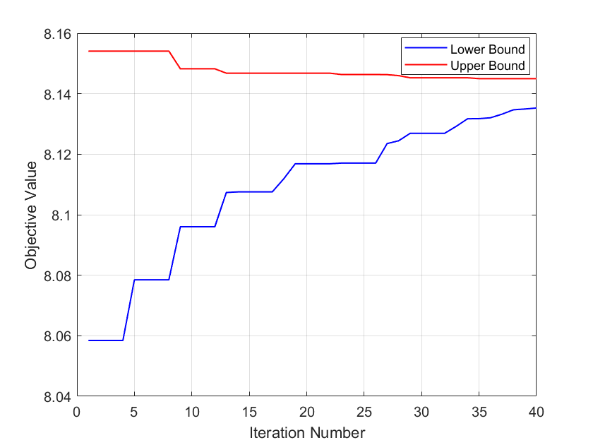
The convergence behavior of our proposed algorithm is shown in Fig. 1. In this simulation, we set the error tolerance , the power budget dB, and the weight parameter in Algorithm 1. The result is averaged over 10 Monte Carlo runs. It can be seen from Fig. 1 that the proposed B&B algorithm quickly converges to the global solution. In particular, the total number of iterations for the proposed algorithm to find the -optimal solution is (and the CPU time is seconds).
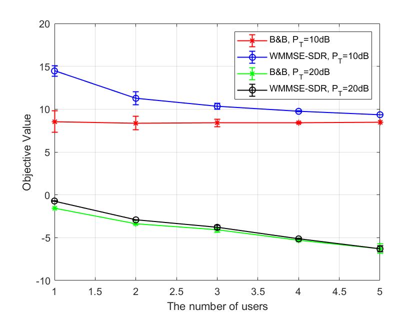
Furthermore, we evaluate the performance of an existing state-of-the-art algorithm [24] for solving the original nonconvex problem (7), which is called WMMSE-SDR. However, the WMMSE-SDR algorithm is only guaranteed to find a stationary point of problem (7). In Fig. 2, we show the impact of the communication user number on the objective value, with the power budget being set as 10 dB and 20 dB, respectively. It can be observed from Fig. 2 that the gap of the objective values at the solutions found by WMMSE-SDR and the proposed B&B algorithm becomes larger when the power increases. The results demonstrate the performance gain of the proposed global optimization algorithm over that of the local optimization algorithm.
References
- [1] I.-R. WP5D, “Draft new recommendation ITU-R M.[IMT.FRAMEWORK FOR 2030 AND BEYOND],” 2023.
- [2] M. L. Rahman, J. A. Zhang, X. Huang, Y. J. Guo, and R. W. Heath, “Framework for a perceptive mobile network using joint communication and radar sensing,” IEEE Transactions on Aerospace and Electronic Systems, vol. 56, no. 3, pp. 1926–1941, 2019.
- [3] B. Tan, Q. Chen, K. Chetty, K. Woodbridge, W. Li, and R. Piechocki, “Exploiting WiFi channel state information for residential healthcare informatics,” IEEE Communications Magazine, vol. 56, no. 5, pp. 130–137, 2018.
- [4] D. Ma, N. Shlezinger, T. Huang, Y. Liu, and Y. C. Eldar, “Joint radar-communication strategies for autonomous vehicles: Combining two key automotive technologies,” IEEE Signal Processing Magazine, vol. 37, no. 4, pp. 85–97, 2020.
- [5] Y. Xiong, F. Liu, Y. Cui, W. Yuan, T. X. Han, and G. Caire, “On the fundamental tradeoff of integrated sensing and communications under Gaussian channels,” IEEE Transactions on Information Theory, vol. 69, no. 9, pp. 5723–5751, 2023.
- [6] X. Song, J. Xu, F. Liu, T. X. Han, and Y. C. Eldar, “Intelligent reflecting surface enabled sensing: Cramér-Rao bound optimization,” IEEE Transactions on Signal Processing, vol. 71, pp. 2011–2026, 2023.
- [7] F. Liu, Y. Cui, C. Masouros, J. Xu, T. X. Han, Y. C. Eldar, and S. Buzzi, “Integrated sensing and communications: Toward dual-functional wireless networks for 6G and beyond,” IEEE Journal on Selected Areas in Communications, vol. 40, no. 6, pp. 1728–1767, 2022.
- [8] Z. He, W. Xu, H. Shen, D. W. K. Ng, Y. C. Eldar, and X. You, “Full-duplex communication for ISAC: Joint beamforming and power optimization,” IEEE Journal on Selected Areas in Communications, vol. 41, pp. 2920–2936, 2023.
- [9] F. Liu, Y.-F. Liu, A. Li, C. Masouros, and Y. C. Eldar, “Cramér-Rao bound optimization for joint radar-communication beamforming,” IEEE Transactions on Signal Processing, vol. 70, pp. 240–253, 2021.
- [10] F. Liu, Y.-F. Liu, C. Masouros, A. Li, and Y. C. Eldar, “A joint radar-communication precoding design based on Cramér-Rao bound optimization,” in Proceedings of IEEE Radar Conference, pp. 1–6, 2022.
- [11] X. Liu, T. Huang, N. Shlezinger, Y. Liu, J. Zhou, and Y. C. Eldar, “Joint transmit beamforming for multiuser MIMO communications and MIMO radar,” IEEE Transactions on Signal Processing, vol. 68, pp. 3929–3944, 2020.
- [12] Q. Shi, M. Razaviyayn, Z.-Q. Luo, and C. He, “An iteratively weighted MMSE approach to distributed sum-utility maximization for a MIMO interfering broadcast channel,” IEEE Transactions on Signal Processing, vol. 59, no. 9, pp. 4331–4340, 2011.
- [13] K. Shen and W. Yu, “Fractional programming for communication systems—Part I: Power control and beamforming,” IEEE Transactions on Signal Processing, vol. 66, no. 10, pp. 2616–2630, 2018.
- [14] M. Chiang, C. W. Tan, D. P. Palomar, D. O’neill, and D. Julian, “Power control by geometric programming,” IEEE Transactions on Wireless Communications, vol. 6, no. 7, pp. 2640–2651, 2007.
- [15] Z.-Q. Luo and S. Zhang, “Dynamic spectrum management: Complexity and duality,” IEEE Journal of Selected Topics in Signal Processing, vol. 2, no. 1, pp. 57–73, 2008.
- [16] P. C. Weeraddana, M. Codreanu, M. Latva-Aho, and A. Ephremides, “Weighted sum-rate maximization for a set of interfering links via branch and bound,” IEEE Transactions on Signal Processing, vol. 59, no. 8, pp. 3977–3996, 2011.
- [17] B. Matthiesen, C. Hellings, E. A. Jorswieck, and W. Utschick, “Mixed monotonic programming for fast global optimization,” IEEE Transactions on Signal Processing, vol. 68, pp. 2529–2544, 2020.
- [18] L. P. Qian, Y. J. Zhang, and J. Huang, “MAPEL: Achieving global optimality for a non-convex wireless power control problem,” IEEE Transactions on Wireless Communications, vol. 8, no. 3, pp. 1553–1563, 2009.
- [19] H. Tuy, F. Al-Khayyal, and P. T. Thach, “Monotonic optimization: Branch and cut methods,” in Essays and Surveys in Global Optimization, pp. 39–78, Springer, 2005.
- [20] L. Liu, R. Zhang, and K.-C. Chua, “Achieving global optimality for weighted sum-rate maximization in the K-user Gaussian interference channel with multiple antennas,” IEEE Transactions on Wireless Communications, vol. 11, no. 5, pp. 1933–1945, 2012.
- [21] C. Lu and Y.-F. Liu, “An efficient global algorithm for single-group multicast beamforming,” IEEE Transactions on Signal Processing, vol. 65, no. 14, pp. 3761–3774, 2017.
- [22] C. Lu, Y.-F. Liu, and J. Zhou, “An enhanced SDR based global algorithm for nonconvex complex quadratic programs with signal processing applications,” IEEE Open Journal of Signal Processing, vol. 1, pp. 120–134, 2020.
- [23] A. Schöbel and D. Scholz, “The theoretical and empirical rate of convergence for geometric branch-and-bound methods,” Journal of Global Optimization, vol. 48, pp. 473–495, 2010.
- [24] M. Zhu, L. Li, S. Xia, and T.-H. Chang, “Information and sensing beamforming optimization for multi-user multi-target MIMO ISAC systems,” EURASIP Journal on Advances in Signal Processing, vol. 2023, no. 1, p. 15, 2023.
- [25] B. Mats and O. Björn, “Optimum and suboptimum transmit beamforming,” in Handbook of Antennas in Wireless Communications, CRC press, 2018.
- [26] G. Pataki, “On the rank of extreme matrices in semidefinite programs and the multiplicity of optimal eigenvalues,” Mathematics of Operations Research, vol. 23, no. 2, pp. 339–358, 1998.
- [27] W.-K. Ma, J. Pan, A. M.-C. So, and T.-H. Chang, “Unraveling the rank-one solution mystery of robust miso downlink transmit optimization: A verifiable sufficient condition via a new duality result,” IEEE Transactions on Signal Processing, vol. 65, no. 7, pp. 1909–1924, 2017.
- [28] A. Mitsos, B. Chachuat, and P. I. Barton, “McCormick-based relaxations of algorithms,” SIAM Journal on Optimization, vol. 20, no. 2, pp. 573–601, 2009.
- [29] M. Grant and S. Boyd, “CVX: Matlab software for disciplined convex programming, version 2.1,” 2014.