Equilibrium with coordinate dependent diffusion: Comparison of different stochastic processes

Abstract

We investigate in this paper two different processes of scaling that map a multiplicative noise problem to an additive noise form. While by one method of scaling, at the over-damped limit, we obtain the equilibrium distribution of the Itô-process, by the other method we get the distribution of the Hänggi-Klimontovich (Isothermal) process. We compare the Itô-process to the Hänggi-Klimontovich (Isothermal) process in the light of these additive noise counterparts of the multiplicative noise problem to identify the underlying details of these processes. Where it comes out that the Itô-process is consistent with the standard physics of Brownian motion, the Hänggi-Klimontovich process, on the other hand, appears inconsistent with the fluctuation-dissipation relation. Present analysis provides us with insights related to coordinate-dependent diffusion which could be useful for application across discipline.

I Introduction

Thermodynamic equilibrium of a confined Brownian particle (BP) with coordinate-dependent diffusion needs to be understood for the possibility of its extensive application [1, 2, 3, 4, 5, 6, 7, 8, 9, 10] across disciplines. A BP near a wall or interface sees coordinate dependence of diffusion. The diffusivity of a particle gradually reduces from its bulk value as it approaches an interface [11]. The model of such a system is a stochastic differential equation (SDE) involving multiplicative noise. Solving such a model requires adoption of a particular convention for stochastic integrals depending upon the physical situation prevailing. N. G. van Kampen had elaborated in the ref.[12] of the need of understanding different conventions (e.g., Itô or Stratonovich) to correspond to different physical processes.

Although the method of handling such SDE as a process with uncorrelated noise was formulated by Kiyosi Itô [13, 14] many decades ago, there have been dilemma in the physics community in adopting the Itô-convention for equilibrium of a BP under coordinate dependent diffusion [15, 16, 17, 18, 19, 20, 21, 22, 23]. The apparent reason for this dilemma has been that, the distribution that follows from Itô-convention is not considered to be the Boltzmann distribution corresponding to a specified potential that confines the BP. The present paper takes a simple approach to demonstrate that this has been a misunderstanding. The Itô-distribution is completely consistent with Boltzmann distribution for thermal equilibrium when one is able to identify the emergence of additional states resulting from the coordinate dependence of diffusion.

The equilibrium distribution (probability density of position distribution in one dimension) that results from Itô-convention implemented to solve SDE with multiplicative noise modeling a confined BP with coordinate-dependent diffusivity $D(x)$ at temperature $T$ is of the form

$$\rho(x)=\frac{N}{D(x)}e^{-V(x)/k_{B}T},$$ (1)

where the conservative confining field is given by the potential function $V(x)$ and $N$ is a normalization constant. This distribution is apparently considered not to be of the Boltzmann distribution because of the fact that, the diffusivity ($D(x)$) is not in general known to feature in the Hamiltonian of the system. In what follows, we will refer to the distribution of the form given by Eq.(1) to be the Itô-type distribution.

The distribution that one considers as the thermodynamic equilibrium distribution for such a BP is of the from

$$\rho(x)=Me^{-V(x)/k_{B}T}$$ (2)

where $M$ is normalization constant. In what follows, we will refer this distribution (Eq.(2)), in the context of coordinate dependent diffusion to be HK-type distribution because it results from a Hänggi-Klimontovich process as well. The reason for such nomenclature - i.e. Itô/HK-type - is to avoid any confusion at the onset as to which one is the distribution corresponding to the Gibbs/Boltzmann measure for thermal equilibrium. It will be identified in this paper that although the Ito-type and HK-type processes appear to represent equilibrium distribution at the over-damped limit, however, the under-damped limit shows the problem with the HK-type process in terms of satisfying the fluctuation-dissipation relation (FDR).

The mapping to additive noise stochastic dynamics that we do in this paper for the Itô-process considers the time scale to be the one set my the relaxation time of Brownian motion i.e., $m_{0}/\Gamma(x)$ where $\Gamma(x)$ is the damping coefficient and $m_{0}$ is the mass of the particle. Holding of the FDR everywhere in space indicates $D(x)\Gamma(x)=k_{B}T$. Consideration of the velocity scale of the system to be its thermal (RMS velocity) $\sqrt{k_{B}T/m_{0}}$, dictates the relevant length scale of the system to be $\sqrt{k_{B}Tm_{0}}/\Gamma(x)$ which is coordinate dependent as the time scale itself.

On the contrary, mapping to the additive noise problem for the HK-type distribution is obtained by considering a coordinate dependent time scale $r_{0}^{2}/D(x)$ where $r_{0}$ is considered to be some uniform length scale over the whole space. It is shown that, with this scaling, one gets the HK-type distribution as the equilibrium distribution of the system in the over-damped limit. However, when one looks into the under-damped dynamics with this same scaling i.e., mass of the particle is taken into account, there appears a violation of the FDR. This happens because fixing the uniform length scale for the problem of coordinate-dependent diffusion makes the mass of the particle coordinate dependent which then affects the temperature locally. This problem is obviously not there for the mapping corresponding to the Itô-process.

The factor of $1/D(x)$ in the Itô-type distribution is identified to be proportional to the density of states appearing due to lifting of homogeneity of space by $D(x)$. This density of states corresponds to an entropy $S[D(x)]=k_{B}\log{\frac{D_{0}}{D(x)}}$, where $D_{0}$ is the bulk diffusion constant such that $D_{0}\geq D(x)$. This entropy could be understood to be due to the additional states associated with local diffusivity $D(x)<D_{0}$ [24]. These issues have been looked at from different perspective in the ref.s [25, 26, 24]. In the paper by Maniar and Bhattacharyay [27], a random walk model for coordinate dependent diffusion has been constructed using waiting time at points on a uniform lattice. That work had presented a crucial clue on the possibility of modelling coordinate dependent diffusion by local scaling of time which is practically utilized in the present paper for mapping to additive noise forms.

The plan of paper is the following: In the next section we revisit standard results related to Itô and HK-type conventions for clarity and give a schematic description of competing probability currents. Then we present the mapping and explore the microscopic reality of the Itô-type and HK-type distributions. This is followed by having a look at the under-damped case for the Itô-type process and an explanation to the additional entropy arising from coordinate dependence of diffusion. Then we compare the under-damped dynamics of the Itô- and HK-type processes. We end the paper with a short discussion.

II Revisiting different conventions

The Langevin equation, that generally considered as a model of a Brownian particle with coordinate dependent diffusivity $D(x)$, can be written in one-dimension for the over-damped case as

$$\frac{dx}{dt}=-\frac{1}{\Gamma(x)}\frac{\partial V(x)}{\partial x}+\sqrt{\frac{2k_{B}T}{\Gamma(x)}}\eta(t),$$ (3)

where the potential $V(x)$ confines the particle which has position coordinate $x$ at time $t$. The particle is in contact with a heat-bath at temperature $T$ and $k_{B}$ is the Boltzmann constant. In this equation, $\eta(t)$ is a Gaussian white noise of unit strength. We consider here the one-dimensional case for the sake of simplicity. In fact, coordinate dependence of $\Gamma(x)$ is due to presence of an interface where, for example, $x$-coordinate is the distance from the interface. On planes orthogonal to this coordinate ($x=$ constant) the damping should remain uniform. The diffusivity $D(x)$, in what follows, is always considered to obey the Stokes-Einstein relation $D(x)=\frac{k_{B}T}{\Gamma(x)}$.

The corresponding Fokker-Planck equation for the probability density to Eq.(3) in the case of a generalized Stratonovich process has the structure

$$\frac{\partial\rho(x,t)}{\partial t}=-\frac{\partial}{\partial x}\left(-\frac{\rho(x)D(x)}{k_{B}T}\frac{\partial V(x)}{\partial x}-\frac{\partial}{\partial x}D(x)\rho(x)+\alpha\rho(x)\frac{\partial}{\partial x}D(x)\right).$$ (4)

The constant factor $\alpha$ can take any value such that $0\leq\alpha\leq 1$. When $\alpha=0$, one has implemented the Itô convention - the stochastic noise is treated in a way such that it remains correlation-free. For $\alpha\neq 0$, one uses a generalized Stratonovich convention. The Stratonovich convention corresponds to $\alpha=\frac{1}{2}$, whereas $\alpha=1$, which considers the noise to be most correlated, is generally termed as the Hänggi-Klimontovich (Isothermal) process. The last term on the r.h.s of the above equation is generally referred to as the spurious drift term. It is a drift term whose origin is in the correlation of the noise. However, one may clearly see that, if the potential $V(x)$ considered renormalized to include this drift term, then, Eq.(4) represents a legitimate Itô-process even for non-zero $\alpha$.

For an equilibrium solution which is stationary, one has to implement the condition of detailed balance i.e. set the probability current density to zero. This results in the equation

$$-\frac{\rho(x)D(x)}{k_{B}T}\frac{\partial V(x)}{\partial x}+\alpha\rho(x)\frac{\partial}{\partial x}D(x)-\left(D(x)\frac{\partial}{\partial x}\rho(x)+\rho(x)\frac{\partial}{\partial x}D(x)\right)=0$$ (5)

Eq.(5) shows that, for an Itô-process ($\alpha=0$), the equilibrium distribution is of the form given in Eq.(1) (Itô-type). This is so, because of the presence of the additional diffusion current $-\rho(x)\frac{\partial}{\partial x}D(x)$ arising from the coordinate dependence of diffusivity. This additional diffusion current is convention independent and is always there in any case.

Similarly, for $\alpha=1$, the distribution will come out to be the one given by Eq.(2) (HK-type) which, in general, is considered to be the distribution describing the equilibrium of the system. In this case, one gets the distribution of the HK-type because of the complete cancellation of the additional diffusion current $-\rho(x)\frac{\partial}{\partial x}D(x)$ by the spurious drift current $\rho(x)\frac{\partial}{\partial x}D(x)$. For $\alpha\neq 1$ the distribution will be somewhere between the Itô- and HK-type. In the present paper we would focus on the cases $\alpha=0$ and $\alpha=1$.

To understand the origin of these two distinct equilibrium solutions in particular, one needs to pay attention to the origin of probability current densities. To relate various probability current densities to the corresponding local and global broken isotropy of space an analogous jump process to diffusion, which is the continuum limit of such jump processes, would be very useful. Fig.1 shows schematic diagram to relate the additional diffusion current density $-\rho(x)\frac{\partial D(x)}{\partial x}$ and the spurious drift $\rho(x)\frac{\partial D(x)}{\partial x}$ (for $\alpha=1$) to the broken (isotropy) symmetries. The additional diffusion current arising from the global broken symmetry due to the coordinate dependent diffusivity can be understood from Fig.1(a).

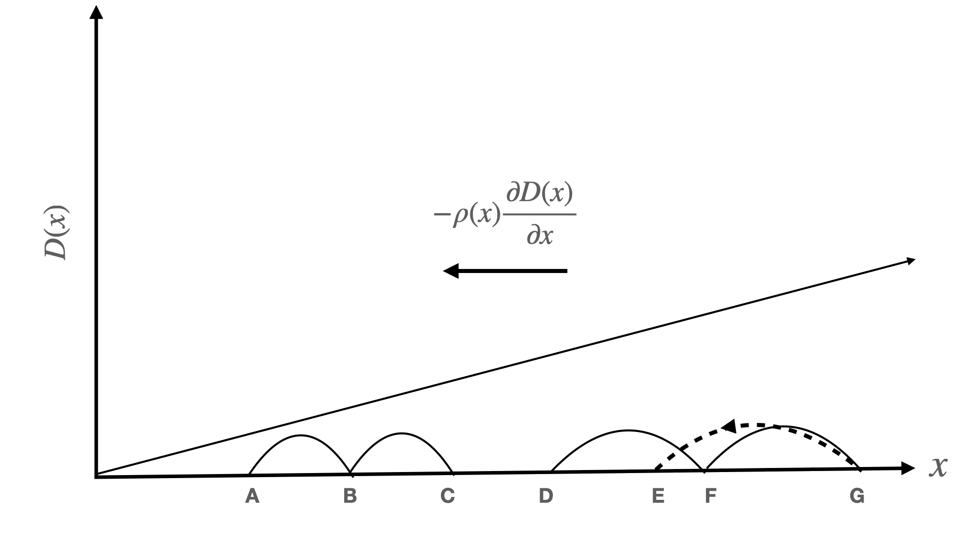
(a) No correlated noise (Itô-convention)

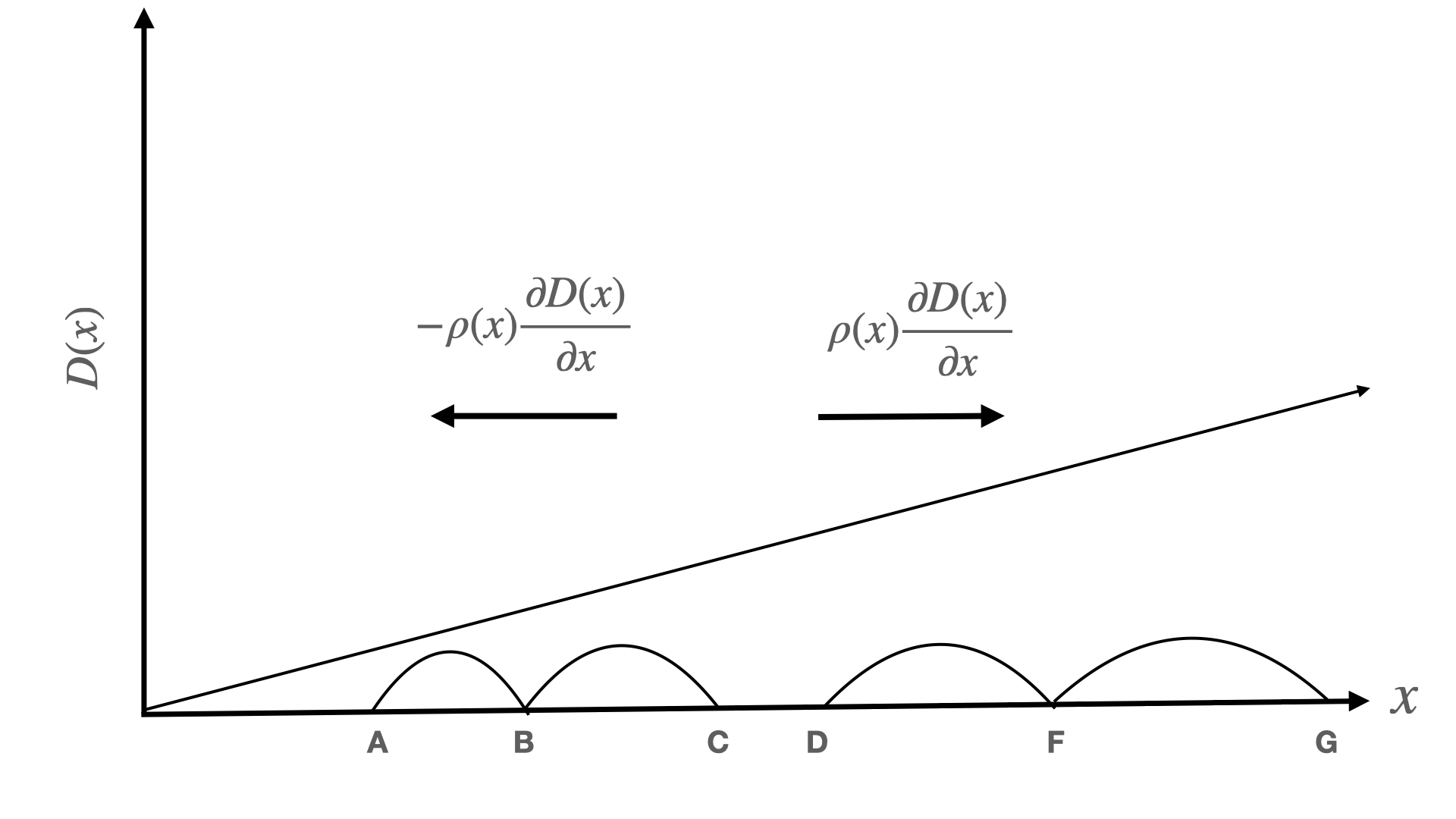
(b) Correlated noise (Hänggi-Klimontovich convention)

Figure 1: Schematic diagram to understand the origin of additional currents in the presence of diffusivity gradient.

Consider the diffusivity profile to increase linearly with the coordinate $x$ as in Fig1.(a) and (b). Since the diffusive transport must be locally isotropic, a particle makes equal jumps from the position B (say) to left/right (A/C) respectively. It would also make equal jumps on either side of F (at a different position) to D and G however with a bigger jump size. This would be so because the diffusivity at F is bigger than that at B. This is the idea of global symmetry breaking due to the presence of diffusivity gradient. Imagine the situation where the particle at F has first jumped to G (right) and then has jumped backward (dashed line) to E. These pair of jumps would produce a current in a direction opposite to the diffusion gradient. Now, over an ensemble, all such pairs could be formed giving rise to the additional diffusion current $-\rho(x)\frac{\partial D(x)}{\partial x}$. This is not a drift current because it has not arisen out of local breaking of isotropy at a point in space which happens in the presence of a force. This additional diffusion current will always be there irrespective of Itô or Stratonovich or generalized Stratonovich convention is implemented. Presence of this additional diffusion current under coordinate dependent diffusion results in the Itô-type distribution as in Eq.(1).

On top of this additional diffusion current, there will be present the (spurious) drift current due to implementation of (generalized) Stratonovich convention. To understand the origin of that drift current, consider the schematic diagram of Fig.1(b) where we have in mind $\alpha=1$. In the generalized Stratonovich convention, noise is anticipating i.e., the particle makes bigger jump towards the increasing diffusivity than what it does on the other side. This happens on top of the fact that jump sizes at a higher diffusivity region are bigger than those in the regions of smaller diffusivity. The asymmetry in jump on two sides breaks the local isotropy at each point in space a way akin to what the presence of a force does to the system. This breakdown of the local isotropy would produce the drift current (spurious) for anticipating noises in the direction of the diffusivity gradient and that would exactly balance the additional diffusion current when $\alpha=1$. This is what one achieves by implementing the Hänggi-Klimontovich convention for $\alpha=1$.

However, the fallacy of Stratonovich or generalized Stratonovich approachs is in the fact that, these approaches in effect take into account presence of additional drift current without making it count in the potential. Therefore, identification of the HK-type distribution resulting from such approaches as the equilibrium distribution is a source of confusion. Consideration of correlated noise in these contexts is a disguise that does not make any sense in the context of equilibrium. A force has to appear as a conservative force with a well defined confinement for one to identify thermodynamic equilibrium. To look inside these issues, if one is able to make a mapping of the problems to corresponding additive noise forms, one would be able to distinguish the underlying physics because the additive noise problem is quite well understood in general.

III Mapping Itô-process to SDE with additive noise

III.1 over-damped case

The Langevin dynamics evolved to update the position of a BP is of the form

$$\frac{dx}{dt}=-\frac{1}{\Gamma(x)}\frac{\partial V(x)}{\partial x}+\sqrt{\frac{2k_{B}T}{\Gamma(x)}}\times\eta(t),$$ (6)

where $\eta(t)$ is a Gaussian white noise of unit strength and $\eta(t)\sim 1/\sqrt{dt}$.

III.1.1 Itô-type distribution

Note that, the dimension of $\Gamma(x)$ is actually mass/time, which obviously suggests a natural (physical) way of scaling time so that $t\to\infty$ limit remains well defined with respect to the characteristic time scale $m_{0}\Gamma(x)^{-1}$ where $m_{0}$ is the mass of the particle. The scale of the mass could be assumed to be that of a micrometer-radius particle of density equivalent to that of water at room temperature. This gives the order of magnitude of $\Gamma(x)=6\pi\eta r_{0}\simeq 10^{-8}$ kg/s where the dynamic viscosity $\eta\simeq 10^{-3}$ Pa-s and the radius of the particle $r_{0}=10^{-6}$ m. To work with this natural scale of time, multiplying Eq.(6) on both sides by $m_{0}$. Choosing the dimensionless time such that $d\tau=\frac{\Gamma(x)dt}{m_{0}}$ and a change of variable $d\phi(x)=\Gamma(x)dx$, one gets

$$\frac{d\phi(x)}{d\tau}=-m_{0}\frac{\partial V[\phi(x)]}{\partial\phi(x)}+\sqrt{2k_{B}Tm_{0}}\times\eta(\tau).$$ (7)

This local joint rescaling of time and space does not change the momentum of the particle i.e. $\frac{d\phi(x)}{d\tau}\equiv m_{0}\frac{dx}{dt}$ and could be imagined as a symmetry of diffusion process in the absence of the diffusivity showing up in the Hamiltonian. That, this is an exact mapping of an Itô-process to an additive noise SDE would be revealed by the resulting equilibrium distribution. The time is locally scaled by the natural relaxation time of the BP where change of coordinate gets automatically suggested by the rescaling of time keeping the velocity unaltered. Because the momentum remains same on rescaling, the $\eta(\tau)$ is a white noise of unit strength on these scales. The above equation could also be brought to a dimention-less form

$$\frac{d\phi^{\prime}(x)}{d\tau}=-\frac{\partial}{\partial\phi^{\prime}(x)}\frac{V[\phi^{\prime}(x)]}{k_{B}T}+\sqrt{2}\times\eta(\tau),$$ (8)

where $\phi^{\prime}(x)=\phi(x)/\sqrt{m_{0}k_{B}T}$.

This dynamics at $\tau\to\infty$ admits the stationary equilibrium distribution of the variable $\phi(x)$ under the confinement with a probability density

$$\rho[\phi(x)]=Ne^{-\frac{V[\phi(x)]}{k_{B}T}},$$ (9)

where the normalization constant $N$ has the dimension of inverse momentum. Probability to find the particle at $\phi(x)$ within an interval of $d\phi(x)$ is, therefore, given by

$$P[\phi(x)]=Ne^{-\frac{V[\phi(x)]}{k_{B}T}}d\phi(x)\equiv N^{\prime}e^{-\frac{V(x)}{k_{B}T}}\Gamma(x)dx.$$ (10)

Keeping in mind the fluctuation-dissipation relation, one gets the probability density for the distribution of position of the particle as

$$\rho(x)=M\frac{D_{0}}{D(x)}e^{-\frac{V(x)}{k_{B}T}},$$ (11)

where $M=\frac{N^{\prime}k_{B}T}{D_{0}}$, which is the new normalization constant is of dimension inverse length. A micrometer-size particle of equivalent density as water in room temperature has a mass $m_{0}\sim 10^{-14}$ Kg.

Therefore, the time at which the particle will come to equilibrium with the confinement is of the order $\tau\geq m_{0}/\Gamma_{0}\simeq 10^{-14}/10^{-8}=10^{-6}$ s or smaller where the typical value of the $\Gamma_{0}$ is considered to be that in the bulk which increases as the BP approaches an interface. Note that, the time scale $m_{0}/\Gamma(x)$ is the local time scale of the BP to relax to equilibrium once some local kick to it by the bath degrees of freedom has changed its velocity. This is the underlying physics of the Brownian motion.

However, the particle to see its equilibrium density profile in accordance with the nature of confinement (additional source of inhomogeneity of space), it needs to see the whole confining profile. This takes a much bigger time than the time scale $m_{0}/\Gamma(x)$ to actually sample the stationary equilibrium profile of the probability density in relation to the confinement. When in the process of exploring that confined space by Brownian motion, the BP has always relaxed to the local equilibrium at position $x$ at the time scale $m_{0}/\Gamma(x)$ is the underlying physics. Scaling of space and time that maps the problem to homogeneous Brownian motion utilizes this fact.

III.1.2 HK-type distribution

Let us look at another scaling leading to a mapping to homogeneous Brownian motion which would be equivalent to the Hänggi-Klimontovich process. Note that, Eq.(6) can also be written as

$$\frac{r_{0}^{2}}{D(x)}\frac{dx}{dt}=-\frac{r_{0}^{2}}{D(x)}\frac{1}{\Gamma(x)}\frac{\partial V(x)}{\partial x}+\frac{r_{0}^{2}}{D(x)}\sqrt{2D(x)}\times\eta(t),$$ (12)

where $r_{0}$ is a length scale, which on rescaling to dimensionless time $\tau^{\prime}\to\frac{D(x)}{r_{0}^{2}}t$ and $x^{\prime}=x/r_{0}$ will give the homogeneous equation

$$\frac{dx^{\prime}}{d\tau^{\prime}}=-\frac{\partial}{\partial x^{\prime}}\frac{V(x^{\prime})}{k_{B}T}+\sqrt{2}\times\eta(\tau^{\prime}).$$ (13)

This system reaches equilibrium with the HK-type distribution

$$\rho(x)=Ne^{-\frac{V(x)}{k_{B}T}}$$ (14)

at a time $t>\tau^{\prime}$ where $N$ is the normalization constant.

The ratio of the units $\tau^{\prime}$ to that of $\tau$ is

$$\frac{{r_{0}^{2}}/{D(x)}}{{m_{0}}/{\Gamma_{0}}}=\frac{r_{0}^{2}\Gamma_{0}^{2}}{m_{0}k_{B}T}.$$ (15)

The length scale at which $\tau^{\prime}$ is comparable to $\tau$ (local relaxation time) is of nanometer order which is comparable to the thermal length scale $\sqrt{m_{0}k_{B}T}/\Gamma_{0}$. Looking at the over-damped dynamics, up to this level, the two processes are appearing to be equivalent.

III.2 under-damped (Itô-type) case

The set of coupled SDE modeling the under-damped (general) evolution of a particle of mass $m_{0}$ under confinement with coordinate-dependent diffusion is

$$\frac{dx}{dt}=v$$

$$m_{0}\frac{dv}{dt}=-m_{0}\zeta(x)v-\left(\frac{\partial V(x)}{\partial x}\right)+\sqrt{2k_{b}Tm_{0}\zeta(x)}\times\eta(t).$$ (16)

In these equations, $\Gamma(x)=m\zeta(x)$ where $\zeta(x)^{-1}$ is the time scale at which the BP comes to equilibrium with the bath being disturbed at $t=0$ (say).

With the variable $d\phi(x)=\zeta(x)dx$ and naturally scaled dimensionless time $\tau=\zeta(x)dt$ already defined, it is now trivial to check that the dynamics takes an additive noise form. The set of linear SDE looks as

$$\frac{d\phi(x)}{d\tau}=v$$

$$m_{0}\frac{dv}{d\tau}=-m_{0}v-\frac{\partial V[\phi(x)]}{\partial\phi(x)}+\sqrt{2k_{B}Tm_{0}}\times\eta({\tau}).$$ (17)

This dynamics would admit an equilibrium probability density at $\tau\to\infty$, given by

$$\rho[\phi(x)]=Ne^{-\frac{V[\phi(x)]}{k_{B}T}}e^{-\frac{m_{0}v^{2}}{2k_{B}T}}.$$ (18)

The over-damped limit - $m\to 0$ and $\zeta\to\infty$, such that $\Gamma(x)$ remains finite - will make one get the distribution given by Eq.(9). This is so, because, the BP relaxes to equilibrium at a time-scale $\zeta^{-1}$ which is much smaller than any finite $\tau$ when the dynamics is over-damped (slow dynamics). Following the procedure shown, it is now trivial to identify the equilibrium density of position $x$ and velocity $v$ to be

$$\rho(x,v)=M\frac{D_{0}}{D(x)}e^{-\frac{V(x)}{k_{B}T}}e^{-\frac{m_{0}v^{2}}{2k_{B}T}}.$$ (19)

This distribution is consistent with the Boltzmann form (Gibbs distribution in other words) on identification of the density of states $D_{0}/D(x)$. The distribution can now be rewritten as

$$\rho(x,v)=M^{\prime}e^{-\frac{1}{k_{B}T}\left(H(x,p)-T[k_{B}\log{\frac{D_{0}}{D(x)}]}\right)},$$ (20)

where $H(x,p)$ is the Hamiltonian of the system with $p=m_{0}v$ in the present case. The entropy corresponding to the degeneracy of a state originating from coordinate dependence of Brownian motion

$$S[D(x)]=k_{B}\log{\frac{D_{0}}{D(x)}},$$ (21)

is positive definite because $D_{0}\geq D(x)$. The choice of the constant $D_{0}$ might appear arbitrary, however, this makes every sense within the scope of the model. Keeping in mind that, it is the difference in entropy that matters, the arbitrariness is somewhat not that serious under the reasonable assumption that $T\to 0$ is equivalent to $D(x)\to D_{0}$ as quickly as $D_{0}\to 0$. Therefore, physical effect of the presence of interfaces through hydrodynamics should vanish at this limit. At finite temperature, $D(x)\to 0$ can result in a considerable contribution to the entropy.

The physical origin of this entropy under coordinate dependent diffusion could be easily understood from an analogy of quantum mechanics. The role played by the Planck’s constant $h$ in quantum mechanics is the same as that played by the diffusivity $D$ in classical diffusion. Where $h$ is the smallest phase space volume within which one cannot be precise in quantum mechanics and hence $h$ denotes the phase volume corresponding to a single state in one dimension, the same is true of $D$ and it defines the phase volume in the (position-velocity) phase space for the BP.

In the bulk, where the diffusivity is a constant ($D_{0}$) this count does not matter because it is the same at all positions. However, this count of available states in the units of diffusivity $D(x)<D_{0}$ starts increasing as one reaches an interface. This is why, the density of states goes as $D_{0}/D(x)$ as the BP comes near an interface as the diffusivity gets correspondingly reduced from its bulk value. This is a consequence of the fact that the BP starts relaxing much faster than that in bulk with an increase in $\zeta(x)$ near an interface.

Obviously, the free energy of the system is

$$F=H(x,p)-TS[D(x)],$$ (22)

which would now dictate the thermodynamics of the system. Thermodynamics of BP undergoing coordinate dependent diffusion has a bigger phase space. It is wonderful to see that the Itô-convention automatically takes care of the presence of these additional fluctuations present in the model.

III.3 Comparison of under-damped dynamics

So far, looking at the over-damped dynamics the two methods appear to be on par, however, the problem with the scaling of Hänggi-Klimontovich process would be evident when we go with the same for under-damped case. If we apply the same scaling as is done in Eq.(22) to Eq.(15), we get

$$\frac{dx^{\prime}}{d\tau^{\prime}} = v^{\prime}$$

$$m_{0}\frac{dv^{\prime}}{d\tau^{\prime}} = -\frac{r_{0}^{2}k_{B}T}{D(x)^{2}}v^{\prime}-\frac{r_{0}^{2}}{D(x)^{2}}\frac{\partial V(x^{\prime})}{\partial x^{\prime}}+\frac{r_{0}^{2}k_{B}T}{D(x)^{2}}\sqrt{2}\times\eta({\tau^{\prime}}),$$ (23)

where $v^{\prime}=\frac{r_{0}}{D(x)}v$, which is dimension-less.

Eq.(22), as compared to Eq.(16), introduces an explicit mass scale $m_{T}(x)=\frac{r_{0}^{2}k_{B}T}{D(x)^{2}}$ in the presence of which the fluctuation-dissipation relation (FDR) gets manifestly broken. Note that, Eq.(22) becomes dimensionally equivalent to Eq.(16) when we multiply (22) by a velocity scale $v_{0}=\sqrt{\frac{k_{B}T}{m_{0}}}$ and absorb that in the velocity $v^{\prime\prime}$ to make it dimension full and replace $x^{\prime}$ by $x^{\prime\prime}=\sqrt{\frac{k_{B}T}{m_{0}}}x^{\prime}$ to make it dimensionally similar to $\phi(x)$. Now, with this adjustment Eq.(22) takes the form

$$m_{0}\frac{dv^{\prime\prime}}{d\tau^{\prime}}=-\frac{r_{0}^{2}k_{B}T}{D(x)^{2}}v^{\prime\prime}-\frac{r_{0}^{2}}{D(x)^{2}}\frac{k_{B}T}{m_{0}}\frac{\partial V(x^{\prime\prime})}{\partial x^{\prime\prime}}+\frac{r_{0}^{2}k_{B}T}{D(x)^{2}}\sqrt{\frac{2k_{B}T}{m_{0}}}\times\eta({\tau^{\prime}}).$$ (24)

The above equation can only go in the form of Eq.(16) when $\frac{r_{0}^{2}k_{B}T}{D(x)^{2}}=m_{0}$, which is never possible with $D(x)$ being coordinate dependent and $r_{0}$ being a constant. Therefore, only for homogeneous diffusion this scaling would work (keeping the temperature of the system unaffected) with the typical choice of $x_{0}=\frac{\sqrt{m_{0}k_{B}T}}{\Gamma_{0}}$. Whereas, in the presence of coordinate dependent diffusion, where $\frac{r_{0}^{2}k_{B}T}{D(x)^{2}}\neq m_{0}$, the correct length scale naturally comes out to be $x_{0}(x)=\frac{\sqrt{m_{0}k_{B}T}}{\Gamma(x)}$, as opposed to a uniform length scale, which underlies the scaling for the Itô-process as has been shown. The breakdown of the FDR in the under-damped case would be revealed in the over-damped scenario in effectively making temperature a coordinate-dependent quantity although one fixes the energy scale to $k_{B}T$. This would happen due to the coordinate dependence of the mass scale $\frac{r_{0}^{2}k_{B}T}{D(x)^{2}}$.

IV discussion

We have used two distinct ways of mapping Langevin dynamics with multiplicative noise to additive forms. Equilibrium results obtained from the respective mapping in the over-damped case interestingly match two competing stochastic processes (Itô and Hänggi-Klimontovich) considered as competing equilibrium solutions for the multiplicative noise problem. However, the over-damped case does not reveal the whole picture on the basis of which the apparent equilibrium could be ascertained. It turns out that, the mapping used in the case of Itô-process remains completely consistent with the FDR when implemented to the under-damped case. However, the other mapping corresponding to HK-type distribution manifestly breaks the FDR when applied to the under-damped dynamics. Result of this breaking of the FDR in the case of the Hänggi-Klimontovich case would effectively entail a coordinate-dependent temperature in this case even in the over-damped limit where the mass is practically hidden. This would happen because of the consideration of uniform length scale where the time scale is determined by the coordinate dependent diffusivity.

The Itô-type or the Itô distribution is completely consistent with the natural scales of diffusion sticking to which is essential for coordinate-dependent diffusion. It provides the equilibrium state in the presence of coordinate-dependent damping/diffusion with the FDR intact. Other important message that follows from the present analysis is that, even in the over-damped limit of the dynamics, the mass plays an important role by helping select natural scales consistent with the FDR. Moreover, after having got the mapping to additive noise form the controversy related to the multiplicative noise problem possibly is resolved and one can avoid the multiplicative noise models for equilibrium of such systems.

References

- Roussel and Roussel [2004] C. J. Roussel and M. R. Roussel, Reaction–diffusion models of development with state-dependent chemical diffusion coefficients, Progress in biophysics and molecular biology 86, 113 (2004).
- Barik and Ray [2005] D. Barik and D. S. Ray, Quantum state-dependent diffusion and multiplicative noise: a microscopic approach, Journal of Statistical Physics 120, 339 (2005).
- Sargsyan et al. [2007] V. Sargsyan, Y. V. Palchikov, Z. Kanokov, G. Adamian, and N. Antonenko, Coordinate-dependent diffusion coefficients: Decay rate in open quantum systems, Physical Review A 75, 062115 (2007).
- Chahine et al. [2007] J. Chahine, R. J. Oliveira, V. B. Leite, and J. Wang, Configuration-dependent diffusion can shift the kinetic transition state and barrier height of protein folding, Proceedings of the National Academy of Sciences 104, 14646 (2007).
- Best and Hummer [2010] R. B. Best and G. Hummer, Coordinate-dependent diffusion in protein folding, Proceedings of the National Academy of Sciences 107, 1088 (2010).
- Lai et al. [2014] Z. Lai, K. Zhang, and J. Wang, Exploring multi-dimensional coordinate-dependent diffusion dynamics on the energy landscape of protein conformation change, Physical Chemistry Chemical Physics 16, 6486 (2014).
- Berezhkovskii and Makarov [2017] A. M. Berezhkovskii and D. E. Makarov, Communication: Coordinate-dependent diffusivity from single molecule trajectories, The Journal of chemical physics 147, 201102 (2017).
- Foster et al. [2018] D. A. Foster, R. Petrosyan, A. G. Pyo, A. Hoffmann, F. Wang, and M. T. Woodside, Probing position-dependent diffusion in folding reactions using single-molecule force spectroscopy, Biophysical journal 114, 1657 (2018).
- Ghysels et al. [2017] A. Ghysels, R. M. Venable, R. W. Pastor, and G. Hummer, Position-dependent diffusion tensors in anisotropic media from simulation: oxygen transport in and through membranes, Journal of chemical theory and computation 13, 2962 (2017).
- Yamilov et al. [2014] A. G. Yamilov, R. Sarma, B. Redding, B. Payne, H. Noh, and H. Cao, Position-dependent diffusion of light in disordered waveguides, Physical review letters 112, 023904 (2014).
- Faucheux and Libchaber [1994] L. P. Faucheux and A. J. Libchaber, Confined brownian motion, Physical Review E 49, 5158 (1994).
- Van Kampen [1981] N. G. Van Kampen, Itô versus stratonovich, Journal of Statistical Physics 24, 175 (1981).
- Itô [1942] K. Itô, Differential equations determining a markoff process (original japanese: Zen-koku sizyo sugaku danwakai-si) journ, Pan-Japan Math Coll (1942).
- Itô [1986] K. Itô, Kiyosi itô selected papers, dw stroock and srs varadhan eds (1986).
- Sancho et al. [1982] J. Sancho, M. S. Miguel, and D. Dürr, Adiabatic elimination for systems of brownian particles with nonconstant damping coefficients, Journal of Statistical Physics 28, 291 (1982).
- Lau and Lubensky [2007] A. W. Lau and T. C. Lubensky, State-dependent diffusion: Thermodynamic consistency and its path integral formulation, Physical Review E 76, 011123 (2007).
- Sokolov [2010] I. M. Sokolov, Itô, stratonovich, hänggi and all the rest: The thermodynamics of interpretation, Chemical Physics 375, 359 (2010).
- Tupper and Yang [2012] P. Tupper and X. Yang, A paradox of state-dependent diffusion and how to resolve it, Proceedings of the Royal Society A: Mathematical, Physical and Engineering Sciences 468, 3864 (2012).
- Sancho [2011] J. M. Sancho, Brownian colloidal particles: Ito, stratonovich, or a different stochastic interpretation, Physical Review E 84, 062102 (2011).
- Farago and Grønbech-Jensen [2014a] O. Farago and N. Grønbech-Jensen, Fluctuation–dissipation relation for systems with spatially varying friction, Journal of Statistical Physics 156, 1093 (2014a).
- Farago and Grønbech-Jensen [2014b] O. Farago and N. Grønbech-Jensen, Langevin dynamics in inhomogeneous media: Re-examining the itô-stratonovich dilemma, Physical Review E 89, 013301 (2014b).
- Leibovich and Barkai [2019] N. Leibovich and E. Barkai, Infinite ergodic theory for heterogeneous diffusion processes, Physical Review E 99, 042138 (2019).
- Mannella and McClintock [2022] R. Mannella and P. V. McClintock, Itô versus stratonovich: 30 years later, The Random and Fluctuating World: Celebrating Two Decades of Fluctuation and Noise Letters , 9 (2022).
- Bhattacharyay [2022] A. Bhattacharyay, Physical interpretation of it^ o–distribution on the basis of local measurement of diffusion, arXiv preprint arXiv:2209.00995 (2022).
- Bhattacharyay [2019] A. Bhattacharyay, Equilibrium of a brownian particle with coordinate dependent diffusivity and damping: Generalized boltzmann distribution, Physica A: Statistical Mechanics and its Applications 515, 665 (2019).
- Bhattacharyay [2020] A. Bhattacharyay, Generalization of stokes–einstein relation to coordinate dependent damping and diffusivity: an apparent conflict, Journal of Physics A: Mathematical and Theoretical 53, 075002 (2020).
- Maniar and Bhattacharyay [2021] R. Maniar and A. Bhattacharyay, Random walk model for coordinate-dependent diffusion in a force field, Physica A: Statistical Mechanics and its Applications 584, 126348 (2021).