Distributionally Robust Transfer Learning

Abstract

Many existing transfer learning methods rely on leveraging information from source data that closely resembles the target data. However, this approach often overlooks valuable knowledge that may be present in different yet potentially related auxiliary samples. When dealing with a limited amount of target data and a diverse range of source models, our paper introduces a novel approach, Distributionally Robust Optimization for Transfer Learning (TransDRO), that breaks free from strict similarity constraints. TransDRO is designed to optimize the most adversarial loss within an uncertainty set, defined as a collection of target populations generated as a convex combination of source distributions that guarantee excellent prediction performances for the target data. TransDRO effectively bridges the realms of transfer learning and distributional robustness prediction models. We establish the identifiability of TransDRO and its interpretation as a weighted average of source models closest to the baseline model. We also show that TransDRO achieves a faster convergence rate than the model fitted with the target data. Our comprehensive numerical studies and analysis of multi-institutional electronic health records data using TransDRO further substantiate the robustness and accuracy of TransDRO, highlighting its potential as a powerful tool in transfer learning applications.

1 Introduction

Transfer learning stands as a pivotal concept in the realm of statistical and machine learning due to its immense importance and transformative potential (Torrey and Shavlik, 2010). It allows models trained on existing datasets to leverage their knowledge and expertise when confronted with a new target population. Transfer learning enables models to generalize and adapt their acquired knowledge to novel challenges, making them more versatile and generalizable. Transfer learning has potentials to rapidly develop generalizable model for new target populations, addressing scarcity of clinical data (Desautels et al. (2017), Gligic et al. (2020), Laparra et al. (2021)). An example of such analysis is to develop a rare-disease mortality prediction model in a target hospital with limited labels, by aid of abundant EHR data from other large hospitals (Desautels et al., 2017).

Leveraging existing labeled data from multiple sources to derive to optimally derive a precise prediction model for a new target population, however, is highly challenging in the presence of heterogeneity among the sources and between the target and source population. To ensure useful information can be borrowed from the source samples and avoid negative transfer, one of the key assumptions for traditional transfer learning models is that the target model and some of the source models need to possess a certain level of similarity. For example, both the transGLM (Tian and Feng, 2022a) and transLASSO (Li et al., 2022) models require the recovery of the set of transferrable source sites, which share similar parameters with the target measured by the $l_{1}$-norm. The distance between the parameters of these transferrable sources and that of the target needs to be quite small so that introducing source data in their algorithms can help sharpen the estimation error rate. However, informative sources might get dropped because of the stringent requirement of the transferrable set and the natural heterogeneity for data collected from different sources. It would be much preferred to construct a prediction model without imposing such similarity conditions, but it is still capable of leveraging the underlying relationship between the target and sources.

On the other hand, assuming the target comes from a mixture of source populations, group distributional robust optimization (Sagawa et al. (2019), Hu et al. (2018), Meinshausen and Bühlmann (2015); Guo (2023); Wang et al. (2023)) has proven to be a robust prediction model when analyzing the source data without the target outcomes. Specifically, given $L$ groups of source distributions $\{\mathbb{P}^{(l)}:=(\mathbb{P}_{X}^{(l)},\mathbb{P}_{Y|X}^{(l)})\}_{1\leq l\leq L}$, when the target labels are not available and the target model $\mathbb{Q}_{Y|X}$ is allowed to differ from any of $\{\mathbb{P}^{(l)}_{Y|X}\}_{1\leq l\leq L}$, $\mathbb{Q}_{Y|X}$ is in general not identifiable. Instead of estimating the true $\mathbb{Q}_{Y|X}$, group DRO models assume $\mathbb{Q}_{Y|X}$ is a mixture of $\{\mathbb{P}^{(l)}_{Y|X}\}_{1\leq l\leq L}$ and define an uncertainty set $\mathcal{C}_{0}$ as any mixture of these sources, i.e.,

$$\mathcal{C}_{0}=\left\{\mathbb{Q}=(\mathbb{T}_{X},\mathbb{T}_{Y|X}):\mathbb{T}_{Y|X}=\sum_{l=1}^{L}q_{l}\cdot\mathbb{P}^{(l)}_{Y|X}\;\text{with}\;q\in\Delta_{L}\right\}.$$ (1)

where $\triangle_{L}=\left\{q\in\mathbb{R}^{L}:\sum_{l=1}^{L}q_{l}=1,\min_{l}q_{l}\geq 0\right\}$ is the $(L-1)$-dimensional probability simplex. Given a model family $\Theta$ and a loss function $l:\Theta\times(\mathcal{X}\times\mathcal{Y})\to\mathbb{R}_{+}$, group DRO minimizes the worst-case expected loss over the uncertainty set $\mathcal{C}_{0}$:

$$\min_{\theta\in\Theta}\left\{\sup_{\mathbb{T}\in\mathcal{C}_{0}}\mathbf{E}_{(X,Y)\sim\mathbb{T}}\left[l(\theta;X,Y)\right]\right\}$$ (2)

The uncertainty set encodes the possible test distributions that might contain $\mathbb{Q}_{Y|X}$ and that we want our model to perform well on. Choosing a general family such as $\mathcal{C}_{0}$, group DRO is effective in improving the prediction model’s generalizability to a wide set of distribution shifts but can also lead to overly pessimistic models which optimize for implausible worst-case distributions. Therefore, when a limited number of target labels are indeed available in our setting, we aim to construct a realistic uncertainty set of possible test distributions closer to $Q_{Y|X}$ without being overly conservative.

Maximin effect (Meinshausen and Bühlmann, 2015) is the solution to a specific group DRO problem under the linear assumption. It adopts the same uncertainty set $\mathcal{C}_{0}$ and introduces a new loss function defined as the residual variance if measured against the baseline of residual variance under a constant 0 prediction:

$$\min_{\theta\in\Theta}\left\{\sup_{\mathbb{T}\in\mathcal{C}_{0}}\mathbf{E}_{(X,Y)\sim\mathbb{T}}\left[(Y-X^{\intercal}\theta)^{2}-Y^{2}\right]\right\}$$ (3)

Meinshausen and Bühlmann (2015) has been shown that under the linear structure assumption, the maximin effect is equivalent to the convex combination of the source model that has the minimum distance to the origin. Specifically, when a variable has heterogeneous effects scattered around zero across multiple sources, its maximin effect will shrink to the baseline 0 due to the design of the loss function. Such a shrinkage is often appealing when no target labels are at hand and we would like to avoid doing worse than a zero constant prediction. Yet, under our model setting, the zero baseline may be a poor choice which ignores information in the existing target labels. Therefore, having a smaller residual variance compared to the zero baseline does not necessarily guarantee a better prediction performance. We would instead consider a linear mixture of both sources and the target model with the lowest training loss as an informative baseline. The linear combination idea of sources resembles Zhang et al. (2023), but we do not assume partially shared parameters across sources and the target. Also, our baseline is more flexible to drill for shared knowledge in the presence of heterogeneity between sources and target an, whereas the estimator of Zhang et al. (2023) will degenerate to the target-only estimator if there are no covariates with identical effects.

In this paper, we consider the construction of distributionally robust transfer-learning prediction model (TransDRO) with a small number of target labels and abundant yet distinct source data. Inspired by the design of DRO and group DRO models, the main idea of TransDRO is to incorporate the distributional uncertainty of the target data into the optimization process. The key operational step is to minimize the adversarial loss defined over a possible class of target distributions on the convex hull of sources with small prediction errors. Such a constrained uncertainty set not only leverages the relationship between sources and the target, but also makes full use of target labels and guides TransDRO effect toward the interested target problem. Consequently, the distributional robustness is defined on a smaller class with a higher chance of containing the true target model. We also construct a new loss function incorporating an informative baseline, which is again guided by the target labels and further improves the prediction performance. Owing to the target guidance introduced to the uncertainty set and the loss function, TransDRO serves as a bridge connecting the field of DRO models and transfer learning. Nice transferability and generalizability, as a result, can be both expected in the TransDRO estimator. Another unique merit of TransDRO resides in the privacy protection for source data, as it only requires the transfer of summary-level statistics across source sites. Under the linear assumption, we have shown in the theoretical analysis that TransDRO effect can be easily identified and has a nice interpretation as a weighted average of source models closest to the baseline. More advantages for TransDRO namely a faster convergence rate as well as smaller estimation errors have been proved rigorously and exploited in extensive simulation study as well as real data analysis.

2 TransDRO model

2.1 Setting

We focus on the setting that we have access to $L$ groups of training data sets $\{(Y^{(l)},X^{(l)})\}_{1\leq l\leq L}$. We assume that these $L$ training data sets might be generated from heterogeneous source populations. For the $l$-th source population with $1\leq l\leq L$, we use $\mathbb{P}_{X}^{(l)}$ and $\mathbb{P}^{(l)}_{Y|X}$ to respectively denote the corresponding covariate and conditional outcome distributions of the $l$-th source data, that is, the data $\{X^{(l)}_{i},Y^{(l)}_{i}\}_{1\leq i\leq n_{l}}$ are i.i.d. generated as

$$X^{(l)}_{i}{\;\mathrel{\overset{i.i.d}{\scalebox{1.5}[1.0]{$\sim$}}}\;}\mathbb{P}_{X}^{(l)},\quad Y^{(l)}_{i}\mid X^{(l)}_{i}{\;\mathrel{\overset{i.i.d}{\scalebox{1.5}[1.0]{$\sim$}}}\;}\mathbb{P}^{(l)}_{Y|X}\quad\text{for}\quad 1\leq i\leq N_{l},$$ (4)

For the target population, we consider the data $\{X^{\mathbb{Q}}_{i},Y^{\mathbb{Q}}_{i}\}_{1\leq i\leq N_{\mathbb{Q}}}$ being generated as as

$$X^{\mathbb{Q}}_{i}{\;\mathrel{\overset{i.i.d}{\scalebox{1.5}[1.0]{$\sim$}}}\;}\mathbb{Q}_{X},\quad Y^{\mathbb{Q}}_{i}\mid X^{\mathbb{Q}}_{i}{\;\mathrel{\overset{i.i.d}{\scalebox{1.5}[1.0]{$\sim$}}}\;}\mathbb{Q}_{Y|X}\quad\text{for}\quad 1\leq i\leq N_{\mathbb{Q}}.$$ (5)

We focus on the setting where only the covariates $\{X^{\mathbb{Q}}_{i}\}_{1\leq i\leq N_{\mathbb{Q}}}$ and a limited number of the outcome variables $\{Y^{\mathbb{Q}}_{i}\}_{1\leq i\leq n}$ are observed ($n\ll N_{\mathbb{Q}}$). This commonly occurs in applications where we would like to build a prediction model for a target population with very few outcome labels but have access to related source populations with plentiful outcome labels.

2.2 Model definition and identification

Given $L$ groups of source distributions $\{\mathbb{P}^{(l)}:=(\mathbb{P}_{X}^{(l)},\mathbb{P}_{Y|X}^{(l)})\}_{1\leq l\leq L}$, and a target distribution $\mathbb{Q}:=(\mathbb{Q}_{X},\mathbb{Q}_{Y|X})$, TransDRO model focuses on the mixture of source distributions and aims to minimize the worse-case expected loss over a transferrable uncertainty set:

$$\mathcal{C}(\tau)=\left\{\mathbb{T}=(\mathbb{Q}_{X},\mathbb{T}_{Y|X})\in\mathcal{C}_{0}:\mathbf{E}_{\mathbb{Q}}(\mathbf{E}_{\mathbb{T}_{Y|X}}Y-Y)^{2}\leq\mathbf{E}_{\mathbb{Q}}(\mathbf{E}_{\mathbb{Q}_{Y|X}}Y-Y)^{2}+\tau\right\},$$

with $\mathcal{C}_{0}$ defined in (1) and $\tau\geq 0$ is a user-specific constant. The parameter $\tau$ controls the size of $\mathcal{C}(\tau)$ as well as the largest distance between any $\mathbb{T}$ in $\mathcal{C}(\tau)$ and $\mathbb{Q}$ in terms of the prediction error. The smaller $\tau$ gets, the fewer elements $\mathcal{C}(\tau)$ would contain, while the closer each element becomes to $\mathbb{Q}$.

Given a model family $\Theta$, we then define a new loss function as the squared residual under a prediction model $f(X;\theta)$ against that under a baseline model $f(X;\theta_{\mathrm{init}})$:

$$l(\theta;X,Y,\theta_{\mathrm{init}}) =\left[Y-f(X;\theta)\right]^{2}-\left[Y-f(X;\theta_{\mathrm{init}})\right]^{2},$$ (6)

where $\theta_{\mathrm{init}}$ is any initial estimator with zero as the default choice. Note that under the linear structure assumption for $f$ and by taking $\theta_{\mathrm{init}}$ as zero, (6) becomes the loss used in the maximin problem (Meinshausen and Bühlmann, 2015). TransDRO chooses a flexible baseline $\theta_{\mathrm{init}}$ instead of a constant zero since it is more beneficial to compete with a baseline closer to the target outcomes when the purpose is to train a nice prediction model for the target. On the other hand, if the goal shifts from transferability to generalizability, we can select a less informative $\theta_{\mathrm{init}}$ in terms of the current target data. In general, both the parameter $\tau$ from the uncertainty set and the initial baseline $\theta_{\mathrm{init}}$ embedded in the loss balance the emphasis on the prediction accuracy and model robustness. The corresponding TransDRO problem becomes

$$\theta_{\mathrm{TransDRO}}(\theta_{\mathrm{init}},\tau)=\min_{\theta\in\Theta}\left\{\mathcal{R}(\theta,\theta_{\mathrm{init}}):=\sup_{\mathbb{T}\in\mathcal{C}(\tau)}\mathbf{E}_{(X,Y)\sim\mathbb{T}}\left\{\left[Y-f(X;\theta)\right]^{2}-\left[Y-f(X;\theta_{\mathrm{init}})\right]^{2}\right\}\right\}$$ (7)

In this paper, we focus on the linear models for source sites as well as the target:

$$Y_{i}^{(l)}=\left[X_{i}^{(l)}\right]^{\intercal}b^{(l)}+\epsilon^{(l)}_{i}\,\,\text{ where }\mathbf{E}\left(\epsilon_{i}^{(l)}|X_{i}^{(l)}\right)=0,\,\,\mathbf{E}\left[(\epsilon_{i}^{\mathbb{P}})^{2}|X_{i}^{\mathbb{Q}}\right]=\sigma_{\mathbb{P}}^{2}.$$ (8)

$$Y_{i}^{\mathbb{Q}}=\left[X_{i}^{\mathbb{Q}}\right]^{\intercal}\beta^{*}+\epsilon_{i}^{\mathbb{Q}}\,\,\text{ where }\mathbf{E}\left(\epsilon_{i}^{\mathbb{Q}}|X_{i}^{\mathbb{Q}}\right)=0,\,\,\mathbf{E}\left[(\epsilon_{i}^{\mathbb{Q}})^{2}|X_{i}^{\mathbb{Q}}\right]=\sigma_{\mathbb{Q}}^{2}.$$ (9)

The prediction model also follows a linear structure that $f(X;\beta)=X^{\intercal}\beta$ where $\beta\in\mathbb{R}^{p}$. Define $B=(b^{(1)},...,b^{(L)})\in\mathbb{R}^{p\times L}$. Under (8) and (9), when we fix $\mathbb{Q}_{X}$, data $(Y,X)$ following distribution in $\mathcal{C}(\tau)$ will share the linear form $Y=X^{\intercal}b+\epsilon$ where $\mathbf{E}\left(\epsilon|X\right)=0$. $b=\sum_{l=1}^{L}\gamma_{l}\cdot b^{(l)}=B\gamma$ is a convex combination of source coefficients with the weight $\gamma=(\gamma_{1},...,\gamma_{L})^{\intercal}$ satisfying:

$$\gamma\in\mathcal{S}(\tau):=\{\gamma\in\Delta_{L}:\mathbf{E}_{(X,Y)\sim\mathbb{Q}}(X^{\intercal}B\gamma-Y)^{2}\leq\sigma_{\mathbb{Q}}^{2}+\tau\}.$$ (10)

Note that $\mathcal{S}(\tau)$ is a convex set for $\gamma$, which is designed to ease the optimization problem. The expected loss function under the distribution $\mathbb{T}\in\mathcal{C}(\tau)$ w.r.t an initial baseline $\beta_{\mathrm{init}}$ can be further simplified as:

$$\mathbf{E}_{(X,Y)\sim\mathbb{T}}\left[l(\beta;X,Y,\beta_{\mathrm{init}})\right] =\mathbf{E}_{(X,Y)\sim\mathbb{T}}\left[\left(Y-X^{\intercal}\beta\right)^{2}-\left(Y-X^{\intercal}\beta_{\mathrm{init}}\right)^{2}\right]$$ (11)

$$=\mathbf{E}_{X\sim\mathbb{Q}_{X}}\left[\beta^{\intercal}XX^{\intercal}\beta-\beta_{\mathrm{init}}^{\intercal}XX^{\intercal}\beta_{\mathrm{init}}+2\left(\beta_{\mathrm{init}}-\beta\right)^{\intercal}XX^{\intercal}B\gamma\right],$$

where $\gamma\in\mathcal{S}(\tau)$. Define $\Sigma_{\mathbb{Q}}$ to be the population Gram matrix $\mathbf{E}_{X\sim\mathbb{Q}_{X}}\left[XX^{\intercal}\right]$. The TransDRO problem in (7) under the linear model can be re-written as:

$$\beta_{\mathrm{TransDRO}}(\beta_{\mathrm{init}},\tau)=\operatorname*{arg\,min}_{\beta\in\mathbb{R}^{p}}\max_{\gamma\in\mathcal{S}(\tau)}\left\{\beta^{\intercal}\Sigma_{\mathbb{Q}}\beta+2\left(\beta_{\mathrm{init}}-\beta\right)^{\intercal}\Sigma_{\mathbb{Q}}B\gamma\right\}$$ (12)

The definition of $\beta_{\mathrm{TransDRO}}(\beta_{\mathrm{init}},\tau)$ can be interpreted from a two-side game perspective: for each model $\beta$, the counter agent searches over the weight set $\mathcal{S}(\tau)$ and generates the most challenging target population with parameter $b=B\gamma(\gamma\in\mathcal{S}(\tau))$. $b$ lies close to $\beta^{*}$ due to the prediction error constraint. Then $\beta_{\mathrm{TransDRO}}(\beta_{\mathrm{init}},\tau)$ guarantees the optimal prediction accuracy for such an adversarially generated target population. Also, it explains the generalizability of $\beta_{\mathrm{TransDRO}}(\beta_{\mathrm{init}},\tau)$ since it is not designed to optimize the predictive performance for a single target population, but over many possible target populations. When there is no confusion, we write $\beta_{\mathrm{TransDRO}}(\beta_{\mathrm{init}},\tau)$ as $\beta_{\mathrm{TransDRO}}$.

In the following theorem, we will show how to identify the TransDRO effect. The proof will be shown in the appendix.

Theorem 1.

Suppose that the linear model (8) for source data and (9) for target data holds. Then the TransDRO effect $\beta_{\mathrm{TransDRO}}$ defined in (12) is given by:

$$\beta_{\mathrm{TransDRO}}=\sum_{l=1}^{L}\gamma_{\mathrm{TransDRO}}^{(l)}b^{(l)}=B\gamma_{\mathrm{TransDRO}}\quad\text{with}\quad\gamma_{\mathrm{TransDRO}}=\operatorname*{arg\,min}_{\gamma\in\mathcal{S}(\tau)}\gamma^{\intercal}\Gamma_{\mathrm{init}}\gamma$$ (13)

where $\left[\Gamma_{\mathrm{init}}\right]_{l,k}=[b^{(l)}-\beta_{\mathrm{init}}]^{\intercal}\Sigma_{\mathbb{Q}}[b^{(k)}-\beta_{\mathrm{init}}]$.

Essentially, the equivalent expression for the TransDRO effect in (13) is a convex combination of source coefficients. To obtain the corresponding weight $\gamma_{\mathrm{TransDRO}}$, we only need to solve a convex optimization problem within a convex constraint set $\mathcal{S}(\tau)$. Minimizing the objective function $g(\gamma)=\gamma^{\intercal}\Gamma_{\mathrm{init}}\gamma$ means to find a $\gamma\in\mathcal{S}(\tau)$ such that $B\gamma$ is ‘closest’ to $\beta_{\mathrm{init}}$. Note that if $\beta_{\mathrm{init}}$ lies inside $\{\beta:\beta=B\gamma,\gamma\in\mathcal{S}(\tau)\}$, then $\beta_{\mathrm{TransDRO}}$ is equal to $\beta_{\mathrm{init}}$.

Compared (13) with the identification of the maximin effect:

$$\beta_{\text{maximin}}=\sum_{l=1}^{L}\gamma_{\text{maximin}}^{(l)}b^{(l)}=B\gamma_{\text{maximin}}\quad\text{with}\quad\gamma_{\text{maximin}}=\operatorname*{arg\,min}_{\gamma\in\Delta_{L}}\gamma^{\intercal}\Gamma\gamma$$

where $\Gamma_{l,k}=[b^{(l)}-0]^{\intercal}\Sigma_{\mathbb{Q}}[b^{(k)}-0]$, there are two types of unique guidance introduced to the TransDRO effect. First, instead of searching over the entire convex hull spanned by the support of $\{b^{(l)}\}_{1\leq l\leq L}$, TransDRO limits the range to a small area (i.e., $\mathcal{S}(\tau)$) that is closer to $\beta^{*}$. Second, within the constraint set, rather than locating the effect nearest to zero, TransDRO finds the closest point to $\beta_{\mathrm{init}}$. Even though $\beta_{\mathrm{TransDRO}}$ is typically different from the best linear approximation derived from the true $\beta^{*}$, depending on the relative location of $\beta_{\mathrm{init}}$ and $\beta^{*}$ as well as the size of $\mathcal{S}(\tau)$, we show in the following proposition that $\beta_{\mathrm{TransDRO}}$ can approach $\beta^{*}$.

Proposition 1.

Suppose that the linear model (8) for source data and (9) for target data holds. Also assume there exists $\gamma^{*}$ such that $\beta^{*}=B\gamma^{*}$ and $\Sigma_{\mathbb{Q}}$ is invertible. Either $\tau\to 0$ or $\beta_{\mathrm{init}}\to\beta^{*}$ guarantees that $\beta_{\mathrm{TransDRO}}\to\beta^{*}$.

Remark 1.

Define

$$\widetilde{\gamma}^{*}=\operatorname*{arg\,min}_{\gamma\in\Delta_{L}}(\beta^{*}-B\gamma)^{\intercal}\Sigma_{\mathbb{Q}}(\beta^{*}-B\gamma)$$ (14)

and $\widetilde{\beta}^{*}=B\widetilde{\gamma}^{*}$, which is the closest source mixture to the target model. If $\beta^{*}$ does not come from the mixture of $\{b^{(l)}\}_{1\leq l\leq L}$, then the minimum $\tau$ that guarantees a non-empty $\mathcal{S}(\tau)$ has the format as follows:

$$\alpha(=\tau_{\text{min}}) :=\min_{\gamma\in\Delta_{L}}\mathbf{E}_{X\sim\mathbb{Q}_{X}}\left[X^{\intercal}B\gamma-X^{\intercal}\beta^{*}-\epsilon_{\mathbb{Q}}\right]^{2}-\sigma_{\mathbb{Q}}^{2}$$ (15)

$$=(\beta^{*}-B\widetilde{\gamma}^{*})^{\intercal}\Sigma_{\mathbb{Q}}(\beta^{*}-B\widetilde{\gamma}^{*})$$

where the second equation derives from the assumption that $\epsilon_{\mathbb{Q}}$ is independent of $X^{\mathbb{Q}}$. Under this case, when $\tau\to\alpha$, $\beta_{\mathrm{TransDRO}}\to\widetilde{\beta}^{*}$ no matter what $\beta_{\mathrm{init}}$ is.

2.3 Estimation

In this section, we establish the estimation method for $\beta_{\mathrm{TransDRO}}$. We first construct a sample version $\widehat{\mathcal{S}}(\tau)$ for $\mathcal{S}(\tau)$ in (10) (i.e., estimate $b^{(1)},...,b^{(L)}$ and $\sigma_{\mathbb{Q}}^{2}$). Also, different versions of $\widehat{\beta}_{\mathrm{init}}$ as well as the corresponding plug-in estimator $\widehat{\Gamma}_{\mathrm{init}}$ will be given. Then we can obtain $\widehat{\gamma}_{\mathrm{TransDRO}}$ by solving a sample version of the convex optimization problem in (13). The final $\widehat{\beta}_{\mathrm{TransDRO}}$ is equal to $\widehat{B}\cdot\widehat{\gamma}_{\mathrm{TransDRO}}$.

2.3.1 Construction of $\widehat{\mathcal{S}}(\tau)$

To construct $\widehat{\mathcal{S}}(\tau)$, we first estimate $b^{(1)},...,b^{(L)}$ by Lasso separately:

$$\widehat{b}^{(l)}=\operatorname*{arg\,min}_{\beta\in\mathbb{R}^{p}}\left[\frac{1}{N_{l}}\sum_{i=1}^{N_{l}}\left(Y_{i}^{(l)}-(X_{i}^{(l)})^{\intercal}\beta\right)^{2}+\lambda^{(l)}\|\beta\|_{1}\right]$$

Denote $\widehat{B}=\left(\widehat{b}^{(1)},...,\widehat{b}^{(L)}\right)$. A naive estimator for $\sigma_{\mathbb{Q}}^{2}$ is first to split the target data into two parts $(Y_{s_{1}}^{\mathbb{Q}},X_{s_{1}}^{\mathbb{Q}})$ and $(Y_{s_{2}}^{\mathbb{Q}},X_{s_{2}}^{\mathbb{Q}})$. Use the first part to estimate $\beta^{*}$ by

$$\widehat{\beta}_{s_{1}}=\operatorname*{arg\,min}_{\beta}\frac{1}{n_{s_{1}}}\|Y_{s_{1}}^{\mathbb{Q}}-X_{s_{1}}^{\mathbb{Q}}\beta\|_{2}^{2}+\lambda_{s_{1}}\|\beta\|_{1}$$ (16)

Then use the plug-in estimator for $\sigma_{\mathbb{Q}}^{2}$ with the second part:

$$\widehat{\sigma}_{\mathbb{Q}}^{2}=\frac{1}{n_{s_{2}}}\|Y_{s_{2}}^{\mathbb{Q}}-X_{s_{2}}^{\mathbb{Q}}\widehat{\beta}_{s_{1}}\|_{2}^{2}$$ (17)

However, given the small number of target data, $\widehat{\sigma}_{\mathbb{Q}}^{2}$ might be quite unstable. On the other hand, if $\beta^{*}$ is a convex combination of $\{b^{(l)}\}_{l=1,...,L}$, we can construct another estimator for $\beta^{*}$ by $\widehat{B}\widehat{\gamma}_{s_{1}}$ where

$$\widehat{\gamma}_{s_{1}}=\operatorname*{arg\,min}_{\gamma\in\Delta_{L}}\frac{1}{n_{s_{1}}}\|Y_{s_{1}}^{\mathbb{Q}}-X_{s_{1}}^{\mathbb{Q}}\widehat{B}\gamma\|_{2}^{2}$$ (18)

Then the corresponding estimator for $\sigma_{\mathbb{Q}}^{2}$ has the format:

$$\widehat{\sigma}^{2}_{\text{source}}=\frac{1}{n_{s_{2}}}\|Y_{s_{2}}^{\mathbb{Q}}-X_{s_{2}}^{\mathbb{Q}}\widehat{B}\widehat{\gamma}_{s_{1}}\|_{2}^{2}$$ (19)

When the convex combination assumption is violated, then $\widehat{\sigma}^{2}_{\text{source}}$ becomes a estimator for $\operatorname*{arg\,min}_{\gamma\in\triangle_{L}}\mathbf{E}_{(X,Y)\sim\mathbb{Q}}\left((Y-X^{\intercal}B\gamma)^{2}\right)=\alpha+\sigma_{\mathbb{Q}}^{2}$ which is larger than $\sigma_{\mathbb{Q}}^{2}$. Therefore, to combine all information at hand, we estimate $\sigma_{\mathbb{Q}}^{2}$ as $\min\left\{\widehat{\sigma}_{\mathbb{Q}}^{2},\widehat{\sigma}_{\text{source}}^{2}\right\}$.

Notice that if the true target effect $\beta^{*}$ is far away from any convex combination of source effects, then $\mathcal{S}(\tau)$ in (10) is likely to be empty when we choose a small $\tau$. The same issue applies to the sample version $\widehat{\mathcal{S}}(\tau)=\left\{\gamma\in\Delta_{L}:\frac{1}{n}\|Y^{\mathbb{Q}}-X^{\mathbb{Q}}\widehat{B}\gamma\|_{2}^{2}\leq\min\left\{\widehat{\sigma}_{\mathbb{Q}}^{2},\widehat{\sigma}_{\text{source}}^{2}\right\}+\tau\right\}$. To solve this issue, we treat the target as one source site and expand $B=(b^{(1)},...,b^{(L)})$ to $B_{0}=(b^{(0)},b^{(1)},...,b^{(L)})$ where $b^{(0)}:=\beta^{*}$. Then the convex combination assumption for $\beta^{*}$ is always true as $\beta^{*}=B_{0}\gamma^{*}_{0}$ at least holds for one $\gamma^{*}_{0}=(1,0,...,0)$. As a consequence, we can estimate $\mathcal{S}(\tau)$ as:

$$\widehat{\mathcal{S}}(\tau)=\left\{\gamma_{0}\in\Delta_{L+1}:\frac{1}{n_{s_{2}}}\|Y^{\mathbb{Q}}_{s_{2}}-X^{\mathbb{Q}}_{s_{2}}\widehat{B}_{0}\gamma_{0}\|_{2}^{2}\leq\min\{\widehat{\sigma}_{\mathbb{Q}}^{2},\widehat{\sigma}_{\text{source}}^{2}\}+\tau\right\}$$ (20)

2.3.2 Choice of $\widehat{\beta}_{\mathrm{init}}$

$\widehat{\beta}_{\mathrm{init}}$ is expected to have a relatively good prediction performance on the target data so that the TransDRO effect optimizing the worst-case reward competing to the baseline can benefit from. The original maximin paper selected a zero baseline which might be desirable when no outcome data is available on the target site. However, the zero baseline might guide the TransDRO effect to the wrong direction in terms of predicting outcomes for target data, especially for variables with strong signals. Another choice is to utilize the target data and construct:

$$\widehat{\beta}_{\text{targetLasso}}=\operatorname*{arg\,min}_{\beta\in\mathbb{R}^{p}}\left[\frac{1}{n}\|Y^{\mathbb{Q}}-X^{\mathbb{Q}}\beta\|_{2}^{2}+\lambda\|\beta\|_{1}\right]$$

Yet, such an estimator might suffer from a large prediction error in the high-dimensional setting due to a small sample size for the target outcomes.

To leverage the ample source data and similarity between sources and target, and inspired by the construction of $\widehat{\gamma}_{s_{1}}$ in (18), we design a baseline estimator as a weighted average of $\{\widehat{b}^{(0)},\widehat{b}^{(1)},...,\widehat{b}^{(L)}\}$ that minimizes the prediction error. Specifically, we use LASSO with the first half of the split data to construct $\widehat{b}^{(0)}_{s_{1}}$ and the corresponding $\widehat{B}_{0,s_{1}}=(\widehat{\beta}_{s_{1}},\widehat{b}^{(1)},...,\widehat{b}^{(L)})$. Then utilize the second half to obtain the weight $\widehat{\gamma}_{0,s_{1}}$:

$$\widehat{\gamma}_{0,s_{1}}=\operatorname*{arg\,min}_{\gamma_{0}\in\Delta_{L+1}}\frac{1}{n_{s_{2}}}\|Y_{s_{2}}^{\mathbb{Q}}-X_{s_{2}}^{\mathbb{Q}}\widehat{B}_{0,s_{1}}\gamma_{0}\|_{2}^{2}$$

Similarly, we get $\widehat{B}_{0,s_{2}}$ and $\widehat{\gamma}_{0,s_{2}}$ by applying the cross-fitting strategy. The final weighted baseline takes the average of the two:

$$\widehat{\beta}_{\mathrm{init}}=\left(\widehat{B}_{0,s_{1}}\widehat{\gamma}_{0,s_{1}}+\widehat{B}_{0,s_{2}}\widehat{\gamma}_{0,s_{2}}\right)/2.$$

Note that both $\widehat{B}_{0,s_{1}}\times\widehat{\gamma}_{0,s_{1}}$ and $\widehat{B}_{0,s_{2}}\times\widehat{\gamma}_{0,s_{2}}$ lie in the convex hull spanned by the support of $\{\widehat{b}^{(l)}\}_{l=0,1,...,L}$ since $\widehat{\gamma}_{0,s_{1}}\in\Delta_{L+1}$ and $\widehat{\gamma}_{0,s_{2}}\in\Delta_{L+1}$. We can also expand the range of $\Delta_{L+1}$ to be an affine hull or a linear hull, given some prior knowledge about the relationship between $\{b^{(l)}\}_{1\leq l\leq L}$ and $\beta^{*}$. For example, if it is believed that there are some sources with opposite signs of effect compared to $\beta^{*}$, it may be better to assign a negative weight instead of dropping them entirely. Weighted average baselines with bounded and/or positive conditions (e.g., $\{\zeta_{+}:\zeta_{+,0}\in[0,1],0\leq\zeta_{+,l}\leq 1\text{ for }l=1,...,L\}$) are also implemented in the simulation study.

The reason for trying multiple types of linear combinations of $\widehat{B}_{0}$ for $\widehat{\beta}_{\mathrm{init}}$ is to see how weights from baselines guide the TransDRO effect to different directions, though the TransDRO effect itself can only be a convex combination of sources (and target if treated one source site). Note that $\widehat{\beta}_{\mathrm{init}}$’s are not guaranteed to lie in the estimated constraint set $\widehat{\mathcal{S}}_{0}(\tau)$. Therefore the resulting $\widehat{\beta}_{\mathrm{TransDRO}}(\widehat{\beta}_{\mathrm{init}},\tau)$ does not degenerate to $\widehat{\beta}_{\mathrm{init}}$.

3 Theoretical Analysis

3.1 Model Assumptions

Before presenting the main theorems, we introduce the assumptions for the TransDRO model.

Assumption 1.

For $1\leq l\leq L$, the regression coefficient $b^{(l)}$ is $k_{l}$- sparse. $\{X_{i}^{(l)},Y_{i}^{(l)}\}_{1\leq i\leq N_{l}}$ are i.i,d random variables, where $X_{i}^{(l)}\in\mathbb{R}^{p}$ is sub-gaussian with $\Sigma^{(l)}=\mathbf{E}[X_{i}^{(l)}(X_{i}^{(l)})^{\intercal}]$ satisfying $c_{0}\leq\lambda_{\text{min}}(\Sigma^{(l)})\leq\lambda_{\text{max}}(\Sigma^{(l)})\leq C_{0}$ for two positive constants $C_{0}>c_{0}>0$. The error $\epsilon_{i}^{(l)}$ is sub-gaussian with $\mathbf{E}[\epsilon_{i}^{(l)}|X_{i}^{(l)}]=0$ and $\mathbf{E}[(\epsilon_{i}^{(l)})^{2}|X_{i}^{(l)}]=\sigma_{l}^{2}$.

Assumption 2.

The regression coefficient $\beta^{*}$ is $k$-sparse. The target data $\{X_{i}^{\mathbb{Q}},Y_{i}^{\mathbb{Q}}\}_{1\leq i\leq n}$ are i.i.d samples drawn from $\mathbb{P}^{(l)}$, where the sub-gaussian $X_{i}^{\mathbb{Q}}\in\mathbb{R}^{p}$ has the second moment $\Sigma_{\mathbb{Q}}=\mathbf{E}[X_{i}^{\mathbb{Q}}(X_{i}^{\mathbb{Q}})^{\intercal}]$ satisfying $c_{1}\leq\lambda_{\text{min}}(\Sigma^{\mathbb{Q}})\leq\lambda_{\text{max}}(\Sigma_{\mathbb{Q}})\leq C_{1}$ for two positive constants $C_{1}>c_{1}>0$. $X_{i}^{\mathbb{Q}}$ can also be expressed in the form of $X_{i}^{\mathbb{Q}}=\Sigma_{\mathbb{Q}}^{\frac{1}{2}}Z_{i}$ where $Z_{i}\in\mathbb{R}^{p}$ is a sub-gaussian random vector of mean 0 and an identity covariance matrix. The target error $\epsilon_{i}^{\mathbb{Q}}$ also satisfies $\mathbf{E}[\epsilon_{i}^{\mathbb{Q}}|X_{i}^{(l)}]=0$ and $\mathbf{E}[(\epsilon_{i}^{\mathbb{Q}})^{2}|X_{i}^{(l)}]=\sigma_{\mathbb{Q}}^{2}$. $\epsilon_{i}^{\mathbb{Q}}$ is independent of $Z_{j}$ for any $i$ and $j$.

Assumption 1 and assumption 2 are commonly assumed for the theoretical analysis of high-dimensional linear models. The positive definite $\Sigma^{(l)}$ and the sub-gaussianity of $X_{i}^{(l)}$ guarantee the restricted eigenvalue condition with a high probability. The sub-gaussian errors are generally required for the theoretical analysis of the Lasso estimator in high dimensions.

Assumption 3.

For $0\leq l\leq L$, with data $(X^{(l)},Y^{(l)})$ drawn from $\mathbb{P}^{(l)}$ and $(X^{\mathbb{Q}},Y^{\mathbb{Q}})$ from $\mathbb{Q}$, the estimator $\widehat{b}^{(l)}$ for $b^{(l)}$ satisfies that with probability larger than $1-\delta(n)$ where $\delta(n)\to 0$,

$$\max\{\frac{1}{n}(\widehat{b}^{(l)}-b^{(l)})^{\intercal}\left[X^{\mathbb{Q}^{\intercal}}X^{\mathbb{Q}}\right](\widehat{b}^{(l)}-b^{(l)}),||\widehat{b}^{(l)}-b^{(l)}||_{2}^{2}\}\lesssim\frac{k_{l}\log p}{N_{l}}\sigma_{l}^{2}$$ (21)

$$\|(\widehat{b}^{(l)}-b^{(l)})_{S^{c}_{l}}\|\leq C^{(l)}_{0}\|(\widehat{b}^{(l)}-b^{(l)})_{S_{l}}\|$$ (22)

where $S_{l}=supp(b^{(l)})$ and $C_{0}^{(l)}>0$. $l=0$ denotes the target site. $b_{0}=\beta^{*}$ and $\mathbb{P}^{(0)}=\mathbb{Q}$.

3.2 Theoretical Property

We first show the upper bound for the estimation error of $X^{\mathbb{Q}}\beta^{*}$ using the TransDRO estimator $\widehat{\beta}_{\mathrm{TransDRO}}$ that falls into the constraint set $\widehat{S}_{0}(\tau)$ defined in (20). The proof of Theorem 23 is deferred to Appendix.

Theorem 2.

Under assumption 1, 2 and 3, if we suppose that the linear models (8) and (9) hold, when $n_{s_{1}}\asymp n_{s_{2}}\asymp n$, with probability larger than $1-\zeta(n)$ where $\zeta(n)\to 0$,

$$\frac{1}{n_{s_{2}}}\|X_{s_{2}}^{\mathbb{Q}}(\beta^{*}-\widehat{\beta}_{TransDRO})\|_{2}^{2} \lesssim{\color[rgb]{1,0,0}\tau}+\frac{\sigma_{\mathbb{Q}}^{2}(L+1)}{n}+\min\left\{\frac{k_{0}\log p}{n},\,\,{\color[rgb]{1,.5,0}4\alpha}+\max_{l\in\{1,...,L\}}\frac{k_{l}\log p}{N_{l}}\right\},$$ (23)

where $\alpha$ is defined as the distance between $\beta^{*}$ and its best linear approximation $B\widetilde{\gamma}^{*}$ in (15).

Remark 2.

Under the case when $L\ll n$ and $\tau$ is in the order of $\frac{1}{n}$, the estimation error is dominated by $\frac{k_{0}\log p}{n}$ and $4\alpha+\max_{l\in\{1,...,L\}}\frac{k_{l}\log p}{N_{l}}$. Note the first term is the error for lasso estimator only using target data, while the second term is related to the error for the best estimator as a convex combination of source data. Since the error of $X_{s_{2}}^{\mathbb{Q}}\widehat{\beta}_{\mathrm{TransDRO}}$ takes the minimum of the two, Theorem 23 illustrates the superiority of the TransDRO estimator in $\widehat{\mathcal{S}}_{0}(\tau)$ over target-only and source-combination estimators, especially when $n\ll\min N_{l}$ and $\alpha\to 0$. Even if the target data are generated from a distribution far away from the linear combination of source data (i.e., $\alpha$ is large), as long as $n$ is relatively large in this case, $\widehat{\gamma}_{\mathrm{TransDRO}}$ in $\widehat{\mathcal{S}}_{0}(\tau)$ still wins the game.

Secondly, we aim to show the additional benefits of choosing a baseline estimator incorporating the target information, compared to the naive zero estimator selected by the original maximin effect. The proof is shown in the Appendix.

Theorem 3.

When we select a baseline estimator $\widehat{\beta}_{\mathrm{init}}$ with relatively good performance, i.e.,

$$\frac{1}{\sqrt{n_{s_{2}}}}\|X_{s_{2}}^{\mathbb{Q}}(\beta^{*}-\widehat{\beta}_{base})\|_{2}\ll\frac{1}{\sqrt{n_{s_{2}}}}\|X_{s_{2}}^{\mathbb{Q}}(\beta^{*}-\mathbf{0})\|_{2},$$ (24)

and assume that $\frac{1}{n_{s_{2}}}\|X_{s_{2}}^{\mathbb{Q}}\beta^{*}\|_{2}^{2}\gg\frac{1}{n_{s_{2}}}$. Then compared with $\widehat{\beta}_{\mathrm{TransDRO}}^{\mathrm{zero}}:=\widehat{\beta}_{\mathrm{TransDRO}}(\mathbf{0},\tau)$, $\widehat{\beta}_{\mathrm{TransDRO}}^{\mathrm{init}}:=\widehat{\beta}_{\mathrm{TransDRO}}(\widehat{\beta}_{\mathrm{init}},\tau)$ has a smaller estimation error.

4 Simulation

In this section, we show results from extensive simulation studies that examine the numerical performance of our guided maximin estimator under various settings. Note that without a specific claim, the default value of $\tau$ is set to be $\frac{1}{n}$.

4.1 Comparable Methods

We compare our estimator with the state-of-the-art transfer-learning algorithm (transGLM (Tian and Feng, 2022b)) that aim for prediction with a few labels at the target site. Unlike the TransDRO estimator that assumes the target coefficient lies within or close to a linear combination of source coefficients, transGLM requires source coefficients themselves to be close to the target effect. A level-$h$ transferring set has been defined as:

$$\mathcal{A}_{h}=\left\{k:\|b^{(k)}-\beta^{*}\|_{1}\leq h\right\},$$

where $h$ controls the similarity level between sources and the target site in terms of coefficients. The algorithm requires $h$ to be relatively small so that the source information is transferrable to the target. On the other hand, the TransDRO model can still make use of source data even if each $b^{(l)}$ stays quite far away from $\beta^{*}$.

We also include several naive estimators to compete with: i) target-only $\widehat{\beta}_{\mathrm{targetLasso}}$; ii) the best linear combination of source coefficients: $\widehat{\beta}_{\mathrm{combSource}}=\widehat{B}\cdot\operatorname*{arg\,min}_{\gamma\in\triangle_{L}}\frac{1}{n}\|Y^{\mathbb{Q}}-X^{\mathbb{Q}}\widehat{B}\gamma\|_{2}^{2}$. Different baselines derived from the best convex/affine/linear combination of $\{\widehat{b}_{1},...,\widehat{b}_{L}\}$ and $\widehat{\beta}$ are also included. Specifically, the candidate set for the weights $\gamma$’s has the following four choices:

1. Convex: $\{\zeta_{+}:0\leq\zeta_{+,l}\leq 1\text{ for }l=0,...,L,\zeta_{+}^{\intercal}\cdot\mathbf{1}=1\}$

2. Bounded weight: $\{\zeta_{+}:\zeta_{+,0}\in[0,1],-1\leq\zeta_{+,l}\leq 1\text{ for }l=1,...,L\}$

Note that among the four baselines, the weight assigned to the target site is always positive and between 0 and 1.

4.2 Data Generation Mechanisms

In all simulation studies, we assume a covariate shift effect: $(\Sigma_{\mathbb{P}})_{ij}=0.6^{|i-j|}+I(i=j)*N(0,0.01);\mu_{\mathbb{P}}^{X}\sim N(\zeta,0.01),\zeta\sim\mathrm{exp}(1);(\Sigma_{\mathbb{Q}})_{ij}=0.7^{|i-j|};\mu_{\mathbb{Q}}^{X}=\mathbf{0}$. The sample sizes of sources are equal: $N_{1}=...=N_{4}=20,000$, while the validation data set has $N_{valid}=125$. $\epsilon_{i}^{(l)}\sim N(0,\sigma_{\mathbb{P}}^{2}=0.5)$ while $\epsilon_{i}^{\mathbb{Q}}\sim N(0,\sigma_{\mathbb{Q}}^{2}=1)$. The following settings are designed to illustrate our model performance under different dimensions, multiple sparsity levels, and different relationships between $\beta^{*}$ and $\{b^{(l)}\}_{l=1,...,L}$.

4.2.1 Low dimension

Under the low-dimension case, $p=35$ and $L=4$. $b^{(1)},b^{(2)},b^{(3)}$ are designed to be similar with different supports, while $b^{(4)}$ has different signs of effect compared to the first three sources. $\beta^{*}$ satisfies:

$$\beta^{*}=\frac{1}{3}\left(b^{(1)}+b^{(2)}+b^{(3)}\right)+\triangle\beta$$

where $\triangle\beta=(1,...,1)*u$. Note the fourth source signatures the adversarial effect. $u$ controls the distance between the target coefficient and the average of source coefficients. In setting 1.1 and 1.2, we fix $u=0.005$ and $u=0.1$, respectively, and vary $n$ (i.e., the sample size of target data) to show the convergence rate of the prediction error. In setting 1.3, we fix $n=200$ and vary $u$ from $0.001$ to $0.55$ to show the model performance when the target effect deviates from the combination of sources. In setting 2, we vary $\sigma_{\mathbb{Q}}^{2}$ from 0.5 to 2, trying to explore the model behavior when the noise level within the target data increases.

In setting 3, we aim to verify the distributional robustness of TransDRO estimator by tweaking the model $\beta^{*}_{\mathrm{valid}}$ that generates the validation data away from $\beta^{*}$ underlying the training target data. Specifically,

$$\beta^{*}_{\mathrm{valid}}=\frac{\beta^{*}}{2}+\frac{1}{2}\cdot\sum_{l=1}^{4}\gamma_{l}b^{(l)}$$

where $(\gamma_{1},...,\gamma_{4})$ conforms a Dirichlet distribution with the parameter $(1,1,1,1)$. Note that $(\frac{1}{2},\frac{\gamma_{1}}{2},...,\frac{\gamma_{4}}{2})$ is not guaranteed to lie inside $\mathcal{S}(\tau)$ especially when $\tau$ is small. However, even though the distributional robustness was originally designed on the constraint set $\mathcal{C}(\tau)$, we believe TransDRO can still carry a certain level of robustness compared to other transfer learning models when the validation distribution does not lie inside the set. We will vary $\tau$ and explore how it affects the prediction error on the validation data set.

4.2.2 High dimension

When it comes to the high-dimension setting, we first design setting 4 to simulate the case with the existence of adversarial source sites. $p=200,n=100,L=L_{adv}+L_{non-adv}=10,\sigma_{\mathbb{Q}}^{2}=1,\sigma_{\mathbb{P}}^{2}=0.5$, $\beta^{*}=(\underbrace{0.2,...,0.2}_{\times 50},\underbrace{0,...,0}_{\times 150})$. For those source sites share the same sign of effects as the target site, they have:

$$b^{(l)}_{non-adv}=(\underbrace{0.2,...,0.2}_{\times 50},\underbrace{0,...,0}_{\times 150})+(\zeta_{1},...,\zeta_{200})$$

where $\zeta_{j}\sim N(0,0.1)$. For those sources with certain variables showing opposite signs of effects:

$$b^{(l)}_{adv}=(\underbrace{-0.2,...,-0.2}_{\times p_{adv}},\underbrace{0.2,...,0.2}_{\times(50-p_{adv})},\underbrace{0,...,0}_{\times 150})+(\kappa_{1},...,\kappa_{200})$$

where $\kappa_{j}\sim N(0,0.01)$. We vary $p_{adv}$ from $0$ to $50$ and also $L_{adv}$ from $2$ to $8$.

In setting 5, we aim to show the model performance with different sparsity levels. $p=307,L=10,n=100$, $\beta^{*}=(0.3,0.1,0.5,-0.2,-0.7,0,0,\underbrace{0,...,0}_{\times 300})$. Each $b^{(l)}$ has the form:

$$b^{(l)}=(0.3,0.1,0.5,-0.2,-0.7,0,0,\underbrace{\frac{w_{l,1}s_{1}}{s_{0}},...,\frac{w_{l,s_{0}}s_{1}}{s_{0}}}_{\times s_{0}},\underbrace{0,...,0}_{\times 300-s_{0}}).$$

$w_{l,j}$’s are sampled from a two-point distribution with even mass assigned to $1$ and $-1$ when $negaHave=True$. Otherwise, they are equal to be 1. Note that $s_{0}$ and $s_{1}$ control the $l_{0}$ and $l_{1}$-level sparsity of $b^{(l)}$, respectively. $s_{0}$ is fixed as $100$ and $s_{1}$ varies from 1 to 15.

4.3 Result

4.3.1 Low dimension

For setting 1.1 where the distance between $\beta^{*}$ and the best linear approximation $B\widetilde{\gamma}^{*}$ is relatively close (i.e., $u=0.005$), figure 1 (a) has shown that TransDRO would assign a small $\widehat{\gamma}_{\mathrm{TransDRO}}^{(0)}$ to the target site. Even when the number of target label data increases from 80 to 600, the target weight of TransDRO with the convex baseline still stays around $0.07$. Such an invariant target weight makes sense since we can recover $\beta^{*}$ by referring to source data only and constructing the linear combination. As the number of target data is limited compared to the ample source data, too much focus on the target could deteriorate the prediction performance given the estimation error in $\widehat{b}^{(0)}$. As a verification of this claim, the mse of TransDRO estimator with the convex and weighted average baseline (red and blue line) is close to the mse of the best linear combination of source estimator (purple line), which is the lowest among different methods. On the other hand, with only target data (orange line), the prediction error remains quite high especially when $n$ is small. The performance of transGLM resembles the target-data-only estimator due to a large gap between each $b^{(l)}$ and $\beta^{*}$. As a result, the estimated transferrable set $\widehat{\mathcal{A}}_{h}$ only contained the target site, and transGLM failed to leverage the source data. Also, the TransDRO effect with zero baseline (green line) suffers from a higher mse compared to TransDRO with the convex baseline, because of the absence of information in the baseline.

When $\beta^{*}$ is far away from the convex span of source coefficients (i.e., $u=0.1$ in setting 1.2), figure 1 (b) illustrates that the TransDRO estimator would distribute a higher weight to the target as the target data size increases. Such a trend is consistent with whichever baseline, zero, weighted, or the convex combination. Though TransDRO with the weighted average baseline prefers to rely on target data more especially when $n$ is small, while the zero baseline relies upon the least. In terms of the prediction mse, our TransDRO estimator shared similar mse with transGLM as well as the target-only estimator under this scenario. The zero baseline again has a worse performance. Yet, the mse difference between different versions of TransDRO estimators diminished as $n$ increased. Reversely, the best combination of source-only data performed poorly with the highest mse due to the large $u$.

In setting 1.3, we fix the target label size and gradually increase the distance between $\beta^{*}$ and $B\widetilde{\gamma}^{*}$. As reflected by figure 1 (c), the weight of convex-based and weighted average TransDRO assigned to the target site rose accordingly with the growing $u$. The target weight of zero-based TransDRO estimator had a more complicated trend, which first decreased as $u$ increased to 0.03, then increased to 1. The estimation error of TransDRO with the weighted baseline stayed as the minimum of mse compared to the target-only estimator and the best linear combination of source coefficients, which verifies the convergence rate in theorem 23. Note that the convex combination baseline shares similar performance as the corresponding TransDRO effect when $u$ is small. When $u$ gets larger, however, the baseline estimator would suffer from a higher mse possibly due to the information loss by the sample splitting strategy. TransGLM has a slightly higher mse compared to the target-only estimator. Also, since transLasso and the maximin estimator presented a much higher mse compared to other estimators, we ignore these two in the following simulation studies. In setting 2, the noise level of the target data increases as we enlarge $\sigma_{\mathbb{Q}}^{2}$ from 0.5 to 2. The results and analysis have been placed in the Appendix.

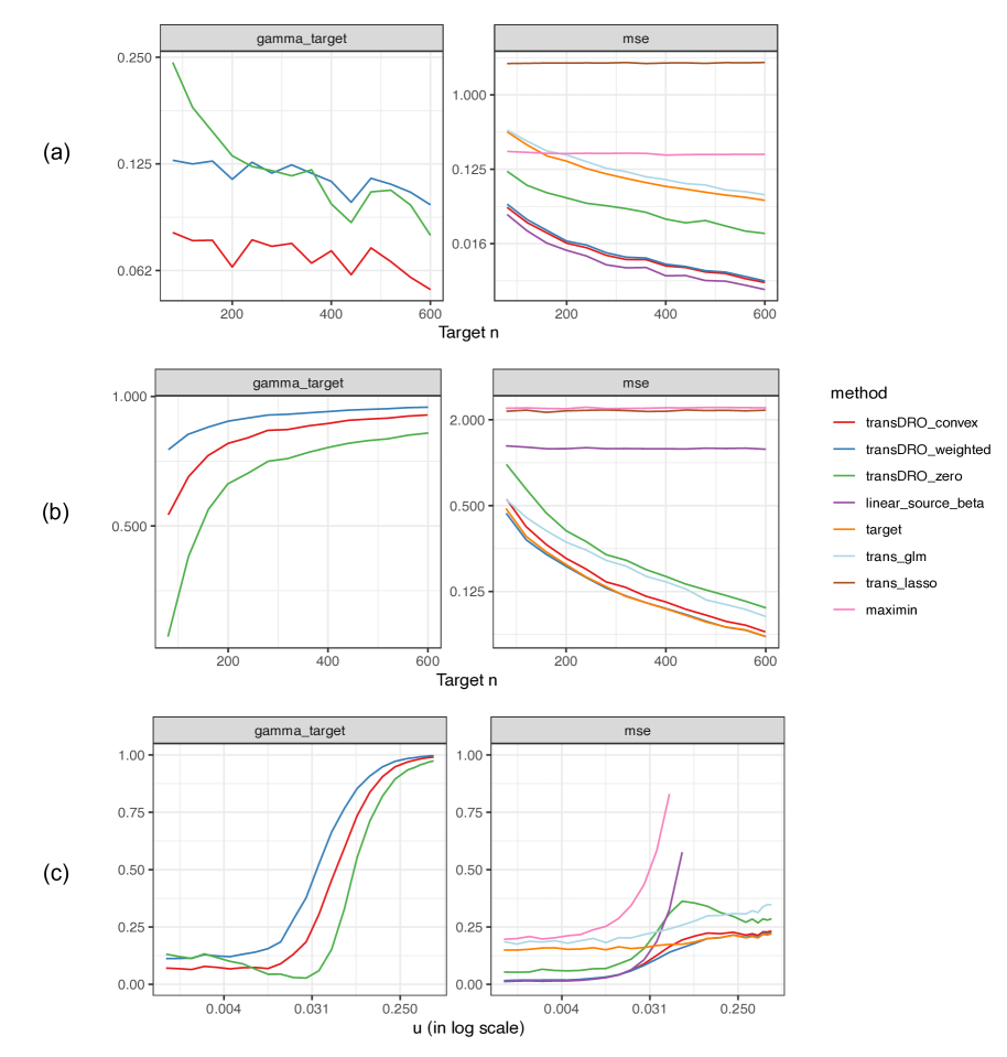
Figure 1: Weights assigned to the target site (i.e., $\widehat{\gamma}_{0}$) and estimation mse for (a) simulation setting 1.1 (fix $u=0.005$ and change $n$), (b) 1.2 (fix $u=0.1$ and change $n$), and (c) 1.3 (fix $n=200$ and change $u$). The x-axis in subplot (c) and all y-axis’s are in the log scale.

In setting 3, the validation model $\beta^{*}_{\mathrm{valid}}$ differs from the training target model $\beta^{*}$. We varied the size of the constraint set $\mathcal{S}(\tau)$ by changing $\tau$ from 0 to 1 and displayed the validation error in figure 2. As expected, a larger $\tau$ rendered a higher level of robustness and smaller prediction error for the TransDRO estimators, compared to their baseline. We also observed that TransDRO tends to assign less weight to the target especially when $\tau$ grows from 0 to a small value. Consistently, the prediction error drops in the same range of $\tau$ for TransDRO combined with the weighted and convex baseline, and then stabilizes to a low level. The declining rate for the target weight is the sharpest for the zero-based TransDRO, which also achieves the smallest mse when $\tau$ is small. However, less attention to the observed target does not equal a better prediction performance. Soon after $\tau$ exceeds 0.15, mse of zero-based TransDRO bounced up, though the target weight continues to drop. This may be due to the mismatch between the zero baseline and $\beta^{*}_{\mathrm{valid}}$. Recall the larger $\tau$ becomes, the larger $\mathcal{S}(\tau)$ is and the closer the TransDRO estimator gets to the zero baseline. Therefore, if there is no strong prior knowledge about the relationship between $\widehat{\beta}_{\mathrm{init}}$ and $\beta^{*}_{\mathrm{valid}}$, we suggest applying a relatively small but non-zero $\tau$ to keep both good model transferability and generalizability.

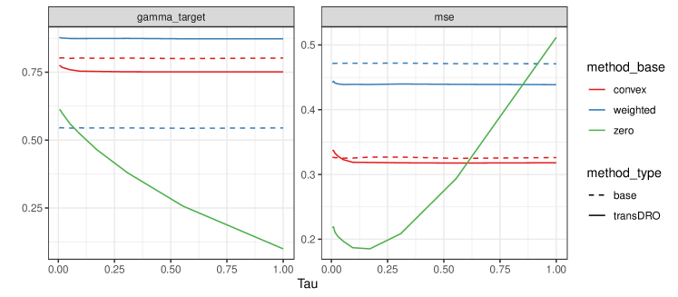
Figure 2: Weights assigned to the target site (i.e., $\widehat{\gamma}_{0}$) and estimation mse for simulation setting 3 (fix $n=200$ and change $\tau$).

4.3.2 High dimension

Under setting 4.1 with the existence of 5 adversarial sites among all 10 source sites, figure 3 shows the performance from different baselines as well as their corresponding TransDRO estimators. When we increase the number of variables with the adverse effect from 5 to 50, the average weight assigned to those adversarial sites decreases no matter which baselines the TransDRO estimator is equipped with. Yet, the decreasing rate differs. The weighted average baseline with weight varying from -1 to 1 (green dash line) acted most intensely when $p_{adv}$ increases to 50, where all the variables in the adversarial sites have the opposite sign of effects in contrast to the target site. Instead of assigning a zero weight, this baseline has the flexibility to set a negative weight and leverage the adversarial source information. As a consequence, TransDRO combined with such a baseline presented the smallest mse (green solid line). Interestingly, other than the $p_{adv}=50$ case, the weighted average baseline itself does not win over other baselines in terms of mse. It is the convex combination baseline that has the most robust performance. However, once integrated with TransDRO algorithm, the negative weights of the baseline assigned to the adversarial sites would guide the TransDRO effect in a benign way. Also, note that transGLM presented the best performance when $p_{adv}=5$ and all sources resemble the target site. As long as $p_{adv}$ increases to 10 or more, the superiority of transGLM disappears. We also tried to fix the number of variables with adverse effects and increase the number of adversarial sites from 2 to 8 in setting 4.2. The results have been shown in Appendix.

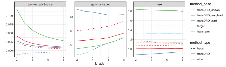
Figure 3: (Average) weights assigned to the target site (i.e., $\widehat{\gamma}_{0}$), to the adversarial sites (i.e., $\frac{1}{L_{adv}}\sum_{l=1}^{L_{adv}}\widehat{\gamma}^{(l)}$) and estimation mse for simulation setting 3.1 (fix $n=100$, $L_{adv}=5$ and change $p_{adv}$).

In setting 5, we fix the number of variables with non-zero effect as 100 and vary the $l_{1}$-level sparsity from 1 to 15. When nega_have=FALSE, there are 100 variables that have positive effects on the outcome among sources, but have null effects for the target outcome. Under this scenario, $s_{1}$ somehow takes a similar role as $u$ that measures the distance between the target and the best linear approximation $B\widetilde{\gamma}^{*}$. As a result, the left panel of figure 4 resembles the mse plot in figure 1 (c), where the mse of our TransDRO estimator takes the minimum of the target-only estimator and the source-combination estimator. Yet, unlike the poor performance in the low dimension case, TransDRO estimator with zero baseline shares close and sometimes even better prediction error compared to the convex combination baseline. Such advantage may be attributed to the design of a sparse $\beta^{*}$ under the high dimension case. Recall that we have shown in theorem 1 that the TransDRO effect is equivalent to the closest point to the baseline estimator within the constraint set. A zero baseline is expected to guide the TransDRO estimator to be more sparse, which is the desired property. Besides, mse from TransGLM also presents a different trend compared to simulation setting 1.3. Note that a smaller $s_{1}$ not only represents a diminishing gap between $\beta^{*}$ and $B\widetilde{\gamma}^{*}$, but also closer distance between $\beta^{*}$ and each $b^{(l)}$. Therefore, with a smaller $s_{1}$ (i.e., all sources are transferrable), both transGLM and our TransDRO estimator show superior performance. When $s_{1}$ grows, $\widehat{\mathcal{A}}_{h}$ shrinks gradually to only contain the target site and the final mse of transGLM also resembles TransDRO. However, the higher mse in the middle illustrates the insufficient usage of source data for the transGLM estimator when there are certain distance between source effects and the target effect.

When nega_have=TRUE, part of source effects of some variables are positive while the other sources have negative effects. The target still has most of the variables as null effects. In this scenario, simply taking the average of the source effects could recover the true $\beta^{*}$, as long as the sources with negative and positive effect are balanced. Therefore, we observe a better performance of the linear-source-combination estimator as well as our TransDRO estimator when $s_{1}$ increases. TransGLM also has a small mse, but such a superiority vanishes soon after $s_{1}$ exceeds a certain level.

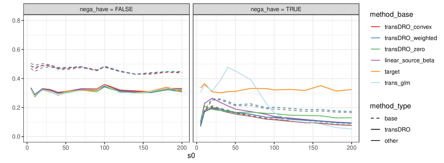
Figure 4: Estimation mse for simulation setting 4 (fix $s_{0}=100$, $n=100$, $p=307$ and change $s_{1}$).

5 Real data analysis

We validate our proposed TransDRO approach using the high-density lipoprotein (HDL) lab test data from UK Biobank (UKB) and Mass General Brigham (MGB) along with the genetic information. It is believed that the genetic underpinnings of mean lipoprotein diameter differ by race/ethnicity. Frazier-Wood et al. (2013) used genome-wide data to explicitly examine whether genetic variants associated with lipoprotein diameter in Caucasians also associate with those same lipoprotein diameters in non-Caucasian populations. They found that variation across the intronic region of the LIPC gene was suggestively associated with mean HDL diameters but only in Caucasians. In our real data analysis, we also focus on the 195 SNPs that were reported to be associated with mean HDL diameter in Caucasian. We will build a linear model on fasting mean HDL diameters using linear models, adjusted for age and sex. Yet, our target population becomes people with mixed and unknown ethnicity. In the UKB dataset, there is a small number of mixed-race groups between European and African and between Asian and European. By considering such multiracial people as the target group, it is reasonable to assume that the target model is equal/close to the mixture of source models built on the main racial groups. Similarly, model corresponding to people with missing race information are likely to come from a mixture of the existing single-race models, though there is less prior information about the the mixture proportion. Given the large source data (i.e., white, black, asian and others) and the proximity between the target group and the source races, we expect our TransDRO effect to efficiently transfer the genetic knowledge from the existing main races to the relatively rare target.

We first show the results for different UKB race groups. For each target race, we randomly sample 100 people as the training data set and another 100 people as the validation data set. When the target is specified as the white-asian mixed group, the left subplot on the first row of figure 5 and figure 6 illustrates the weights of different estimators assigned to the four main race sources and the target as well as the prediction mse. The performance of other estimators (e.g., different baselines) has been placed in the appendix. With whichever baseline, the Asian and European groups always received positive weights, which is consistent with the prior knowledge. The weighted combination baseline additionally assigned negative weights to the African and other groups, guiding the TransDRO effect to focus more on Asian and European sources. The guidance brought by the two baselines also led to a lower mse for the final TransDRO estimator. Due to the small number of target data, the target-only estimator suffers from a large mse. On the other hand, the estimator derived from the best linear combination of sources shared a similar mse as our TransDRO effects, indicating a close distance between $\beta^{*}$ and $B\widetilde{\gamma}^{*}$ as expected. When it comes to the White-Black mixed group, the right subplot on the first row of figure 5 and figure 6 depicts the superiority of our TransDRO models. By assigning a large proportion of attention to European and African groups while remaining a small weight to the limited target data, the TransDRO estimator achieves smaller mse than the minimum of target-only mse and source-combination mse. Due to the race heterogeneity, both the transGLM and transLasso model have a higher mse. Also, without any guidance from the target data, the maximin estimator assigned all weights to the European source group, which led to a relatively poor mse especially for the white-black target.

We also stratified the analysis by gender and show the TransDRO weights for white-asian UKB males and white-black females in the second row of figure 5 and figure 6. Still, the TransDRO estimator with the convex and the weighted baselines have the most stable performance with low mse. Also, even if the target population contains only one gender, we do observe a fair amount of weights coming from another gender (e.g., the existence of white females when predicting for white-asian males, and the existence of white males for the prediction among white-black females), which indicates shared effect across genders.

Figure 5: Weights of different estimators assigned to each race group. The top two rows use four race groups from UKB as sources, with the second row stratify data by gender. The left subplot on the third row utilizes MGB source data while the right one combine UKB and MGB together.

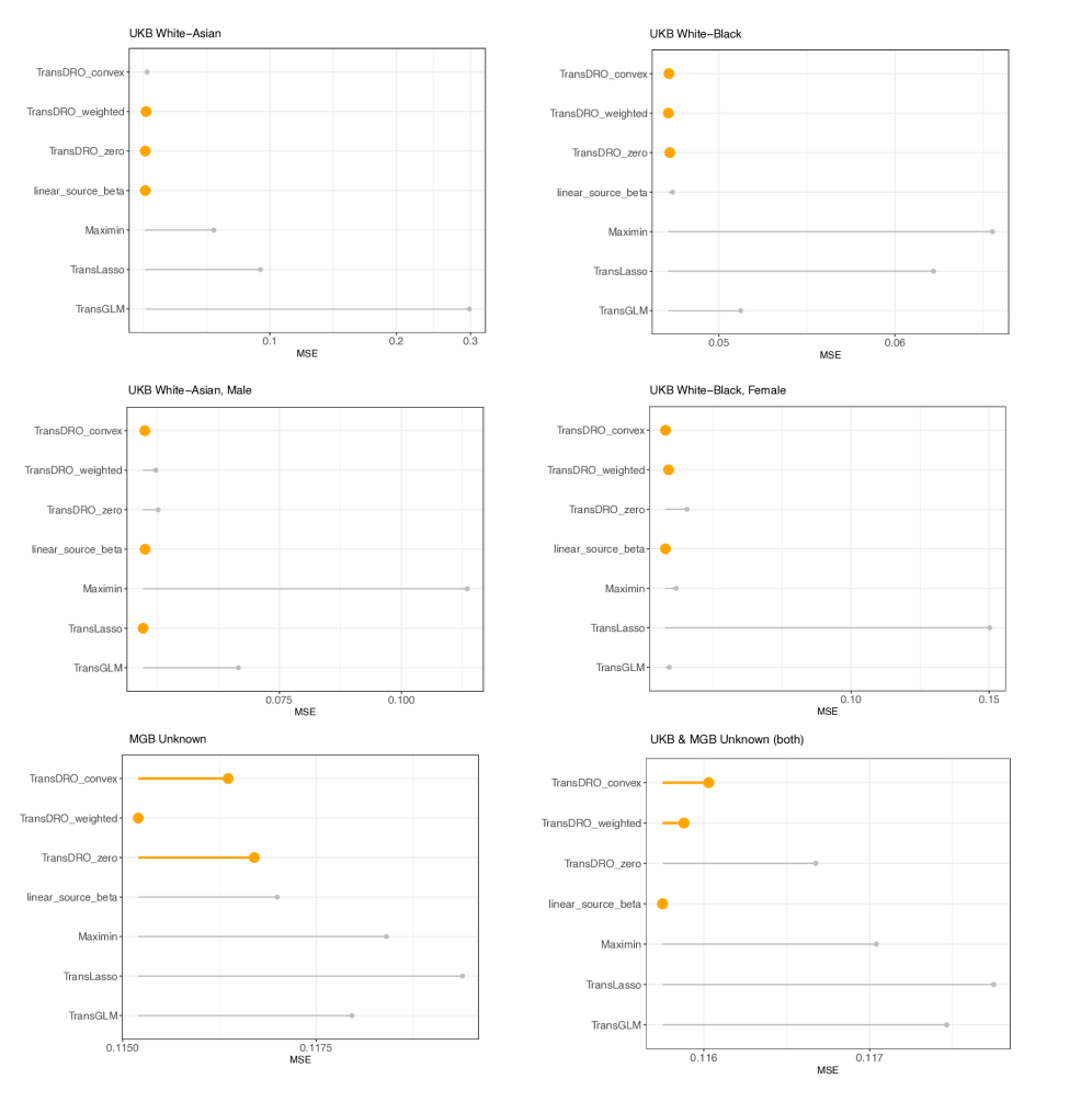
Figure 6: Estimation mse of different estimators. The top two rows use four race groups from UKB as sources, with the second row stratify data by gender. The left subplot on the third row utilizes MGB source data while the right one combine UKB and MGB together.

In terms of the MGB data, we focus on the unknown group. Among the target race, we sample 100 people as training target data and another 100 people as validation data set. The left subplot on the third row of figure 5 and figure 6 has shown that the unknown target might come from the mixture of white, asian and other race groups. Different baselines disagree with the contribution of the African group. The maximin and transLasso estimators claim the existence of black people, which are not included in the three version of TransDRO. Also, compared to TransDRO with weighted or convex baseline, zero-based TransDRO prefers to assign much more weights to the target site.

We also try to combine the unknown race group from the UKB and MGB together as the target and expand the source races to the four main racial groups across two sites (8 in total). The hope is to further leverage the shared knowledge in UKB and MGB, and decode the mixing component for the unknown group. The right subplot on the third row of figure 5 and figure 6 has shown the results where our TransDRO estimator with convex and weighted baselines achieved great performance with low mse again. Besides, the merging of unknown groups from two sources also leads to a higher weight assigned to the target, partly due to the increasing sample size.

References

- Desautels et al. [2017] T. Desautels, J. Calvert, J. Hoffman, Q. Mao, M. Jay, G. Fletcher, C. Barton, U. Chettipally, Y. Kerem, and R. Das. Using transfer learning for improved mortality prediction in a data-scarce hospital setting. Biomedical informatics insights, 9:1178222617712994, 2017.
- Frazier-Wood et al. [2013] A. C. Frazier-Wood, A. Manichaikul, S. Aslibekyan, I. B. Borecki, D. C. Goff, P. N. Hopkins, C.-Q. Lai, J. M. Ordovas, W. S. Post, S. S. Rich, et al. Genetic variants associated with vldl, ldl and hdl particle size differ with race/ethnicity. Human genetics, 132:405–413, 2013.
- Gligic et al. [2020] L. Gligic, A. Kormilitzin, P. Goldberg, and A. Nevado-Holgado. Named entity recognition in electronic health records using transfer learning bootstrapped neural networks. Neural Networks, 121:132–139, 2020.
- Guo [2023] Z. Guo. Statistical inference for maximin effects: Identifying stable associations across multiple studies. Journal of the American Statistical Association, pages 1–32, 2023.
- Hu et al. [2018] W. Hu, G. Niu, I. Sato, and M. Sugiyama. Does distributionally robust supervised learning give robust classifiers? In International Conference on Machine Learning, pages 2029–2037. PMLR, 2018.
- Laparra et al. [2021] E. Laparra, A. Mascio, S. Velupillai, and T. Miller. A review of recent work in transfer learning and domain adaptation for natural language processing of electronic health records. Yearbook of medical informatics, 30(01):239–244, 2021.
- Li et al. [2022] S. Li, T. T. Cai, and H. Li. Transfer learning for high-dimensional linear regression: Prediction, estimation and minimax optimality. Journal of the Royal Statistical Society Series B: Statistical Methodology, 84(1):149–173, 2022.