CaloShowerGAN, a Generative Adversarial Networks model for fast calorimeter shower simulation

Abstract

In particle physics, the demand for rapid and precise simulations is rising. The shift from traditional methods to machine learning-based approaches has led to significant advancements in simulating complex detector responses. CaloShowerGAN is a new approach for fast calorimeter simulation based on Generative Adversarial Network (GAN). We use Dataset 1 of the Fast Calorimeter Simulation Challenge 2022 to demonstrate the efficacy of the model to simulate calorimeter showers produced by photons and pions. The dataset is originated from the ATLAS experiment, and we anticipate that this approach can be seamlessly integrated into the ATLAS system. This development marks a significant improvement compared to the deployed GANs by ATLAS and could offer substantial enhancement to the current ATLAS fast simulations.

1 Introduction

Modern particle and nuclear physics programs require extensive, high-precision Monte Carlo (MC) simulations for modelling the response to particles that travel through the detector materials. This task is traditionally accomplished via a comprehensive detector simulation, utilising the Geant4 toolkit [1]. The most time-consuming part of the simulation process arises within the calorimeters, a sub-detector that measures energy deposits of particles. When the initial particle interacts with the dense material in the calorimeters, it generates secondary particles. This is a cascading process that can produce thousands of particles and form what is commonly known as a calorimeter shower. The large number of particles to be simulated is the origin of the time and resource-intensive nature of the Geant4 simulation. Overall, this aspect dominates the simulation time in collider experiments. As an example, in a typical event of a top and anti-top quark pair production simulated in the ATLAS experiment [2] at the Large Hadron Collider (LHC), the calorimeter shower simulation takes about $80\text{\,}\%$ of the total simulation time [3]. In the upcoming High Luminosity LHC program, the increased data volumes are expected to surpass the available computing capabilities for producing the necessary amount of MC events used in physics analyses [4, 5]. To uphold the consistent MC-to-data ratio, it becomes essential to substitute the calorimeter simulation, with a quicker alternative. This requirement has encouraged the creation of fast and high-fidelity calorimeter simulation techniques.

Numerous endeavours have been undertaken to expedite the simulation of calorimeter response while upholding satisfactory physics accuracy. The FastCaloSim method [6, 7], developed within the ATLAS Collaboration, is an example of such attempts. It involves the formulation of parameterised responses for the calorimeter, tailored to specific types of incoming particles. By employing this parametrisation, it accelerates the speed of simulating an event by approximately a factor of ten, effectively bypassing the intricate shower development process carried out by Geant4. In a novel line of research, including studies in Refs. [8, 9, 10, 11, 12, 13, 14, 15, 16, 17, 18, 19, 20, 21, 22, 23, 24, 25, 26], machine learning approaches using cutting-edge generative techniques are proposed for generating the calorimeter response. In the recently developed AtlFast3 [27], the new generation of high-accuracy fast simulation in ATLAS, a combination of parametric and machine learning approaches (FastCaloSimV2 [27] and FastCaloGAN [20], respectively) is adopted to achieve optimal performance in terms of both speed and simulation accuracy across the detector’s full phase space.

In this context, the research community organised the Fast Calorimeter Simulation Challenge 2022 [28], hereinafter referred to as CaloChallenge. CaloChallenge is a newly introduced community challenge that aims at motivating the development of generative algorithms to address the calorimeter simulation challenge. Standardised datasets and tools to facilitate training and validating processes are provided too.

In this paper, we present a fast calorimeter simulation model using Generative Adversarial Networks (GANs) technique, named CaloShowerGAN, with a focus on utilising the first dataset provided by the CaloChallenge. Other models that participated in the CaloChallenge using this dataset, at the time of writing this paper, are documented in Refs. [18, 26].

The paper is organised as follows. Section 2 briefly describes the datasets used in this study provided by the challenge. The CaloShowerGAN model description, hyper-parameter optimisation, and training procedure are detailed in Section 3. Further optimisations are described in Section 4. The results and performances of CaloShowerGAN are presented in Section 5. Future research directions are presented in Section 6 followed by conclusions in Section 7.

2 Input datasets

The first dataset provided by the challenge is part of the ATLAS open dataset [29] used in AtlFast3 [27]. It comprises two distinct subsets representing different particle types, the photon and the charged pion sets. These data are generated by ATLAS using Geant4 with the official ATLAS detector geometry, ensuring that they accurately represent genuine electromagnetic and hadronic showers. Each subset consists of 15 samples with different incident momenta generated at the calorimeter surface, followed by noise-free simulation to facilitate the training of accurate showers. The incident momentum of the samples ranges from $256\text{\,}\mathrm{MeV}$ to $4\text{\,}\mathrm{TeV}$, increasing in powers of two. In the range from $256\text{\,}\mathrm{MeV}$ to $256\text{\,}\mathrm{GeV}$, 10000 events are simulated at each energy value, while for higher momenta, the statistical count decreases. An overview of these statistics is depicted in Figure 1.

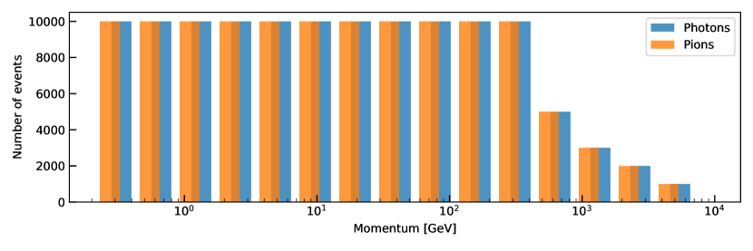
Figure 1: Statistics of Dataset 1 in the CaloChallenge under each incident momentum.

All events are generated within the $|\eta|$ range of $[0.20,0.25]$, aligning with the ATLAS’ chosen strategy for parameterising the complete detector response. Further insights into the reasoning behind this strategy and comprehensive sample details can be found in Ref. [27]. In each event, the spatially distributed energy deposits simulated by Geant4 are referred to as “hits”. These hits are initially defined in Cartesian coordinates and subsequently transformed into cylindrical coordinates ($r$, $\alpha$, layer) along the particle’s flying direction. Here, $r$ is the distance of the hit from the intersection point between the extrapolation of the generated particle and the layer, while $\alpha$ denotes the polar angle in cylindrical coordinates. The coordinate “layer” corresponds to the physical instrumented layer within the ATLAS calorimeter, indicating the extent of particle propagation from the origin of the detector. The first four layers, numbered 0–3 according to the ATLAS naming scheme, are electromagnetic calorimeters dedicated to the measurement of electromagnetic showers while the following layers, denoted as 12, 13, and 14, are part of hadronic calorimeters used to measure hadronic showers. Subsequently, the hits within each layer are aggregated into volumes referred to as “voxels”, with the energy within a voxel being the cumulative sum of the energies contributed by all the associated hits. The number of voxels in each layer for the two subsets is summarised in Table 1. The energy deposits in voxels are used as the input for the CaloShowerGAN and are the information that the generative model aims to reproduce.

Table 1: Configuration of voxels in the training dataset in each layer. Note that photons do not penetrate significantly in the hadronic calorimeter; therefore, they comprise fewer layers. $N_{r}$ and $N_{\alpha}$ are the number of bins in the $r$ and $\alpha$ directions, respectively. $N_{\text{voxel}}$ is the number of voxels.

Particle	Layer	$N_{r}$	$N_{\alpha}$	$N_{\text{voxel}}$
$\gamma$	$0$	$8$	$1$	$8$
	$1$	$16$	$10$	$160$
	$2$	$19$	$10$	$190$
	$3$	$5$	$1$	$5$
	$12$	$5$	$1$	$5$
Total				$368$
$\pi$	$0$	$8$	$1$	$8$
	$1$	$10$	$10$	$100$
	$2$	$10$	$10$	$100$
	$3$	$5$	$1$	$5$
	$12$	$15$	$10$	$150$
	$13$	$16$	$10$	$160$
	$14$	$10$	$1$	$10$
Total				$533$

3 Model and hyperparameters

CaloShowerGAN is designed to have a similar structure to FastCaloGAN available in Ref. [30] so that it can be easily integrated by the ATLAS collaboration. At the same time, the tool’s foundation diverges notably from FastCaloGAN, leading to superior performance. This advancement is realised through revisions in training data pre-processing and adjustments in model architecture and hyperparameters. Several of these enhancements are underpinned by significant expertise in understanding the intricate details of how showers interact within the calorimeter.

3.1 CaloShowerGAN

CaloShowerGAN is constructed on the foundation of the Conditional Wasserstein GAN algorithm [31, 32], which has been established for delivering good performance and training stability. To effectively simulate calorimeter showers across a broad range of incident momenta spanning multiple orders of magnitude, CaloShowerGAN is conditioned on the true kinetic energy of the incoming particle. This variable is preferred because the characteristics of the shower are directly proportional to the logarithm of the kinetic energy of the particle rather than the momentum. The architecture of CaloShowerGAN employed in this study is depicted in Figure 2. The generator comprises three hidden layers and one output layer. Each layer incorporates a dense layer, followed by batch normalisation [33] and an activation operation. The generator receives a noise vector randomly sampled from a high-dimensional normal distribution, where each dimension has a mean and standard deviation of $0.5$. The condition label of the generated event is simultaneously fed as input.

The output of the generator aligns with the number of voxels and is subsequently input into the discriminator as “fake” events, along with the concatenated condition label. The “real” events are taken from the dataset outlined in Section 2, joined with their actual condition labels. The discriminator encompasses three dense layers with a ReLU activation function. No batch normalisation operation is employed, as it is found not to enhance performance. Instead, spectral normalisation [34] is adopted to stabilise the training.

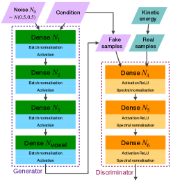
Figure 2: Schematic view of the CaloShowerGAN architecture. The generator comprises three hidden layers with node counts of $N_{1}$, $N_{2}$, and $N_{3}$, respectively, along with an output layer sized to match the number of voxels. Each layer consists of a dense layer, followed by a batch normalisation operation and an activation operation. A 1-dimensional condition representing kinetic energy is used, alongside a 50-dimensional latent vector randomly sampled from a normal distribution with both mean and standard deviation of 0.5. The generator’s output, concatenated with the condition label, is input to the discriminator. The discriminator comprises three dense layers with a ReLU activation function. Spectral normalisation operation is used within the discriminator to stabilise the training. The generator’s activation function and both networks’ sizes vary between photon and pion GANs.

3.2 Data preprocessing

The input data comprises energy deposits in voxels, measured in megaelectronvolts (MeV) and structured in an $n\times m$ matrix. Here $n$ represents the number of voxels, and $m$ denotes the number of events. Furthermore, the energy of each voxel is normalised based on the kinetic energy of the particle. This is similar to what is done in FastCaloGAN. This normalisation procedure allows to standardise all values within the input vector to a similar order of magnitude for all input momenta, effectively eliminating the significant difference between the momenta of the samples. In this way, the GAN can focus on reproducing the shape of the showers rather than its absolute value. The condition label is transformed to a normalised range of $[0,1]$ using the following equation:

$$\hat{E}=\frac{\log{\frac{E_{\text{kin}}}{E_{\text{min}}}}}{\log{\frac{E_{\text{max}}}{E_{\text{min}}}}}.$$ (1)

Here $E_{\text{min}}$ ($E_{\text{max}}$) is the minimum (maximum) kinetic energy of the incoming particle in the training data. It has been observed that this scheme yields a notable improvement over an alternative method employed in FastCaloGAN.

3.3 Training

The training process for CaloShowerGAN involves independent training on distinct particle samples to maximise performance. Each training employs a batch size of $1024$ and runs for a total of $10^{6}$ iterations. Model checkpoints are created at intervals of $10^{3}$ iterations. Due to the adversarial nature of GAN training, the final iteration does not necessarily yield the best outcome. To address this, the approach of saving multiple iterations is adopted. This approach has two-fold benefits: it enables swift training without evaluation during the process, and it offers flexibility in assessing the optimal iteration using diverse strategies, obviating the need for GAN re-training.

Inspired by the methodology used in FastCaloGAN, the assessment metric is the total energy associated with each of the 15 incident momentum points. The $\chi^{2}$ value for each GAN model is computed between the binned distributions of the Geant4 sample and generated sample by the model and then normalised by the number of degrees of freedom used in each distribution ($\chi^{2}$/NDF). The model that gives the lowest $\chi^{2}$/NDF among the saved iterations is deemed the best. This selection process has proven to be a reliable metric for gauging the overall quality of a shower. It is found that the shape of the generated showers consistently improves in models with lower $\chi^{2}$/NDF values.

The GAN architecture comprises various hyperparameters that are amenable to optimisation. Beginning with the values employed in FastCaloGAN, the optimisation process encompasses the refinement of several parameters, including the learning rate and momentum for both the generator and discriminator optimisers, the batch size, the discriminator-to-generator (D/G) ratio, the $\lambda$ that controls the penalty contribution in the Wasserstein GAN, and the choice of activation functions. The D/G ratio, quantifying the number of times the discriminator is trained relative to a single training pass of the generator in each iteration, is found to play a pivotal role. Generator and discriminator sizes, ranging from one-quarter of the determined size to as much as four times the size, are explored. Optimisation algorithms are also investigated beyond the commonly used Adam [35] optimiser including RAdam [36] coupled with LookAhead [37], as well as AdamW [38]. It was observed that these alternative optimisers yielded sub-optimal performance when compared to Adam.

Eventually, the Adam optimiser is selected for both the generator and discriminator, utilising a learning rate of $10^{-4}$ and a momentum value of $\beta_{1}=0.5$. These values are used for both pion and photon GANs.

Hyper-parameters for Photon CaloShowerGAN. The utilisation of the Swish [39] activation function in the photon CaloShowerGAN yields superior performance compared to more common choices like ReLU [40]. While Swish activation can potentially introduce training instability, this drawback appears to be mitigated when coupled with the Glorot Normal [41] initialisation method for the generator neuron weights. Conversely, the ReLU activation, employed in conjunction with the He Uniform [42] initialisation, finds its place in the discriminator. Notably, a higher D/G ratio proves advantageous in strengthening the discriminator’s potency against the generator, particularly when using the Swish activation function.

The size of the networks is chosen as follows. The latent dimension is set to $100$, allowing for intricate data representation. The width of the generator layers is increasing in the three hidden layers, from $100$, $200$, to $400$. This scale is twice that of the generators seen in the FastCaloGANs, offering a substantial leap in capacity and potential. The discriminator size of all three hidden layers is fixed to the number of voxels, i.e. $368$. The value of $\lambda$ is chosen to be $3$.

Hyper-parameters for Pion CaloShowerGAN. The pion CaloShowerGAN employs the ReLU activation due to its superior performance compared to Swish. Both the latent dimension and the size of the generator layers have been carefully optimised. The latent dimension is chosen to be $200$. The width of the generator layers is tailored to be $200$, $400$, and $800$, respectively. Note the dimensions are larger than the photon CaloShowerGAN to account for the larger voxel count employed for pions, along with the intrinsically higher complexity and variety of hadronic showers. Larger networks are tested but fail to yield substantial gain and significantly extend the training time, hence they are not considered. The optimal discriminator size mirrors that of the generator, although it assumes a distinct configuration from the one employed for photons. The discriminator sizes sequentially progress from $533$ voxels in the input layer to $800$, $400$, and $200$ in subsequent layers. Maintaining a low D/G ratio and a relatively higher value of $\lambda$ are found to be optimal. The introduction of batch normalisation does not emerge as a crucial factor in improving the performance, but it is applied to be consistent with the photon CaloShowerGAN.

An overview of the hyperparameters used in the photon and pion CaloShowerGAN is shown in Table 2.

Table 2: Determined hyperparameter values for the photon and pion GANs.

Hyperparameter	Photon	Pion
Latent space size	$100$	$200$
Generator size ($N_{1},N_{2},N_{3}$)	$100$, $200$, $400$	$200$, $400$, $800$
Discriminator size ($N_{4}$, $N_{5}$, $N_{6}$)	$368$, $368$, $368$	$800$, $400$, $200$
Generator optimiser	Adam	Adam
Learning rate	$1\text{\times}{10}^{-4}$	$1\text{\times}{10}^{-4}$
$\beta_{1}$	$0.5$	$0.5$
$\beta_{2}$	$0.999$	$0.999$
Discriminator optimiser	Adam	Adam
Learning rate	$1\text{\times}{10}^{-4}$	$1\text{\times}{10}^{-4}$
$\beta_{1}$	$0.5$	$0.5$
$\beta_{2}$	$0.999$	$0.999$
Batch size	$1024$	$1024$
D/G ratio	$8$	$5$
$\lambda$	$3$	$20$
Activation (generator)	Swish	ReLU
Activation (discriminator)	ReLU	ReLU
Neuron weight initialisation (generator)	Glorot Normal	He Uniform
Neuron weight initialisation (discriminator)	He Uniform	He Uniform
Trainable parameters (generator, discriminator)	$261$k, $408$k	$871$k, $829$k

3.4 Intermediate results after hyperparameter optimisation

The performance of the selected CaloShowerGAN is presented in Figures 3–4 where the distribution of the total energy for generated events and the input Geant4 sample are compared for all momentum points for photons and pions respectively. Each pad contains the $\chi^{2}_{i}/\text{NDF}_{i}$ for the specific momentum $i$ while the total $\chi^{2}$/NDF is displayed at bottom right, calculated as $\Sigma_{i}{\chi^{2}}/\Sigma_{i}\text{NDF}$.

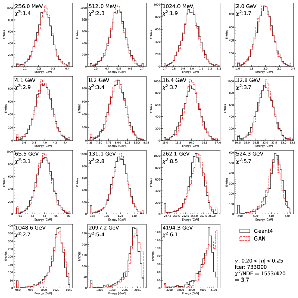
Figure 3: Photon CaloShowerGAN. The calorimeter response for the Geant4 simulation (solid black line) compared to CaloShowerGAN (dashed red line) for photons in the full momentum range. The $\chi^{2}$ values in each sub-panel are calculated from the distributions in that incident energy and the final $\chi^{2}$ is calculated from the concatenation of the histograms in all energies.

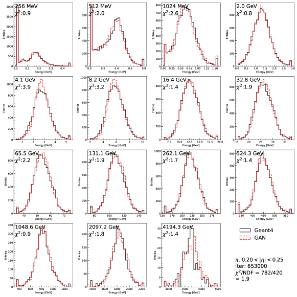
Figure 4: Pion CaloShowerGAN. The calorimeter response for the Geant4 simulation (solid black line) compared to CaloShowerGAN (dashed red line) for pions in the full momentum range. The $\chi^{2}$ values in each sub-panel are calculated from the distributions in that incident energy and the final $\chi^{2}$ is calculated from the concatenation of the histograms in all energies.

On the whole, CaloShowerGAN yields notably improved results in comparison to the similar distributions presented in FastCaloGAN [27]. The results attained for pions exhibit remarkable agreement across all momentum points, yielding a total $\chi^{2}$/NDF value of 1.9. Only a few distributions show small deviations from the Geant4 distributions, and notably, there is no pronounced distinction in modelling either high or low momenta. The level of agreement achieved for photons GAN falls short, manifesting as a total $\chi^{2}$/NDF value of 3.7, nearly twice that achieved for pions. There is a clear trend in the values of the individual $\chi^{2}$/NDF which are worse for the higher momenta. The agreement worsened above 262 GeV with a visible shift in the generated distributions. These are likely caused by the difficulty in reproducing the asymmetric distribution of the total energy. These pitfalls motivates the further development below.

CaloShowerGAN represent a significant improvement not only in terms of physics performance but also in training speed when compared to FastCaloGAN. The optimised CaloShowerGAN requires approximately 6 hours while FastCaloGAN required over 16 hours on a GPU card with a similar computational setup.

4 Further optimisation of CaloShowerGAN

4.1 Momentum split for photon GAN

As depicted in Figure 3, the performance of the photon CaloShowerGAN reveals a dependence on the photon momentum, characterising three distinct momentum regions. These regions are distinct by specific features of the electromagnetic showers within the ATLAS calorimeter, which can pose challenges to the training process of CaloShowerGAN:

1. In the low-momentum region, i.e. for momenta up to 4 GeV, particles deposit almost all their energy in the initial two layers of the calorimeter. In the remaining layers, the voxels have minimal or negligible energy deposits, accompanied by significant event-to-event fluctuations. These fluctuations, absent in higher-momentum regions where all voxels are populated, can potentially confuse CaloShowerGAN during the learning process.

2. In the medium-momentum range between 8 GeV and 262 GeV, the energy is deposited predominantly in layer 2 as this is the layer with the largest amount of material. This presents a contrasting scenario compared to the lower momentum range. Here, the first two layers, while containing some energy, contribute insignificantly to the overall energy deposit.

3. Lastly, the samples with a momentum above 262 GeV are characterised by an asymmetric response in the total energy. This asymmetry is attributable to the shower extending beyond the confines of the voxel volume and is compounded by non-linearities in the calorimeter’s response, which are more significant at higher energy levels.

The mixture of events from these three distinct momentum groups during training introduces complexity to the learning process. Thus, the generation of photon showers in CaloShowerGAN is separated in three GANs, initialised with the previously outlined parameters, within the energy intervals of [256 MeV, 4 GeV], [4 GeV, 262 GeV], and [262 GeV, 4 TeV]. These GANs share a common momentum point to allow seamless interpolation across all momentum points.

An additional limited HP scan is conducted to fine-tune the three GANs. The outcomes affirm that the majority of the employed hyperparameters are indeed optimal for all three GANs, requiring only minor adjustments to achieve improved performance. In the low-momentum range, the ReLU activation function takes over Swish, while the He Uniform initializer replaces Gloroth. For the two GANs trained in the higher momentum ranges, superior results are achieved using a downscaled generator network along with a latent space size reduced by half compared to the single GAN configuration.

The adoption of this approach yields a clear enhancement, evidenced by the lowered $\chi^{2}$/NDF values for each individual GAN as compared to the single GAN’s value of 3.7. In the low-momentum GAN, $\chi^{2}$/NDF values across all momentum points are improved, with the exception of the 4 GeV sample where a visible distribution shift contributes to a raised $\chi^{2}$/NDF. In the medium-momentum range, all momentum points exhibit a reduced $\chi^{2}$/NDF compared to the corresponding values obtained using the single GAN. However, the most substantial improvement is observed within the high-momentum range, where the previously observed disparity between generated events and input samples is effectively mitigated. The $\chi^{2}$/NDF results are summarised in Table 3 where a further result is derived using two GANs. While this alternative offers decreased precision compared to the three-GAN approach, it might still be valuable to consider by an experiment as it demands shorter training times and less memory during detector simulation when conducting inference.

Table 3: Performance of the photon CaloShowerGAN when splitting in different momentum ranges. The “sum”-med $\chi^{2}$ and NDF are the sum of these values for the GANs considered.

Name	momentum range	$\chi^{2}$	NDF	$\chi^{2}/\text{NDF}$
Single GAN	[$256\text{\,}\mathrm{MeV}$, $4\text{\,}\mathrm{TeV}$]	$1553$	$420$	$3.7$
	[$256\text{\,}\mathrm{MeV}$, $4\text{\,}\mathrm{GeV}$]	$360$	$140$	$2.6$
	[$4\text{\,}\mathrm{GeV}$, $4\text{\,}\mathrm{TeV}$]	$1042$	$308$	$3.4$
Two GANs	Sum	$1402$	$448$	$3.1$
	[$256\text{\,}\mathrm{MeV}$, $4\text{\,}\mathrm{GeV}$]	$360$	$140$	$2.6$
	[$4\text{\,}\mathrm{GeV}$, $262\text{\,}\mathrm{GeV}$]	$528$	$196$	$2.7$
	[$262\text{\,}\mathrm{GeV}$, $4\text{\,}\mathrm{TeV}$]	$299$	$140$	$2.1$
Three GANs	Sum	$1187$	$476$	$2.5$

This approach is not applicable to pions, primarily due to the inherent characteristics of hadronic showers. Even at lower energies, hadronic showers tend to distribute some energy across all layers. Consequently, splitting pion training into multiple GANs results in a compromised overall performance and is therefore not recommended.

4.2 Layer-energy normalisation

Despite the enhanced results stemming from the 3-GAN approach in the photon GAN, the overall performance still falls short of that demonstrated by CaloFlow [18], which currently stands as the leading model. At the time of writing, CaloFlow attains a remarkable $\chi^{2}$/NDF value of 1.17 for photons and 1.32 for pions. In pursuit of further enhancements, various strategies were explored. The most significant improvement is achieved by adopting a different normalisation strategy used in Ref. [43] for the input data used during CaloShowerGAN training. Additional studies were performed and some of them are detailed in Section 6.

The normalisation detailed in Section 3.2 lacks constraints on pivotal physics quantities, such as layer-specific energy and total energy. While this information is inherently present in the data, not explicitly providing it to the GANs makes the learning process more challenging compared to the potential ease that clear constraints are provided as part of the inputs. This information can be encoded using the following normalisation procedure: Firstly, the voxel energy is normalised with respect to the total energy in the corresponding layer. Subsequently, the energy in each layer is normalised to the total energy in the shower, resulting in 5 (7) new input dimensions for the photon (pion) GANs. Another input is incorporated, representing the ratio between the total shower energy and the kinetic energy of the incident particle.

Adopting this normalisation strategy requires modifications to the final generator layer. The output nodes are grouped based on the voxel count in each layer, and a SoftMax activation function is applied to each group to enforce layer-wise normalisation. Similarly, 5 (7) nodes, corresponding to the total deposits of photons (pions) in each layer, are grouped, employing another SoftMax activation. The last node, linked to the normalised total deposits in the entire calorimeter, employs a ReLU activation function. In the discriminator, only the input layer size is altered to accommodate the additional values. In the case of pions, it is worth noting that longer training times can be particularly beneficial; actually, pions with lower momenta continue to show significant learning improvements even after 1 million iterations. Therefore, for pions, the number of iterations used for the training is extended to 2 million, therefore doubling the training time to 12 hours. As a result, the cumulative training time for CaloShowerGAN is approximately 30 hours, which remains less than the 32 hours used for FastCaloGAN.

5 Performance of CaloShowerGAN

5.1 Total energy

The results of CaloShowerGAN with the layer-energy normalisation are depicted in Figures 5–6. By employing layer-energy normalisation, a substantial improvement in $\chi^{2}$/NDF is observed. In particular, the performance achieved by CaloShowerGAN on the pion dataset is significant and it reaches a comparable performance to that of CaloFlow [18] in terms of the $\chi^{2}$/NDF metric. Notably, it is essential to recognise that there exists a slight disparity in the definition of $\chi^{2}$/NDF between the two studies. While in this study the actual number of degrees of freedom (NDF) is adopted by excluding empty bins, the CaloFlow incorporates the total number of bins in the normalisation. Considering the proximity of the sum of all $\chi^{2}$ values, we conclude that the two models exhibit closely comparable performance.

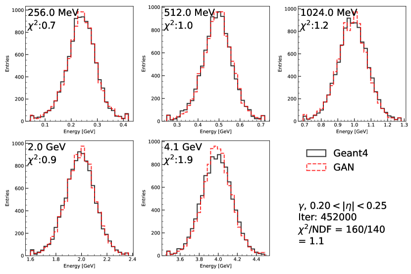
(a) low-momentum, 256 MeV–4 GeV

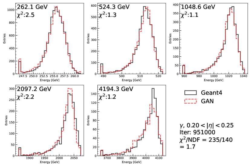
(b) high-momentum, 262 GeV–4 TeV

(c) Midium-energy, 4 GeV–262 GeV

Figure 5: Photon CaloShowerGAN with layer-energy normalisation. The calorimeter response for the Geant4 simulation (solid black line) compared to CaloShowerGAN (dashed red line) for photons samples in the three momentum ranges using the layer-energy normalisation. The $\chi^{2}$ values in each sub-panel are calculated from the distributions in that incident energy and the final $\chi^{2}$ is calculated from the concatenation of the histograms in all energies.

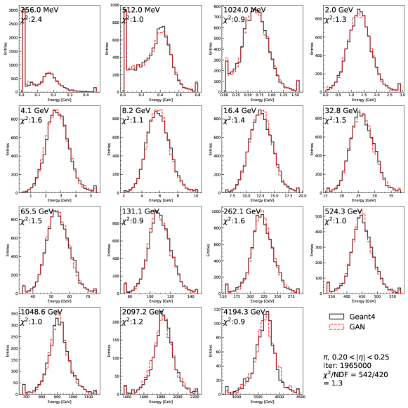
Figure 6: Pion CaloShowerGAN, with layer-energy normalisation. The calorimeter response for the Geant4 simulation (solid black line) compared to CaloShowerGAN (dashed red line) for pions in the full momentum range using the layer-energy normalisation. The $\chi^{2}$ values in each sub-panel are calculated from the distributions in that incident energy and the final $\chi^{2}$ is calculated from the concatenation of the histograms in all energies.

Detailed comparisons using more complex metrics, such as a classifier, are the objective of the CaloChallenge, where both models are actively participating. Therefore, we defer further quantitative comparisons beyond the scope of the $\chi^{2}$/NDF metric to the CaloChallenge, where these considerations are appropriately addressed in a consistent and fair way for all models.

The results obtained from the 3 GANs used to simulate the full momentum range of the photon dataset are summarised in Table 4. While CaloShowerGAN does not quite match the performance level of CaloFlow, it still attains a commendable accuracy. This achievement holds substantial promise for enhancing the efficiency of GANs employed by ATLAS.

Table 4: CaloShowerGAN, with layer-energy normalisation. The “sum”-med $\chi^{2}$ and NDF are the sum of these values for the GANs considered.

Name	momentum range	$\chi^{2}$	NDF	$\chi^{2}/\text{NDF}$
Photon single GAN	$256\text{\,}\mathrm{MeV}$–$4\text{\,}\mathrm{TeV}$	$1131$	$420$	$2.7$
	$256\text{\,}\mathrm{MeV}$-$4\text{\,}\mathrm{GeV}$	$160$	$140$	$1.14$
	$4\text{\,}\mathrm{GeV}$–$4\text{\,}\mathrm{TeV}$	$703$	$308$	$2.3$
Photon two GANs	Sum	$863$	$448$	$1.9$
	[$256\text{\,}\mathrm{MeV}$, $4\text{\,}\mathrm{GeV}$]	$160$	$140$	$1.1$
	[$4\text{\,}\mathrm{GeV}$, $262\text{\,}\mathrm{GeV}$]	$450$	$196$	$2.3$
	[$262\text{\,}\mathrm{GeV}$, $4\text{\,}\mathrm{TeV}$]	$235$	$140$	$1.7$
Photon three GANs	Sum	$845$	$476$	$1.8$
Pion GAN 1M	[$256\text{\,}\mathrm{MeV}$, $4\text{\,}\mathrm{TeV}$]	$628$	$420$	$1.5$
Pion GAN 2M	[$256\text{\,}\mathrm{MeV}$, $4\text{\,}\mathrm{TeV}$]	$542$	$420$	$1.3$

5.2 Stability of the training

The training of a GAN, being an adversarial game between the two networks, is not a well-defined minimisation problem. In general, a longer training should produce a better result; however, as stated previously, the optimal GAN may not always come from the final iteration of the training due to the adversarial nature of the process. Therefore, the behaviour of $\chi^{2}$/NDF over the saved iterations is examined. The progression of $\chi^{2}$/NDF throughout iterations is visually represented in Figure 7 and Figure 8 for photons and pions, respectively. Evidently, the $\chi^{2}$/NDF values for both individual energies and the aggregate exhibit a decreasing trend as a function of the iteration and reach a relatively stable value toward the end of the training, indicating the model is progressively improving during training. It is interesting to observe that the best overall model, i.e. the one that produces the best total $\chi^{2}$/NDF, may not coincide with the optimal iteration for a specific momentum. The present selection methodology procedure is a balance between performance across all momentum points, representing a compromise solution. In general, the final selection is driven by momentum points that are relatively less accurately modelled, as these contribute the most to the overall total $\chi^{2}$/NDF.

In the case of pions, a notable distinction emerges in the progression of $\chi^{2}$/NDF across various momentum points. Higher momentum points tend to converge more rapidly towards a stable solution, while lower momentum points exhibit a relatively slower convergence in $\chi^{2}$/NDF. The longer training used for the pions assures that a good convergence is achieved for all energies.

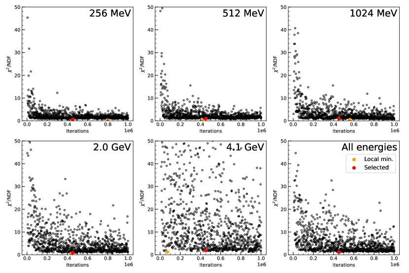
(a) low-momentum, 256 MeV–4 GeV

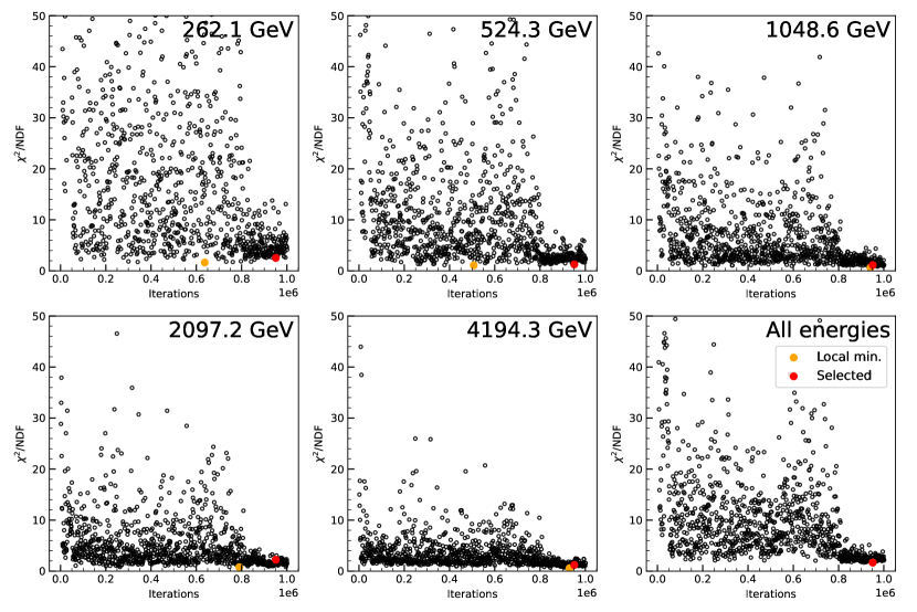
(b) high-momentum, 262 GeV–4 TeV

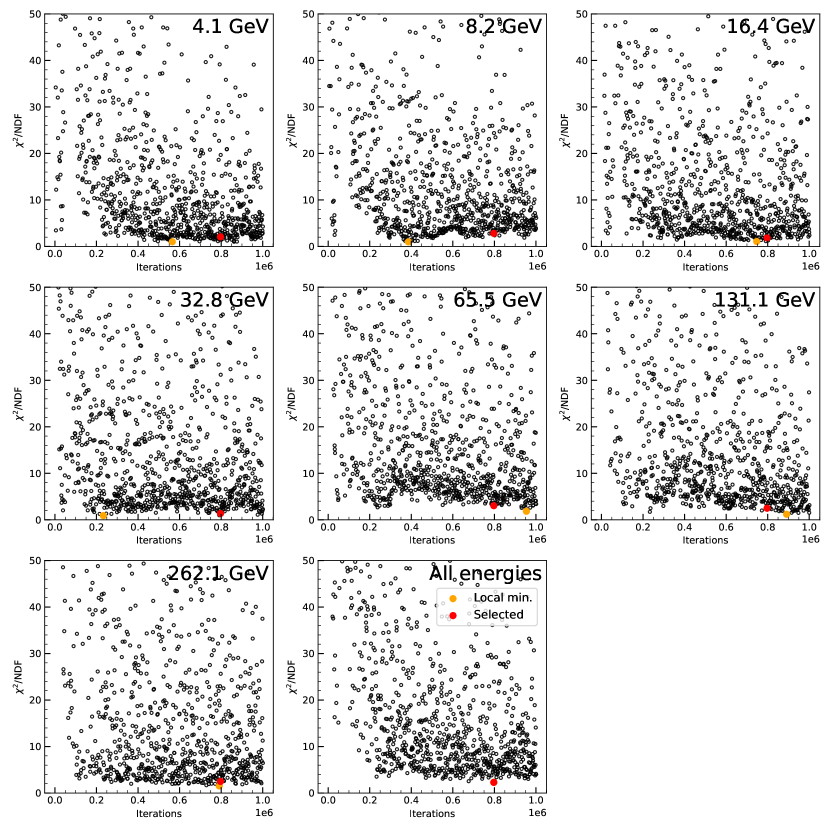
(c) Midium-energy, 4 GeV–262 GeV

Figure 7: Photon CaloShowerGAN, with layer-energy normalisation. Evolution of the individual and total $\chi^{2}$ as a function of iteration in photons. The first $N-1$ panels show the individual $\chi^{2}$/NDF for a momentum energy and the last panel shows the total $\chi^{2}$/NDF. The selected iteration is indicated in red dot while the orange dots in the individual cases indicate the lowest $\chi^{2}$/NDF when only considering that momentum.

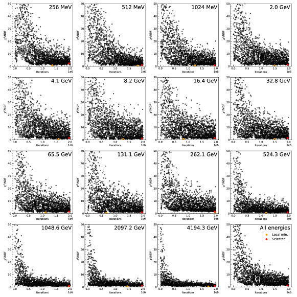
Figure 8: Pion CaloShowerGAN, with layer-energy normalisation. Evolution of the individual and total $\chi^{2}$ as a function of iteration in pions. The first $N-1$ panels show the individual $\chi^{2}$/NDF for a momentum energy and the last panel shows the total $\chi^{2}$/NDF. The selected iteration is indicated in red dot while the orange dots in the individual cases indicate the lowest $\chi^{2}$/NDF when only considering that momentum.

5.3 Energy per layer

While a satisfactory concordance in the total energy of showers might suggest success, it does not necessarily ensure the GANs’ ability to replicate the complex structure of these showers. To validate this point, the energy distributions across each calorimeter layer are shown in Figure 9 and Figure 10. Good agreement with the Geant4 samples is observed when samples of all incident momentum points are merged together. .

In the case of photons depicted in Figure 9, layer 0 poses a slight challenge for modelling, as the GANs slightly overshoot the intended energy deposits. It is important to highlight that this effect is relatively minor, considering the logarithmic scale of the plots. In fact, it affects less than 1% of the events. Moreover, the effect is limited for physics performance, as ATLAS electron and photon reconstructions primarily rely on layers 1 and 2.

For pions in Figure 10, a bimodal structure emerges in several layers for momenta below $1\text{\,}\mathrm{GeV}$, which is a feature that GANs encounter difficulty in reproducing. This phenomenon arises from situations where pions initially deposit a small, consistent amount of energy in the layers before the hadronic shower starts. This energy is compatible with deposits of a minimum ionising particle (MIP). While the GANs struggle to accurately model this aspect, this discrepancy is unlikely to impact physics outcomes either. The good agreement in the deeper layers and the high-momentum tails of the distribution serves as a strong indicator that CaloShowerGAN is capable of delivering exceptional performance, effectively contributing to achieving favourable outcomes in physics applications.

Figure 9: Energy deposit in each calorimeter layer for photons, summed over all incident energies.

Figure 10: Energy deposit in each calorimeter layer for pions, summed over all incident energies.

5.4 Shower shapes

An additional validation to assess the performance of CaloShowerGAN involves examining the shape of the showers across various layers. This requires evaluating the position of the shower centre and its width within each layer, in both the $\phi$ and $\eta$ directions. The shower centre is defined as follows:

$$\langle\eta_{l}\rangle=\frac{\sum_{i}\left(E_{i}\odot H\right)}{E_{l}}\quad\text{and}\quad\langle\phi_{l}\rangle=\frac{\sum_{i}\left(E_{i}\odot F\right)}{E_{l}},$$ (2)

where $E_{i}$ represents the energy in the $i$-th voxel in layer $l$, and $H$, $F$ are the position along $\eta$ and $\phi$ direction, respectively. Additionally, $E_{l}=\sum_{i}E_{i}$ represents the energy in layer $l$. The symbol $\odot$ corresponds to the Hadamard product, while $\sum$ denotes a summation across all elements in layer $l$. The widths are defined as:

$$\sigma^{\eta}_{l}=\sqrt{\frac{\sum_{i}\left(E_{i}\odot H^{2}\right)}{E_{l}}-\left(\langle\eta_{l}\rangle\right)^{2}}\quad\text{and}\quad\sigma^{\phi}_{l}=\sqrt{\frac{\sum_{i}\left(E_{i}\odot F^{2}\right)}{E_{l}}-\left(\langle\phi_{l}\rangle\right)^{2}}$$ (3)

It is important to note that these shapes are meaningful to compute in layers featuring multiple bins in the angular ($\alpha$) direction and become not-well-defined in layers that possess only one bin along the angular direction.

The distributions of shape characteristics from CaloShowerGAN are depicted in Figures 11–12 and Figures 13–14 for photons and pions, respectively. These distributions include all incident momenta. In general, the showers generated by CaloShowerGAN effectively replicate the attributes found in the Geant4 distribution of shower centres.

Figure 11: Photon CaloShowerGAN with layer-energy normalisation: shower centre position compared to Geant4 simulation (solid area). All energies accumulated in layers 1 (top) and 2 (bottom) along $\eta$ (left) and $\phi$ (right).

Figure 12: Photon CaloShowerGAN with layer-energy normalisation: shower width compared to Geant4 simulation (solid area). All energies accumulated in layers 1 (top) and 2 (bottom) along $\eta$ (left) and $\phi$ (right).

Regarding the shower width, in the case of photons, the agreement demonstrates considerable fidelity, with only minor deviations observed. The width of pion showers, however, displays a more notable discrepancy between CaloShowerGAN and Geant4. Specifically, CaloShowerGAN struggles to accurately reproduce extremely narrow showers. These comes from the events with a deposit of a MIP deposit observed in Figure 10. Of particular interest, a spurious peak within the distribution of width for layer 12 and 13 is observed in the pion GAN. Further investigation indicates that this phenomenon arises from events within low-momentum samples, as shown in Figure 15, which depicts the width along $\eta$ in layer 12 and 13 for various momentum points. This peak is visible exclusively in the 512 MeV sample and vanishes entirely at 8 GeV. While this represents a limitation in CaloShowerGAN, the low energy deposits in the affected layers suggest that any potential influence on physics performance would be nearly negligible. On the other hand, CaloShowerGAN excels at modelling showers with high momenta. This capability holds promise for good jet substructure reconstructions by effectively mitigating challenges related to clustering and the undesired merging of adjacent clusters that should remain separate. However, to fully assess these potential advantages, comprehensive simulations and reconstructions within an authentic detector framework are required, which is beyond the scope of this paper.

Figure 13: Pion CaloShowerGAN with layer-energy normalisation: shower width compared to Geant4 simulation (solid area). All energies accumulated in layers 1 (first row), 2 (second row), 12 (third line) and 13 (bottom) along $\eta$ (left) and $\phi$ (right).

Figure 14: Pion CaloShowerGAN with layer-energy normalisation: shower width compared to Geant4 simulation (solid area). All energies accumulated in layers 1 (first row) and 2 (second row) 12 (third line) and 13 (bottom) along $\eta$ (left) and $\phi$ (right).

Figure 15: Pion CaloShowerGAN with layer-energy normalisation: shower width compared to Geant4 simulation (solid area) in different incident energies of 512 MeV, 4 GeV, 8 GeV, 65 GeV and 1 TeV in layers 12 (up) and 13 (down).

5.5 Energy in all voxels

The efficacy of a model can also be evaluated by considering low-level variables such as the energy in each voxel, in contrast to the high-level observables examined in previous sections. The distribution of energy across all voxels from all samples depicted in Figure 16 for photons and pions, reveals an impressive accord in these distributions by CaloShowerGAN. Furthermore, this favourable alignment between CaloShowerGAN and Geant4 is observed in individual incident momentum samples as illustrated in Figure 17.

Figure 16: Photons (left) and pion (right) CaloShowerGAN with layer-energy normalisation: distribution of the voxel energy. These distributions include contributions from all energies and all layers.

Figure 17: Pion CaloShowerGAN with layer-energy normalisation: distribution of the voxel energy of pions of 512 MeV (top left), 32 GeV (top right) and 2 TeV (bottom). These distributions include contributions from all layers.

5.6 Generation time

The generation time for the GANs is assessed on CPUs and is summarised in Table 5 for different particles and momenta. A single event is generated, mirroring the common scenario at LHC where events typically encompass only a few particles within the small $|\eta|$ range. As expected, the generation time does not depend on the energy of the particle to be simulated but depends on the particle type due to the different network’s complexity. Therefore, the generation of pions demands relatively more time due to the larger network.

The per-particle generation time can be reduced by increasing the batchsize which refers to the number of particles generated simultaneously, as is indicated in Table 6. Although this strategy is presently not applicable within the ATLAS fast simulation framework, it can bring advantages if the experiment changes its strategy to parametrising the detector with larger $\eta$ slices. For instance, wider regions could be defined to encompass the entire Barrel region ($|\eta|<1.2$) or the entire EndCap region ($1.5<|\eta|<3$). Such an approach would enable the simultaneous simulation of many particles within these regions. This approach would facilitate the concurrent simulation of a bunch of particles within these specified regions, particularly when simulating a jet containing a spray of hadrons, which are currently all simulated using the pion GAN in AtlFast3.

Table 5: Generation time for a single particle. Results are averaged over 100 trials and the standard deviations are taken as errors, measured on i9-Intel(R) Core(TM) 9900K CPU @ 3.60GHz.

Particle	Energy	Time [ms]
Photons	1 GeV	$4.5$ p m 0.2
	65 GeV	$4.9$ p m 0.2
	1 TeV	$4.1$ p m 0.2
Pions	1 GeV	$6.2$ p m 0.2
	65 GeV	$6.3$ p m 0.3
	1 TeV	$6.3$ p m 0.3

Table 6: Generation time for pions of 65 GeV with various batch sizes. Results are averaged over 100 trials and the standard deviations are taken as errors, measured on i9-Intel(R) Core(TM) 9900K CPU @ 3.60GHz.

Batch size	Time per batch [ms]
1	$6.3$ p m 0.3
10	$6.8$ p m 1.5
100	$8.2$ p m 1.5
1000	$14.4$ p m 2.1
10000	$70.8$ p m 4.8

5.7 Memory requirement

It is crucial to make sure CaloShowerGAN model is small enough to be usable. Assessing memory consumption is complex and depends on the chosen inference tool within the production system. Here the memory usage is estimated through the LWTNN library [44], which is the inference tool used in AtlFast3. LWTNN operates by storing weights in a JSON file, subsequently loaded into memory. Although the size of this file does not directly translate to the exact memory demand, as optimisations can be made and there exist associated overheads, the ratio between these two files can offer a sense of the additional memory required by CaloShowerGAN due to the enlarged networks and the additional GANs employed for photons (and also for electrons, given the identical network structure shared, as employed in FastCaloGAN).

The sizes of the JSON file for FastCaloGAN are approximately 3 MB for photons and 3.9 MB for pions, whereas in the case of CaloShowerGAN, the networks necessitate 6.2 MB for photons and 5.6 MB for pions. The value for photons is multiplied by 3 for optimal performance, though it could be scaled down by a factor of 2 with a minor reduction in quality when employing only two GANs. In total, approximately 43 MB would be needed to parametrise a detector slice with CaloShowerGAN, including a pion GAN alongside 3 GANs each for electrons and photons. This constitutes roughly four times the memory demand of FastCaloGAN.

Scaling the estimation to the entire detection range, a preliminary approximation of the actual memory needed by CaloShowerGAN can be derived based on the numbers provided in Ref. [20]. Here the assumption is made that CaloShowerGAN would be integrated into the ATLAS Athena framework as a replacement for FastCaloGAN. And additional assumption is that the previously mentioned scaling in the size of the networks is the same for all detector regions. The publication states that a pure parameterisation with FastCaloGAN requires 2.5 GB of memory. Given that the ATLAS Athena framework [45] consumes approximately 2 GB on its own, it can be inferred that the memory footprint of the pure FastCaloGAN parameterisation for the entire detector range is approximately 0.5 GB. Consequently, the adoption of CaloShowerGAN to exchange FastCaloGAN would necessitate roughly 2 GB for parameterisation, resulting in a total memory requirement of 4 GB for a fast simulation task, comfortably fitting within the memory capacity of the computing system used for ATLAS simulation jobs. Therefore, CaloShowerGAN could be seamlessly deployed without major modifications within the ATLAS production system. Additionally, the memory footprint could be further reduced by utilising the ONNX library [46] or other optimised inference libraries.

6 Future directions

The performance of CaloShowerGAN holds potential for improvement through addressing the visible discrepancies presented in this paper. For example, the response of low-momentum pions could be improved to address the width of the shower which is not well described in some calorimeter layers. The CaloShowerGAN also struggle to accurately replicate pions interactions as minimum ionising particles. This could be addressed by categorising events depending on the starting position of hadronic shower. However, implementing this solution is not straightforward, as it requires large training statistics for each category and multiple GANs to be used in the inference stage.

Likewise, although significant progress has been achieved, the precision of photon GANs still falls short of the levels achieved by other models. Particularly, the medium momentum range stands out where the modelling is comparatively less accurate. Therefore, any future research efforts that prioritise this specific region, may lead to a refinement of the electromagnetic shower simulation and further enhance the capabilities of the photon GANs.

Considering that some of the GANs in CaloShowerGAN have achieved a low $\chi^{2}$/NDF close to 1, future research could involve the development of a more sophisticated figure of merit to select the optimal iteration. This necessity arises due to the existence of multiple iterations that give close $\chi^{2}$/NDF value in the total energy distributions but differ in their ability to describe the shapes of the simulated events. One potential solution would be expanding the histograms considered in the $\chi^{2}$/NDF calculation, including not only the total energy but also the shapes and/or the energy distributions in each layer. However, it is essential to acknowledge that this solution introduces computational complexity, in particular assessing the shapes requires expensive computations. Moreover, this assessment must be repeated for all generated events at every energy point for each iteration. Hence it was not employed in the present work.

Adopting a different figure of merit may also need a re-evaluation of the optimal training iteration count for GANs. While an extended training is already adopted for pions, this adjustment could also serve as a straightforward approach to further enhance the performance of all GANs.

A natural expansion of CaloShowerGAN, as highlighted in Section 5.6, involves the potential to parametrise a wider detector range using a single GAN. This advancement could be realised by incorporating an additional conditional parameter into the GAN input layer, specifically the $\eta$ value of the incident particle. Although it is not feasible to test on the CaloChallenge dataset due to the absence of this parameter, we maintain confidence that this strategy would prove successful given the condition of comparable responses across different $\eta$ values. Although a single GAN might not adequately parametrise the entire detector range for a complex system like ATLAS, we anticipate that a modest estimate of around 10 GANs could potentially replace the current deployment of 100 GANs in AtlFast3. Despite challenges introduced by the increased data volume and problem complexity, it would simplify the overall system and reduce the resources demanded during simulation.

The current approach, employing fixed momentum points with substantial statistics per point, has proven highly effective for GANs. FastCaloGAN in ATLAS already demonstrated the efficacy of interpolating between momentum points, thereby satisfying the experiment’s physics requisites. An alternative strategy involves training on a continuous momentum distribution, similar to other datasets in the CaloChallenge. While this approach assures improved momentum interpolation, it introduces a challenge in selecting the optimal training iteration. A new metric would be required to replace the conventional $\chi^{2}$/NDF. Additional explorations and studies will be necessary when training with this type of dataset.

While refining CaloShowerGAN, various data manipulations and training strategies employed by other models in the CaloChallenge are explored. However, it was found that these approaches did not yield enhancements in performance:

Both diffusion models [26] and normalising flow models [16] introduce noise into the dataset, which is then subtracted from the generated events. Diverse levels of noise, ranging from 1 keV to 1 MeV, are tested, but no observable improvement in performance is detected; in fact, degradation is noted in most cases. Similarly, ideas involving masking voxels through a range of thresholds are tested, yielding no discernible benefits. While the best GANs do not incorporate either of these options, considering the advantageous outcomes witnessed with other approaches, further investigations in this direction remain a possibility. Such studies could potentially enhance the performance of GANs or offer evidence that GANs exhibit robustness in handling low-momentum voxels compared to other models.

Another intriguing avenue for future exploration involves the implementation of variable learning rates. At present, a static learning rate is employed; owing to the incremental nature of training, adapting the learning rate value as the training progresses could offer improved training stability and potentially yield enhanced results. However, this concept is not included in the present results due to its unsuccessful initial trials and the already commendable performance achieved by CaloShowerGAN in comparison to state-of-the-art benchmarks.

7 Conclusions

In particle physics research, the need for fast and precise simulations is ever-growing. Attention has shifted from traditional methods to machine learning-based methods. The development of CaloShowerGAN exploits Generative Adversarial Networks (GANs) and achieves a significant improvement with respect to the GAN-based method of FastCaloGAN used in the ATLAS experiment. While many new types of generative models have been proposed in the last few years, CaloShowerGAN underscores the enduring competitiveness of GANs and achieves a similar performance to the state-of-the-art generative models. This accomplishment is achieved through the optimisation of the GAN architecture, the hyper-parameter optimisation, and, crucially, the pre-processing of the data. While certain improvements are rooted in machine learning techniques, the majority stem from a profound knowledge of the calorimeter showering processes in the ATLAS detector. These insights demonstrate how domain knowledge is still a crucial factor in maximising the efficacy of machine learning tools. While the work presented can easily be applied to any calorimeter that uses a similar voxelisation strategy to the one implemented by ATLAS, it is crucial to emphasise that given the similarities to FastCaloGAN, this work can seamlessly be integrated into the ATLAS software framework. This could potentially yield a substantial performance enhancement for the forthcoming generation of ATLAS simulations.

References

- [1] S. Agostinelli, et al., Geant4 – a simulation toolkit, Nucl. Instrum. Meth. A 506 (2003) 250. doi:10.1016/S0168-9002(03)01368-8.
- [2] ATLAS Collaboration, The ATLAS Experiment at the CERN Large Hadron Collider, JINST 3 (2008) S08003. doi:10.1088/1748-0221/3/08/S08003.
- [3] ATLAS Collaboration, The ATLAS Simulation Infrastructure, Eur. Phys. J. C 70 (2010) 823. arXiv:1005.4568, doi:10.1140/epjc/s10052-010-1429-9.
- [4] ATLAS Collaboration, ATLAS HL-LHC Computing Conceptual Design Report.
-
[5]
C. O. Software, Computing, CMS
Phase-2 Computing Model: Update Document, Tech. rep., CERN, Geneva (2022).
URL https://cds.cern.ch/record/2815292 -
[6]
ATLAS Collaboration, The
simulation principle and performance of the ATLAS fast calorimeter simulation
FastCaloSim, ATL-PHYS-PUB-2010-013 (2010).
URL https://cds.cern.ch/record/1300517 -
[7]
ATLAS Collaboration, Performance
of the Fast ATLAS Tracking Simulation (FATRAS) and the ATLAS Fast Calorimeter
Simulation (FastCaloSim) with single particles, ATL-SOFT-PUB-2014-001
(2014).
URL https://cds.cern.ch/record/1669341 - [8] L. de Oliveira, M. Paganini, B. Nachman, Learning particle physics by example: Location-aware generative adversarial networks for physics synthesis, Computing and Software for Big Science 1 (1). doi:10.1007/s41781-017-0004-6.
- [9] M. Paganini, L. de Oliveira, B. Nachman, Accelerating science with generative adversarial networks: An application to 3d particle showers in multilayer calorimeters, Phys. Rev. Lett. 120 (2018) 042003. doi:10.1103/PhysRevLett.120.042003.
- [10] M. Paganini, L. de Oliveira, B. Nachman, Calogan: Simulating 3d high energy particle showers in multilayer electromagnetic calorimeters with generative adversarial networks, Physical Review D 97 (1). doi:10.1103/physrevd.97.014021.
- [11] M. P. L de Oliveira, B. Nachman, Controlling physical attributes in gan-accelerated simulation of electromagnetic calorimeters, J. Phys. Conf. Ser. 1085(4), 042017 (2018)arXiv:1711.08813, doi:10.1088/1742-6596/1085/4/042017.
- [12] M. Erdmann, L. Geiger, J. Glombitza, D. Schmidt, Generating and refining particle detector simulations using the wasserstein distance in adversarial networks (2018). arXiv:1802.03325.
- [13] M. Erdmann, J. Glombitza, T. Quast, Precise simulation of electromagnetic calorimeter showers using a wasserstein generative adversarial network, Computing and Software for Big Science 3 (1). doi:10.1007/s41781-018-0019-7.
- [14] F. Carminati, A. Gheata, G. Khattak, et al., Three dimensional generative adversarial networks for fast simulation, Journal of Physics: Conference Series 1085 (2018) 032016. doi:10.1088/1742-6596/1085/3/032016.
- [15] D. Belayneh, et al., Calorimetry with deep learning: particle simulation and reconstruction for collider physics, Eur. Phys. J. C 80(7), 688 (2020)arXiv:1912.06794, doi:10.1140/epjc/s10052-020-8251-9.
- [16] C. Krause, D. Shih, CaloFlow: Fast and Accurate Generation of Calorimeter Showers with Normalizing Flows, Phys. Rev. D 107(11), 113003 (2023)arXiv:2106.05285, doi:10.1103/PhysRevD.107.113003.
- [17] C. Krause, D. Shih, CaloFlow II: Even Faster and Still Accurate Generation of Calorimeter Showers with Normalizing Flows, Phys. Rev. D 107(11), 113004 (2023)arXiv:2110.11377, doi:10.1103/PhysRevD.107.113004.
- [18] C. Krause, I. Pang, D. Shih, CaloFlow for CaloChallenge Dataset 1, arXiv:2210.14245.
- [19] V. Mikuni, B. Nachman, Score-based generative models for calorimeter shower simulation, Phys. Rev. D 106(9), 092009 (2022)arXiv:2206.11898, doi:10.1103/PhysRevD.106.092009.
-
[20]
ATLAS Collaboration, Deep
generative models for fast shower simulation in ATLAS,
ATL-SOFT-PUB-2018-001 (2018).
URL https://cds.cern.ch/record/2630433 -
[21]
ATLAS Collaboration, Fast
simulation of the ATLAS calorimeter system with Generative Adversarial
Networks, ATL-SOFT-PUB-2020-006 (2020).
URL https://cds.cern.ch/record/2746032 - [22] E. Buhmann, et al., Getting high: High fidelity simulation of high granularity calorimeters with high speed, Comput. Softw. Big Sci. 5(1), 13 (2021)arXiv:2005.05334, doi:10.1007/s41781-021-00056-0.
- [23] E. Buhmann, et al., Fast and accurate electromagnetic and hadronic showers from generative models, In EPJ Web of Conferences, vol. 251, p. 03049. EDP Sciences (2021).
- [24] E. Buhmann, et al., Decoding photons: Physics in the latent space of a bib-ae generative network, PJ Web Conf. 251, 03003 (2021)arXiv:2102.12491, doi:10.1051/epjconf/202125103003.
- [25] E. Buhmann, et al., Hadrons, better, faster, stronger, Mach. Learn. Sci. Tech. 3(2), 025014 (2022)arXiv:2112.09709, doi:10.1088/2632-2153/ac7848.
- [26] O. Amram, K. Pedro, Calodiffusion with glam for high fidelity calorimeter simulation,arXiv:2308.03876.
- [27] ATLAS Collaboration, AtlFast3: The Next Generation Of Fast Simulation in ATLAS, Comput. Softw. Big Sci. 6 (2021) 7. arXiv:2109.02551, doi:10.1007/s41781-021-00079-7.
-
[28]
M. F. Giannelli, G. Kasieczka, C. Krause, B. Nachman, D. Salamani, D. Shih,
A. Zaborowska, Fast
calorimeter simulation challenge 2022.
URL https://calochallenge.github.io/homepage - [29] ATLAS Collaboration, Datasets used to train the generative adversarial networks used in ATLFast3 (2021). doi:10.7483/OPENDATA.ATLAS.UXKX.TXBN.
- [30] ATLAS Collaboration, FastCaloGAN Training Project (1.0),doi:10.5281/zenodo.5589623.
- [31] M. Arjovsky, L. Bottou, Towards Principled Methods for Training Generative Adversarial NetworksarXiv:1701.04862.
- [32] M. Arjovsky, S. Chintala, L. Bottou, Wasserstein generative adversarial networks, in: Proceedings of the 34th International Conference on Machine Learning, Vol. 70 of Proceedings of Machine Learning Research, PMLR, 2017, pp. 214–223.
- [33] S. Ioffe, C. Szegedy, Batch normalization: Accelerating deep network training by reducing internal covariate shift, CoRR abs/1502.03167. arXiv:1502.03167.
- [34] T. Miyato, T. Kataoka, M. Koyama, Y. Yoshida, Spectral normalization for generative adversarial networks,, CoRR abs/1802.05957. arXiv:1802.05957.
- [35] D. P. Kingma, J. Ba, Adam: A method for stochastic optimization, in: Proceedings of the International Conference on Learning Representations (ICLR), San Diego, CA, USA, 2015.
- [36] L. Liu, H. Jiang, P. He, W. Chen, X. Liu, J. Gao, J. Han, On the variance of the adaptive learning rate and beyond, CoRR abs/1908.03265. arXiv:1908.03265.
- [37] M. R. Zhang, J. Lucas, G. E. Hinton, J. Ba, Lookahead optimizer: k steps forward, 1 step back, CoRR abs/1907.08610. arXiv:1907.08610.
- [38] I. Loshchilov, F. Hutter, Fixing weight decay regularization in adam, CoRR abs/1711.05101. arXiv:1711.05101.
- [39] P. Ramachandran, B. Zoph, Q. V. Le, Searching for activation functions, CoRR abs/1710.05941. arXiv:1710.05941.
- [40] A. F. Agarap, Deep learning using rectified linear units (relu), CoRR abs/1803.08375. arXiv:1803.08375.
- [41] X. Glorot, Y. Bengio, Understanding the difficulty of training deep feedforward neural networks, in: Proceedings of the Thirteenth International Conference on Artificial Intelligence and Statistics, Vol. 9 of Proceedings of Machine Learning Research, PMLR, 2010, pp. 249–256.
- [42] K. He, X. Zhang, S. Ren, J. Sun, Delving deep into rectifiers: Surpassing human-level performance on imagenet classification, CoRR abs/1502.01852. arXiv:1502.01852.
- [43] ATLAS Collaboration, Deep generative models for fast photon shower simulation in ATLASarXiv:2210.06204.
- [44] D. Guest, et al., lwtnn (2019). doi:5281/zenodo.3249317.
- [45] ATLAS Collaboration, Athena,doi:10.5281/zenodo.2641997.
-
[46]
Onnx runtime (2021).
URL https://onnxruntime.ai/ - [47] C. R. Harris, K. J. Millman, S. J. van der Walt, et al., Array programming with NumPy, Nature 585 (7825) (2020) 357–362. doi:10.1038/s41586-020-2649-2.
- [48] J. D. Hunter, Matplotlib: A 2d graphics environment, Computing in Science & Engineering 9 (3) (2007) 90–95. doi:10.1109/MCSE.2007.55.
- [49] F. Pedregosa, G. Varoquaux, A. Gramfort, et al., Scikit-learn: Machine Learning in Python, Journal of Machine Learning Research 12 (2011) 2825–2830. arXiv:1201.0490, doi:10.48550/arXiv.1201.0490.
- [50] A. Collette, Python and HDF5, O’Reilly Media, 2013.
- [51] M. Abadi, P. Barham, J. Chen, Z. Chen, A. Davis, J. Dean, M. Devin, S. Ghemawat, G. Irving, M. Isard, et al., Tensorflow: A system for large-scale machine learning, in: 12th USENIX Symposium on Operating Systems Design and Implementation (OSDI 16), 2016, pp. 265–283.
- [52] Pandas (Feb. 2020). doi:10.5281/zenodo.3509134.