Systematic Evaluation of Geolocation Privacy Mechanisms

Abstract.

Location data privacy has become a serious concern for users as Location Based Services (LBSs) have become an important part of their life. It is possible for malicious parties having access to geolocation data to learn sensitive information about the user such as religion or political views. Location Privacy Preserving Mechanisms (LPPMs) have been proposed by previous works to ensure the privacy of the shared data while allowing the users to use LBSs. But there is no clear view of which mechanism to use according to the scenario in which the user makes use of a LBS. The scenario is the way the user is using a LBS (frequency of reports, number of reports). In this paper, we study the sensitivity of LPPMs on the scenario on which they are used. We propose a framework to systematically evaluate LPPMs by considering an exhaustive combination of LPPMs, attacks and metrics. Using our framework we compare a selection of LPPMs including an improved mechanism that we introduce. By evaluating over a variety of scenarios, we find that the efficacy (privacy, utility, and robustness) of the studied mechanisms is dependent on the scenario: for example the privacy of Planar Laplace geo-indistinguishability is greatly reduced in a continuous scenario. We show that the scenario is essential to consider when choosing an obfuscation mechanism for a given application.

1. Introduction

Privacy could be defined as the right for the user to choose what happens to their personal data: who can access it and to what extent (Westin, 1970). The problem with location data is that even if the user agrees to share it with some Location Based Service (LBS), the shared data could be used by the LBS to gain insight on some private data the user did not explicitly agree to share. It has been shown that location data could be leveraged to learn private information on the user such as their home or work address, habits, sexual preferences, religion, or political views (Cox, 2022; Thompson and Warzel, 2019; Cyphers, 2022; Hern, 2018; Eaton, 2019).

Privacy concerns for geolocation data have led to the development of Location Privacy Preserving Mechanisms (LPPMs). Those mechanisms aim at protecting the privacy of the users regarding their location data while allowing them to make use of LBSs. Developing a new LPPM has always been a compromise between the utility the user can get from the data after applying the mechanism and the privacy ensured by the mechanism (Zhang et al., 2019). When using a mechanism that adds noise to ensure the privacy, the noise will also reduce the utility of the data because it will be less precise.

Previous works have introduced new LPPMs, but it is unclear which should be used rather than the other ones when the nature of the location disclosure differs: i.e., when users report their location to LBS frequently or not, or for a long period of time or not.

Looking at the literature, we identify three dimensions that characterize the performance of a mechanism: privacy, robustness, and utility. Privacy is the inverse of the amount of information that we can get from the data in the absence of an adversary: high privacy means that the data does not convey much information. Robustness is the level of privacy that a mechanism maintains in the presence of an adversary. Utility is the degree to which the data is useful.

In this paper, we study the influence of the scenario on the performance across multiple mechanisms. To this end, we propose a framework to help us systematically evaluate LPPMs. The framework allows us to run the same mechanism in a variety of scenarios for multiple combinations of LPPMs, attacks, and metrics.

Our framework is made of four parts: the datasets, the LPPMs, the attacks, and the metrics. The choice for this decomposition was made to allow a systematic evaluation of the mechanisms and their dependence on the scenario on which they are used. Being able to measure the performance of the mechanisms for multiple datasets will allow to observe their sensitivity to the scenario. Being able to evaluate for different attacks will give us insight on the performance and the robustness of the mechanisms.

Using our framework we compare a selection of LPPMs including an improved mechanism that we introduce. We evaluate over a variety of scenarios: four different datasets and then one dataset that we sub-sample to study further the sensitivity of the mechanisms to the scenario of the datasets. We ask the following questions: is there a most private mechanism, does frequency of report affect the mechanisms, and does distance between two consecutive points affect the mechanisms?

We find that the performance that obfuscation mechanisms provide is highly dependent on the scenario on which they are used. For example, we find that the privacy of Planar Laplace geo-indistinguishability is greatly reduced in a continuous scenario (20% points of interest recall) compared to a sparse scenario (45% points of interest recall).

The contributions of this work are:

• We propose a framework to systematically evaluate LPPMs.

• We propose an improved LPPM.

• We systematically evaluate a selection of LPPMs.

• We show the dependence of mechanisms on the scenario.

2. Background

Location privacy is an important field of research. For years mechanisms have been proposed to ensure privacy in continuous and sparse scenarios. In sparse scenarios geolocation points are supposed to be independent from each other, whereas in continuous scenarios there is a dependence between those points, e.g., they belong to a trajectory.

There are two main approaches in location privacy for the user and the adversary. First there is the anonymization approach: for the user it means anonymizing their data, for the adversary it means getting back to the identity of the owner of the data. Then there is the obfuscation approach: for the user it means obfuscating their data, for the adversary it means getting back to the original data. In this paper, we focus on obfuscation and de-obfuscation mechanisms, but for the sake of completeness we also introduce anonymization and de-anonymization in this section.

2.1. Location Privacy Preserving Mechanisms (LPPMs)

Mechanism	Type	Density
k-anonymity cloaking regions	Anonymization	Sparse
k-anonymity dummy locations	Anonymization	Sparse
Promesse	Obfuscation	Continuous
PL geoind	Obfuscation	Sparse
Adaptive geoind	Obfuscation	Continuous
Clustering geoind	Obfuscation	Continuous
Memory clustering geoind	Obfuscation	Continuous

Table 1. Mechanisms overview

LPPMs are mechanisms that transform geolocation data such that it becomes more private while losing as little utility as possible. There are different goals for a LPPM: anonymization or obfuscation. Anonymization mechanisms do not change the location of the user, but they anonymize it by making sure the adversary cannot map back a user’s identity to their locations. Obfuscation mechanisms change the location of the user to make sure the adversary cannot map back a user to their precise location.

2.1.1. $k$-anonymity

The principle of $k$-anonymity is to group the data of a user with that of at least $k-1$ other ones with the same quasi-identifier (Samarati and Sweeney, 1998). A quasi-identifier is a set of attributes chosen such that it corresponds to at least $k$ users. These attributes are accessible to the adversary. A dataset is then said to be $k$-anonymous if every record in the dataset is indistinguishable from at least $k-1$ other records. $k$-anonymity seeks to ensure privacy by providing anonymity: the record of a user is grouped with similar records and they are all labeled by the quasi-identifier common to this group.

This principle was adapted to geolocation data to ensure its privacy by Gruteser and Grunwald (Gruteser and Grunwald, 2003): a user is said to be $k$-anonymous if their location information is indistinguishable from that of at least $k-1$ other users. $k$-anonymity is the most popular anonymization mechanism for location privacy. There are two approaches to apply $k$-anonymity to geolocation data: cloaking regions and dummy locations techniques. With the cloaking regions approach, location information is given as ranges of coordinates and timestamps such that the location information of at least $k$ users fit into those ranges (Gruteser and Grunwald, 2003). The range of coordinates correspond to the quasi-identifier of the group. With the dummy locations approach (Kido et al., 2005), the user reports $k-1$ dummy locations alongside their real location. No additional information is given such that the user’s location is indistinguishable from the dummy locations. Implementing $k$-anonymity does not require a lot of computational power. In cloaking $k$-anonymity, the mechanism just has to create zones that contain at least $k$ locations. In dummy locations $k$-anonymity, the mechanism draws the dummy points at random in the neighborhood of the previous dummies (Kido et al., 2005). General $k$-anonymity (not specific to location $k$-anonymity) is susceptible to homogeneity and background knowledge attacks (Machanavajjhala et al., 2006). Those attacks can be adapted for location data: location homogeneity attack, map matching (Krumm, 2007; Wernke et al., 2014). The principle of $k$-anonymity was extended to notions such as $l$-diversity (Machanavajjhala et al., 2006) or $t$-closeness (Li et al., 2007). These notions build upon $k$-anonymity and add conditions to further ensure the privacy of the dataset. But $k$-anonymity and those notions implicitly make assumptions on the adversary’s side information. For example in the dummy locations approach, the adversary is assumed to not have any side knowledge allowing them to rule out the dummy points (Ghinita et al., 2009). As a result, it became more interesting to look at approaches that abstract from the adversary’s side information such as differential privacy.

2.1.2. Promesse: speed smoothing mechanism

Primault et al. proposed Promesse (Primault et al., 2015) a speed smoothing mechanism to obfuscate user’s locations in continuous scenarios. The idea is to hide the user’s Points Of Interests (POIs). POIs are determined by grouping together points that are either close in space or close in time. To this end, they not only obfuscate the location data but also the timestamps. Their algorithm cannot be used to obfuscate data on the fly as it needs the full mobility trace as input. From that mobility trace, they interpolate locations at constant intervals of distance (and set the timestamps accordingly to smooth speed overall) and blur the endpoints of the trace. The result is a location trace that follows the real trajectory but where each point is situated at a constant distance and time from the preceding and next ones.

2.1.3. Notion of geo-indistinguishability

Andres et al. introduced the notion of geo-indistinguishability (Andrés et al., 2013) as the adaptation of the notion of differential privacy (Dwork, 2006) to geolocation data. Differential privacy is a statistic notion for privacy. A dataset is said to be differentially private if modifying a subset of the records has a negligible effect on its utility. The original dataset and the modified one are indistinguishable.

A location privacy preserving mechanism $K$ is defined as a probabilistic function assigning to each location $x$ a probability distribution ($K(x)$). In order to apply differential privacy, any change in a location (from $x$ to $x^{\prime}$) should have a negligible effect on the published output (from $K(x)$ to $K(x^{\prime})$). Therefore, a LPPM $K$ satisfies $\epsilon$-geo-indistinguishability if and only if for all $x$, $x^{\prime}$ (Andrés et al., 2013):

$$d_{p}\left(K(x),K(x^{\prime})\right)\leq\epsilon d(x,x^{\prime})$$

where $\epsilon$ is the geo-indistinguishability parameter defined as $\epsilon=\ell/r$. Enjoying $\epsilon$-geo-indistinguishability means enjoying $\ell$-privacy within a radius $r$. $\ell$ is the privacy level and $r$ is the radius of the circle where the obfuscated point will be drawn. $d\left(\cdot,\cdot\right)$ is the Euclidean distance and $d_{p}\left(K(x),K(x^{\prime})\right)$ is the distance between the corresponding probability distributions.

2.1.4. Planar Laplace geo-indistinguishability

Andres et al. (Andrés et al., 2013) proposed a first geo-indistinguishable mechanism: the planar Laplace mechanism. It uses random noise drawn from a Laplace distribution to obfuscate all the geolocation points. This mechanism apply planar Laplace noise to each point of the dataset by adding $(r,\theta)$ noise to each point (in polar coordinates). For each point, $\theta$ is drawn uniformly in $[0,2\pi)$ and $r$ is set to $r=C_{\epsilon}^{-1}(p)$ where $p$ is drawn uniformly in $[0,1)$.

$$C_{\epsilon}^{-1}(p)=-\frac{1}{\epsilon}\left(W_{-1}\left(\frac{p-1}{\epsilon}\right)+1\right)$$

where $W_{-1}$ is the $-1$ branch of the Lambert $W$ function. This mechanism is an obfuscation one. Instead of anonymizing the data, this approach aims to obfuscate the data so that the adversary cannot get precise information on the user. It is considered as the state of the art for geolocation privacy by obfuscation. Using the notion of geo-indistinguishability allows abstracting from the adversary side knowledge. It is very efficient in sparse scenarios. But in continuous scenarios, when geolocations are somehow correlated, it decreases the level of privacy of the planar Laplace mechanism.

2.1.5. Adaptive geo-indistinguishability

The planar Laplace mechanism does not address the fact that in continuous scenarios, points in the trajectory are correlated which will decrease the overall privacy of the obfuscated trajectory. Al-Dhubhani and Cazalas addressed this problem by proposing adaptive geo-indistinguishability (Al-Dhubhani and Cazalas, 2018). This mechanism uses planar Laplace noise and constantly adapts the noise applied to the points to increase the estimation error of the adversary while ensuring a minimum utility to the user. To do that, the mechanism keeps the estimation error inside a target range. In the following formula, $x$ is the real location, $\hat{x}$ is the predicted obfuscated location obtained from a linear regression on the most recent obfuscated points.

$$\epsilon=\begin{cases}\alpha\times\epsilon&\text{if }d(x,\hat{x})<\Delta_{1}\\ \epsilon&\text{if }\Delta_{1}\leq d(x,\hat{x})<\Delta_{2}\\ \beta\times\epsilon&\text{if }d(x,\hat{x})\geq\Delta_{2}\end{cases}$$

where $\Delta_{1}$ and $\Delta_{2}$ are bounds on the acceptable values for the estimation error, $\alpha<1$ and $\beta>1$. The idea is to constantly monitor the error level of the adversary by estimating what is their next probable guess. If the estimation error of the adversary is too low, the geo-indistinguishability parameter is reduced to add more noise and increase the error level. If the estimation error is too high, the geo-indistinguishability parameter is increased to reduce the error level. Although the added noise is dependent on the estimation error, there is still a correlation between the obfuscated points. It also does not deal well with obfuscating points of interest.

2.1.6. Clustering geo-indistinguishability

The mechanism of clustering geo-indistinguishability (Cunha et al., 2019) was developed for both continuous and sparse scenarios. The idea is to create a report for a continuous scenario that is the same than for a sparse scenario on the same trajectory. The mechanism works as follows: it creates a cluster by obfuscating the location of the user using planar Laplace noise and defining a cluster radius around the real location of the user. Inside that cluster it will always report the same obfuscated location. When out of the cluster, it will create a new one centered around the new real location of the user and forget the old one.

By clustering the points, this mechanism reduces the diversity of information an adversary could get, while the cluster radius ensures a minimum utility. However, when the user does frequent and similar movements (such as commuting every day), it is possible to average the points to get more precise locations of where the user goes frequently (workplace, home) because the algorithm does not keep in memory the previous clusters and will generate a new point each time.

2.2. Location Privacy Attacks

The two main attacks on users’ location privacy are tracking and identification attacks (Shokri et al., 2010). Whereas identification attacks aim at de-anonymizing location traces, tracking attacks aim at de-obfuscating location traces. In this section we mainly focus on de-obfuscation attacks. De-obfuscation mechanisms are mechanisms used by an adversary that take obfuscated geolocation data and try to go back as close as possible to the original location data.

2.2.1. Multiple position attacks

This class of attacks tracks the position updates of a user to correlate them and find a more precise location of the user (Wernke et al., 2014). Such attacks particularly targets $k$-anonymity. The shrink region attack and region intersection attack (Talukder and Ahamed, 2010) calculate the intersection of several imprecise locations of the user to decrease their privacy and get a more precise estimate of the real position of the user. Another attack, the maximum movement boundary attack (Ghinita et al., 2009) reduces the region where the user could be, by removing areas that could not be reachable given the maximum user’s speed.

2.2.2. Probability distribution attack

The attacker uses locations reports to create a probability distribution of the user position. If the probability is not uniformly distributed, the attacker can identify areas where the user could be. Shokri et al. (Shokri et al., 2011) propose the Bayesian inference attack for Hidden Markov Processes targeting sparse location exposure.

2.2.3. Map matching

Map matching algorithms aim at linking imprecise geolocation points to the most coherent position on a map. It is very useful for GPS navigation systems. In the case of de-obfuscation attacks, those algorithms allow to map back obfuscated points to a coherent position on a map with the assumption that it will get the points closer to their original position. A simple approach is to just map each obfuscated point to the closest coherent point on the map. Newson and Krumm (Newson and Krumm, 2009) used Hidden Markov Model (HMM) to do the mapping in order to take into account the coherence between the successive points in the same trajectory.

Jagadeesh and Srikanthan (Jagadeesh and Srikanthan, 2017) proposed an updated implementation of a map matching algorithm. Considering a set of observations, the HMM consists of all states in the surrounding area of each observation. In practice the states are the road segments lying within a fixed range around each observation. For each state, the emission probability is the probability that a given observation is the point reported for that state. The transition probability between two states is the probability of going from the first state to the second one given the optimal real path and the temporal condition. With the Viterbi algorithm (Jagadeesh and Srikanthan, 2017), it is then possible to compute the most likely sequence of states in the HMM using emission and transition probabilities.

2.2.4. POI extraction

Primault et al. (Primault et al., 2014) used point of interest (POI) extraction on the obfuscated data to find the POI of the original data. They found that this attack could identify the original POIs with a good success rate. Given a maximum distance and a minimum time period, they group consecutive points that are close to each other (less than the maximum distance) and only keep the groups that span over more than the minimum time period.

2.2.5. Linear regression

In adaptive geo-indistinguishability (Al-Dhubhani and Cazalas, 2018), the estimation of the guess of the adversary is done by making a linear regression on the last few obfuscated points according to their timestamps.

2.2.6. Sliding average

In a continuous scenario, using a sliding average over the few last and next points can approximate the original trajectory. However, in some cases such as a sharp turn, it can increase the level of noise instead of reducing it.

2.3. Metrics

The following metrics describe the level of privacy that the obfuscated dataset provides compared to the original one (Wagner and Eckhoff, 2019).

2.3.1. Average Error

Computing the average Euclidean distance between the original points and their obfuscated version gives the error in utility for the user. Similarly, the average distance between original points and their de-obfuscated version gives the error in the estimation of the adversary. In the case of $k$-anonymity when using this metric, distance is estimated with the closest point of the region (or the border of the region) (Ghinita et al., 2009).

2.3.2. F-score

Jagadeesh and Srikanthan (Jagadeesh and Srikanthan, 2017) introduced this metric which looks at how similar the trajectories are. It computes the length where the de-obfuscated path overlaps the original one ($L_{correct}$) and compares it to the total length of the original ($L_{truth}$) and de-obfuscated paths ($L_{matched}$).

$$precision=\frac{L_{correct}}{L_{matched}}$$

$$recall=\frac{L_{correct}}{L_{truth}}$$

$$F\text{-}score=2\times\frac{precision\times recall}{precision+recall}$$

A high score means that the de-obfuscated path is similar to the original one.

2.3.3. ($\alpha$, $\delta$)-usefulness

This measures the usefulness of a privacy mechanism. Andres et al. (Andrés et al., 2013) defined it as follows: a mechanism $K$ is $(\alpha,\delta)$-useful if for every location $x$, the reported location $z=K(x)$ satisfies $d(x,z)\leq\alpha$ with probability of at least $\delta$.

2.3.4. POI related metrics

Primault et al. (Primault et al., 2014) used POI extraction as a de-obfuscation mechanism. They then mapped each of the obfuscated POIs to the closest original POI. The metrics they used were the distance between the obfuscated POIs and the original POI they are linked to, and the proportion of original POIs that have an obfuscated POI mapped to it.

2.4. Related Work

Configuring LPPMs could be difficult and papers have proposed frameworks to make configuration easier. Shokri et al. (Shokri et al., 2010) propose a framework to provide structure for classifying and organizing components and concepts of location privacy. The goal of this framework is to help better understand the field of research, identify problems, design new LPPMs and compare existing LPPMs from a conception point of view. Their framework does not allow comparing existing LPPMs on their real performance by applying them on real data. This framework has a more abstract approach and models the components to compare them from an architecture point of view. Shokri et al. (Shokri et al., 2011) leverage on this framework to provide higher location privacy for the users in sparse location exposure. Primault et al. (Primault et al., 2016) propose a framework for evaluating and dynamically configuring LPPMs. The dynamic configuration is automatic and faster than a manual one. The user sets some privacy and utility objectives that the LPPM should satisfy, and the framework optimizes the parameters of the LPPM. Cerf et al. (Cerf et al., 2016) propose another framework to help the fine-tuning of LPPMs according to some privacy and utility expectations. Both frameworks are oriented toward the configuration of the LPPMs, they do not allow to easily and systematically compare all mechanisms.

All these works although of high quality in their own right, performed their evaluation in isolation and targeted towards specific scenarios to demonstrate the utility of their mechanisms. They did not evaluate it over different scenarios, different attack vectors nor did they look at it with respect to datasets.

3. Methodology

Figure 1. Framework diagram

3.1. Definitions

By looking into research papers about location privacy mechanisms, it appears that some components are common when evaluating a LPPM and can be gathered in four categories: datasets, obfuscation mechanisms, de-obfuscation mechanisms, and metrics.

The datasets are sets of geolocation records with timestamp and identifier of the corresponding user. Datasets can have different natures according to their attributes: they can be sparse or dense from a spatial or temporal point of view. In the rest of this paper, we call scenario a dataset with all its attributes.

The obfuscation mechanisms are algorithms that apply on raw geolocation data and add some noise to each point to reduce the precision of what an adversary could get. The obfuscated data is what is being sent by the user to the LBS. It defines what utility they will get and what the adversary will use to try to locate them.

The de-obfuscation mechanisms are algorithms used by an adversary to try reducing the noise added during the obfuscation mechanism. The goal is to use the obfuscated data to get a more precise trajectory of the user or a more precise idea of some locations of the user (e.g., points of interest).

In this threat model, the user shares the obfuscated data with the LBS and the adversary is considered to have access to this obfuscated data. The metrics evaluate the privacy or utility levels of the mechanisms. They compare a set of data (obfuscated or de-obfuscated) to the original data to compute the metric.

3.2. Approach

When introducing a new location privacy mechanism, we are interested in its performance and its capability to ensure some privacy guarantees. Moreover, in this work we are interested in the sensitivity of privacy mechanisms to the scenario on which they are used. In order to study this, we need an evaluation framework that let us evaluate mechanisms in different scenarios.

We want to evaluate the performance of the privacy mechanisms according to the three dimensions commonly identified in the literature: privacy, robustness, and utility. Privacy is measured after applying an obfuscation mechanism: it represents how much information the obfuscation mechanism was able to suppress. A high level of privacy means that the obfuscated data does not contain much information. Robustness is the level of privacy we get after applying a de-obfuscation mechanism: it corresponds to the level of privacy a mechanism is able to maintain in the presence of an adversary. Utility is the amount of information contained in the data: it corresponds to the degree to which the data is useful. In this section, we present the evaluation framework we developed in order to systematically evaluate the performance of LPPMs (Figure 1). The framework consists of the different layers we identified earlier: dataset, obfuscation mechanism, de-obfuscation mechanism, and metric. An evaluation using this framework consists in choosing one element from each layer and linking them together to run the evaluation. Using a common interface between layers allows to link the different elements of one layer to the ones of the next layer. By running each unique combination, this architecture allows to systematically evaluate an exhaustive combination of datasets, obfuscation mechanisms, de-obfuscation mechanisms, and metrics.

In this paper, we focus on a selection of elements for each of the layers. The first layer is the dataset layer. The datasets allow us to test the mechanisms on realistic data. For this paper, we choose two continuous datasets and two sparse ones. The datasets define the scenario on which the mechanisms will be evaluated. The datasets used in this paper are listed in Table 2. The obfuscation mechanism layer corresponds to the LPPMs being tested. A LPPM takes as input a dataset and returns another dataset more private than the original one and with minimum loss on utility. For this paper, we focus on different geo-indistinguishability mechanisms as they are considered the state of the art for location privacy especially for continuous scenarios. The obfuscation mechanisms used in this work are listed in Table 2. The de-obfuscation mechanism layer corresponds to the attacks that aim at reducing the obfuscation in order to get back as close as possible to the original data. In this paper, we focus on three different de-obfuscation mechanisms listed in Table 2. The metric layer corresponds to the metrics evaluating the obfuscation or de-obfuscation mechanism to assess their privacy or utility level. As explained earlier, we are interested in measuring the privacy, robustness and utility levels of the chosen LPPMs. In this paper, we focus on the metrics listed in Table 2. The average error metric gives us the privacy level of the data when applied on obfuscated data, and the robustness level when applied on de-obfuscated data. POI recall gives us the utility of the data it is applied on. ($\alpha$, $\delta$)-usefulness can be used to measure both the utility and privacy levels. Robustness corresponds to the level of privacy of the obfuscation mechanism given by these privacy metrics when an attacker is considered. The POI metric can only be used after the POI de-obfuscation mechanism. We choose to consider POI extraction both as a de-obfuscation mechanism and as the first step of the POI metric. Therefore, we can compute the POI metric after every mechanism by first running POI extraction on the data.

Datasets	Obfuscation mechanisms	De-obfuscation mechanisms	Metrics
Brightkite	Planar Laplace geo-indistinguishability	Sliding average	Average error (Privacy)
Geolife	Adaptive geo-indistinguishability	POI extraction	POI recall (Utility)
Gowalla	Clustering geo-indistinguishability	Map matching	($\alpha$, $\delta$)-usefulness (Utility and Privacy)
San Francisco Cabs	Memory clustering geo-indistinguishability

Table 2. Frameworks elements

3.3. Implementation

The framework is implemented using Python. The dataset class is mainly an array containing the data with some custom methods to make the processing easier. Each dataset is pre-processed to make sure the format is consistent and to apply some filtering (e.g., removing trajectories too short, or points too far from the center point of the study):

• Geolife: the trajectories of the days when there are less than 480 points are dropped

• San Francisco: the points when the cab is empty are dropped

• Brightkite: the users with less than 25 points are dropped

• Gowalla: the users with less than 50 points are dropped

Obfuscation and de-obfuscation mechanisms are functions applying on the dataset class. We implemented them following the algorithms given in the corresponding paper if any.

For map matching the implementation uses parts of modules introduced by Boeing (Boeing, 2017) and Mermet and Dujardin (Mermet and Dujardin, 2020). We implement a map matching algorithm that maps each point to the closest node in the OpenStreetMap network. Given that Brightkite and Gowalla points are all over the world, running our map matching algorithm on these datasets would take too much time (retrieving and going through the OpenStreetMap network for the entire world). We decide not to run map matching on these datasets.

When extracting the points of interest, the algorithm groups points that are within 250 m from each other. Because the smallest threshold used for the spatial sub-sampling is 500 m, we decide not to run POI extraction and POI metric on the spatially sub-sampled datasets as it will not be able to extract any POI.

Metrics take as input both the original dataset and the one being evaluated in order to compute measurements on the privacy or utility levels. We implement them using the definitions given in published papers. Because of the data we get after applying POI extraction, we cannot compute the $(\alpha,\delta)$-usefulness after this de-obfuscation mechanism.

3.4. Memory Clustering Geo-indistinguishability

The framework can be extended by anyone. We use this capability to implement our own mechanism and include it in our study to compare it to the other mechanisms.

We propose a new location privacy mechanism. This mechanism builds upon the principle of the clustering geo-indistinguishable mechanism proposed by Cunha et al. (Cunha et al., 2019), but we add a memory to the algorithm (see algorithm 1). In clustering geo-indistinguishability, the current point that we want to obfuscate is compared to the previous one to check if it is in the same cluster. By adding memory, we can check that the current point we want to obfuscate is not part of any of the previously created clusters.

Using simple clustering geo-indistinguishability, if we consider a user doing a recurrent trip involving at least two recurrent destinations (for example commuting between home and work every day), then because the comparison only checks the last point, each time the user reaches one of the destination, a new point is obfuscated and reported. Thus using their location records over a few days could allow narrowing down their points of interests.

In the same scenario, using clustering geo-indistinguishability with memory, each time the user reaches one of its destinations, because the previous reports are kept in memory, no new point will be reported.

1 Function MemoryClustering ($real\_mem=\{x_{1},\dots,x_{n}\}$, $obf\_mem=\{z_{1},\dots,z_{n}\}$, $x_{c}$, $\epsilon$, $r$) :

2       if $real\_mem=\emptyset$ then

3             $z_{c}\leftarrow$ PlanarLaplace($x_{c},\epsilon$)

4             $real\_mem\leftarrow\{x_{c}\}$

5             $obf\_mem\leftarrow\{z_{c}\}$

6      else

7             $idx=argmin_{i\in\{1,\dots,n\}}\left(d(x_{c},x_{i})\right)$

8             if $d(x_{c},x_{idx})\leq r$ then

9                   $z_{c}\leftarrow z_{idx}$

10            else

11                   $z_{c}\leftarrow$ PlanarLaplace($x_{c},\epsilon$)

12                   $real\_mem\leftarrow real\_mem\cup\{x_{c}\}$

13                   $obf\_mem\leftarrow obf\_mem\cup\{z_{c}\}$

14            

15      return $z_{c}$

Algorithm 1 Memory clustering geo-indistinguishability algorithm

4. Evaluation

We focus our evaluation around the three aspects of the performance of a LPPM: privacy, robustness, and utility. Accordingly, we ask the following evaluation questions:

• Is there a most private obfuscation mechanism?

• Is there a most efficient obfuscation mechanism?

• Is there a most robust obfuscation mechanism?

Roadmap

To answer these questions, we run 4 different experiments (see Table 3) to evaluate the privacy and utility of these obfuscation mechanisms on the original (Experiment 1) and sub-sampled (Experiment 2) datasets. We then study the robustness of these mechanisms on the original (Experiment 3) and sub-sampled (Experiment 4) datasets. The insights and main takeaways gained from these experiments are summarized at the end of each corresponding section.

	Metrics considered
	Privacy and Utility	Robustness
Original Datasets	Experiment 1 (Section 4.2)	Experiment 3 (Section 4.4)
Sub-sampled Datasets	Experiment 2 (Section 4.3)	Experiment 4 (Section 4.5)

Table 3. Roadmap of the evaluation experiments

Dataset	Number of users	Number of points/user	Distance between two consecutive points ($m$)	Frequency ($Hz$)	Velocity ($m/s$)	Time window (days)	Density (points/$km^{2}$)	Area ($km^{2}$)
San Francisco Cab	536	9958	654	0.0183	8.17	23	13	780
Geolife	178	37400	15	0.4404	4.12	72	130	404
Gowalla	196,591	98	35445	0.0012	2.69	143	0.00034	324,000
Brightkite	58,228	87	57965	0.0025	4.98	338	0.000057	1,050,000

Table 4. Median values of the attributes of the datasets

4.1. Experimental Setup

4.1.1. Original datasets

Having real location data is very useful for evaluating LPPMs. But collecting location data could be challenging and expensive for different reasons such as privacy even for research. For that reason, a few datasets have been made publicly available and are commonly used for location data related research.

Geolife

The Geolife dataset is a collection of trajectories mainly in the Beijing area (China) collected by Microsoft Research Asia (Zheng et al., 2011) between April 2007 and October 2011. The data was collected over 178 users in a broad range of situations such as commute trajectories, hiking or cycling.

San Francisco Cabs

The San Francisco Cabs dataset is a collection of trajectories of taxis in the San Francisco Bay Area (USA) collected during one month in 2008. It is made publicly available through the CRAWDAD project (Piorkowski et al., 2009). It contains mobility traces for approximately 500 taxis.

Brightkite and Gowalla

Brightkite and Gowalla were two location-based social networking services. The datasets consist of the geolocations of users of these social networks (Cho et al., 2011). The geolocation data are very sparse given that the locations were only recorded when the users checked-in on mobile applications or websites. The locations are spread all around the world. The Brightkite dataset was collected between April 2008 and October 2010 over 58,228 users; the Gowalla dataset was collected between February 2009 and October 2010 over 196,591 users.

Attributes of the original datasets

We want to get a more precise idea of how the datasets differ. We identify possible attributes for each dataset (Table 4):

• Number of points per user: the San Francisco and Geolife datasets users report more points than the users of Gowalla and Brightkite datasets;

• Median distance between two consecutive points for each user: points in the Geolife dataset are 15 m apart, whereas points in the Brightkite dataset are 58 km apart;

• Median frequency for each user: a user of the Geolife dataset reports a point every 2 seconds, whereas a user of the Gowalla dataset reports a point every 14 minutes;

• Median velocity of each user: velocities are similar for all datasets;

• Time window of each user: the time windows of the San Francisco dataset are the shortest (23 days median); the time windows of the Brightkite dataset are the longest (338 days median);

• Density of each user (number of points per area): Brightkite and Gowalla are not dense compared to the San Francisco and Geolife datasets;

• Area covered by each user: the areas covered by users of the Brightkite and Gowalla datasets are very large.

From these attributes, we can identify two categories of datasets: the continuous ones (San Francisco and Geolife) and the sparse ones (Gowalla and Brightkite). The two attributes that are the most important for this distinction are the frequency of report and the distance between two consecutive points. They allow to characterize the sparsity of a dataset from a spatial and temporal point of view.

4.1.2. Sub-sampled datasets

We decide to sub-sample the San Francisco Cabs dataset in order to evaluate the mechanisms on datasets with specific attributes. We choose this dataset because it is a continuous one, and we can easily sub-sample it. We decide to focus on two attributes of the dataset: the frequency of report and the distance between two consecutive points.

From the temporal point of view the sub-sampled datasets are a dataset where two consecutive points are separated by at least: 1 min, 10 min, 30 min, and 1 h. From the spatial point of view the sub-sampled datasets are a dataset where two consecutive points are separated by at least: 500 m, 1 km, 5 km, and 10 km.

4.1.3. Parameters

Use cases

We define three real-life use cases where a user could be using LBSs with different utility level:

1. Vehicle for hire: when a user request a ride to a vehicle for hire service (such as Uber or Lyft), the position of the user is used to match them with a nearby car and set the pickup point; we consider that the user does not mind walking to the pickup point if it is close to their real location; the acceptable level of noise for this use case is between 100 m and 500 m.

2. Local businesses and restaurants: in this use case, the user want to retrieve some information about local businesses around them from services such as Google Maps or TripAdvisor; this type of requests often covers an area such as a neighborhood; the acceptable level of noise for this use case can go up to 1 km.

3. Weather forecast and local news: for this type of services, the granularity is at the level of a city; the acceptable level of noise for this use case can go up to 10 km.

$\epsilon$ values

We want to evaluate the mechanisms with parameters coherent with a real-world use case. The first values to define are the values of $\epsilon$ for the geo-indistinguishability mechanisms. We simulate the amount of noise (in meters) added to a point using Planar Laplace noise for different values of $\epsilon$ (Table 5). Given the use cases we defined, we want to use values of $\epsilon$ that add noise within the range 100 m - 10 km . We choose to use similar values to the ones used by Primault et al. (Primault et al., 2014). They define three values of $\epsilon$ for strong, medium, and weak privacy. For the first part of our evaluation, we select the strong and weak values of $\epsilon$ and sub-sample a range of 10 values of $\epsilon$ in between those two values (Table 6).

For the second part of the evaluation we only consider the three values of $\epsilon$ introduced by Primault et al.:

• Strong privacy: $\epsilon=0.00139$ m^-1;

• Medium privacy: $\epsilon=0.00358$ m^-1;

• Weak privacy: $\epsilon=0.00693$ m^-1.

$\epsilon$ ($m^{-1}$)	Average noise ($m$)	Maximum noise ($m$)
0.00050	4004.1	29255.1
0.00100	1999.3	14675.6
0.00500	399.1	3069.9
0.01000	200.7	1322.5
0.05000	39.9	253.6
0.10000	19.9	177.8
0.50000	4.0	27.4
1.00000	2.0	15.0
5.00000	0.4	2.9

Table 5. Mapping between $\epsilon$ values and noise added

$\epsilon$ ($m^{-1}$)	Average noise ($m$)	Maximum noise ($m$)
0.00139	1440.7	11532.3
0.00200	1001.3	6557.5
0.00262	763.6	5741.0
0.00323	617.8	4119.4
0.00385	519.9	4318.6
0.00447	445.0	3103.2
0.00508	391.9	2674.5
0.00570	350.9	2683.7
0.00632	316.8	2358.3
0.00693	287.8	2300.0

Table 6. Values of $\epsilon$ used

Other parameters

For the adaptive geo-indistinguishability mechanism, we use the values of the original paper (Al-Dhubhani and Cazalas, 2018):

• $\Delta_{1}=693$ m and $\Delta_{2}=1948$ m

• $ws=5$

• $\alpha=0.1$ and $\beta=5$

For clustering and memory clustering geo-indistinguishability mechanisms, we set the clustering radius to 200 m. For the POI extraction mechanism, we group together consecutive points such that the maximum diameter of the group is 250 m and the user spent at least 1 h in that location.

4.2. Experiment 1

Experiment 1 consists in evaluating the privacy and utility of the considered obfuscation mechanisms on all original datasets.

Looking at the average error we observe that the curves for PL, clustering, and memory clustering geo-indistinguishability are very similar (Figure 2 shows the average error for the San Francisco Cabs dataset). Because those mechanisms apply independently for each point, what we observe is the average Planar Laplace noise for the specified $\epsilon$ values. The adaptive geo-indistinguishability mechanism depends on the distance and the period between the last points; that is why we can observe that the curves differ from the other mechanisms for each dataset. The error we get from this mechanism is mainly higher than the errors for the other mechanisms: this mechanism is better for privacy in this scenario.

Figure 2. Average error for the San Francisco Cabs dataset (some lines are on top of each other)

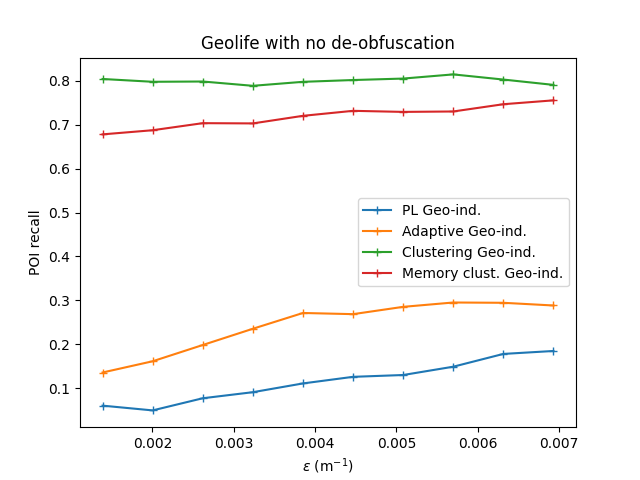
Figure 12. POI recall on Geolife dataset

The POI metric gives us the recall of POIs from the original dataset that can be mapped back from the obfuscated dataset POIs. Looking at Figure 12 we can observe that clustering and memory clustering geo-indistinguishability lead to a high recall of the original POIs. When using clustering or memory clustering geo-indistinguishability the points the user reports are similar to the user’s POIs in number and distribution. Thus, it leads to a high recall. When using PL or adaptive geo-indistinguishability, the points the user reports are spread along the trajectory with some noise. It will be harder to compute the POIs from the obfuscated data, thus leading to a lower recall. This is true for both continuous and sparse datasets (Appendix A).

Figure 3. Average error for the Gowalla dataset (some lines are on top of each other)

The ($\alpha$, $\delta$)-usefulness gives us the distribution of the distance of the obfuscated points from the original point: for every distance $\alpha$ between 0 and 10 km , we compute the proportion $\delta$ of obfuscated points that are within $\alpha$ of their original point. Using the use cases we defined, we can observe the proportion of points that are useful for the user in a given use case. We can observe (Appendix A) that PL, clustering, and memory clustering geo-indistinguishability mechanisms behave similarly for the different datasets. If we consider the local businesses use case ($\alpha$ = 1 km ), for small values of $\epsilon$ (0.00139 m^-1) the proportion of useful points is around 40% and for high values of $\epsilon$ (0.00693 m^-1) the proportion of useful points is almost 100%. The adaptive geo-indistinguishability mechanism is dependent on the distance and the period between the last points. We can observe this dependence, as it performs differently for each dataset. On the Gowalla dataset the proportion of useful points (for $\alpha$ = 1 km) is around 90% for all $\epsilon$ values tested, whereas on the Geolife dataset the proportion of useful points (for $\alpha$ = 1 km) is around 70% for all $\epsilon$ values tested.

4.3. Experiment 2

To gain a better understanding of the influence of the scenario on the privacy and utility of the mechanisms, Experiment 2 is run on the sub-sampled datasets to study the temporal and spatial sampling effect.

Experiment 2 consists in evaluating the privacy and utility of the considered obfuscation mechanisms across different scenarios.

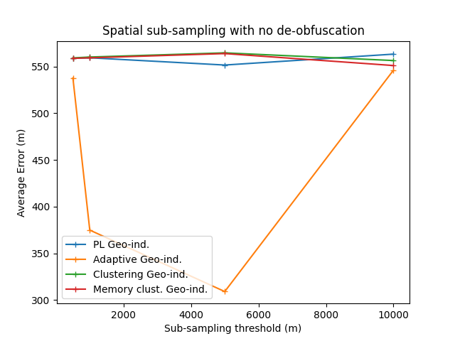
Figure 27. Average error on spatially sub-sampled datasets

Looking at the average error for different values of sub-sampling, we observe that as expected, only adaptive geo-indistinguishability is dependent on the sub-sampling because the other mechanisms apply independently to each point (Figure 27 shows the average error for the spatially sub-sampled datasets).

The POI recall values of the sub-sampled datasets show that, as explained previously, the clustering and memory clustering mechanisms lead to a high recall of the original POIs (high utility). Figure 4 shows the POI recall for temporally sub-sampled datasets for $\epsilon=0.00358$ m^-1. We can observe that the POI recall is higher for sparse datasets (20% POI recall) for PL and adaptive geo-indistinguishability than it is for continuous datasets (50% POI recall).

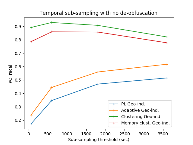
Figure 4. POI recall for the temporally sub-sampled datasets, for $\epsilon=0.00358$ m^-1

If we consider the ($\alpha$, $\delta$)-usefulness graphs for the different scenarios (Appendix A), we can observe that adaptive geo-indistinguishability is the only mechanism to be dependent on the sampling of the dataset. This is coherent with the observations made on the original datasets.

4.4. Experiment 3

To assess the robustness of the obfuscation mechanisms, we carry out in Experiment 3 de-obfuscation attacks on the original datasets obfuscated in different ways accordingly to the mechanism considered.

For the sliding average attack (Appendix A), we can observe that for very sparse datasets (Brightkite and Gowalla) the average error is very high (100s of km) compared to the denser datasets (San Francisco and Geolife). This can be explained by the de-obfuscation mechanism used. We ran the sliding average mechanism by averaging points before and after the current one. Thus, in sparse scenarios, this attack will greatly move the points, whereas in more continuous scenarios the points will not move that much.

The POI recall after a sliding average attack is higher for the PL and adaptive mechanisms (between 60 and 80%) for continuous datasets compared to their recall without any de-obfuscation. For sparse datasets, the POI recalls are overall around 60% for all mechanisms.

For the map matching attack, the average error is bigger (8-10 km) than for sliding average attack (1-2 km ). One explanation could be that the algorithm simply link the points to the nearest possible point in the OpenStreetMap network. Therefore, the points are not necessarily getting closer to the original points after the map matching.

For the POI extraction attack, the average error we observe is on the order of 1 km for continuous datasets but on the order of 20-50 km for sparse datasets. The POIs from the de-obfuscated data are systematically mapped to the closest original POI, therefore for sparse datasets it tends to map them back to POIs that are not as close as the POIs from a continuous dataset.

For the ($\alpha$, $\delta$)-usefulness results, we can see that overall the proportion of useful points after a sliding average attack is higher for continuous datasets (Figure 5) than for sparse datasets (Figure 6). If we consider the local businesses use case ($\alpha$ = 1 km), for all $\epsilon$ values tested, the proportion of useful points is higher for Geolife and San Francisco Cabs datasets. We can even observe a difference between the Geolife dataset (almost 100% of useful points for high values of $\epsilon$) and the San Francisco Cabs dataset (40-50% of useful points for high values of $\epsilon$).

Figure 5. ($\alpha$, $\delta$)-usefulness on San Francisco Cabs dataset (sliding average attack and $\alpha$ = 1000 m)

Figure 6. ($\alpha$, $\delta$)-usefulness on Brightkite dataset (sliding average attack and $\alpha$ = 1000 m)

4.5. Experiment 4

Similarly to what we did earlier in Experiment 2, we now want to study the influence of the scenario on the robustness of the mechanisms. Therefore, we run de-obfuscation attacks on the sub-sampled datasets in Experiment 4.

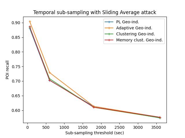
Figure 25. POI recall on temporally sub-sampled datasets with sliding average attack

The POI recall after a sliding average attack goes from 90% for more continuous datasets to 60% for sparser datasets (Figure 25). This confirms the observation on the original datasets: robustness is higher for sparse scenarios.

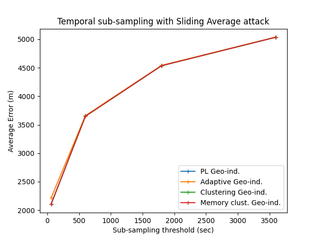
Figure 7. Average error for temporally sub-sampled datasets with sliding average attack (some lines are on top of each other)

The average error after a POI extraction is higher for sparser datasets than it is for more continuous ones (Figure 8). It confirms that for sparse datasets, the POI extraction mechanism tends to match the POIs to original POIs that are further than those for continuous datasets. In this scenario, PL geo-indistinguishability is the most robust mechanism.

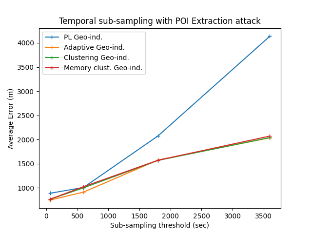
Figure 8. Average error for temporally sub-sampled datasets with POI extraction attack (some lines are on top of each other)

For spatially sub-sampled datasets, we observe that the mechanisms behave similarly. This can be explained by the fact that the clustering radius for clustering and memory clustering geo-indistinguishability is less than the smallest threshold used to sub-sample the San Francisco Cabs dataset. Therefore, these mechanisms cannot create clusters, and they behave just like PL geo-indistinguishability.

The ($\alpha$, $\delta$)-usefulness results (Appendix A) for the sub-sampled datasets confirm that more continuous datasets lead to higher proportion of useful points after a sliding average attack. If we consider the weather forecast use case ($\alpha$ = 10 km) denser datasets have a proportion of almost 100% of useful points, but for sparser datasets the proportion drops to 30% for spatial sub-sampling and 87% for temporal sub-sampling.

4.6. Insights on the Mechanisms

When looking at the results after applying an obfuscation mechanism, but without any de-obfuscation mechanism, we observe that only adaptive geo-indistinguishability is dependent on the scenario of the datasets. This is explained by the way its algorithm works. Overall, the obfuscation mechanisms provided comparable values for average error and ($\alpha$, $\delta$)-usefulness. When looking at the POI recall values, we observe that clustering and memory clustering geo-indistinguishability do not hide very well the POIs compared to the other obfuscation mechanisms. In this regard, we can say that clustering and memory clustering geo-indistinguishability are less private than the other mechanisms. We also observe that PL and adaptive geo-indistinguishability are less private for sparse datasets (50% POI recall) than they are for continuous datasets (20% POI recall).

The results after running the de-obfuscation mechanisms show that overall the error made by the adversary increases when the datasets become sparser for the different attacks. For the POI recall, we observe that when a dataset becomes sparser, the recall decreases after a sliding average attack.

Clustering and memory clustering are less robust against POI extraction attacks, they tend to not hide as much POIs as the other mechanisms. PL geo-indistinguishability is less robust than the other mechanisms against sliding average attacks, while adaptive geo-indistinguishability is often the most robust one in that situation. The privacy, utility, and robustness performances of the mechanisms are dependent on the scenario.

5. Discussion

5.1. Limits

We can identify some limits in our implementation of the framework. For example, our implementation of the map matching algorithm cannot reasonably run on very large datasets, and thus we only run it on the smallest datasets. Moreover, this implementation is simple and could be improved by using Hidden Markov Model for example. For performance reasons, our implementation of the POI extraction mechanism could be optimized by computing the POIs in parallel.

5.2. Future work

The framework can be extended by construction, thus future work could add new mechanisms: new LPPMs not necessarily based on geo-indistinguishability, and new location privacy attacks. Similarly, one could add new metrics to the framework (such as F1-score).

Future work could also be to make this framework more user-friendly. For example, it could be an interactive visualization or website where you could pick datasets with their scenario, mechanisms, and metrics and see the results. It could be helpful for exploration and choice of which mechanism to use to help manufacturers, engineers, etc., make a decision.

After the exploration of the mechanisms and their parameters, the next step is the explainability: by decomposing each mechanism into smaller explainable algorithm, we could for example understand the underlying reasons that make a specific mechanism perform better than another one in a particular scenario.

This deeper understanding could then be leveraged to come up with new and improved mechanisms for location privacy: an automatic shuffling of all components (from the decomposition) could be used to craft maybe a better algorithm.

6. Conclusion

In this paper, we study the sensitivity of geo-indistinguishable obfuscation and de-obfuscation mechanisms on the scenario on which they are used. To study this sensitivity, we introduce an evaluation framework that allows us to systematically evaluate LPPMs by considering an exhaustive combination of LPPMs, attacks, and metrics. Using our framework we compare a selection of LPPMs including an improved mechanism that we introduce. By evaluating over a variety of scenarios, we find that the efficacy of the studied mechanisms vary according to the scenario. For example, we find that the privacy of Planar Laplace geo-indistinguishability is greatly reduced in a continuous scenario (20% points of interest recall) compared to a sparse scenario (45% points of interest recall). We show that the efficacy (privacy, utility, and robustness) that obfuscation and de-obfuscation mechanisms provide is highly dependent on the scenario on which they are used.

Appendix A Graphs

A.1. Brightkite

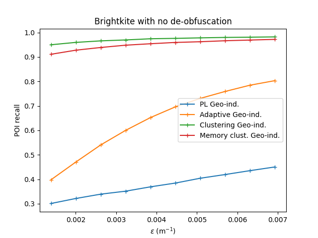
Figure 9. POI recall on Brightkite dataset

Figure 10. Average error on Brightkite dataset

Figure 11. ($\alpha$, $\delta$)-usefulness for $\alpha$ = 10 km on Brightkite dataset with sliding average attack

A.2. Geolife

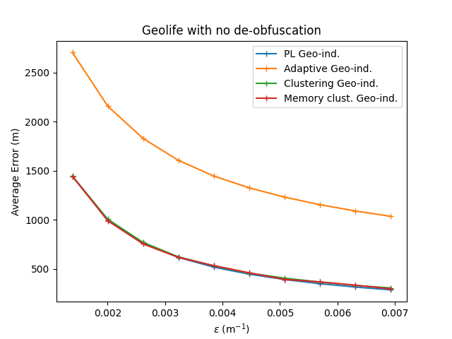
Figure 13. Average error on Geolife dataset

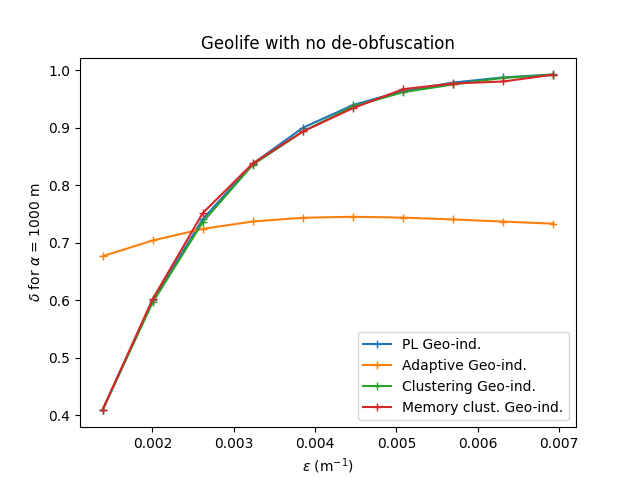
Figure 14. ($\alpha$, $\delta$)-usefulness for $\alpha$ = 1 km on Geolife dataset

Figure 15. ($\alpha$, $\delta$)-usefulness for $\alpha$ = 1 km on Geolife dataset with sliding average attack

A.3. Gowalla

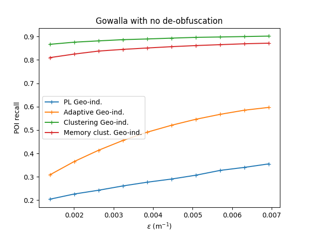
Figure 16. POI recall on Gowalla dataset

Figure 17. Average error on Gowalla dataset

Figure 18. ($\alpha$, $\delta$)-usefulness for $\alpha$ = 1 km on Gowalla dataset with sliding average attack

A.4. San Francisco Cabs

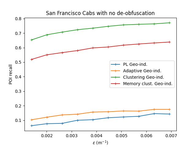
Figure 19. POI recall on San Francisco Cabs dataset

Figure 20. Average error on San Francisco Cabs dataset

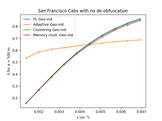
Figure 21. ($\alpha$, $\delta$)-usefulness for $\alpha$ = 500 m on San Francisco Cabs dataset

A.5. Temporally sub-sampled dataset

Figure 22. POI recall on temporally sub-sampled datasets

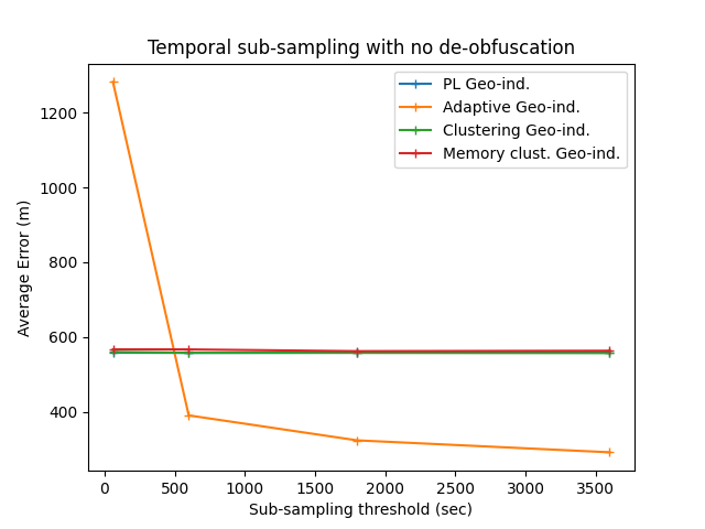
Figure 23. Average error on temporally sub-sampled datasets

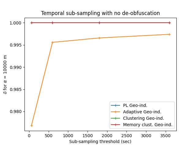
Figure 24. ($\alpha$, $\delta$)-usefulness for $\alpha$ = 10 km on temporally sub-sampled datasets

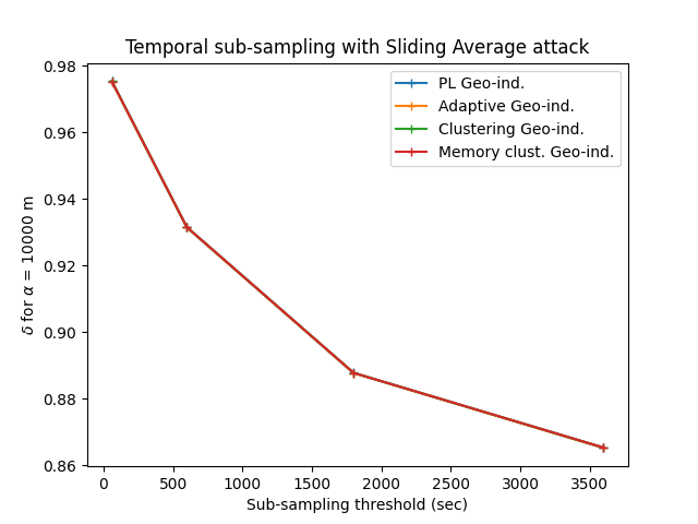
Figure 26. ($\alpha$, $\delta$)-usefulness for $\alpha$ = 10 km on temporally sub-sampled datasets with sliding average attack

A.6. Spatially sub-sampled dataset

Figure 28. ($\alpha$, $\delta$)-usefulness for $\alpha$ = 1 km on spatially sub-sampled datasets

Figure 29. ($\alpha$, $\delta$)-usefulness for $\alpha$ = 10 km on spatially sub-sampled datasets with sliding average attack