A Consistent and Scalable Algorithm for Best Subset Selection in Single Index Models

Abstract

Analysis of high-dimensional data has led to increased interest in both single index models (SIMs) and best subset selection. SIMs provide an interpretable and flexible modeling framework for high-dimensional data, while best subset selection aims to find a sparse model from a large set of predictors. However, best subset selection in high-dimensional models is known to be computationally intractable. Existing methods tend to relax the selection, but do not yield the best subset solution. In this paper, we directly tackle the intractability by proposing the first provably scalable algorithm for best subset selection in high-dimensional SIMs. Our algorithmic solution enjoys the subset selection consistency and has the oracle property with a high probability. The algorithm comprises a generalized information criterion to determine the support size of the regression coefficients, eliminating the model selection tuning. Moreover, our method does not assume an error distribution or a specific link function and hence is flexible to apply. Extensive simulation results demonstrate that our method is not only computationally efficient but also able to exactly recover the best subset in various settings (e.g., linear regression, Poisson regression, heteroscedastic models).

Keywords: Subset Selection Consistency, Single Index Models, High Dimensional Data, Splicing Algorithm, Generalized Information Criterion

1 Introduction

Single index models (SIMs) are simple yet powerful models widely used in statistics and econometrics (Ichimura, 1993; Horowitz and Härdle, 1996). In this paper, we consider a general SIM, where we do not assume the error term is additive with the linear predictor. Formally, suppose $Y\in\mathbb{R}$ is a response variable and $X=(X_{1},\dots,X_{p})^{\top}\in\mathbb{R}^{p}$ are predictors. The model is written as

$$Y=g\left({\boldsymbol{b}}^{\top}X,e\right),$$ (1)

where $\boldsymbol{b}\in\mathbb{R}^{p}$ is the so-called index, $g(\cdot,\cdot)$ is an unknown link function and the error term $e\in\mathbb{R}$ is assumed to be independent of the predictors $X$. Model (1) includes the classical SIM as a special case, which is $Y={g^{\prime}(X\boldsymbol{b})}+e$. Notably, the SIM assumes that the response depends on a linear combination of the predictors through a link function. It is a simple but flexible model, and hence has attracted a great deal of attention (Li and Duan, 1989; Li, 1991; Ichimura, 1993; Horowitz and Härdle, 1996; Kong and Xia, 2007; Xia et al., 2002).

Analysis of high-dimensional data makes SIMs even more appealing because it allows a nonlinear relationship and at the same time, avoids the “curse of dimensionality”, in contrast to linear and nonparametric regression models (Yang et al., 2017; Zhong et al., 2017). However, like linear models, best subset selection is also a fundamental task in SIMs. Despite its importance, best subset selection in high-dimensional SIMs has not been thoroughly studied. This is not surprising because the best subset selection is known as an NP-hard problem and hence computationally infeasible (Natarajan, 1995). Nonetheless, recent advances in statistics and machine learning (Bahmani et al., 2013; Zhu et al., 2020) offer promising ways to tackle the computational intractability. Of particular importance is a splicing algorithm known as adaptive best-subset selection (ABESS, Zhu et al., 2020) that can solve this problem in linear models with a certifiable polynomial complexity. Recently, this algorithm has been extended to generalized linear models (Zhu et al., 2023).

Before presenting our method, we briefly review the related literature, concentrating mainly on the high-dimensional setting. For simultaneous estimation of both the parametric and nonparametric components of SIM, various methods are developed by Alquier and Biau (2013); Radchenko (2015); Luo and Ghosal (2016); Ganti et al. (2017); Cheng et al. (2017). Due to the difficulty of estimating the link function (Eftekhari et al., 2021), substantial efforts have been made to estimate the index vector without estimating the link function (Sheng and Yin, 2013; Zhang and Yin, 2015; Zhong et al., 2017) by maximizing dependence measures. However, variable selection consistency has not been considered in those methods.

Regularization methods for high-dimensional data are known as statistical relaxation of the best subset selection problem. Fan et al. (2022) consider an implicit regularization in over-parameterized SIMs and establish the variable selection consistency, after observing that the direction of $\boldsymbol{b}$ can be obtained from the covariance between $Y$ and a transformation of $X$ (Brillinger, 2012). Before Fan et al. (2022), Neykov et al. (2016); Plan and Vershynin (2016) propose $\ell_{1}$-regularized estimators under Gaussian predictors, and this problem has been further studied by Yang et al. (2017); Na et al. (2019); Wei et al. (2019); Fan et al. (2022) by utilizing Stein’s lemma (Stein et al., 2004). However, these methods make assumptions on both predictors and response that limit their applications.

In contrast, Wang et al. (2012) and Wang and Zhu (2015) propose a rank-based method, which achieves variable selection consistency without any assumptions on the response. Specifically, they simplify the estimation problem to a regularized least square problem and provide support recovery properties for LASSO (Tibshirani, 1996) and non-concave penalty (Fan and Li, 2001), respectively. Wang and Zhu (2015) establish model selection consistency for SIMs in the “$p>n$” scenario. Their method is easy to implement, robust to the error distribution, and achieves certifiable model selection consistency. However, the scalability of this method is limited in high-dimensional cases, as the dimension is only allowed to grow polynomially with the sample size. Furthermore, the stringent irrepresentable condition is proved necessary for model selection consistency (Rejchel and Bogdan, 2020). Rejchel and Bogdan (2020) improve the growth rate of $p$ with respect to $n$ and relax the irrepresentable condition to a cone invertibility factor condition. However, several problems remain open, including the optimal choice of tuning parameters (Rejchel and Bogdan, 2020).

Although the regularization methods are useful in high-dimensional data analysis, several limitations are noteworthy. For instance, the LASSO estimator is known to be biased. While the use of nonconcave penalties addresses the bias issue, the nonconvexity results in challenging computational issues in finding the optimal solution (Huang et al., 2018). Moreover, it is often difficult to select the optimal regularization parameter. Although variable selection methods via regularization have been developed recently, the best subset selection problem itself has not been investigated in high-dimensional SIMs. In this work, we fill the gap by extending the ABESS method of Zhu et al. (2020). Specifically, we propose a rank-based adaptive best-subset selection (RankABESS) algorithm, utilizing the idea of interactively exchanging relevant variables and irrelevant ones until convergence. We demonstrate the scalability of the algorithm by rigorously proving that the algorithm terminates in polynomial times with respect to the sample size and dimension with a high probability. To determine the support size, we adopt a generalized information criterion (GIC) and hence avoid the tuning procedure. Furthermore, we establish desirable statistical properties including the subset selection consistency for our algorithmic solution.

The rest of this paper is organized as follows. In Section 2, we introduce the settings for SIMs. In Section 3, we propose a splicing algorithm, which we refer to as RankABESS, to estimate the index vector up to a constant. Theoretical results for both statistical and computational properties are presented in Section 4. Section 5 includes exhaustive numerical experiments to illustrate the empirical performance of RankABESS. Finally, we conclude with some remarks in Section 6. We provide some additional simulation results in Sections S1 as supplementary materials. Proofs of theoretical results are deferred to Section S2, also as supplementary materials.

2 Notation and Settings

2.1 Notations

Denote by $\mathbf{1}_{n}$ the vector in $\mathbb{R}^{n}$ consisting of all $1$’s. When there is no ambiguity, the subscript $n$ is omitted. For any vector $\boldsymbol{\beta}=(\beta_{1},\dots,\beta_{p})^{\top}\in\mathbb{R}^{p}$, we define the $\ell_{q}$ norm of $\boldsymbol{\beta}$ as $\|\boldsymbol{\beta}\|_{q}=(\sum_{j=1}^{p}\left|\beta_{j}\right|^{q})^{1/q}$ for $q\in\{1,2,\dots\}$. In particular, denote the $\ell_{0}$-norm of $\beta$ as $\|\boldsymbol{\beta}\|_{0}=\sum_{j=1}^{p}\operatorname*{\mathbb{I}}(\beta_{j}\neq 0)$, where $\operatorname*{\mathbb{I}}(\cdot)$ is the indicator function. Let $\mathcal{S}=\{1,\dots,p\}$ be the full index set, and for each set $\mathcal{A}\subseteq\mathcal{S}$, denote $\mathcal{A}^{c}=\mathcal{S}\setminus\mathcal{A}$ as the complement of $\mathcal{A}.$ Define $|\mathcal{A}|$ the carnality of $\mathcal{A}$, and $\boldsymbol{\beta}_{\mathcal{A}}=(\beta_{j},j\in\mathcal{A})\in\mathbb{R}^{|\mathcal{A}|}$. Define the support of a vector $\boldsymbol{\beta}$ as $\operatorname{supp}(\boldsymbol{\beta})=\{j;\beta_{j}\neq 0\}$. For a matrix $\boldsymbol{X}\in\mathbb{R}^{n\times p}$, define $\boldsymbol{X}_{\mathcal{A}}=(\boldsymbol{X}_{j},j\in\mathcal{A})\in\mathbb{R}^{n\times|\mathcal{A}|}$, where $\boldsymbol{X}_{j}$ denotes the $j$-th column of $\boldsymbol{X}$. For any vector $\boldsymbol{u}=(u_{1},\dots,u_{p})\in\mathbb{R}^{p}$ and a index set $\mathcal{A}$, define $\boldsymbol{u}^{\mathcal{A}}$ to be the vector in $\mathbb{R}^{p}$ whose $j$-th element is $u_{j}$ if $j\in\mathcal{A}$ and $0$ otherwise.

2.2 Identification of Index Direction

Model (1) is gnerally not identifiable. In this subsection, we discuss the identification of the index direction. For instance, any shift or scaling of the index vector $\boldsymbol{b}$ can be absorbed into the link function $g$. To identify the index direction, we first assume that $\boldsymbol{b}$ is sparse. Denote $\mathcal{A}^{\star}=\operatorname{supp}(\boldsymbol{b})$ and $\mathcal{I}^{\star}=(\mathcal{A}^{\star})^{c}$ the index sets of relevant and irrelevant predictors, respectively. Let $s^{\star}=|\mathcal{A}^{\star}|$ be the sparsity level. Without loss of generality, we assume that $\operatorname*{\mathbb{E}}X_{j}=0$ for all $j\in\{1,\dots,p\}$. We further assume the following conditions:

1. Denote by $\boldsymbol{\Sigma}$ the population covariance matrix of predictors, i.e. $\boldsymbol{\Sigma}\coloneqq\operatorname*{\mathbb{E}}[XX^{\top}]$. Assume that the covariance matrix of relevant predictors $\boldsymbol{\Sigma}_{\mathcal{A}^{\star},\mathcal{A}^{\star}}$ is invertible. Also, without loss of generality, assume $\Sigma_{jj}=1$ for all $j\in\{1,\dots,p\}$.

2. $\operatorname*{\mathbb{E}}[X_{\mathcal{A}^{\star}}|\boldsymbol{b}_{\mathcal{A}^{\star}}^{\top}{X}_{\mathcal{A}^{\star}}]$ is a linear function of $\boldsymbol{b}_{\mathcal{A}^{\star}}^{\top}{X}_{\mathcal{A}^{\star}}$.

Condition (A1) is commonly used for high-dimensional SIMs (Wang and Zhu, 2015; Wang et al., 2012). It is weaker than the condition in Rejchel and Bogdan (2020) that the whole covariance matrix is invertible. Condition (A2) is a standard condition in the literature of sufficient dimension reduction (Li and Duan, 1989; Li, 1991). It holds for the elliptical distribution such as Gaussian distribution and $t$-distribution. Moreover, as shown in Hall and Li (1993), this condition is not stringent for high-dimensional data because it holds approximately for many data when the dimension tends to infinity.

The following proposition of Wang and Zhu (2015) assures that under the above conditions, the index $\boldsymbol{b}$ is identifiable up to a constant.

Proposition 1

(Wang and Zhu, 2015) Assume Conditions (A1) and (A2) hold, then

$$\boldsymbol{\Sigma}_{\mathcal{A}^{\star},\mathcal{A}^{\star}}^{-1}\operatorname{Cov}\left\{X_{\mathcal{A}^{\star}},\operatorname*{\mathbb{I}}(Y<\tilde{Y})\right\}=\kappa\boldsymbol{b}_{\mathcal{A}^{\star}},$$

where $(\tilde{X},\tilde{Y})$ is an independent copy of $(X,Y)$ and

$$\kappa=\frac{\operatorname*{\mathbb{E}}[\operatorname*{\mathbb{I}}(\tilde{Y}<Y)\boldsymbol{b}_{\mathcal{A}^{\star}}^{\top}X_{\mathcal{A}^{\star}}]}{\boldsymbol{b}_{\mathcal{A}^{\star}}^{\top}\boldsymbol{\Sigma}_{\mathcal{A}^{\star},\mathcal{A}^{\star}}\boldsymbol{b}_{\mathcal{A}^{\star}}}.$$

Proposition 1 enables us to identify the index as $\boldsymbol{\beta}^{\star}$ up to a scalar. Here the intercept and magnitude of the index are not considered since any shift or scaling of the index can be absorbed into the link function $g(\cdot)$.

When $\kappa=0,$ the identifiability becomes an issue (Li, 1991; Wang and Zhu, 2015). This happens, for example, when $g(u,e)=u^{2}+e.$ Despite this, we expect that $\kappa\neq 0$ usually holds. Rejchel and Bogdan (2020) provide a sufficient condition on the link function to guarantee that $\kappa\neq 0.$ From now on, for clarity, we assume that Conditions (A1) and (A2) hold and $\kappa\neq 0$. Moreover for convenience, we let $\boldsymbol{\beta}^{\star}$ denote our target defined by $\boldsymbol{\beta}^{\star}_{\mathcal{A}^{\star}}=-\kappa\boldsymbol{b}_{\mathcal{A}^{\star}}$ and $\boldsymbol{\beta}^{\star}_{\mathcal{I}^{\star}}=\boldsymbol{0}$.

3 Methodology

Having dealt with the identifiability of $\boldsymbol{b},$ we consider the following sample version of SIMs,

$$y_{i}=g\left({\boldsymbol{b}}^{\top}\boldsymbol{x}_{i},{e_{i}}\right),i=1,\dots,n.$$ (2)

Denote $\boldsymbol{y}=(y_{1},\dots,y_{n})$ the response vector, and $\boldsymbol{X}=(\boldsymbol{x}_{1},\dots,\boldsymbol{x}_{n})^{\top}$ the sample design matrix. We further define the rank vector $\boldsymbol{r}=(r_{1},\dots,r_{n})$, where $r_{i}=\sum_{i=1}^{n}\operatorname*{\mathbb{I}}(y_{j}\leq y_{i})$ is the rank of $y_{i}$ in $\boldsymbol{y}.$ Without loss of generality, assume $\boldsymbol{X}$ is centered.

If $\mathcal{A}^{\star}$ is known a prior, Proposition 1 leads to the following natural estimator of $\boldsymbol{\beta}^{\star}_{\mathcal{A}^{\star}},$

$$\hat{\boldsymbol{\beta}}_{\mathcal{A}^{\star}} =-(\frac{1}{n}\boldsymbol{X}_{\mathcal{A}^{\star}}\boldsymbol{X}_{\mathcal{A}^{\star}})^{-1}\left[\frac{1}{n}\sum_{j=1}^{n}\frac{1}{n}\sum_{i=1}^{n}(\boldsymbol{x}_{i})_{\mathcal{A}^{\star}}\operatorname*{\mathbb{I}}\left(y_{i}<y_{j}\right)\right]$$ (3)

$$=(\frac{1}{n}\boldsymbol{X}_{\mathcal{A}^{\star}}\boldsymbol{X}_{\mathcal{A}^{\star}})^{-1}\left[\frac{1}{n}\sum_{i=1}^{n}(\boldsymbol{x}_{i})_{\mathcal{A}^{\star}}\left\{\frac{r_{i}}{n}-1/2\right\}\right]$$

$$=\underset{\operatorname{supp}(\boldsymbol{\beta})\subseteq\mathcal{A}^{\star}}{\operatorname{argmin}}l_{n}(\boldsymbol{\beta}),$$

where

$$l_{n}(\boldsymbol{\beta})\coloneqq\sum_{i=1}^{n}\left(\frac{r_{i}}{n}-1/2-\boldsymbol{x}_{i}^{\top}\boldsymbol{\beta}\right)^{2}.$$

The above estimation procedure leads to an oracle estimator $\hat{\boldsymbol{\beta}}^{o}$, where $\hat{\boldsymbol{\beta}}^{o}_{\mathcal{A}^{\star}}=\hat{\boldsymbol{\beta}}_{\mathcal{A}^{\star}}$ and $\hat{\boldsymbol{\beta}}^{o}_{\mathcal{I}^{\star}}=\boldsymbol{0}$. Statistical properties of $\hat{\boldsymbol{\beta}}^{o}$ are studied in Theorem 3.

In practice, the support of the relevant predictors is usually unknown. Thus, we formulate the estimation problem in the best subset selection paradigm as follows,

$$\min_{\boldsymbol{\beta}}l_{n}(\boldsymbol{\beta}),\textup{ s.t. }\|\boldsymbol{\beta}\|_{0}\leq s.$$ (4)

In general, the best subset selection is known as an NP-hard problem. Recently, Zhu et al. (2020) propose a splicing procedure to solve the $\ell_{0}$-constrained optimization problem efficiently with certifiable statistical properties. This motivates us to propose a rank-based splicing algorithm to solve problem (4). We also provide an information criterion to select the model size to avoid parameter tuning.

For simplicity of notation, denote by $\boldsymbol{C}$ the sample covariance matrix $\boldsymbol{C}\coloneqq\boldsymbol{X}^{\top}\boldsymbol{X}/n$, and define $\boldsymbol{q}=(q_{1},\dots,q_{p})^{\top},$ where $q_{j}=\boldsymbol{X}_{j}^{\top}(\boldsymbol{r}/n-\boldsymbol{1}/2)/n,$ which is the covariance between $\boldsymbol{X}_{j}$ and $\boldsymbol{r}/n,j=1,\ldots,p.$ Similarly, define the correlation vector $\boldsymbol{\rho}=(\rho_{1},\dots,\rho_{p})^{\top},$ where $\rho_{j}=\frac{\boldsymbol{X}_{j}^{\top}(\boldsymbol{r}/n-\boldsymbol{1}/2)}{\lVert\boldsymbol{X}_{j}\rVert_{2}\times\lVert\boldsymbol{r}/n-\boldsymbol{1}/2\rVert_{2}},j=1,\ldots,p.$ For any candidate best subset $\mathcal{A}\subseteq\{1,\dots,p\}$ with carnality $|\mathcal{A}|=s$, denote $\mathcal{I}=\mathcal{A}^{c}.$ We call $\mathcal{A}$ and $\mathcal{I}$ the active set and inactive set, respectively. Given an active set $\mathcal{A}$, we can estimate $\boldsymbol{\beta}$ of support $\mathcal{A}$ with

$$\hat{\boldsymbol{\beta}}=\underset{\operatorname{supp}(\beta)\subseteq\mathcal{A}}{\operatorname{argmin}}l_{n}(\boldsymbol{\beta}).$$

Furthermore, we define two types of sacrifices as follows:

1. Backward sacrifice: $\xi_{j}=l_{n}(\hat{\boldsymbol{\beta}}^{\mathcal{A}\backslash\{j\}})-l_{n}(\hat{\boldsymbol{\beta}}^{\mathcal{A}})=\frac{C_{j,j}}{2}(\hat{\beta}_{j})^{2},\quad\forall j\in\mathcal{A}$

2. Forward sacrifice: $\zeta_{j}=l_{n}(\hat{\boldsymbol{\beta}}^{\mathcal{A}})-l_{n}(\hat{\boldsymbol{\beta}}^{\mathcal{A}}+\hat{\boldsymbol{t}}^{\{j\}})=\frac{(q_{j}-\boldsymbol{X}_{j}^{\top}\boldsymbol{X}\hat{\boldsymbol{\beta}}/n)^{2}}{2C_{j,j}},\quad\forall j\in\mathcal{I}$

where $\hat{\boldsymbol{t}}=\operatorname{argmin}_{\boldsymbol{t}}l_{n}(\hat{\boldsymbol{\beta}}^{\mathcal{A}}+\boldsymbol{t}^{\{j\}})$.

Intuitively, $\xi_{j}$ denotes the magnitude of discarding the $j$-th variable from the active set $\mathcal{A}$, while $\zeta_{j}$ denotes the magnitude of adding the $j$-th variable to the active set. The two types of sacrifices serve as some measures of importance for variables in the active set and inactive set, respectively. Using these sacrifices, the “splicing” algorithm iteratively exchanges the least “important” variables in $\mathcal{A}$ and the most “important” variables in $\mathcal{I}$ until convergence. Given a splicing size $k\leq s$, we define the splicing sets to be

$$\begin{split}\mathcal{S}_{k,1}=\{j\in{\mathcal{A}}:\sum_{i\in{\mathcal{A}}}\operatorname*{\mathbb{I}}(\xi_{j}\geq\xi_{i})\leq k\},\ \mathcal{S}_{k,2}=\{j\in{\mathcal{I}}:\sum_{i\in{\mathcal{I}}}\operatorname*{\mathbb{I}}(\zeta_{j}\leq\zeta_{i})\leq k\},\end{split}$$ (5)

for the active set and inactive set, respectively. By swapping $\mathcal{S}_{k,1}$ and $\mathcal{S}_{k,2}$, we obtain a new active set $\tilde{\mathcal{A}}=(\mathcal{A}\setminus\mathcal{S}_{k,1})\cup\mathcal{S}_{k,2}$ and inactive set $\tilde{\mathcal{I}}=(\tilde{\mathcal{A}})^{c}$. Then based on the new active set, we can obtain $\tilde{\boldsymbol{\beta}}=\operatorname{argmin}_{\operatorname{supp}(\beta)\subseteq\tilde{\mathcal{A}}}l_{n}(\boldsymbol{\beta})$. If $l_{n}(\hat{\boldsymbol{\beta}})-l_{n}(\tilde{\boldsymbol{\beta}})$ is less than the pre-defined threshold, then we update the active set $\mathcal{A}$ by $\tilde{\mathcal{A}}$. We apply the above procedure iteratively until convergence, so the loss function does not decrease more than the pre-defined threshold. We summarize these steps in Algorithm 1.

Algorithm 1 Rank-based Best Subset Selection (RankBESS)

0:  A dataset $\{(\boldsymbol{x}_{i},y_{i})\}^{n}_{i=1}$, the maximum splicing size $k_{\max}$, and a threshold $\tau_{s}$.

1:  Initialize: $\mathcal{A}^{0}=\{j:\sum_{i=1}^{p}\operatorname*{\mathbb{I}}(|\rho_{j}|\leq|\rho_{i}|)\leq s\},\mathcal{I}^{0}=\left(\mathcal{A}^{0}\right)^{c}$ and $\boldsymbol{\beta}_{\mathcal{I}^{0}}^{0}=0$, $\boldsymbol{\beta}_{\mathcal{A}^{0}}^{0}=(C_{\mathcal{A}^{0},\mathcal{A}^{0}})^{-1}\boldsymbol{q}_{\mathcal{A}^{0}}$, $t\leftarrow-1$, $\mathcal{A}^{-1}=\emptyset$.

2:  while $\mathcal{A}^{t+1}\neq\mathcal{A}^{t}$ do

3:     $t\leftarrow t+1$, $\mathcal{A}^{t+1}\leftarrow\mathcal{A}^{t}$, and $L\leftarrow l_{n}(\boldsymbol{\beta}^{t})$.

4:     for $k=1,\ldots,k_{\max}$ do

5:        Compute $\xi_{j}\leftarrow\frac{C_{j,j}}{2}(\beta^{t}_{j})^{2}$ for each $j\in\mathcal{A}^{t}$ and $\zeta_{j}\leftarrow\frac{(q_{j}-\boldsymbol{X}_{j}^{\top}\boldsymbol{X}{\boldsymbol{\beta}^{t}}/n)^{2}}{2C_{j,j}}$ for $j\in\mathcal{I}^{t}$.

6:        Update the candidate active set via splicing: $\tilde{\mathcal{A}}\leftarrow(\mathcal{A}^{t}\backslash\mathcal{S}_{k,1})\cup\mathcal{S}_{k,2}$, where $\mathcal{S}_{k,1},\mathcal{S}_{k,2}$ are computed by (5); and update $\tilde{\mathcal{I}}\leftarrow(\tilde{\mathcal{A}})^{c}$.

7:        Obtain a candidate estimator $\tilde{\boldsymbol{\beta}}$ in which $\tilde{\boldsymbol{\beta}}_{\tilde{\mathcal{A}}}=(\boldsymbol{C}_{\tilde{\mathcal{A}},\tilde{\mathcal{A}}})^{-1}\boldsymbol{q}_{\tilde{\mathcal{A}}},\;\tilde{\boldsymbol{\beta}}_{\tilde{\mathcal{I}}}=0.$

8:        if $L-l_{n}(\tilde{\boldsymbol{\beta}})>\tau_{s}$ then

9:           $L\leftarrow l_{n}(\tilde{\boldsymbol{\beta}})$, $({\mathcal{A}^{t+1}},{\mathcal{I}^{t+1}},{\boldsymbol{\beta}}^{t+1})\leftarrow(\tilde{\mathcal{A}},\tilde{\mathcal{I}},\tilde{\boldsymbol{\beta}})$, and break from the for loop.

10:        end if

11:     end for

12:  end while

12:  $(\boldsymbol{\beta}^{t},\mathcal{A}^{t})$.

Algorithm 2 Rank-based Adaptive Best Subset Selection (RankABESS)

0:  A dataset set $\{(\boldsymbol{x}_{i},y_{i})\}^{n}_{i=1}$ and the maximum support size $s_{\max}$.

1:  for $s=1,\ldots,s_{\max}$ do

2:     $(\hat{\boldsymbol{\beta}}_{s},\hat{\mathcal{A}}_{s})\leftarrow\textbf{RankBESS(s)}\left(\{(\boldsymbol{x}_{i},y_{i})\}^{n}_{i=1},k_{\max},\tau_{s}\right)$.

3:  end for

4:  Compute the size of support set that minimizes the GIC: $\hat{s}\leftarrow\arg\min\limits_{s}\textup{GIC}(\hat{\mathcal{A}}_{s})$.

4:  $(\hat{\boldsymbol{\beta}}_{\hat{s}},\hat{\mathcal{A}}_{\hat{s}})$.

In practice, we determine the support size $s$ by a data driven procedure. Specifically, we use a generalized information criterion (GIC), defined as

$${\operatorname{GIC}(\mathcal{A})=n\min_{\operatorname{supp}(\beta)\subseteq\mathcal{A}}\log l_{n}(\boldsymbol{\beta})+|\mathcal{A}|\log p\operatorname{loglog}n,}$$

to identify the true model. Intuitively, we penalize the model complexity with $\log p$ and prevent underfitting with the slow diverging rate $\operatorname{loglog}n$. Given a maximum support size $s_{\max}$, we apply the above algorithm for $s=1,2,\dots,s_{\max}$ and select the support size such that the $\operatorname{GIC}$ attains the minimum. We state this procedure formally in Algorithm 2. Consistency of this selection procedure will be established in Theorem 2 in the next section. Theorem 2 suggests $s_{\max}=o(\sqrt{\frac{n}{\log p}})$ as the maximum sparsity level, but in practice, we prefer to use $s_{\max}=\Theta(\min\{\sqrt{\frac{n}{\log{p}\operatorname{loglog}{n}}},p\})$.

Remark 1

The key difference between ABESS in Zhu et al. (2020) and RankABESS is that the latter uses the ranks of the response values. This is a very useful technique in robust statistics (Rejchel and Bogdan, 2020) and stablizes the estimation for potentially heavy-tailed responses. Like ABESS, RankABESS retains the scalability for SIMs.

4 Theory

We establish the subset selection consistency of RankABESS in Theorems 1 and 2, and present the computational property of the algorithm in Theorem 4. It is noteworthy that our theory is developed for the algorithmic solution directly and requires no assumption on the error distribution. We will show that our proposed method is certifiably computationally efficient, consistent, and robust to the error distribution.

For notation clarity, let $b^{\star}\coloneqq\min_{j\in\mathcal{A}^{*}}(\beta_{j}^{*})^{2}$ denote the minimum signal strength. We introduce the population version spectrum restricted condition (PSRC). A covariance matrix $\boldsymbol{M}$ satisfies $\operatorname{PSRC}(s,m_{s},M_{s})$ for some constants $m_{s}$ and $M_{s}$, if

$$m_{s}\leq\lambda_{\min}(\boldsymbol{M}_{\mathcal{A},\mathcal{A}})\leq\lambda_{\max}(\boldsymbol{M}_{\mathcal{A},\mathcal{A}})\leq M_{s},\quad\forall\mathcal{A}\text{ with }\lvert\mathcal{A}\rvert\leq s.$$

Below, we describe several conditions that are used in our theoretical results:

1. $\boldsymbol{\Sigma}$ satisfies $\operatorname{PSRC}(2s,m^{0}_{2s},M^{0}_{2s})$ for some constants $m^{0}_{2s}$ and $M^{0}_{2s}$.

   The sample version of spectrum restricted condition (SRC) is commonly assumed in the related literature, see Zhang and Huang (2008); Huang et al. (2018); Zhu et al. (2020). Intuitively, it gives the spectrum bounds for the diagonal submatrices of the covariance matrix. SRC is closely related to the restricted isometry property (RIP) which is known to be less stringent than the irrepresentable condition required for RankLASSO (Rejchel and Bogdan, 2020). Here, We modify SRC to a population version so that it can fit our random predictor setting. Moreover, Condition (C1) implies that the spectrum of the off-diagonal submatrices of the covariance matrix can be upper bounded. Specifically, let $\nu^{0}_{s}$ be the smallest number such that the following inequality holds:

   $$\lambda_{\max}(\boldsymbol{\Sigma}_{\mathcal{A},\mathcal{B}})\leq v^{0}_{s},\quad\forall\lvert\mathcal{A}\rvert\leq s,\lvert\mathcal{B}\rvert\leq s,\mathcal{A}\cap\mathcal{B}=\emptyset.$$

   It follows from Lemma 20 in Huang et al. (2018) that $\nu^{0}_{s}\leq\max\{1-m^{0}_{2s},M^{0}_{2s}-1\}.$

2. For some small constant $\delta_{s}>0$, let $m_{s}=m_{s}^{0}-\delta_{s},$ $M_{s}=M_{s}^{0}+\delta_{s}$, and $\nu_{s}=\nu_{s}^{0}+\delta_{s}$. Assume that there exists some $\Delta>0$ such that

   $$\phi_{s}\coloneqq\frac{2(1+\frac{1+\delta_{s}}{1-\delta_{s}})^{2}M_{s}((1+\Delta)\frac{\nu_{s}}{m_{s}}(1+\frac{\nu_{s}}{m_{s}}))^{2}}{(1-\Delta)(m_{s}-\frac{\nu_{s}^{2}}{m_{s}})}<1.$$

   This technical condition puts some restrictions on the spectrum bounds. This is an analog of Assumption 3 in Zhu et al. (2020). A Similar condition is also assumed in Huang et al. (2018). As discussed in Remark 2 of Zhu et al. (2020), a sufficient condition can be given by $\{m_{2s}\geq 0.8123,M_{2s}\leq 1.8777\}$. Here, we introduce the constant $\delta_{s}$ to control the deviation of the sample covariance matrix from the population version. See Lemma S1 in Section S2 in the supplementary materials for technical details. Besides, it controls the trade-off between the stringency of the assumption and the magnitude of tail probability in our theory.

3. Assume that $x_{1j}$ is univariate subgaussian with coefficient $\omega_{j}$ for all $j\in\mathcal{I}^{\star}$, and $(\boldsymbol{x}_{1})_{\mathcal{A^{\star}}}$ is joint subgaussian with coefficient $\omega_{0}$. Let $\omega=\max\{\omega_{j},\omega_{0},j\in\mathcal{I}^{\star}\}$.

   Condition (C3) is standard in the literature for high-dimensional random design settings (Ravikumar et al., 2011; Rejchel and Bogdan, 2020). Although there are conditions on the distribution of predictors, we do not impose any assumption on the error distribution. In contrast, Yang et al. (2017) and Fan et al. (2022) require assumptions on both predictors and response; that is, $\operatorname*{\mathbb{E}}[y_{1}^{4}]<\infty$ and $\boldsymbol{x}_{1}$ follows a known distribution with density $p_{0}$ in addition to a moment condition on the score function of $\boldsymbol{x}_{1}.$

4. $\tau_{s}=\Theta(\frac{s\log p\operatorname{loglog}n+\sqrt{n\log p}}{n})$.

   Condition (C4) characterizes the magnitude of the threshold that can simultaneously eliminate unnecessary iterations (with the lower bound) and distinguish signals from the random error (with the upper bound). Note that the second term dominates if the sample size is relatively large and vice versa. In particular, if $\frac{s^{2}\log p(\log\log n)^{2}}{n}=o(1)$, $\tau_{s}=\Theta(\sqrt{\frac{\log p}{n}}).$

5. $\frac{s^{2}\log p}{n}=o(1)$.

   Condition (C5) characterizes the maximum growth rate for the support size and the dimension. It is similar to a condition in Zhu et al. (2020) though stronger since a sparser subset is required here to ensure that the sample covariance matrix is close enough to the population version. Similar restrictions are required in Rejchel and Bogdan (2020) for RankLASSO as well. However, this condition is weaker than that in Fan and Tang (2013) for generalized linear models.

6. ${b^{\star}}=\Omega(\frac{s\log p\operatorname{loglog}n+\sqrt{n\log p}}{n})$.

   Condition (C6) characterizes the strength of the minimum signals. Similar conditions are commonly assumed for consistent variable selection in high-dimensional scenarios (Fan and Tang, 2013; Zhu et al., 2020).

7. $\frac{s^{\star}\log p\operatorname{loglog}n}{n}=o(1)$.

   Similar to Condition (C5), Condition (C7) ensures that the order of sparsity level and dimension is not too large. It guarantees the subset selection consistency under the GIC.

8. $\lVert\boldsymbol{\Sigma}_{\mathcal{A}^{\star},\{j\}}\rVert_{2}\times\sqrt{s^{\star}}\leq 1-\delta_{s}$, for all $j\notin\mathcal{A}^{\star}$.

   Condition (C8) imposes a restriction on the correlation between relevant predictors and irrelevant ones. This is weaker than Condition (A2*) in Huang et al. (2018), where a uniform upper bound for the off-diagonal elements of the correlation matrix is assumed. In contrast, we only assume the norm of specific ${|\mathcal{A}^{\star}}|$-length vector is bounded.

Theorem 1 guarantees the consistent subset selection for a given support size by showing that the true active set can be recovered with a high probability, and the recovering probability tends to $1$ as the sample size increases. It also lays the foundation for the consistency under the GIC and guarantees the computational efficiency.

Theorem 1

Assume that Conditions (C1)- (C6) hold, and let $\hat{\mathcal{A}}$ be the estimated active set output by Algorithm 1 for an $s\geq s^{\star}$, then

$$\mathbb{P}(\mathcal{A}^{*}\subseteq\hat{\mathcal{A}})=1-\gamma(s;n,p),$$

where $\gamma(s;n,p)=O\left(p\exp\left\{-nK_{s,1}\frac{b^{\star}}{s}\lor\sqrt{\frac{b^{\star}}{s}}\right\}\right)+O\left(p^{2}\exp\{-K_{s,2}\frac{n}{2s^{2}}\}\right)$ for some constants $K_{s,1}$ and $K_{s,2}$. Asymptotically,

$$\lim_{n\rightarrow\infty}\mathbb{P}(\mathcal{A}^{*}\subseteq\hat{\mathcal{A}})=1.$$

Especially, if $s=s^{\star}$, then we have

$$\lim_{n\rightarrow\infty}\mathbb{P}(\mathcal{A}^{*}=\hat{\mathcal{A}})=1.$$

Remark 2

While Zhu et al. (2020) demonstrate a support recovery property for ABESS in a linear model, we face extra difficulties here due to the interdependence of the ranks of the responses. Furthermore, we make no assumptions about the error distribution. Whereas the support recovery results in Wang and Zhu (2015) presuppose that $s^{\star}=O(n^{c_{1}})$ and $p=o(n^{(c_{2}-2c_{1})k})$ for some $0\leq c_{1}<1/3,2c_{1}<c_{2}\leq 1$ and some positive integer $k$, our results are more lenient in this regard (C5). For the theoretical minimizer of RankLASSO, Rejchel and Bogdan (2020) find a comparable rate. In contrast to their approach, we directly explore aspects of the algorithmic solution here.

Theorem 2 theoretically justifies our support size selection procedure via the GIC. Specifically, our model achieves the subset selection consistency as the sample size increases.

Theorem 2

Assume that Conditions (C1)-(C8) hold with $s_{\max}$. Then, under the GIC, with probability $1-O(p^{-\alpha})$ for some positive constant $\alpha$ and a sufficiently large $n$, the true active set is selected, that is, $\hat{\mathcal{A}}=\mathcal{A}^{*}$.

Remark 3

Model selection consistency for RankLASSO is studied in Wang and Zhu (2015). However, they only allow $p$ increases in a polynomial rate with $n$. Moreover, there is no theoretical guarantees for the tuning parameter selection procedure. In this regard, Rejchel and Bogdan (2020) propose two modified versions: adaptive RankLASSO and thresholded RankLASSO. Although theoretical guidance on tuning parameter selection is provided, it still relies on unknown constants, and the optimal choice of tuning parameter remains unclear. In contrast, we provide a GIC to select the support size with certifiable statistical properties and no need for parameter tuning.

Theorem 2 directly implies that RankABESS leads to the oracle estimator with high probability as shown in the following theorem.

Theorem 3

Assume that the conditions of Theorem 2 hold. Let $\hat{\boldsymbol{\beta}}_{\hat{s}}$ be the output of Algorithm 2. We have

$$P\left(\hat{\boldsymbol{\beta}}_{\hat{s}}=\hat{\boldsymbol{\beta}}^{o}\right)=1-O\left(p^{-\alpha}\right),$$

for some constant $\alpha>0$. Moreover, the following asymptotic properties are achieved.

1. (Consistency) $\lVert\hat{\boldsymbol{\beta}}_{\mathcal{A}^{\star}}-\boldsymbol{\beta}^{\star}_{\mathcal{A}^{\star}}\rVert_{2}=O_{p}(\sqrt{\frac{s^{\star}}{n}})$.

2. (Asymptotic Normality) For any $\boldsymbol{v}\in\mathbb{R}^{p}$ such that $\lVert\boldsymbol{v}\rVert_{2}\leq 1$ and $\boldsymbol{v}^{\top}\boldsymbol{\Omega}\boldsymbol{v}\rightarrow\Lambda$ as $n\rightarrow\infty$ for some $\Lambda>0$ , where $\boldsymbol{\Omega}{\coloneqq\operatorname{Cov}[\boldsymbol{\Sigma}^{-1}_{\mathcal{A}^{\star},\mathcal{A}^{\star}}(F(Y)-1/2-X^{\top}\boldsymbol{\beta}^{\star})X]}$, we have

   $$\sqrt{n}\boldsymbol{v}^{\top}(\hat{\boldsymbol{\beta}}_{\mathcal{A}^{\star}}-\boldsymbol{\beta}^{\star}_{\mathcal{A}^{\star}})\stackrel{{\scriptstyle L}}{{\longrightarrow}}N(0,\Lambda),\quad\text{ as }n\rightarrow\infty.$$

Similar theoretical results for the oracle estimator are developed in Wang et al. (2012). In comparison, we obtain a better rate at the cost of assuming subgaussianity for relevant predictors. Specifically, the $l_{2}$ error bound in probability $O_{p}(\sqrt{\frac{s^{\star}}{n}})$ is tighter than that of Wang et al. (2012). Furthermore, for the asymptotic normality, we require $s^{\star}=o(n^{1/2})$, which is weaker than that in Wang et al. (2012), where $s^{\star}=o(n^{1/4})$ is assumed. Importantly, a direct implication of Theorem 3 is that our estimator enjoys post selection consistency, as shown in the following corollary.

Corollary 1

If the conditions of Theorem 2 hold, we have $\lVert\hat{\boldsymbol{\beta}}_{\hat{s}}-\boldsymbol{\beta}^{\star}\rVert_{2}=o_{p}(1)$.

Following the notation in Algorithm 1, we now turn to the computational properties of RankABESS including an upper bound for the number of iterations of our algorithm in Lemma 1 and a theoretical guarantee for the polynomial complexity in Theorem 4.

Lemma 1

Assume that Conditions (C1)-(C4) hold and $s\geq s^{\star}$. Then with probability at least $1-\gamma(s;n,p)$, at iteration $t,$ we have $\mathcal{A}^{\star}\subseteq\mathcal{A}^{t}$ if

$$t>\log_{\frac{1}{\phi_{s}}}\left(\frac{S_{n}}{n(1-\Delta)(m_{s}-\frac{\nu_{s}^{2}}{m_{s}^{2}})b^{\star}}\right),$$

where $S_{n}\coloneqq\lVert\boldsymbol{r}/n-\mathbf{1}/2\rVert_{2}^{2}=\Theta(n).$

Theorem 4

Assume Conditions (C1) - (C7) hold. Then, with probability $1-O(p^{-\alpha})$ for some positive constant $\alpha$, the computational complexity of RankABESS for a given $s_{\max}$ is

$${O(s_{\max}\log\frac{S_{n}}{\sqrt{n\log p}}+\frac{nS_{n}}{\log p\operatorname{loglog}n})\times(nps_{\max}+ns_{\max}^{2}+k_{\max}ps_{\max}),}$$

where $S_{n}$ is defined in Lemma 1.

Theorem 4 implies that our algorithm achieves a polynomial complexity with high probability. Intuitively, for $s\geq s^{\star}$, Lemma 1 implies that our algorithm recovers the true support within finite iterations. For $s<s^{\star}$, the lower bound in Condition (C4) ensures that unnecessary iterations can be avoided and the computational complexity is also reasonably bounded.

5 Simulation

In this section, we empirically demonstrate the statistical and computational properties of our proposed method which is compared with some state-of-the-art variable selection methods for SIMs. Specifically, the following methods are compared.

• RankABESS: implemented with R package abess (Zhu et al., 2022) The GIC is applied for support size selection.

• RankMCP-CV & RankSCAD-CV: implemented with R package ncvreg, A 10-fold cross-validation (CV) is applied for tuning parameter selection. See Wang et al. (2012).

• RankLASSO-CV: implemented with R package glmnet, 10-fold CV is applied for tuning parameter selection. See Wang and Zhu (2015).

• RankLASSO: implemented with R package glmnet.The parameter tuning follows the method in Rejchel and Bogdan (2020),

• T-RankLASSO & A-RankLASSO: implemented with R package glmnet. The parameter tuning follows the method in Rejchel and Bogdan (2020),

For a fixed dimension $p=2000$, we increase the sample size from 200 to 2000 with equal step size. and investigate the subset selection performance of different methods. The sparsity level is fixed as $10$. We set the true regression coefficient $\boldsymbol{\beta}^{\star}$ as follows. Ten elements equal $2$ and the others are all $0$. The $10$ nonzero coefficients are equally spaced between the $10$-th and $200$-th elements. The predictors are sampled independently from the multivariate Gaussian distribution $\mathcal{MVN}(0,\Sigma)$, where $\Sigma$ is a covariance matrix with three possible choices: the independent structure ($\Sigma=I$), the exponential structure ($\Sigma_{ij}=\rho^{I(i\neq j)}$, where $\rho=0.8$), and the constant structure ($\Sigma_{ij}=\rho$, where $\rho=0.2$). Then we draw the error independently from either the standard Gaussian distribution $N(0,1)$ or the standard Cauchy distribution $t(1)$ and generate response variables from the following two models:

(a) $y_{i}=\boldsymbol{x}_{i}^{\top}\boldsymbol{b}+\boldsymbol{e}_{i}$ (b) $y_{i}=\exp(\boldsymbol{x}_{i}^{\top}\boldsymbol{b})+\boldsymbol{e}_{i}$.

It is noteworthy that RankABESS can also be applied for general single index models, where the error may not be additive with the linear predictor. Additional simulation results for such scenarios can be found in Section S1 of supplementary materials. Performance for subset selection is measured by support recovery probability defined as follows,

1. Recovery probability for the active set: $\mathbb{P}(\mathcal{A}^{*}\subseteq\hat{\mathcal{A}})$.

2. Recovery probability for the inactive set: $\mathbb{P}(\mathcal{I}^{*}\subseteq\hat{\mathcal{I}})$, where $\mathcal{I}^{*}=(\mathcal{A}^{*})^{c}$.

3. Exact support recovery probability: $\mathbb{P}(\mathcal{A}^{*}=\hat{\mathcal{A}})$.

All experiments are based on 100 synthetic datasets. Simulation results for Models (a) and (b) are presented in Figures 1 and 2, respectively.

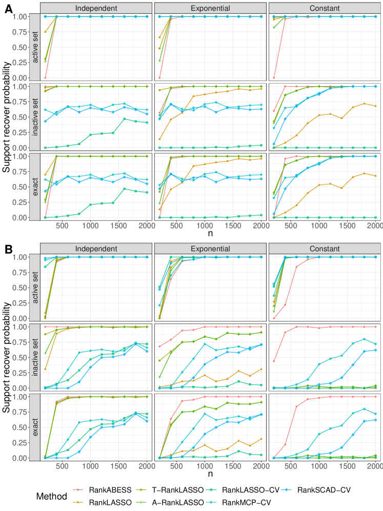
Figure 1: Simulation results for Model (a). Performance for subset selection under different covariance structures and error distributions (A for Gaussian distribution $N(0,1)$, B for Cauchy distribution $t(1)$), measured by support recovery probabilities.

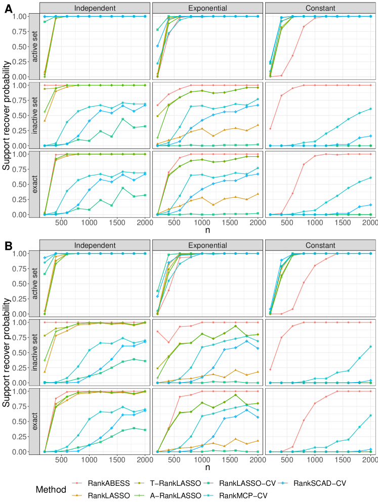
Figure 2: Simulation results for Model (b). Performance for subset selection under different covariance structures and error distributions (A for Gaussian distribution $N(0,1)$, B for Cauchy distribution $t(1)$), measured by support recovery probabilities.

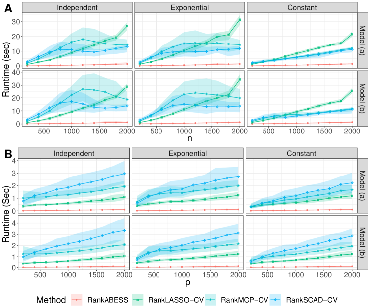
Figure 3: Runtime (in seconds) of RankABESS and CV-based methods in different settings (A for runtime versus $n$, B for runtime versus $p$). The average runtime of 100 replications is recorded. The colored ribbons cover 5%-95% quantiles of runtime for each method.

Model (a).

Under model (a), as depicted by Figure 1A, RankABESS performs competitively in all cases. All methods can cover the active set quite well. However, for exact recovery, only RankABESS, A-RankLASSO and T-RankLASSO achieve consistency in all three $\Sigma$ structures. RankLASSO-CV performs the worst, while RankMCP-CV and RankSCAD-CV perform slightly better for very small $n$ but fail to achieve subset selection consistency as the sample size increases. Since CV procedures provide no guarantees for model selection consistency, these CV-based methods include irrelevant variables occasionally. It is noteworthy that although RankLASSO has similar support recovery performance with A-RankLASSO and T-RankLASSO under the independent $\Sigma$ structure, it fails to achieve consistency under the correlated $\Sigma$ structure. Actually, RankLASSO requires a stringent irrepresentable condition on the design matrix to guarantee consistency, so its poor perforemance is not surprising when the design matrix becomes correlated (Rejchel and Bogdan, 2020). The advantage of RankABESS becomes more apparent in Figure 1B, where the error distribution is heavy-tailed. In this scenario, A-RankLASSO and T-RankLASSO can only recover the true support with probability 1 in the independent correlation $\Sigma$ structure, while RankABESS achieves consistency in all settings.

Model (b).

Figure 2 presents the results under Model (b).The exponential link function challenges the performance of A-RankLASSO and T-RankLASSO. However, RankABESS can still achieve model selection consistency for both Gaussian and Cauchy errors, although relatively larger sample sizes are required for high correlation settings.

In summary, our extensive simulation results demonstrate that RankABESS outperforms other methods for best subset selection in high-dimensional SIMs, achieving the subset selection consistency across various settings, particularly in scenarios with high correlation, heavy-tailed error, and nonlinear link functions.

Using the Cauchy error case as an illustration, we assess the scalability of RankABESS versus the other methods in terms of the runtime. Three CV-based methods are chosen as the benchmark. Figure 3 dispays the runtime: (A) a fixed dimension $p=2000$ and sample sizes ranged from $200$ to $2000$; and (B) with a fixed sample size $n=200$, the dimension increases from $200$ to $2000$. RankABESS is overwhelmingly faster than other methods, which empirically demonstrates the computational efficiency of RankABESS. Moreover, the runtime of RankABESS grows in a linear pattern as the dimension increases when the sample size is fixed, and vice versa. This coincides with Theorem 4, confirming that our algorithm achieves a polynomial complexity.

6 Conclusion and Discussion

In this paper, we propose a novel algorithm, the RankABESS, for best subset selection and index direction estimation in high-dimensional SIMs. To summarize, our contribution is several-fold. First, by adopting the simple rank-based transformation, our method is free of assumptions on the error distribution or the link function and hence has broader applications. Specifically, RankABESS can deal with not only a wide range of models, including generalized linear models, and classical single index models, but also heavy-tailed errors. Second, We rigorously prove that our algorithm can recover the true model for a given model size and that the true model size can be selected under the GIC with high probability, which is further demonstrated by empirical studies. Our proof of the algorithmic properties differs from that in Zhu et al. (2020), owing to new theoretical challenges posed by the dependence among the ranking responses, randomness of predictors, and the absence of assumptions. Third, our algorithm is computationally efficient and capable of high-dimensional datasets in practice. Notably, the scalability of our algorithm is theoretically justified as we rigorously prove that the algorithm has polynomial complexity. To the best of our knowledge, this is the first certifiably polynomial algorithm for best subset selection in SIMs.

Our method has notable advantages over several existing methods. Firstly, it enjoys desirable theoretical properties, similar to the splicing algorithm for linear models or generalized linear models (Zhu et al., 2020), with broader applications. Another recent development in general sparsity constraint optimization is greedy support pursuit (GRASP, Bahmani et al. (2013)). They require a Stable Restricted Hessian or Stable Restricted Linearization condition on the loss function, which imposes constraints on $\boldsymbol{b}$ in addition to those on $X$ and may be stringent in some cases. A weaker but similar condition is also imposed in Zhu et al. (2023). In contrast, such constrants on $\boldsymbol{b}$ are not required for RankABESS. Though both methods can be applied to generalized linear models, RankABESS is simpler in implementation, while GRASP requires a $\ell_{2}$-regularization to avoid singularity in logistic regression, for example. Finally, RankABESS does not require any tricky tuning and has the oracle property with a high probability, while for (modified) RankLASSO, open problems related to tuning parameter selection still exist, and biased estimators are obtained.

A meaningful topic for future study is to extend our method for best subset of groups selection problem, which is useful to analyze variables with certain group structures and has drawn the interest of many researchers (Yuan and Lin, 2006). Recently, a splicing type algorithm has been developed for group best subset selection problem in linear models (Zhang et al., 2023). This paves the way to study best subset of groups selection in SIMs. Another future direction to explore is to alleviate assumptions on the predictors. Although achieving robustness to the error distribution, we pay the cost of imposing the linearity and subgaussianity conditions on the predictors. On the other hand, robust variable selection procedures without restrictive conditions on the predictors have been developed in Wang et al. (2013) and Wang et al. (2020) for linear models, which are inspiring for further studies. In more general settings of empirical risk minimization, Hsu and Sabato (2016) provide an alternative generic proposal for heavy-tailed data.

References

- Alquier and Biau (2013) Alquier, P. and G. Biau (2013). Sparse single-index model. Journal of Machine Learning Research 14(1).
- Bahmani et al. (2013) Bahmani, S., B. Raj, and P. T. Boufounos (2013). Greedy sparsity-constrained optimization. Journal of Machine Learning Research 14(25), 807–841.
- Brillinger (2012) Brillinger, D. R. (2012). A Generalized Linear Model With “Gaussian” Regressor Variables, pp. 589–606. New York, NY: Springer New York.
- Cheng et al. (2017) Cheng, L., P. Zeng, and Y. Zhu (2017). BS-SIM: An effective variable selection method for high-dimensional single index model. Electronic Journal of Statistics 11(2), 3522 – 3548.
- Eftekhari et al. (2021) Eftekhari, H., M. Banerjee, and Y. Ritov (2021). Inference in high-dimensional single-index models under symmetric designs. Journal of Machine Learning Research 22(27), 1–63.
- Fan and Li (2001) Fan, J. and R. Li (2001). Variable selection via nonconcave penalized likelihood and its oracle properties. Journal of the American Statistical Association 96(456), 1348–1360.
- Fan et al. (2022) Fan, J., Z. Yang, and M. Yu (2022). Understanding implicit regularization in over-parameterized single index model. Journal of the American Statistical Association 0(0), 1–14.
- Fan and Tang (2013) Fan, Y. and C. Y. Tang (2013). Tuning parameter selection in high dimensional penalized likelihood. Journal of the Royal Statistical Society. Series B (Statistical Methodology) 75(3), 531–552.
- Ganti et al. (2017) Ganti, R., N. Rao, L. Balzano, R. Willett, and R. Nowak (2017). On learning high dimensional structured single index models. Proceedings of the AAAI Conference on Artificial Intelligence 31(1).
- Hall and Li (1993) Hall, P. and K.-C. Li (1993). On almost Linearity of Low Dimensional Projections from High Dimensional Data. The Annals of Statistics 21(2), 867 – 889.
- Horowitz and Härdle (1996) Horowitz, J. L. and W. Härdle (1996). Direct semiparametric estimation of single-index models with discrete covariates. Journal of the American Statistical Association 91(436), 1632–1640.
- Hsu and Sabato (2016) Hsu, D. and S. Sabato (2016). Loss minimization and parameter estimation with heavy tails. Journal of Machine Learning Research 17(18), 1–40.
- Huang et al. (2018) Huang, J., Y. Jiao, Y. Liu, and X. Lu (2018). A constructive approach to penalized regression. Journal of Machine Learning Research 19(10), 1–37.
- Ichimura (1993) Ichimura, H. (1993). Semiparametric least squares (sls) and weighted sls estimation of single-index models. Journal of Econometrics 58, 71–120.
- Kong and Xia (2007) Kong, E. and Y. Xia (2007). Variable selection for the single-index model. Biometrika 94(1), 217–229.
- Li (1991) Li, K.-C. (1991). Sliced inverse regression for dimension reduction. Journal of the American Statistical Association 86(414), 316–327.
- Li and Duan (1989) Li, K.-C. and N. Duan (1989). Regression analysis under link violation. The Annals of Statistics 17(3), 1009 – 1052.
- Luo and Ghosal (2016) Luo, S. and S. Ghosal (2016). Forward selection and estimation in high dimensional single index models. Statistical Methodology 33, 172–179.
- Na et al. (2019) Na, S., Z. Yang, Z. Wang, and M. Kolar (2019). High-dimensional varying index coefficient models via stein’s identity. Journal of Machine Learning Research 20(152), 1–44.
- Natarajan (1995) Natarajan, B. K. (1995). Sparse approximate solutions to linear systems. SIAM Journal on Computing 24(2), 227–234.
- Neykov et al. (2016) Neykov, M., J. S. Liu, and T. Cai (2016). L1-regularized least squares for support recovery of high dimensional single index models with gaussian designs. Journal of Machine Learning Research 17(87), 1–37.
- Plan and Vershynin (2016) Plan, Y. and R. Vershynin (2016). The generalized lasso with non-linear observations. IEEE Transactions on Information Theory 62(3), 1528–1537.
- Radchenko (2015) Radchenko, P. (2015). High dimensional single index models. Journal of Multivariate Analysis 139, 266–282.
- Ravikumar et al. (2011) Ravikumar, P., M. J. Wainwright, G. Raskutti, and B. Yu (2011). High-dimensional covariance estimation by minimizing -penalized log-determinant divergence. Electronic Journal of Statistics 5, 935 – 980.
- Rejchel and Bogdan (2020) Rejchel, W. and M. Bogdan (2020). Rank-based lasso - efficient methods for high-dimensional robust model selection. Journal of Machine Learning Research 21(244), 1–47.
- Sheng and Yin (2013) Sheng, W. and X. Yin (2013). Direction estimation in single-index models via distance covariance. Journal of Multivariate Analysis 122, 148–161.
- Stein et al. (2004) Stein, C., P. Diaconis, S. Holmes, and G. Reinert (2004). Use of exchangeable pairs in the analysis of simulations. Lecture Notes-Monograph Series 46, 1–25.
- Tibshirani (1996) Tibshirani, R. (1996). Regression shrinkage and selection via the lasso. Journal of the Royal Statistical Society. Series B (Methodological) 58(1), 267–288.
- Wang et al. (2020) Wang, L., B. Peng, J. Bradic, R. Li, and Y. Wu (2020). A tuning-free robust and efficient approach to high-dimensional regression. Journal of the American Statistical Association 115(532), 1700–1714.
- Wang et al. (2012) Wang, T., P.-R. Xu, and L.-X. Zhu (2012). Non-convex penalized estimation in high-dimensional models with single-index structure. Journal of Multivariate Analysis 109, 221–235.
- Wang and Zhu (2015) Wang, T. and L. Zhu (2015). A distribution-based lasso for a general single-index model. Science China Mathematics 58, 109–130.
- Wang et al. (2013) Wang, X., Y. Jiang, M. Huang, and H. Zhang (2013). Robust variable selection with exponential squared loss. Journal of the American Statistical Association 108(502), 632–643.
- Wei et al. (2019) Wei, X., Z. Yang, and Z. Wang (2019). On the statistical rate of nonlinear recovery in generative models with heavy-tailed data. In Proceedings of the 36th International Conference on Machine Learning, Volume 97, pp. 6697–6706.
- Xia et al. (2002) Xia, Y., H. Tong, W. K. Li, and L.-X. Zhu (2002). An adaptive estimation of dimension reduction space. Journal of the Royal Statistical Society: Series B (Statistical Methodology) 64(3), 363–410.
- Yang et al. (2017) Yang, Z., K. Balasubramanian, and H. Liu (2017). High-dimensional non-Gaussian single index models via thresholded score function estimation. In Proceedings of the 34th International Conference on Machine Learning, Volume 70, pp. 3851–3860.
- Yuan and Lin (2006) Yuan, M. and Y. Lin (2006). Model selection and estimation in regression with grouped variables. Journal of the Royal Statistical Society: Series B (Statistical Methodology) 68(1), 49–67.
- Zhang and Huang (2008) Zhang, C.-H. and J. Huang (2008). The sparsity and bias of the Lasso selection in high-dimensional linear regression. The Annals of Statistics 36(4), 1567 – 1594.
- Zhang and Yin (2015) Zhang, N. and X. Yin (2015). Direction estimation in single-index regressions via hilbert-schmidt independence criterion. Statistica Sinica 25, 743–758.
- Zhang et al. (2023) Zhang, Y., J. Zhu, J. Zhu, and X. Wang (2023). A splicing approach to best subset of groups selection. INFORMS Journal on Computing 35(1), 104–119.
- Zhong et al. (2017) Zhong, W., X. Liu, and S. Ma (2017). Variable selection and direction estimation for single-index models via DC-TGDR method. Statistics and Its Interface 11(1), 169–181.
- Zhu et al. (2022) Zhu, J., X. Wang, L. Hu, J. Huang, K. Jiang, Y. Zhang, S. Lin, and J. Zhu (2022). abess: A fast best-subset selection library in Python and R. Journal of Machine Learning Research 23(202), 1–7.
- Zhu et al. (2020) Zhu, J., C. Wen, J. Zhu, H. Zhang, and X. Wang (2020). A polynomial algorithm for best-subset selection problem. Proceedings of the National Academy of Sciences 117(52), 33117–33123.
- Zhu et al. (2023) Zhu, J., J. Zhu, B. Tang, X. Chen, H. Lin, and X. Wang (2023). Best-subset selection in generalized linear models: A fast and consistent algorithm via splicing technique. arXiv preprint.