Lévy distributed fluctuations in the living cell cortex

Abstract

The actomyosin cortex is an active material that provides animal cells with a strong but flexible exterior, whose mechanics, including non-Gaussian fluctuations and occasional large displacements or cytoquakes, have defied explanation. We study the active nanoscale fluctuations of the cortex using high-performance tracking of an array of flexible microposts adhered to multiple cultured cell types. When the confounding effects of static heterogeneity and tracking error are removed, the fluctuations are found to be heavy-tailed and well-described by a truncated Lévy stable distribution over a wide range of timescales and multiple cell types. Notably, cytoquakes appear to correspond to the largest random displacements, unifying all cortical fluctuations into a single spectrum. These findings reinforce the cortex’s previously noted similarity to soft glassy materials such as foams, while the form of the fluctuation distribution will constrain future models of the cytoskeleton.

The actomyosin cortex is a thin sheet of active matter formed from actin filaments, crosslinking proteins and myosin contractile motors existing in a dynamic steady state. After decades of study both in cells [1, 2, 3, 4, 5, 6, 7, 8] and in reconstituted gels [9, 10], the mechanical properties of the actomyosin cortex are well known; it is a tensed, nearly elastic network that resists deformations via a dynamic shear modulus which is a weak power-law of frequency [1, 2, 11, 4, 12, 13, 7, 8]. This sheet undergoes active fluctuations that are super-diffusive [14, 15, 16] and heavy-tailed [17, 18, 8]; but such measurements are confounded by effects such as heterogeneity. More recently, the cortex has also been observed to undergo occasional large displacements in the plane [18, 8, 19], termed cytoquakes. These varied phenomena have not yet been reproduced by a physics-based model. Some models [20, 21, 22] predict power-law shear moduli, but do not explain the non-Gaussian fluctuations. Testing of cytoquake models [23, 24, 25] is limited by the available data. While Fredberg and colleagues [1, 17] have long noted that cytoskeletal networks appear similar to soft glassy materials (SGMs) such as foams and emulsions [26, 27, 28, 29], with both displaying power-law rheology [26, 27, 28, 29, 30, 31, 32], super-diffusive dynamics [29, 30, 31, 32] and non-Gaussian displacements [32], how foams and the cytoskeleton can obey the same physics remains an open question.

Here we report low noise, high statistical power measurements of non-Gaussian lateral fluctuations and cytoquakes of the actomyosin cortex of multiple cell types. We used micropost array detectors (mPADs) consisting of dozens of flexible microposts anchored to cells’ basal cortex. The data from each micropost was rescaled to correct for post-to-post heterogenity, before being pooled together. Analysis of the largest post displacements shows them to resemble the previously reported cytoquakes, and to be indistinguishable from chance fluctuations of the superdiffusive random process describing the rest of the fluctuations. We find that the distribution of all micropost displacements is well described by a Lévy alpha-stable form with an exponential truncation, further reinforcing the notion that cells’ non-Gaussian fluctuations and cytoquakes are a single phenomenon. The lag (or waiting) time dependence of this distribution’s shape is not captured by existing models [33, 25]. We conclude that the Lévy distributed fluctuations are caused by a heavy-tailed distribution of microscopic stresses on cytoskeletal elements, which are released during homeostatic remodeling. Thus, our findings can be used to inform and constrain current and future physical models of the cortex. Remarkably, the displacement distribution we observe closely resembles that recently seen in SGM systems [30, 31, 32], reinforcing the correspondence between SGM and cortical mechanics, and its usefulness as a future modelling approach.

We used a poly(dimethylsiloxane) (PDMS) mPAD device platform [8, 19, 34] consisting of 1.8 $\mu$m diameter microposts on hexagonal lattices with center-to-center spacing 4 $\mu$m. The micropost heights were varied from 9.1 to 5.7 $\mu$m, providing effective spring constants for small lateral deflections $k$ of 5.5–22.3 nN/$\mu$m [35], corresponding to substrate stiffnesses 4.3–17 kPa [36]. The mPAD devices were functionalized to restrict cell adhesion to the micropost tops [37] (See SI Methods [38]).

Figure 1: (a) Schematic of a cell on a micropost array. Cellular traction forces deflect the posts, which are tracked optically. (b) The trajectory of a micropost ($k=15.8$ nN/$\mu$m) coupled to the cortex of a 3T3 cell, over 1,800 s, after time-averaging data recorded at 10 fps to 1 fps. (c) The trajectory of a micropost not coupled to the cell shows the measurement error.

NIH 3T3 fibroblasts (ATCC), human embryonic kidney (HEK) cells (ATCC), human bone osteosarcoma epithelial cells (U2OS), and primary neonatal rat cardiac fibroblasts (CFs) were cultured and seeded on the mPADs as described previously [19]. Cardiac myofibroblasts (CMFs) were produced from the CFs by treatment with TGF-$\beta$1 [19] prior to seeding. Bright field videos of individual cells, of duration 30 minutes, were recorded at 10 frames per second (fps) or 100 fps (HEK and U2OS cells only) [8, 34] (See SI Methods [38]). A previous study [8] suggests that the cortex is stiffer than the micropost spring, allowing us to interpret post deflections as cortical displacements rather than forces. While the posts’ spring restoring force on the cortical displacements must limit the displacement amplitude, such effects have been shown to be small on the time scales studied here [8].

The trajectories of the posts $\mathbf{r}(t)$ were determined by a centroid tracking algorithm [39, 8, 34]. To improve resolution, the post centroids were time averaged to 1 fps, yielding a positional uncertainty of $\Delta x\approx 0.5$ nm. To isolate posts coupled to the cortex, we adapted and refined an approach reported previously [8, 19, 34], using the post trajectories’ mean squared displacements (MSDs), average traction force, displacement range, and non-Gaussian parameter to identify posts coupled to the cell, distinguish cortically-associated posts from stress-fiber-associated posts, and to screen out data contaminated by out-of-focus debris (See SI Methods [38].)

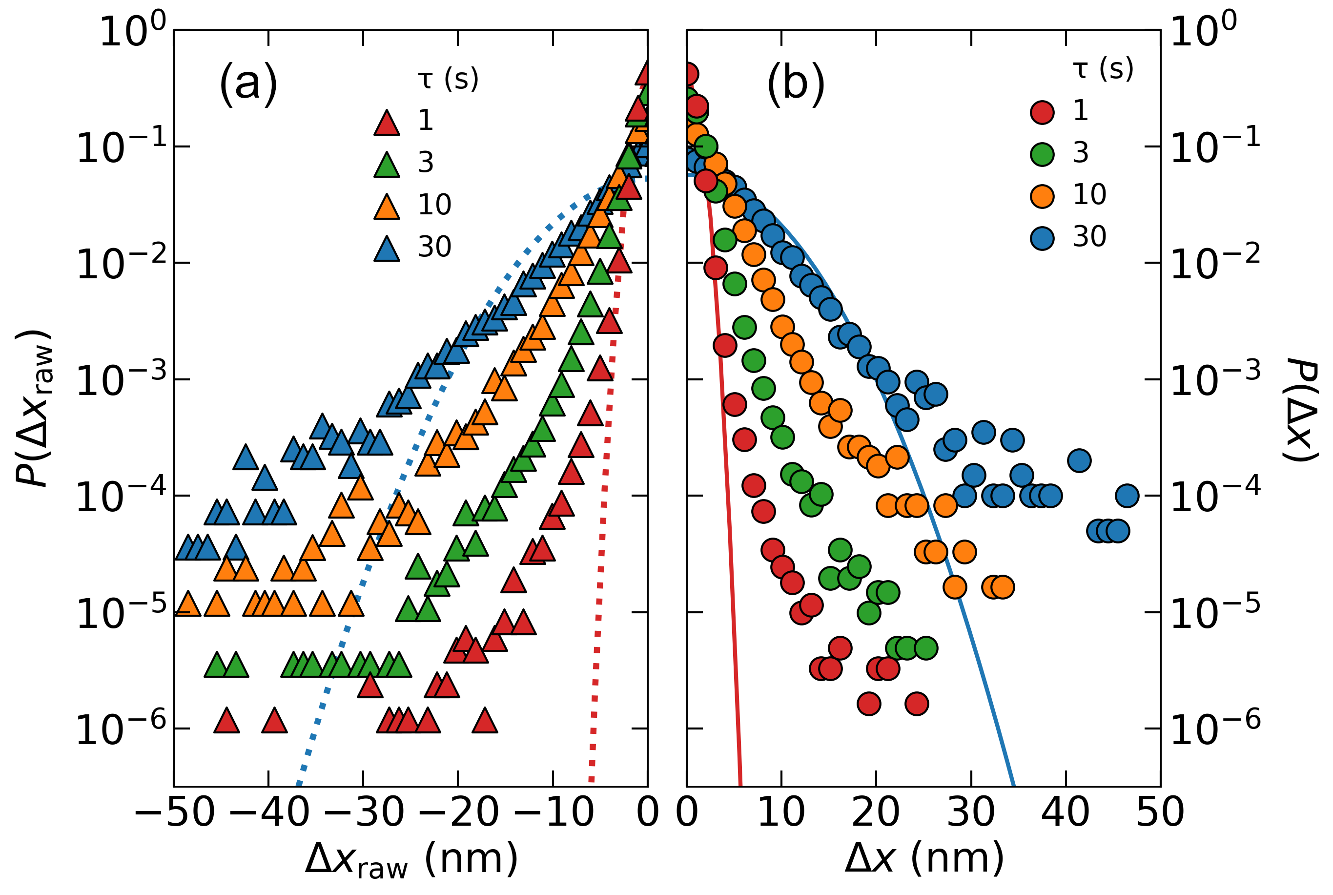
Figure 2: The van Hove displacement distribution is heavy-tailed even after post-to-post heterogeneity is removed. (a) Distribution of measured displacements $P(\Delta x_{\textrm{raw}})$ for the $x$-component of the post trajectories at fixed lag time $\tau$ for an ensemble of 336 posts from nine 3T3 cells. Post stiffness: $k=15.8$ nN/$\mu$m. Only the $\Delta x_{\textrm{raw}}\leq 0$ half of the symmetric distribution is shown, to facilitate comparison with Panel (b). (b) Van Hove distributions $P(\Delta x)$ following rescaling to remove static heterogeneity as described in the text. Only the $\Delta x\geq 0$ half of the symmetric distribution is shown. The lines in (a) and (b) are best-fit Gaussians at $\tau=1\,\textrm{s}$ and $\tau=30\,\textrm{s}$.

Microposts attached to the cell cortex showed dynamic displacements on the 10 nm scale, driven by lateral cortical fluctuations, while background posts did not (Fig. 1(b,c)). To characterize these random post/cortical displacements, we computed the van Hove self correlation function, or the probability distribution of displacements $P(\Delta x_{\textrm{raw}}(\tau))$ in a waiting (or lag) time $\tau$. Figure 2(a) shows the displacement distribution for an ensemble of 336 posts from 9 different 3T3 cells, for 1 s $\leq\tau\leq$ 30 s. At all lag times measured, the distributions were non-Gaussian with pronounced heavy tails at large $|\Delta x_{\textrm{raw}}|$. Such measurements, which pool results over many posts, are susceptible to confounding effects due to heterogeneity [11], such as variations in how different posts/tracers are coupled to the cytoskeleton, or differences between cells. Prior studies of cells’ cortical displacements using single tracers [18, 8], have yielded similar results to Fig. 2(a), suggesting that such fluctuations are not due solely to heterogeneity.

A pooled measurement of displacements can be corrected for heterogeneity by rescaling. In the case of static heterogeneity each post ‘$i$’ reports the time-dependent motion $x^{i}_{\textrm{raw}}(t)$ of a segment of the cortex multiplied by a different, time-independent constant. This suggests that each post’s motion can be rescaled by a single constant so as to have the same typical amplitude as the entire ensemble, e.g.

$$\Delta x^{i}(t)=\Delta x^{i}_{\textrm{raw}}(t)\left[\dfrac{\langle\textrm{GM}(|\Delta x^{i}_{\textrm{raw}}(\tau=10\,\textrm{s})|)\rangle_{\textrm{ens}}}{\textrm{GM}(|\Delta x^{i}_{\textrm{raw}}(\tau=10\,\textrm{s})|)}\right],$$ (1)

where $\textrm{GM}(.)$ designates the geometric mean of a set of numbers, a robust measure of the typical value in heavy-tailed distributions, and $\langle.\rangle_{\textrm{ens}}$ is an ensemble average over all posts. The choice to scale by the displacements at $\tau=10$ s minimized the effects of measurement error while retaining good statistics. A distribution of post rescaling factors is shown in Fig. S2 [38]. A control analysis showed that the rescaling factor was not significantly time dependent over our $30$ minute datasets; cell to cell variations were also small (see SI Methods [38]).

Figure 2(b) shows the pooled distribution of cortical displacements for 3T3 cells, corrected for static heterogeneity, for a range of lag times. This confirms that cortical fluctuations are intrinsically non-Gaussian, while our statistical power allows us to observe that such non-Gaussianity persists to long lag times. At the shortest lag time $\tau=1$ s, we find random displacements that are up to 40 times larger than the geometric mean, similar to reports for cytoquakes [18]. A subset of posts with typical displacements close to that of the background posts was excluded from this analysis (see SI Methods [38]), as they would be dominated by noise.

Our first task is to understand better the nature of the largest displacements forming the heavy tails. Visual examination of the trajectories corresponding to the largest displacements showed two qualitatively different kinds of events. The majority of the events were isotropically directed and showed roughly sigmoidal shapes with typical widths $>1$ s, while other events were very abrupt, with typical widths $<1$ s, and were strongly directed toward the posts’ resting locations (See SI Methods [38]). Examples of such trajectories and their respective angular probability distributions are shown in Fig. S3(a–d) [38]. Given the tendency of the abrupt events to move toward the post resting location, we hypothesize that they are due to transient loading of the cortex by stress fibers followed by detachment and/or de-adhesion events of the micropost from the cell [8]. Given that such processes are not fluctuations within the cortex itself, as might occur due to motor activity or remodeling, we screened the abrupt events out from our analyses below, except where noted.

Figure 3: Averaged scaled trajectories $\langle x_{i,s}(t)\rangle$ for large displacements are well-described by the interpolation-extrapolation function (IEF). (a–d) $\langle x_{i,s}(t)\rangle$ for the $250$ largest non-abrupt displacements at $\tau=10$ s, for 4 different cell types and conditions, as described in the text. Ten individual scaled trajectories $x_{i,s}(t)$ are superimposed in each case (grey). The micropost stiffnesses were: 3T3 and HEK: $k=$ 15.8 nN/$\mu$m; U2OS: $k=$ 5.5 nN/$\mu$m; CF: $k=$ 22.3 nN/$\mu$m. (e) $\langle x_{i,s}(t)\rangle$ for the $100$ largest abrupt displacements for the 3T3 cells shown in (a). Solid lines are fits to the IEF, Eq. 2. (f) The exponents $a_{\textrm{IEF}}$ from fitting the non-abrupt IEFs (circles) and the corresponding MSD exponents $a_{\textrm{MSD}}$ show close agreement. Dashed line: $a_{\textrm{IEF}}=a_{\textrm{MSD}}$. The $a_{\textrm{IEF}}$ exponents for the abrupt displacements (triangles) differ widely from $a_{\textrm{MSD}}$. Error bars are standard errors, estimated from cell-to-cell variations. The individual trajectories in (a)–(e) were chosen at random from the 50 largest (Panels (a–d)) or 20 largest displacements (Panel (e)).

The remaining ‘non-abrupt’ large displacement events bear a strong resemblance to the cytoquakes we and others have observed previously [18, 8, 19]. We seek to determine whether such cytoquakes are a distinct cellular process or if they are merely chance large-amplitude fluctuations in a stationary random trajectory. We tested the latter scenario by averaging short trajectory segments of many large cytoquake displacements together (selected from the heavy tails of the van Hove distribution), and comparing the result with a statistical prediction based on the entire corresponding micropost dataset. The results $\langle x_{i,s}(t)\rangle$ of scaling and averaging the 250 largest non-abrupt displacements at $\tau=10$ s for four different cell types are shown in Fig. 3(a)–(d). During this averaging, the trajectories $x_{i}(t)$ containing each large displacement were rescaled to pass through the points $(-\tau/2,-1/2)$ and $(+\tau/2,+1/2)$, see SI for calculation details [38]. Figure 3(e) shows a similar average of 100 abrupt displacements for comparison. For a stationary random process, the average of short trajectory segments rescaled as in Fig. 3 is predicted by the interpolation-extrapolation function (IEF) [40]. If the MSD of the stationary random process varies as $\textrm{MSD}\sim\tau^{a}$, then the IEF is given by:

$$\textrm{IEF}(t)=\frac{1}{2\tau^{a}}\left(\left\lvert t+\frac{\tau}{2}\right\rvert^{a}-\left\lvert t-\frac{\tau}{2}\right\rvert^{a}\right).$$ (2)

The predicted IEF form, Eq. 2, with the exponent as a free parameter, yields excellent fits to the data, Fig. 3(a–e). The set of exponents for different cell types $\{a_{\textrm{IEF}}\}$ for the non-abrupt events agree well with the corresponding exponents $\{a_{\textrm{MSD}}\}$ for the MSDs of the full trajectory datasets (Fig. 3(f)). (See Fig. S5 for MSD fits [38].) This agreement shows that the process underlying cytoquakes is indistinguishable from that leading to the balance of the cortical fluctuations. In contrast, the IEF exponents for the abrupt events differ significantly from $\{a_{\textrm{MSD}}\}$, confirming our earlier supposition that they were due to a cellular process distinct from the other cortical fluctuations. These findings suggest that, rather than arising from a distinct and potentially rare cellular process, cytoquakes are caused by the same mechanism underlying most or all cortical fluctuations, and which can be described by a superdiffusive, non-Gaussian process.

Figure 4: The Van Hove fluctuation distributions for 3T3 cells are well-described by an ETSD model (solid lines) over lag times $\tau$ from 1–100 s. The best-fit stable distribution (dashed line) shown at $\tau=1$ s does not capture the behavior near the tail. The best-fit Gaussian is shown at $\tau=1$ s for reference (dotted line). The distributions for $\tau>1$ s are progressively offset by factors of $10^{1.5}$. Micropost stiffness: $k=15.8\,\textrm{nm/$\mu$m}$.

Our remaining task is to model the lag-time dependent van Hove distribution that describes the cytoskeletal fluctuations. To do so, we must first screen out the above described abrupt displacements. As the abrupt displacements were predominantly toward the posts’ resting locations, we split the displacements into two sets: one with displacements moving toward the resting location, which we discarded and the other for those moving away from it, which we retained (Fig. S3(e) [38]). Comparing these two sets of data suggests that the abrupt events (in the ‘toward’ set) are responsible for about 20% of total fluctuations on a power basis, see SI Methods [38].

The cortical displacement distribution with abrupt events removed is shown in Fig. 4, plotted in log-log form, for 3T3 cells, and lag times from 1 to 100 s. Other cell types and conditions give similar results. (See Fig. S6 [38].) We find that the cortical fluctuation distribution is well-described by an exponentially-truncated stable distribution (ETSD), given by:

$$P(\Delta x)=AL_{\alpha}(\Delta x;\alpha,\gamma)e^{-\Delta x/\lambda},$$ (3)

where $L_{\alpha}(\Delta x;\alpha,\gamma)$ is the symmetric Lévy alpha-stable distribution [33] with shape parameter $\alpha$ and scale parameter $\gamma$, $A$ is a normalization constant and $\lambda$ is a truncation length. A stable distribution alone is insufficient to describe the data, as illustrated at $\tau=1$ s in Fig. 4. The ability to describe the entire distribution with a single function, versus a sum of different functions, confirms our conclusion that we are observing the displacements of a single random process.

Figure 5: The ETSD fit parameters vs. lag time $\tau$. (a) The shape parameter $\alpha$ varies with substrate stiffness. (b) The shape parameter $\alpha$ depends on the cell type. (c) and (d) The scale parameter $\gamma$ follows a power law with exponent $\approx 0.7$, corresponding to a super-diffusive MSD. The uncertainty in $\gamma$ is smaller than the size of the markers. (e) and (f) The truncation parameter $\lambda$ increases with increasing $\tau$. Error bars are standard errors, estimated from cell-to-cell variations.

The small amplitude of the displacements in Fig. 4 required us to minimize the amount of positional error in our measurements. Nevertheless, such errors do perturb the observed distributions slightly for $\tau<10$ s. (See Fig. S4 [38]). We accounted for this with an inverse Monte Carlo method (see SI Methods [38]) to determine the parameters of a noise-free ETSD distribution that underlies each data set. The solid lines in Fig. 4 show the convolution of the noise-free model ETSDs with the estimated experimental noise distribution at each $\tau$. These calculations describe the cortical displacement distribution very well over the observable range. Analysis of other cell types and conditions shows similar results (Fig. S6 [38]).

The ETSD parameters for all our data, Fig. 5 depend on lag time in a way that is qualitatively similar across cell types and conditions. The shape parameter $\alpha$ appears to depend on cell type, Figs. 5(a–b). It is roughly constant over much of the $\tau$ range, but shows an upturn at short $\tau$. This suggests a tendency toward Gaussian behavior ($\alpha=2$) at very short lag times. The crossover from such Gaussian behavior to an ETSD could correspond to a dynamical timescale in the cytoskeleton, but more data is clearly needed. The scale parameter $\gamma(\tau)$, Figs. 5(c–d) is akin to the standard deviation and grows with $\tau$, as is seen clearly in Fig. 4. The displacement amplitudes are fairly similar across cell types at a given substrate stiffness, with intuitively larger values on the softer substrates. The roughly power-law lag time dependence of $\gamma(\tau)$ with an exponent greater than $0.5$ is consistent with the fluctuation amplitudes growing super-diffusively. The truncation parameter $\lambda(\tau)$, Figs. 5(e–f) which reflects the maximum size of the fluctuations also grows with $\tau$, but more slowly than $\gamma(\tau)$. The ratio $\lambda/\gamma$ decreasing with $\tau$ suggests the displacement distributions’ regression toward a Gaussian at lag times greater than our ability to measure.

Finally, we consider the physical origin of the ETSD fluctuation distributions we observe. Such displacement distributions can be seen in three-dimensional solids, caused by the distance-dependent strain field around a microscopic energy release event [41, 25]. A similar model that accounts for the actual sheet-like geometry of the cortex [25] however, predicts a distribution whose form is not consistent with our findings. Thus, we conclude that our observations likely reflect a corresponding heavy-tailed distribution of tensions or energies in cytoskeletal elements (such as filaments, motors or cross-links), which are abruptly released during homeostatic remodelling processes. The mathematical properties of the Lévy stable distribution would cause mesoscopic fluctuations (such as on our microposts) to have the same stability parameter as the many microscopic events underlying them, and to have a truncated stable form that regresses to a Gaussian only at very long lag times [42]. Previous studies of super-diffusive cortical fluctuations [15, 43, 16] have concluded that they are caused by random stress steps combined with the power-law rheology of the cortex, which would mathematically correspond to fractional Brownian motion [40]. This study adds the insight that those microscopic stress steps have a heavy-tailed amplitude distribution leading to a modified fractional Brownian motion with an ETSD displacement distribution, which is qualitatively similar to recent mathematical models [44, 45].

Our fluctuation measurements suggest that the actomyosin cortex has a broad distribution of stresses on its microscopic constituents, and promises insights into the functional form of that microscopic stress distribution. This finding is both a clue to direct the development of new physical models and a challenge for existing ones to reproduce. We note that our ETSD fluctuation distribution closely resembles that seen in recent experiments on a soft glassy material [32], further supporting the analogy between the cytoskeleton and SGMs [1] and related approaches to model building. Unlike cell rheology curves, which are parameterized by a single, nearly universal exponent [4], the lag time dependent ETSD parameters we measure here are sensitive to cell type-specific details of actomyosin assembly. Further experiments to link these distribution parameters to actomyosin structure and biochemistry should be useful in enabling the refinement of future models.

We thank B. Camley for helpful discussions, C. S. Chen for donation of mPAD masters and T. Schroer for donation of U2OS cells. This work was supported by NSF grants PHY-1915193 and PHY-1915174 and NIH grant HL-127087.

Supplementary information for “Lévy distributed fluctuations in the living cell cortex”

Shankar Sivarajan, Yu Shi, Katherine M. Xiang, Clary Rodríguez-Cruz, Christopher L. Porter

Geran M. Kostecki, Leslie Tung, John C. Crocker, Daniel H. Reich

I Expanded Methods

Micropost array fabrication: Micropost substrates were formed from poly(dimethylsiloxane) (PDMS, Sylgard) [8, 19] via replica molding [37] using PDMS negative molds produced from silicon masters [35]. The tops of the posts were functionalized with fibronectin (Sigma-Aldrich) via microcontact printing to promote specific cellular adhesion and all remaining surfaces of the arrays were passivated with a 0.2% w/v Pluronic F-127 (Thermo Fisher Scientific) solution to prevent non-specific adhesion [37].

Cell culture and data acquisition: All cell lines were cultured as described previously [8, 19]. NIH 3T3 fibroblasts and human embryonic kidney (HEK) cells were obtained from ATCC, and human bone osteosarcoma epithelial cells (U2OS) were a gift from T. Schroer. Primary cardiac fibroblasts (CFs) were extracted from the hearts of neonatal (2 day old) Sprague Dawley rats (Harlan, Indianapolis, IN, USA). All animal procedures were performed in compliance with guidelines set by the Johns Hopkins Committee on Animal Care and Use and all federal and state laws and regulations [19]. The CFs were maintained in a fibroblastic state by treatment with the TGF-$\beta$ receptor I kinase inhibitor SD-208 (Sigma). Cardiac myofibroblasts (CMFs) were produced from the CFs by treatment with TGF-$\beta$1 (R+D Systems) for 48 h.

All cells were seeded on mPAD devices and incubated overnight prior to measurements to allow them to adhere to and spread on the micropost arrays. Bright field videos of 30 min duration were recorded with a Nikon TE-2000E inverted microscope with a 40$\times$ NA $=0.6$ extra-long working distance air objective as described in detail previously [8, 34].

Data reduction and identification of cortically-associated microposts: For the high-resolution studies in this work, we needed to improve our previously described data reduction and analysis methods [34] to measure the microposts’ trajectories, to identify the set of posts coupled to the cortex of each cell, to further reduce experimental noise, and to obtain cleaner sets of cortically-associated microposts. These prior methods were used as a first step, with the addition of multi-frame averaging, to obtain a preliminary set of trajectories and micropost identifications. Briefly, posts were first provisionally assigned as ‘background’ or ‘cell-associated’ based on visual inspection. Then a centroid-based particle-tracking algorithm [39] was used to obtain the position of each post in each video frame. Frame-to-frame drift was provisionally accounted for by subtracting from each post’s trajectory the average displacement of the initial set of background posts in each video frame relative to the initial frame. All post trajectories were then time-averaged to 1 fps to reduce imaging noise.

The individual posts’ mean squared displacements (MSDs) were computed. As the cell-associated posts’ MSDs showed power-law behavior, $MSD\propto\tau^{a}$ for one to two decades in $\tau$, the MSD exponents $a$ for each post were obtained by fitting and subtracting the short-$\tau$ noise floor and averaging the slope of the logarithmic time derivative of the resulting ‘subtracted MSD’ between 5 s $\leq\tau\leq$ 10 s. The condition $a>0.5$ was used to identify cell-associated posts, and $a<0.1$ was used to identify ‘background’ posts not engaged with the cell. To screen out posts that were not engaged with the cell for the entire 1,800 s measurement interval (due to cell motility, for example), we analyzed the MSDs separately for the first and last third of each video. Posts with MSD exponents $<0.5$ for either of those intervals were eliminated from further consideration.

The undeflected positions of the cell-associated posts were then determined by interpolation based on the positions of the background posts, and the cell posts were then provisionally classified into cortex-associated and stress-fiber associated posts based on their average traction force, as described previously [8, 19, 34].

While the above procedure was sufficient for our prior studies [8, 19], the precise measurement of the cortical fluctuations in this work required several improvements. Importantly, a cleaner set of background posts was needed to measure the frame-to-frame drift more accurately, and to determine better the resting locations of the posts cell-associated posts, which enter the process of separating the cortical posts from those coupled to other cytoskeletal structures, such as stress fibers. In our existing procedures, some posts near the periphery of the cells were misclassified. In addition, there were transient optical disturbances that appeared to be caused by debris in the culture medium floating into the field of view, and which could adversely affect the imaging of both cell-associated and background posts.

To remove these effects, we classified the posts based on (i) their displacement range $x_{\textrm{range}}$, defined as the range covered by the $x$-coordinate of a post’s trajectory, and (ii) the non-Gaussian parameter for the trajectory

$$\textrm{NGP}=\frac{\langle(\Delta x_{\textrm{raw}})^{4}\rangle}{3\langle(\Delta x_{\textrm{raw}})^{2}\rangle}-1,$$ (S1)

where $\langle.\rangle$ is the average over the 30 min trajectory. An example of this classification is shown in Fig. S1, which shows both the cortical posts and the background posts for one cell, as provisionally identified at this stage. The background posts were largely clustered, but with outliers that were mixed in with the cortical posts due to either initial mis-classification or the transient optical effects. Cuts on both $x_{\textrm{range}}$ and the NGP, such as those shown in Fig. S1, were made manually for each cell to obtain a cleaner set of background posts (those in the lower left quadrant of Fig. S1) unencumbered by these effects. For some cells, comprising 15% of the initial data set, the optical disturbances affected the majority of the background posts, and such cells were discarded. Occasional posts identified as cortical appeared in the lower left quadrant of Fig. S1 as well. These were discarded from the data set as misidentified.

The mean trajectory of this improved set of background posts was used to re-dedrift the trajectories of all the posts and to refine the cell-associated posts’ undeflected locations. For the latter procedure, each line of posts running along the $[10]$, $[01]$, and $[\bar{1}1]$ directions of the hexagonal lattice was fit by an orthogonal regression on the background posts along that line. The undeflected location of each cell post was estimated as the weighted average of the intersections of the three lattice lines through the post’s position.

The procedure to bifurcate the cell-attached posts into cortical and stress-fiber was repeated to refine the classification using the improved resting locations. In a few cases this bifurcation procedure did not identify a clear cortical region, and these cells were discarded.

In cases where the transient optical disturbances traversed the cell, the disturbances were masked in the cell-attached posts due to the higher activity of those posts, and so the trajectory of these disturbances as tracked in the background posts was extrapolated across the cell, and the affected cortical posts were manually discarded from the data set.

Rescaling of micropost trajectories by the geometric mean: For each post, the geometric mean, the arithmetic mean in log transform space, at a lag time of 10 s, $\textrm{GM}(x)=\exp(\langle\ln x(\tau=10~{}\textrm{s})\rangle)$, of the displacements was calculated. Post-to-post heterogeneity was removed by scaling each post’s steps by the ratio of the mean of the geometric means of the entire ensemble of posts and the post’s geometric mean. See Eq. 1 in the main text

Tests for time-dependence of post-to-post heterogeneity and for cell-to-cell variations: To test for potential time-dependence in the cortical fluctuation distributions due to cellular activity, for each cell type and/or substrate stiffness the raw van Hove distributions pooled over all the posts for each of the individual cells were computed for the first, middle, and last third of the 30-minute video, and these three distributions were compared via a Kolmogorov-Smirnoff test for each cell. To test for cell-to-cell variability, the van Hove distribution for each cell was compared to the pooled distribution of the other cells of the same cell type and substrate stiffness via a Kolmogorov-Smirnoff test.

Removal of low-signal to noise posts: Some cortical posts had very low activity and their trajectories were dominated by measurement noise. To avoid amplifying this noise when scaling such posts’ trajectories to the average geometric mean of the ensemble, posts with a geometric mean less than twice the average geometric mean of the background posts were discarded.

Determination of displacement events’ duration and direction: To identify the subset of the largest steps in the van Hove distributions that were associated with abrupt non-cortical events, the $x$-components of the post’s motion in the forty second interval centered around the time $t_{s}$ of the center of each of the largest steps measured at lag time $\tau=10$ s was fit to a sigmoid curve of the form

$$x(t)=x_{-\infty}+\dfrac{b}{1+e^{-(t-t_{0})/\delta t}}.$$ (S2)

Steps where the widths of the fit sigmoid $\delta t$ were less than 1 second were identified as abrupt events. Steps where the center of the fit sigmoid $t_{0}$ was greater than 8 s away from $t_{s}$ were excluded from this analysis, as such fits did not adequately characterize the step in question.

The direction $\theta$ of the event relative to the post’s undeflected location was determined from $\cos\theta=\Delta{\bf\hat{r}}\cdot{\bf\hat{r}_{0}}$, where $\Delta{\bf\hat{r}}$ is the unit vector in the direction of the step and ${\bf\hat{r}_{0}}$ is the unit vector pointing to the post’s undeflected location from the position of the post at the start of the step, $t=t_{s}-\tau/2$. Note that with this, $\theta=0$ for steps directly toward the resting location.

IEF analysis: Here we seek to determine if a subset of large displacements in a long random trajectory are statistically consistent with the other fluctuations making up the entire trajectory. For example, we want to detect a case where a given trajectory consists of a single stationary random process with a few large steps superimposed upon it at random times due to a distinct process.

To begin, we construct an ‘average cytoquake’ from the largest displacements in the ensemble of micropost trajectories. Specifically, the 30 min trajectories of each micropost were broken into segments of length $\tau$, and a set of segments with the largest magnitude steps $|\Delta x_{i}|=|x(t_{i}+\tau/2)-x(t_{i}-\tau/2)|$ within the ensemble of trajectories were identified. For each segment, after taking $t\rightarrow t-t_{i}$ to center the segment on $t=0$, the portion of that post’s full trajectory in the interval $-3\tau/2\leq t\leq 3\tau/2$ was rescaled as

$$x_{i,s}(t)=\frac{x(t)-x(-\frac{\tau}{2})}{\Delta x_{i}}-\frac{1}{2}.$$ (S3)

Note that this scaling forces each trajectory to pass through the points $(-\tau/2,-1/2)$ and $(+\tau/2,+1/2)$, no matter the sign of $\Delta x_{i}$. The experimental ‘average cytoquake’ was then computed by averaging the scaled trajectories, $\langle x_{i,s}(t)\rangle$, as shown in Fig. 3.

To construct a model for the average cytoquake or displacement trajectory above, we use the interpolation-extrapolation function (IEF) computed in Ref.([40]). If $x(t)$ is a stationary random function that passes through the two points $x(\tau/2)=\Delta x/2$ and $x(-\tau/2)=-\Delta x/2$, the IEF predicts the average scaled trajectory of $x(t)$ to be

$$\textrm{IEF}(t) = \frac{\left\langle x(t)|x(\frac{\tau}{2})-x(-\frac{\tau}{2})=\Delta x\right\rangle}{\Delta x}$$ (S4)

$$= \frac{\left\langle x(t)\left(x(\frac{\tau}{2})-x(-\frac{\tau}{2})\right)\right\rangle}{\left\langle\left(x(\frac{\tau}{2})-x(-\frac{\tau}{2})\right)^{2}\right\rangle}$$ (S5)

$$= \frac{\left\langle\left(x(t)-x(-\frac{\tau}{2})\right)^{2}\right\rangle-\left\langle\left(x(t)-x(\frac{\tau}{2})\right)^{2}\right\rangle}{2\left\langle\left(x(\frac{\tau}{2})-x(-\frac{\tau}{2})\right)^{2}\right\rangle},$$ (S6)

where $\langle x(t)|x(\frac{\tau}{2})-x(-\frac{\tau}{2})=\Delta x\rangle$ is the conditional expectation for $x(t)$ subject to the given $\Delta x$. This equation shows that the IEF and the mean squared displacement (MSD) are mathematically related in a one to one manner. Specifically, if the MSD is a power-law function of the lag time, the predicted IEF function is given by Eq. 2 in the text. While the above formulae were derived for a fractional Brownian process with a Gaussian van Hove distribution [40], we make the conventional assumption that the formulae hold for general stationary non-Gaussian random processes provided they have non-singular variance/MSD (as is the case with our data) due to the Central Limit Theorem.

Removal of abrupt events from displacement distributions: For each lag time $\tau$, the direction of each displacement was classified as either inward, toward the resting location, or outward, away from it. As the abrupt events were predominantly in the ‘toward’ category while the non-abrupt events were isotropically distributed we discarded all the ‘toward’ displacements, and carried out subsequent analysis on the displacements in the ‘away’ category. To estimate the power carried by the abrupt events we computed the fractional energy difference

$$f_{\textrm{abrupt}}=\frac{E_{\textrm{toward}}-E_{\textrm{away}}}{E_{\textrm{toward}}+E_{\textrm{away}}},$$ (S7)

assuming that the energy carried by the fluctuations $E\propto\sum_{i}(\Delta x_{i})^{2}$.

Modeling of van Hove distributions with ETSDs: The determination of the parameters $(\alpha,\gamma,\lambda)$ in the exponentially-truncated stable distribution (ETSD) $P(\Delta x)$ (Eq. 3 in the main text) used to model the van Hove distributions (Figs. 4 and S6) for the final pooled data sets in each experimental configuration at each $\tau$ proceeded in two stages. First, a maximum-likelihood estimation (MLE) technique was used to calculate the best-fit ETSD for the data set, yielding parameters $(\alpha_{\textrm{exp}},\gamma_{\textrm{exp}},\lambda_{\textrm{exp}})$. For the MLE estimation, a simplex optimization method was used to vary $(\alpha_{\textrm{exp}},\gamma_{\textrm{exp}},\lambda_{\textrm{exp}})$ to minimize the negative logarithm of the probability of the data being drawn from an ETSD with those parameters. All calculations were done in Python, but the normalization constant $A$ in the ETSD was computed numerically in Mathematica at each iteration using the Wolfram client library for Python to ensure sufficient precision in the calculated $P(\Delta x)$ for the simplex optimization to reliably obtain the best-fit parameters.

Next, an inverse Monte Carlo method was used to correct for the effects of experimental noise in the van Hove distributions, to determine the underlying true ETSD parameters $(\alpha,\gamma,\lambda)$. A $4\times 4\times 4$ grid in the space of $(\alpha,\gamma,\lambda)$ was constructed. At each of these points, 4 iterations of a Monte Carlo simulation of the ETSD distribution with noise added were performed to produce simulated data sets. The noise was determined from the measured fluctuation spectrum of the background posts at each $\tau$ for each experimental configuration. The set of background posts were those determined as described above (and see Fig. S1). Each of these four simulated data sets was fit via the MLE procedure described above, and the averaged values of the fit parameters were used to create a grid in the space of $(\alpha_{\textrm{exp}},\gamma_{\textrm{exp}},\lambda_{\textrm{exp}})$ which encompassed the measured values determined from the MLE fit to the data. The final values of $(\alpha,\gamma,\lambda)$ corresponding to $(\alpha_{\textrm{exp}},\gamma_{\textrm{exp}},\lambda_{\textrm{exp}})$ were then determined by interpolation. As the calculated values of $\lambda_{\textrm{exp}}$ were somewhat noisy, the interpolation was first carried out separately in the four $\alpha$, $\gamma$ planes at fixed $\lambda$. The values of $\lambda_{\textrm{exp}}$ corresponding to these $\alpha,\gamma$ pairs were then determined by averaging the $\lambda_{\textrm{exp}}$ values from the four closest points on the $(\alpha_{\textrm{exp}},\gamma_{\textrm{exp}})$ grid. We then used linear interpolation on these four points to determine the final values of $(\alpha,\gamma,\lambda)$. The uncertainties in these parameters for the pooled datasets for each cell type or experimental condition were dominated by cell-to-cell variation, and so were estimated by applying this modeling procedure to each cell’s van Hove and calculating the standard error over the group of cells.

II Supplementary figures

Figure S1: Scatter plot of displacement range $x_{\textrm{range}}$ vs non-Gaussian parameter (NGP) following preliminary identification of cortical and background posts (shown here for a single 3T3 cell on a substrate of stiffness $k=15.8\,\textrm{nm/$\mu$m}$). Number of posts: $N_{\textrm{cortical}}=97$; $N_{\textrm{background}}=660$. Based on such distributions, thresholds for $x_{\textrm{range}}$ and the NGP (solid lines) were manually chosen for each cell to isolate a final set of background posts (lower left quadrant) that were subsequently used to dedrift the posts’ trajectories and to obtain the cortical posts undeflected positions.

Figure S2: The probability distribution $P(GM)$ of the geometric means GM of the cortical posts, shown here for a 3T3 cell on a substrate of stiffness $k=15.8\,\textrm{nm/$\mu$m}$, is well-separated from the GM of the background posts. Number of posts: $N_{\textrm{cortical}}=97$; $N_{\textrm{background}}=660$. Cortical posts with geometric means at $\tau=10$ s less than twice the mean of the geometric means of the background posts were discarded from subsequent analysis to avoid undue amplification of experimental noise.

Figure S3: The dominant isotropic fluctuations in the cortex were isolated by separating steps by their direction relative to the posts’ resting locations. (a) Events extended in time with displacements that were isotropically directed in space. (b) Abrupt events directed toward the resting location of the posts. Only the $x$-components of the post trajectories are shown. The arrows in the insets show the magnitude and direction of the event in the interval $-5$ s $\leq t\leq$ 5 s relative to the post’s undeflected position. (c) Inverse widths vs. direction and classification for the 100 largest events. (d) The angular distribution of the two kinds of events ($\theta=0$ is toward the resting location.) (e) Van Hove distributions for events separated by direction relative to the post’s resting location. To remove the abrupt, directed events, we separated the steps by angle relative to the posts’ resting locations, retaining only those with $|\theta|\geq\pi/2$ This figure highlights the importance of this separation, as inclusion of the large directed events would distort the tails of the cortical fluctuation distribution. As indicated in Panel (d), the separation by angle is imperfect, and some residual abrupt events are perforce included in our final data set. However, as the isotropic events were found to carry 80% of the fluctuation energy, this contribution was likely small.

Figure S4: Comparison of the van Hove distributions of background and cortical posts at short lag times $\tau$ indicated that measurement noise was significant at short lag times (shown here for 3T3 cells on a substrate of stiffness $k=15.8\,\textrm{nm/$\mu$m}$). We employed the inverse Monte Carlo method described in the main text to account for such noise contributions in modeling the cortical van Hove distributions.

Figure S5: The MSDs of the displacements for different cell types and substrate stiffnesses were determined using the variances of the van Hove distributions. The MSD exponents $a_{\textrm{MSD}}$ were determined from fits to $\ln\textrm{MSD}=a_{\textrm{MSD}}\ln\tau+b$ over the range 3 s $\leq\tau\leq$ 30 s. The resulting values for $a_{\textrm{MSD}}$ are shown in Fig. 3(f).

Figure S6: The van Hove distributions of the cortical posts at different lag times for different cell types and substrate stiffnesses are all well-described by our model of ETSD plus noise (solid lines). The resulting ETSD parameters $\alpha$, $\gamma$ and $\lambda$ are shown in Fig. 5 in the main text. The best-fit stable distributions (dashed lines) shown at $\tau=1$ s do not capture the behavior near the tails. The histograms for $\tau>1$ s are progressively offset by factors of $10^{1.5}$ in each panel for clarity.

References

- Fabry et al. [2001] B. Fabry, G. N. Maksym, J. P. Butler, M. Glogauer, D. Navajas, and J. J. Fredberg, Scaling the microrheology of living cells, Physical Review Letters 87, 148102 (2001).
- Hoffman et al. [2006] B. D. Hoffman, G. Massiera, K. M. Van Citters, and J. C. Crocker, The consensus mechanics of cultured mammalian cells, Proceedings of the National Academy of Sciences 103, 10259 (2006).
- Solon et al. [2007] J. Solon, I. Levental, K. Sengupta, P. C. Georges, and P. A. Janmey, Fibroblast adaptation and stiffness matching to soft elastic substrates, Biophysical journal 93, 4453 (2007), publisher: Elsevier.
- Hoffman and Crocker [2009] B. D. Hoffman and J. C. Crocker, Cell mechanics: dissecting the physical responses of cells to force, Annual Review of Biomedical Engineering 11, 259 (2009).
- Tee et al. [2011] S.-Y. Tee, J. Fu, C. S. Chen, and P. A. Janmey, Cell shape and substrate rigidity both regulate cell stiffness, Biophysical journal 100, L25 (2011), publisher: Elsevier.
- Vargas-Pinto et al. [2013] R. Vargas-Pinto, H. Gong, A. Vahabikashi, and M. Johnson, The effect of the endothelial cell cortex on atomic force microscopy measurements, Biophysical journal 105, 300 (2013), publisher: Elsevier.
- Rigato et al. [2017] A. Rigato, A. Miyagi, S. Scheuring, and F. Rico, High-frequency microrheology reveals cytoskeleton dynamics in living cells, Nature physics 13, 771 (2017), publisher: Nature Publishing Group UK London.
- Shi et al. [2019] Y. Shi, C. L. Porter, J. C. Crocker, and D. H. Reich, Dissecting fat-tailed fluctuations in the cytoskeleton with active micropost arrays, Proceedings of the National Academy of Sciences 116, 13839 (2019).
- Gardel et al. [2004] M. Gardel, J. Shin, F. MacKintosh, L. Mahadevan, et al., Elastic behavior of cross-linked and bundled actin networks, Science 304, 1301 (2004).
- Mizuno et al. [2007] D. Mizuno, C. Tardin, C. F. Schmidt, and F. C. MacKintosh, Nonequilibrium mechanics of active cytoskeletal networks, Science 315, 370 (2007), publisher: American Association for the Advancement of Science.
- Trepat et al. [2007] X. Trepat, L. Deng, S. S. An, D. Navajas, D. J. Tschumperlin, W. T. Gerthoffer, J. P. Butler, and J. J. Fredberg, Universal physical responses to stretch in the living cell, Nature 447, 592 (2007).
- Balland et al. [2006] M. Balland, N. Desprat, D. Icard, S. Féréol, A. Asnacios, J. Browaeys, S. Hénon, and F. Gallet, Power laws in microrheology experiments on living cells: Comparative analysis and modeling, Physical Review E 74, 021911 (2006).
- Mandadapu et al. [2008] K. K. Mandadapu, S. Govindjee, and M. R. Mofrad, On the cytoskeleton and soft glassy rheology, Journal of Biomechanics 41, 1467 (2008).
- Caspi et al. [2000] A. Caspi, R. Granek, and M. Elbaum, Enhanced diffusion in active intracellular transport, Physical Review Letters 85, 5655 (2000).
- Lau et al. [2003] A. W. Lau, B. D. Hoffman, A. Davies, J. C. Crocker, and T. C. Lubensky, Microrheology, stress fluctuations, and active behavior of living cells, Physical Review Letters 91, 198101 (2003).
- Guo et al. [2014] M. Guo, A. J. Ehrlicher, M. H. Jensen, M. Renz, J. R. Moore, R. D. Goldman, J. Lippincott-Schwartz, F. C. Mackintosh, and D. A. Weitz, Probing the stochastic, motor-driven properties of the cytoplasm using force spectrum microscopy, Cell 158, 822 (2014).
- Bursac et al. [2005] P. Bursac, G. Lenormand, B. Fabry, M. Oliver, D. A. Weitz, V. Viasnoff, J. P. Butler, and J. J. Fredberg, Cytoskeletal remodelling and slow dynamics in the living cell, Nature Materials 4, 557 (2005).
- Alencar et al. [2016] A. M. Alencar, M. S. A. Ferraz, C. Y. Park, E. Millet, X. Trepat, J. J. Fredberg, and J. P. Butler, Non-equilibrium cytoquake dynamics in cytoskeletal remodeling and stabilization, Soft Matter 12, 8506 (2016).
- Shi et al. [2021] Y. Shi, S. Sivarajan, K. M. Xiang, G. M. Kostecki, L. Tung, J. C. Crocker, and D. H. Reich, Pervasive cytoquakes in the actomyosin cortex across cell types and substrate stiffness, Integrative Biology 13, 246 (2021).
- Broedersz et al. [2010] C. P. Broedersz, M. Depken, N. Y. Yao, M. R. Pollak, D. A. Weitz, and F. C. MacKintosh, Cross-link-governed dynamics of biopolymer networks, Physical Review Letters 105, 238101 (2010).
- Mulla et al. [2019] Y. Mulla, F. MacKintosh, and G. H. Koenderink, Origin of slow stress relaxation in the cytoskeleton, Physical Review Letters 122, 218102 (2019).
- Chen et al. [2021] S. Chen, C. P. Broedersz, T. Markovich, and F. C. MacKintosh, Nonlinear stress relaxation of transiently crosslinked biopolymer networks, Physical Review E 104, 034418 (2021).
- Liman et al. [2020] J. Liman, C. Bueno, Y. Eliaz, N. P. Schafer, M. N. Waxham, P. G. Wolynes, H. Levine, and M. S. Cheung, The role of the Arp2/3 complex in shaping the dynamics and structures of branched actomyosin networks, Proceedings of the National Academy of Sciences 117, 10825 (2020).
- Floyd et al. [2021] C. Floyd, H. Levine, C. Jarzynski, and G. A. Papoian, Understanding cytoskeletal avalanches using mechanical stability analysis, Proceedings of the National Academy of Sciences 118, e2110239118 (2021).
- Swartz and Camley [2021] D. W. Swartz and B. A. Camley, Active gels, heavy tails, and the cytoskeleton, Soft Matter 17, 9876 (2021).
- Hébraud and Lequeux [1998] P. Hébraud and F. Lequeux, Mode-coupling theory for the pasty rheology of soft glassy materials, Physical Review Letters 81, 2934 (1998).
- Sollich et al. [1997] P. Sollich, F. Lequeux, P. Hébraud, and M. E. Cates, Rheology of soft glassy materials, Physical Review Letters 78, 2020 (1997).
- Sollich [1998] P. Sollich, Rheological constitutive equation for a model of soft glassy materials, Phys. Rev. E 58, 738 (1998).
- Hwang et al. [2016] H. J. Hwang, R. A. Riggleman, and J. C. Crocker, Understanding soft glassy materials using an energy landscape approach, Nature Materials 15, 1031 (2016).
- Giavazzi et al. [2020] F. Giavazzi, V. Trappe, and R. Cerbino, Multiple dynamic regimes in a coarsening foam, Journal of Physics: Condensed Matter 33, 024002 (2020).
- Lavergne et al. [2022] F. A. Lavergne, P. Sollich, and V. Trappe, Delayed elastic contributions to the viscoelastic response of foams, The Journal of Chemical Physics 156, 154901 (2022).
- Rodríguez-Cruz et al. [2022] C. Rodríguez-Cruz, M. Molaei, A. Thirumalaiswamy, K. Feitosa, V. N. Manoharan, S. Sivarajan, D. H. Reich, R. A. Riggleman, and J. C. Crocker, Experimental observations of fractal landscape dynamics in a dense emulsion, arXiv preprint arXiv:2210.13667 (2022).
- Zaburdaev et al. [2015] V. Zaburdaev, S. Denisov, and J. Klafter, Lévy walks, Reviews of Modern Physics 87, 483 (2015).
- Shi et al. [2022] Y. Shi, S. Sivarajan, J. C. Crocker, and D. H. Reich, Measuring cytoskeletal mechanical fluctuations and rheology with active micropost arrays, Current Protocols 2, e433 (2022).
- Fu et al. [2010] J. Fu, Y.-K. Wang, M. T. Yang, R. A. Desai, X. Yu, Z. Liu, and C. S. Chen, Mechanical regulation of cell function with geometrically modulated elastomeric substrates, Nature Methods 7, 733 (2010).
- Weng and Fu [2011] S. Weng and J. Fu, Synergistic regulation of cell function by matrix rigidity and adhesive pattern, Biomaterials 32, 9584 (2011).
- Tan et al. [2003] J. L. Tan, J. Tien, D. M. Pirone, D. S. Gray, K. Bhadriraju, and C. S. Chen, Cells lying on a bed of microneedles: an approach to isolate mechanical force, Proceedings of the National Academy of Sciences 100, 1484 (2003).
- [38] See supplemental material at [url will be inserted by publisher] for expanded methods and supplementary figures.
- Crocker and Grier [1996] J. C. Crocker and D. G. Grier, Methods of digital video microscopy for colloidal studies, Journal of Colloid and Interface Science 179, 298 (1996).
- Mandelbrot and Van Ness [1968] B. B. Mandelbrot and J. W. Van Ness, Fractional Brownian motions, fractional noises and applications, SIAM Review 10, 422 (1968).
- Cipelletti et al. [2003] L. Cipelletti, L. Ramos, S. Manley, E. Pitard, D. A. Weitz, E. E. Pashkovski, and M. Johansson, Universal non-diffusive slow dynamics in aging soft matter, Faraday discussions 123, 237 (2003).
- Mantegna and Stanley [1994] R. N. Mantegna and H. E. Stanley, Stochastic process with ultraslow convergence to a gaussian: the truncated lévy flight, Physical Review Letters 73, 2946 (1994).
- Mackintosh and Levine [2008] F. Mackintosh and A. Levine, Nonequilibrium mechanics and dynamics of motor-activated gels, Physical Review Letters 100, 018104 (2008).
- Stoev and Taqqu [2004] S. Stoev and M. S. Taqqu, Simulation methods for linear fractional stable motion and farima using the fast fourier transform, Fractals 12, 95 (2004).
- Burnecki and Weron [2010] K. Burnecki and A. Weron, Fractional lévy stable motion can model subdiffusive dynamics, Physical Review E 82, 021130 (2010).