Fractal and Fractional SIS model for syphilis data

Abstract

This work studies the SIS model extended by fractional and fractal derivatives. We obtain explicit solutions for the standard and fractal formulations; for the fractional case, we study numerical solutions. As a real data example, we consider the Brazilian syphilis data from 2011 to 2021. We fit the data by considering the three variations of the model. Our fit suggests a recovery period of 11.6 days and a reproduction ratio ($R_{0}$) equal to 6.5. By calculating the correlation coefficient ($r$) between the real data and the theoretical points, our results suggest that the fractal model presents a higher $r$ compared to the standard or fractional case. The fractal formulation is improved when two different fractal orders with distinguishing weights are considered. This modification in the model provides a better description of the data and improves the correlation coefficient.

Mathematical models are a powerful tool to understand, forecast, and simulate control strategies for disease spread. In mathematical epidemiology, one of the most successful is the compartmental. This model type stores individuals in compartments according to their infection status. In general, the flux among the compartments is described by ordinary differential equations that have high accuracy in reproducing real data. In the classical formulations, the host population is divided into compartments of Susceptible ($S$), Exposed ($E$), Infected ($I$), and Recovery ($R$). Combinations of these compartments lead to the SI, SIS, SIR, and SEIR models used to study the spread of different diseases. For sexual diseases, such as gonorrhoea or syphilis, the adequate model is the SIS. The SIS model describes diseases which not confer immunity after the recovery period. In this work, we study extensions of the SIS model via non-integer differential operators, fractional and fractal. We consider syphilis data from 2011 to 2021, collected in Brazil. Our results show that the fractal order operator is more efficient than the fractional and the standard to fit the considered data. Therefore, our methodology can be extended for different models and diseases to obtain the best description of real data.

I Introduction

After the pioneering work of Kermack and McKendrick Kermack1927 in 1927, many works have considered compartmental models Keeling2008 . This type of model compartmentalises the population into groups according to the infection status, which can be Susceptible ($S$), Exposed ($E$), Infected ($I$), and Recovered ($R$) Bjornstad2018 . The $S$ compartment is related to healthy individuals; $E$ with the infected individuals, but not yet infectious; $I$ with the infectious individuals; and $R$ with the individuals who acquire immunity, permanent or not Batista2021 . The combination of these compartments leads to the SI Allen1994 , SIS Gray2011 , SIR Cooper2020 , SIRS Aguiar2008 , SEIR Brugnago2020 , and SEIRS Michele2022 models.

These models have been successfully applied in several contexts Hethcote2000 , for example in diseases as gonorrhoea yorke1976 , COVID-19 Manchein2020 , HIV Dalal2008 , influenza Dushoff2004 , dengue Aguiar2009 , and others Amaku2021 ; Scarpino2019 ; Olsen1990 ; Keeling1999 ; Altizer2006 ; Galvis2022 ; Machado2021 . In addition to the success in modelling real data, the compartmental models can be easily adapted to study generic situations Bjornstad2020 ; Shea2020 ; Bjornstad2020b . For instance, the SEIR model can be adapted to study the effects of two vaccination doses in a determined population Gabrick2022 . The inclusion of multi-strain in a SIR model describes the data of dengue, and, due to seasonality and multi-strain, the solutions become complex, i.e., chaotic Aguiar2011 . Including seasonality in an SEIRS model can lead to coexistence between chaotic and periodic attractors Gabrick2023 . This coexistence is associated with tipping points, which depend on the control parameter. A tipping point was also found when the network topology is considered in SIS or SIR model Ansari2021 . Despite its simplicity, the SIS model can generate rich solutions, such as Turing patterns, when spatial dynamics are included Guo2019 .

Although we have many possibilities for compartmental models, the appropriate choice of model is made based on considerations consistent with the disease AndersonMay . Some diseases do not confer long-immunity in the infected individuals Saka2014 , such as rota-viruses Dian2021 , sexually transmitted Lynn2004 , bacterial Ghosh2006 ; Feng2020 , and other types of infections Pang2019 ; Misra2011 . For these diseases, the appropriate model is the SIS model Wu2023 ; Hethcote1984 . Considering a SIS model with variable population size, Hethcote and van den Driessche Hethcote1995 obtained persistence, equilibrium, and stability thresholds. Their results suggest that combinations of disease persistence and death rate can cause a decrease to zero in the population size. Furthermore, the endemic point is asymptotically stable for some parameters. However, for other parameter ranges, Hopf bifurcation emerges. Gray et al. Gray2012 studied the effects of environmental noise in a SIS model. They obtained explicit solutions of the stochastic version of the model and compared them with numerical solutions. First, they consider a two-state Markov chain, then generalise the results to a finite one. Additionally, they consider a realistic scenario by considering the parameters of Streptococcus pneumoniae spread in children. The stochastic version of this model was obtained in the previous work Gray2011 . Gao and Ruan  Gao2011 , reported a SIS patch model with variable coefficients. In this formulation, the authors investigated the human movement’s influence on the spread of disease among patches. They performed numerical solutions to study the two patches’ situation. Also, considering the two-patch SIS model, Feng et al. explored the stability and bifurcation Feng2020 .

In an attempt to improve this model, extensions have been proposed, for instance, the stochastic version proposed by Gray et al. Gray2011 or the inclusion of reaction-diffusion terms Sun2020 ; Ge2017 ; Cui2016 ; Cai2015 . An extension that has been gaining much attention is the inclusion of fractional derivatives in the SIS model Wang2023 ; Wu2023 ; Liu2019 ; Hassouna2018 ; Balzoti2020 ; Balzoti2021 ; Xia2009 ; Abuasad2019 ; Hoang2020 ; Liu2021 . Fractional calculus has been advanced in different fields as a powerful approach to incorporate different aspects with extensions of the differential operators to a non-integer order Book01 . Fractional operators have been applied in several scenarios, such as anomalous diffusion metzler2000random ; Book01 ; evangelista2023introduction , anomalous charge transport in semiconductors uchauikin2013fractional , chaos zaslavsky2002chaos , magnetic resonance imaging lenzi2022fractional ; magin2019capturing , and electrical impedance barbero2022time ; bisquert2001theory . In epidemiological models, fractional calculus has been used to extend the differential operators and, consequently, the models Angstmann2021 ; Angstmann2016 ; Sene2020 ; Taghvaei2020 ; Almeida2018 ; Ahmad2020 ; Cai2022 , allowing us to obtain different behaviours connected to the different relaxation processes. An important aspect of fractional calculus is the memory effect Li2018 . Due to the non-locality, memory, and extra degree of freedom, the fractional epidemic models are richer compared to the standard ones Balzoti2020 ; Balzoti2021 .

Despite fractional models gaining much attention, less attention has been devoted to extending the epidemiological models with fractal derivatives. The fractal operators, which use the concept of fractal space Arif2021 , have been applied in many situations, such as porous media Brouers2018 , anomalous diffusion Chen2006 ; Chen2010 , heat conduction Wang2012 , dark energy He2014 , Casimir effect Cheng2013 , and others He2018 ; Zhang2009 . Compared to standard calculus, which considers a continuous space-time, fractal calculus has been shown to be more accurate when fitting the experimental data He2018 .

In this work, we study fractional and propose fractal extensions of the SIS model calibrated with syphilis data from Brazil (available on Ref. dados ) from 2011 to 2021. We consider the SIS model due to its simplicity and adequate description of sexual disease transmission Keeling2008 . However, other models can be employed to study the syphilis spread Roy2016 ; Milner2010 ; Iboi2016 . We consider the simplest form of the SIS model, i.e., without demographic characteristics. We made this simplification considering that birth and death rates are practically constant in the time range considered IBGE . This research is organised as follows. We first present the standard SIS model (Section II), and after that, we analyse the extensions based on the fractional (Section III) and fractal (Section IV) differential operators. In the standard and fractal cases, we obtain analytical expressions. For the fractional case, we consider the numerical integrator Predictor-Evaluate-Corrector-Predictor (PECE) diethelm2005 . Our results suggest that fractal calculus presents a higher correlation coefficient in fitting the real data. Finally, in Section V, we draw our conclusions.

II Standard SIS Model

The SIS model compartmentalises the host population into Susceptible ($S$) and Infected individuals ($I$) Keeling2008 . The $S$ individuals are infected when in contact with $I$; after that, they evolve to the $I$ compartment by a transmission rate $\beta$. Once in the $I$ compartment, the individuals stay by an average time equal to $1/\gamma$, thenceforth they can be reinfected, as schematically represented in Fig. 1.

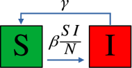
Figure 1: Schematic representation of SIS model.

The standard SIS model is described by the following equations Batista2021

$$\frac{dS}{dt} = -\beta\frac{SI}{N}+\gamma I,$$ (1)

$$\frac{dI}{dt} = \beta\frac{SI}{N}-\gamma I,$$ (2)

subject to the initial conditions $I(0)=I_{0}$ and $S(0)=S_{0}=N-I_{0}$, where $N$, $\beta$, $\gamma$, $S_{0}$, and $I_{0}\geq 0$ Moneim2005 . Therefore, for Eqs. (1) and (2), there exists only one solution for a given initial condition $S_{0}$, $I_{0}$ for all $t\geq 0$, defined in $D=\{(S,I)\in[0,N]^{2}\ |\ S+I=N\}$. The proof of this statement is straightforward using the techniques reported in Hale1969 . In addition, as $S_{0}^{+}$ and $I_{0}^{+}$, we have $S(t)$ and $I(t)\geq 0$ for all $t\geq 0$. The proof is found in Refs. Gao2008 ; Gao2011b .

Equations (1) and (2) are population size dependent. To normalise it, it is necessary to impose the transformations $S\xrightarrow{}sN$ and $I\xrightarrow{}iN$, which are valid for constant population size. As we are considering data from 2011 to 2021, we normalise the model. According to Brazilian Institute of Geography and Statistics (IBGE, Portuguese abbreviation), the Brazilian population increased by around 0.52% per year in the range 2010 to 2022 IBGE ; IBGE2 . In this way, our assumption is reasonable and we can neglect demographic characteristics. With these transformations, the equations are given by

$$\frac{ds}{dt} = -\beta si+\gamma i,$$ (3)

$$\frac{di}{dt} = \beta si-\gamma i,$$ (4)

subject to the initial conditions $i(0)=i_{0}$ and $s(0)=1-i_{0}$. The solutions with biological meaning are restricted to $s,i\in[0,1]$. The sum of Eqs. (3) and (4) results in $s+i=1$. With this constraint, Eq. 4 is rewritten as

$$\frac{di}{dt}=i\beta[1-i-R_{0}^{-1}(t)],$$ (5)

where $R_{0}=\beta/\gamma$ (Ref. Keeling2008 ).

Let $i(0)=i_{0}$, by integration of Eq. 5, we obtain

$$i(t)=\frac{i_{0}\xi e^{\xi\beta t}}{\xi+i_{0}(e^{\xi\beta t}-1)},$$ (6)

where $\xi\equiv(1-R_{0}^{-1})$ and $s(t)$ is immediately determined by $s(t)=1.0-i(t)$. In the limit $t\rightarrow\infty$, Eq. 6 results in $1-R_{0}^{-1}$, which corresponds to the equilibrium state Keeling2008 .

Considering the Brazilian data from syphilis available on Ref. dados , from 2011 to 2021, the best fit suggests $\beta=204.4$, and $\gamma=31.39$ (years^-1). To obtain the best fit, we first calibrate the model by the Levenberg–Marquardt non-linear least-squares algorithm in the R package minpack.lm Elzhov . After that, we compute the correlation coefficient ($r$) between real and simulated data in C language and consider the parameters which maximise $r$. The time evolution of the model with these parameters is shown in Fig. 2(a). These parameters correspond to $R_{0}=6.5$. The real data are not normalised. However, without loss of generality, it is possible to normalise the population in relation to $N=200$ millions (value suggested by the fit). In this case, $i$ gives us information about the fraction of infected each year. As the initial condition, we choose the fraction of infected people in the population at the beginning of the spread, i.e., our initial condition is equal to the initial value $i_{0}=0.0912$. With the $\gamma$ estimated, the average recovery period is equal to 11.6 days, which agrees with syphilis characteristics. For these parameters, the correlation coefficient $r$ is equal to 0.9900. The $r$ value indicates a good fit, which can be seen in Fig. 2(b) by the red line and the experimental points (blue points). The error associated with the explicit solution and the numerical integration (using the Runge-Kutta 4th order method) is $10^{-6}$. This model is very good at fitting the points until 2016. From this point, the theoretical model diverges from the experimental points.

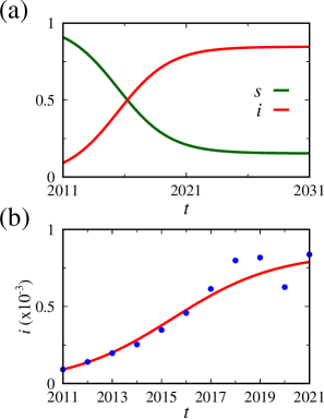
Figure 2: (a) Solution of the SIS model. The green curve is related to $s$ and the red one to $i$. (b) Amplification of $i$ curve in red line and real data in blue points. The correlation coefficient is $r=0.9900$. We consider $\beta=204.4$, $\gamma=31.39$, $R_{0}=6.5$, and $i_{0}=0.0912$. The population is normalised for $N=200$ million.

III Fractional SIS model

To improve the fit of real data, we fix all the parameters found and varied the order of the differential operators to observe if improvement is obtained. As we are dealing with fractions of infected, i.e., normalised population, we can apply the extension directly in the system described by Eqs. 3 and 4. This extension is made by the replacement $\frac{d}{dt}\rightarrow{}\frac{d^{\alpha}}{dt^{\alpha}}$ evangelista2023introduction . In this work, we consider the Caputo fractional operator Book01 , defined by

$$\frac{\partial^{\alpha}}{\partial t^{\alpha}}f(\vec{r},t)=\frac{1}{\Gamma\left(1-\alpha\right)}\int_{0}^{t}dt^{\prime}\frac{1}{(t-t^{\prime})^{\alpha}}\frac{\partial}{\partial t}f(\vec{r},t),$$ (7)

where $\Gamma(\cdot{})$ is the Gamma function, and $\alpha\in(0,1)$. If $\alpha=1$, we recover the usual operator (standard case). Considering the Caputo operator, Eqs. (3) and (4) become

$$\frac{d^{\alpha}s}{dt^{\alpha}} = -\beta si+\gamma i,$$ (8)

$$\frac{d^{\alpha}i}{dt^{\alpha}} = \beta si-\gamma i,$$ (9)

defined in $D=\{(s,i)\in[0,1]^{2}\ |\ s+i=1\}$. Given the initial condition $s_{0}$ and $i_{0}\geq 0$, Eqs. (8) and (9) admit a unique solution $s(t)$ and $i(t)$ Hassouna2018 , which are positive for all $t\geq 0$ Balzoti2021 .

Considering $s+i=1$, Eqs. (5) and (4) are rewritten as

$$\frac{d^{\alpha}i}{dt^{\alpha}}=i\beta[1-i-R_{0}^{-1}].$$ (10)

Due to the nature of fractional operators and the nonlinear aspect of the previous equation, an analytical expression for Eq. (10) as in the previous section is not possible. Numerical solutions are feasible and can be found using the PECE method diethelm2005 . As we are working with Caputo’s definition, the $R_{0}$ is equal to $\beta/\gamma$ and, as all parameters are positive, the solutions stay positive respecting $1=s+i$. Numerical solutions are shown in Fig. 3 for $\alpha=1$ (red line), $\alpha=0.95$ (cyan line), $\alpha=0.90$ (green line), $\alpha=0.85$ (magenta line), and $\alpha=0.75$ (orange line). The respective correlation coefficients are $r=0.9900$, $r=0.9891$, $r=0.9880$, $r=0.9868$, and $r=0.9834$. Note that $r$ decreases as a function of $\alpha$. In this way, no improvement in the fit occurs when fractional operators are considered. This happens because of the nature of the data points. The points increase after 2016, and the fractional derivative slows down the $i$ curve Balzoti2020 . This effect can simulate a control measure in which memory effects are embedded.

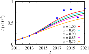
Figure 3: Solutions for the fractional SIS model. The red line is for $\alpha=1$ ($r=0.9900$), cyan line for $\alpha=0.95$ ($r=0.9891$), green line for $\alpha=0.90$ ($r=0.9880$), magenta line for $\alpha=0.85$ ($r=0.9868$), and orange line for $\alpha=0.75$ ($r=0.9834$). We consider $\beta=204.4$, $\gamma=31.39$, $R_{0}=6.5$, and $i_{0}=0.0912$.

IV Fractal model

As the next extension of the model, we consider the fractal derivatives, given by the following definition

$$\frac{df}{dt^{\alpha}}=\frac{1}{\alpha}t^{1-\alpha}\frac{df}{dt}.$$ (11)

This definition is known as Hausdorff derivative He2018 .

For extending the Eqs. (3) and (4) to fractal order, we apply a direct substitution of Eq. (11) into the Eqs., and obtain

$$\frac{ds}{dt} = \alpha t^{\alpha-1}\big{(}-\beta si+\gamma i\big{)},$$ (12)

$$\frac{di}{dt} = \alpha t^{\alpha-1}\big{(}\beta si-\gamma i\big{)},$$ (13)

where $\alpha>0$. Due to the direct connection of fractal derivative with standard one and $t\geq 0$, all the assumptions made for the positive solutions of Eqs. (1) and (2) remain valid for Eqs. (12) and (13). As all parameters are positive, including $t$, the solutions stay preserve $1=s+i$. Similarly to Eq.( 5),

$$\frac{di}{dt}=\alpha t^{\alpha-1}i\beta[1-i-R_{0}^{-1}].$$ (14)

An explicit solution for Eq. (14) is possible and is given by

$$i(t)=\frac{i_{0}\xi e^{\xi\beta t^{\alpha}}}{\xi+i_{0}(e^{\xi\beta t^{\alpha}}-1)},$$ (15)

where $\xi\equiv(1-R_{0}^{-1})$, and $\alpha>0$. The new parameter $\alpha$ is a multiplicative constant, then $R_{0}=\beta/\gamma$.

As a new degree of freedom is included in the model, we expect a better fit of the data set. Figure 4(a) displays $r$ as function of $\alpha$. Differently from the fractional case, the fractal derivative exhibits one point which maximises $r$. This point is $\alpha=0.9673$ and $r=0.99028$. Considering this $\alpha$ value, the solution for the model is shown in Fig. 4(b) by the red line. With this extension, the theoretical model reproduces the data with more precision when compared to the standard and fractional cases. The standard case is recovered when $\alpha\rightarrow 1.$

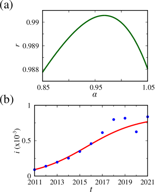
Figure 4: Correlation coefficient as a function of $\alpha$ in the panel (a). Time series for $i$ in the panel (b) for $\alpha=0.9673$, in red line and experimental data in blue points, with $r=0.99028$. We consider $\beta=204.4$, $\gamma=31.39$, $R_{0}=6.5$, and $i_{0}=0.0912$.

Although we improved the fit by including the fractal derivative, the points from 2017 remain away from the red curve. Considering the improvement given by the fractal derivative, we hypothesise that the experimental data are dominated by one fraction, namely $\sigma_{1}$, with weight $a_{1}$ in a certain range of time and, after that, by other fraction $\sigma_{2}$, with the weight $a_{2}$. To include these modifications, we consider $t^{\alpha}\rightarrow a_{1}t^{\sigma_{1}}+a_{2}t^{\sigma_{2}}$, obtaining the expression

$$i(t)=\frac{i_{0}\xi e^{\xi\beta(a_{1}t^{\sigma_{1}}+a_{2}t^{\sigma_{2}})}}{\xi+i_{0}(e^{\xi\beta(a_{1}t^{\sigma_{1}}+a_{2}t^{\sigma_{2}})}-1)},$$ (16)

where $\sigma_{1,2}>0$ and $a_{1,2}$ are real positive constants.

Fixing $\beta=204.4$ and $\gamma=31.39$, the best fit is given for $a_{1}=0.184$, $\sigma_{1}=1.9$, $a_{2}=0.82$, and $\sigma_{2}=0.1$, as can be seen in Fig. 5. Our hypotheses result in $r=0.9980$. The inclusion of two fractal orders modulated the curve behaviour in the different time ranges. For example, for the selected parameters, if we change $a_{1}$ the curve shape changed after 2016. In this way, the first part ($t>2016$) is dominated by $\sigma_{1}$. On the other hand, if we increase or decrease $a_{2}$, the first half of the curve changes for the selected parameters. Due to this characteristic, the SIS model is improved to fit the syphilis Brazilian data. The point located in 2020 diverges from the behaviour, which is not considered in the fit data.

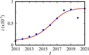
Figure 5: Time series of $i$ in the red line and real data in blue points. We consider $\beta=204.4$, $\gamma=31.39$, $a_{1}=0.184$, $\sigma_{1}=1.9$, $a_{2}=0.82$, and $\sigma_{2}=0.1$. The parameter adjustment is $r=0.9980$.

Figure 6 shows the extension of the $i$ values overtime for the standard case (black line), fractional case with $\alpha=0.9$ (green line), and fractal situation with $a_{1}=0.184$, $\sigma_{1}=1.9$, $a_{2}=0.82$, and $\sigma_{2}=0.1$ (red curve). Superposing these solutions, we show that the fractal model reproduces the data with more precision. Table 1 shows, for the range 2011-2021, the Mean Absolute Error (MAE) equal to 0.05, 0.06, and 0.03 for the standard, fractional, and fractal approaches, respectively. Considering the last point, 2022, the respective MAE changes to 0.09, 0.08, and 0.06. Therefore, our results suggest that the best model to describe the considered data is the fractal one. The last point increases the error due to the fact that we do not employ control measures. This point is in 2022 and can be associated with social behaviour changes or measures of error during the pandemic Wu2023 . To better fit the social behaviour, it is necessary to change $\beta$ or the respective fractional order. As our goal is to reproduce and explains the previous data, we do not take into account control measures, which will be considered in future works.

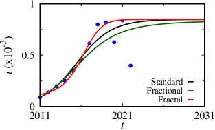
Figure 6: Comparison among the three models versus data points. Standard case (black line), the fractional case with $\alpha=0.9$ (green line), and fractal situation with $a_{1}=0.184$, $\sigma_{1}=1.9$, $a_{2}=0.82$, and $\sigma_{2}=0.1$ (red curve). We consider $\beta=204.4$, $\gamma=31.39$, $R_{0}=6.5$, and $i_{0}=0.0912$.

$\times 10^{-3}$	2011	2012	2013	2014	2015	2016	2017	2018	2019	2020	2021	2022	MAE 11-21 (22)
Data	0.0912	0.1397	0.1966	0.2530	0.3476	0.4575	0.6142	0.7986	0.8176	0.6257	0.8376	0.3979
Standard	0.0912	0.1375	0.2011	0.2824	0.4771	0.5712	0.6511	0.7132	0.7582	0.7893	0.8099	0.8233
Error	0	0.0022	0.0045	0.0294	0.1295	0.1137	0.0369	0.0854	0.0594	0.1636	0.0277	0.4254	0.05 (0.09)
Fractional	0.0912	0.1407	0.2009	0.2735	0.3549	0.4387	0.5181	0.5878	0.6452	0.6905	0.7251	0.7511
Error	0	0.0010	0.0043	0.0205	0.0073	0.0188	0.0961	0.2108	0.1724	0.0648	0.1125	0.3532	0.06 (0.08)
Fractal	0.0912	0.1377	0.1712	0.2315	0.3290	0.4651	0.6147	0.7340	0.8022	0.8318	0.8422	0.0845
Error	0	0.0020	0.0254	0.0215	0.0186	0.0076	0.0005	0.0646	0.0154	0.2061	0.0046	0.4474	0.03 (0.06)

Table 1: Fraction of syphilis case per year followed by the predicted value with respective absolute error. In the last column, there is the Mean Absolute Error (MAE) computed from 2011 until 2021 and 2011 until 2022.

Finally, Fig. 7 displays generic solutions for the standard model in panel (a), for the fractional model in panel (b) (with $\alpha=0.9$), and for the fractal model in panel (c) ($\sigma_{1}=1.9$, $a_{2}=0.82$, and $\sigma_{2}=0.1$). We consider $\beta=204.4$ and $\gamma=31.39$. The green curve is related to $s$ and red one with $i$ solutions. From this solution, we note that the fractional situation takes more time to reach a steady solution than fractal and standard formulations. On the other hand, the fractal formulation reaches the steady solution faster than the other cases, as shown in panel (c).

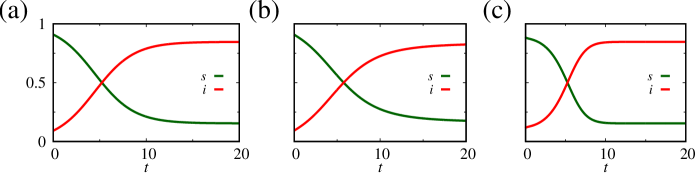
Figure 7: Numerical solutions for $s$ (green line) and $i$ (red line). Panel (a) is for the standard case, the panel (b) is for the fractional case, with $\alpha=0.9$, and the panel (c) for fractal case with $\sigma_{1}=1.9$, $a_{2}=0.82$, and $\sigma_{2}=0.1$. We consider $\beta=204.4$, $\gamma=31.39$, $R_{0}=6.5$, and $i_{0}=0.0912$.

V Conclusions

In this work, we considered the SIS model without demographic characteristics and analysed the extensions described by the substitution of integer operators by non-integer (fractional and fractal). We obtained analytical solutions for the standard (i.e., integer order) and the fractal case. Regarding the fractional situation, we studied the numerical solutions.

Considering these three formulations, we investigated real data from Brazilian syphilis. From 2011 to 2021, our simulations show a basic reproduction number equal to 6.5. We calculated the correlation coefficient between the experimental and theoretical points, namely $r$, to measure the best fit. For the standard case, we obtained $r=0.99$. This formulation adjusts the real data with a good approximation. However, after a specific time (2016), the points follow a different trajectory than the predicted by the model. To adjust these points, we first hypothesise the fit by fractional derivatives due to the increase in the degree of freedom. Our results showed a slowdown in the infected curve, which followed an opposite behaviour compared with points after $t=2017$. The $r$ increases when the fractional order ($\alpha$) tends to the unity, i.e., recovering the standard case. In this situation, it was not possible to improve the fit. The third consideration was the replacement of integer operators with fractal operators. In this case, we constructed a curve of $r$ as a function of $\alpha$. The curve has a maximum point in $\alpha=0.9673$. Therefore, the $r$ value is improved when fractal derivatives are considered. In this case, we obtain $r=0.99028$. Looking at the data behaviour, we observed a different increase in the years 2016 and 2017. In light of this characteristic, we hypothesised that the curve is dominated by one fractal order in a specific range of time and by another fractal order after this time. In this way, we considered two different fractal orders, and our hypothesis was confirmed. We obtain a correlation coefficient equal to 0.998. The fractal model with two orders described the data set with more accuracy than the other considered approaches. This result remains valid when uncertainty, a type of random noise, is added in the data set.

The fractional and fractal operators are a simple way of extending the standard approach and incorporating different effects such as memory effects, long-range correlations, etc. These effects may be related to the relaxation processes present in the system, which deviates from Debye’s case, characterised by exponential relaxations. The non-Debye’s cases present a different behaviour, such as power-law, stretched exponential, mixing between these behaviours, among others. Thus, extending standard operators to fractional or fractal operators is a possibility of capturing these behaviours, which are unsuitable for the usual approaches. Our results show that the fractal formulation describes the data with great accuracy. Comparing our results to the other work Silva2022 , employing geo-processing techniques, we conclude that in addition to the simplicity of the fractal model, it describes the data with a very well accuracy. Models considering more sophisticated statistical analysis and machine learning techniques are found in Refs. Teixeira2023 ; Cervantes2020 ; Zhu2022 . In addition, our model describes the data with great accuracy in the range from 2011 to 2021. In 2022, there is a decrease in the syphilis cases, which is predicted only by the fractional formulation. Data of 2023 are not available from official agencies, however, some brazilian regions report an increase, which is in agreement with our model.

DATA AVAILABILITY

The data that supports the findings of this study are available within the article.

References

References

- (1) W. O. Kermack, A. G. McKendrick, A contribution to the mathematical theory of epidemics, Proc. R. Soc. Lond. A 115 (1927) 700–721.
- (2) M. J. Keeling, P. Rohani, Modeling Infectious Diseases in Humans and Animals, 1st Edition, Princeton University Press, Princeton, 2008.
- (3) O. N. Bjørnstad, Epidemics: Models and Data using R, 1st Edition, Springer Cham, 2018.
- (4) A. Batista, S. de Souza, K. Iarosz, A. de Almeida, J. S. Jr., E. Gabrick, M. Mugnaine, G. dos Santos, I. Caldas, Simulation of deterministic compartmental models for infectious diseases dynamics, Rev. Bras. Ensino Fís. 43 (2021) e20210171.
- (5) L. Allen, Some discrete-time si, sir, and sis epidemic models, Math. Biosc. 124 (1994) 83–105.
- (6) A. Gray, D. Greenhalgh, L. Hu, X. Mao, J. Pan, A stochastic differential equation sis epidemic model, SIAM J. Appl. Math. 71 (2011) 876–902.
- (7) I. Cooper, A. Mondal, C. G. Antonopoulos, A sir model assumption for the spread of covid-19 in different communities, Chaos, Solitons and Fractals 139 (2020) 110057.
- (8) M. Aguiar, B. Kooi, N. Stollenwerk, Epidemiology of dengue fever: A model with temporary cross-immunity and possible secondary infection shows bifurcations and chaotic behaviour in wide parameter regions, Math. Model. Nat. Phenom. 3 (2008) 48–70.
- (9) E. L. Brugnago, R. M. da Silva, C. Manchein, M. W. Beim, How relevant is the decision of containment measures against COVID-19 applied ahead of time?, Chaos, Solitons and Fractals 140 (2020) 110164.
- (10) M. Mugnaine, E. C. Gabrick, P. R. Protachevicz, K. C. Iarosz, S. L. T. de Souza, A. C. L. Almeida, A. M. Batista, I. L. Caldas, J. D. S. Jr., R. L. Viana, Control attenuation and temporary immunity in a cellular automata seir epidemic model, Chaos, Solitons and Fractals 155 (2022) 111784.
- (11) H. W. Hethcote, The mathematics of infectious diseases, SIAM Review 42 (2000) 599–653.
- (12) A. Lajmanovich, J. Yorke, A deterministic model for gonorrhea in a nonhomogeneous population, Math. Biosc. 28 (1976) 221–236.
- (13) C. Manchein, E. L. Brugnago, R. M. da Silva, C. F. O. Mendes, M. W. Beims, Strong correlations between power-law growth of COVID-19 in four continents and the inefficiency of soft quarantine strategies, Chaos 30 (2020) 041102.
- (14) N. Dalal, D. Greenhalgh, X. Mao, A stochastic model for internal HIV dynamics, J. Math. Anal. Appl. 341 (2008) 1084–1101.
- (15) J. Dushoff, J. B. Plotkin, S. A. Levin, D. J. D. Earn, Dynamical resonance can account for seasonality of influenza epidemics, PNAS 101 (2004) 16915–16916.
- (16) M. Aguiar, N. Stollenwerk, B. W. Kooi, Torus bifurcations, isolas and chaotic attractors in a simple dengue fever model with ade and temporary cross immunity, Int. J. of Comp. Math. 86 (2009) 1867–1877.
- (17) M. Amaku, D. T. Covas, F. A. B. Coutinho, R. S. A. Neto, C. Struchiner, A. Wilder-Smith, E. Massad, Modelling the test, trace and quarantine strategy to control the COVID-19 epidemic in the state of São Paulo, Brazil, Inf. Disease Modelling 6 (2021) 46–55.
- (18) S. V. Scarpino, G. Petri, On the predictability of infectious disease outbreaks, Nat. Comm. 10 (2019).
- (19) L. F. Olsen, W. M. Schaffer, Chaos versus noisy periodicity: alternative hypotheses for childhood epidemics, Science 249 (1990) 499–504.
- (20) M. Keeling, B. Grenfell, Stochastic dynamics and a power law for measles variability, Phil. Trans. R. Soc. Lond. B 354 (1999) 769–776.
- (21) S. Altizer, A. Dobson, P. Hosseini, P. Hudson, M. Pascual, P. Rohani, Seasonality and the dynamics of infectious diseases, Eco. Letters 9 (2006) 467–484.
- (22) J. A. Galvis, C. A. Corzo, J. M. Prada, G. Machado, Modeling between-farm transmission dynamics of porcine epidemic diarrhea virus: Characterizing the dominant transmission routes, Prev. Vet. Med. 208 (2022) 105759.
- (23) G. Machado, T. Farthing, M. Andraud, F. Lopes, C. Lanzas, Modelling the role of mortality-based response triggers on the effectiveness of african swine fever control strategies, Trans. and Emer. Diseases 69 (2022) e532–e546.
- (24) O. N. Bjornstad, K. Shea, M. Krzywinski, N. Altman, The SEIRS model for infectious disease dynamics, Nat. Meth. 17 (2020) 557–558.
- (25) K. Shea, O. N. Bjornstad, M. Krzywinski, N. Altman, Uncertainty and the management of epidemics, Nat. Meth. 17 (2020) 867–868.
- (26) O. N. Bjornstad, K. Shea, M. Krzywinski, N. Altman, Modeling infectious epidemics, Nat. Meth. 17 (2020) 455–456.
- (27) E. C. Gabrick, P. R. Protachevicz, A. M. Batista, K. C. Iarosz, S. L. T. de Souza, A. C. L. Almeida, J. D. S. Jr., M. Mugnaine, I. L. Caldas, Effect of two vaccine doses in the seir epidemic model using a stochastic cellular automaton, Phys. A 597 (2022) 127258.
- (28) M. Aguiar, S. Ballesteros, B. W. Kooi, N. Stollenwerk, The role of seasonality and import in a minimalistic multi-strain dengue model capturing differences between primary and secondary infections: complex dynamics and its implications for data analysis, J. of Theor. Bio. 289 (2011) 181–196.
- (29) E. C. Gabrick, E. Sayari, P. R. Protachevicz, J. D. S. Jr., K. C. Iarosz, S. L. T. de Souza, A. C. L. Almeida, R. L. Viana, I. L. Caldas, A. M. Batista, Unpredictability in seasonal infectious diseases spread, Chaos, Solitons and Fractals 166 (2023) 113001.
- (30) S. Ansari, M. Anvari, O. Pfeffer, N. Molkenthin, M. R. Moosavi, F. Hellmann, J. Heitzis, J. Kurths, Moving the epidemic tipping point through topologically targeted social distancing, Eur. Phys. J. Spec. Top. 230 (2021) 3273–3280.
- (31) Z. G. Guo, L. P. Song, G. Q. Sun, C. Li, Z. Jin, Pattern dynamics of an sis epidemic model with nonlocal delay, Int. J. of Bif. and Chaos 29 (2019) 1950027.
- (32) R. M. Anderson, R. M. May, Infectious diseases of humans: Dynamics and control, Oxford University Press, Oxford, 1991.
- (33) H. El-Saka, The fractional-order sis epidemic model with variable population size, J. of the Egy. Math. Soc. 22 (2014) 50–54.
- (34) Z. Dian, Y. Sun, G. Zhang, Y. Xu, X. Fan, X. Yang, Q. Pan, M. Peppelenbosch, Z. Miao, Rotavirus-related systemic diseases: clinical manifestation, evidence and pathogenesis, Crit. Rev. in Micro. 47 (2021) 580–595.
- (35) W. Lynn, S. Lightman, Syphilis and hiv: a dangerous combination, The Lancet Inf. Diseases 4 (2004) 456–466.
- (36) M. Ghosh, P. Chandra, P. Sinha, J. Shukla, Modelling the spread of bacterial infectious disease with environmental effect in a logistically growing human population, Nonlinear Anal.: Real World Appl. 7 (2006) 1468–1218.
- (37) X. Feng, L. Liu, S. Tang, X. Huo, Stability and bifurcation analysis of a two-patch sis model on nosocomial infections, Appl. Math. Letters 102 (2020) 106097.
- (38) D. Pang, Y. Xiao, The sis model with diffusion of virus in the environment, Math. Biosc. and Eng. 16 (2019) 2852–2874.
- (39) A. Misra, A. Sharma, J. Shulka, Modeling and analysis of effects of awareness programs by media on the spread of infectious diseases, Math. and Comp. Modelling 53 (2011) 1221–1228.
- (40) X. Wu, X. Zhou, Y. Chen, K. Zhai, R. Sun, G. L. Y. Lin, Y. Li, C. Yang, H. Zou, The impact of covid-19 lockdown on cases of and deaths from aids, gonorrhea, syphilis, hepatitis b, and hepatitis c: Interrupted time series analysis, JMIR Public Health Surveill 9 (2023) e40591.
- (41) H. W. Hethcote, J. A. Yorke, Gonorrhea Transmission Dynamics and Control, 1st Edition, Springer Berlin, Heidelberg, 1984.
- (42) H. W. Hethcote, P. van den Driessche, An SIS epidemic model with variable population size and a delay, J. Math. Biol. 34 (1995) 177–194.
- (43) A. Gray, D. Greenhalgh, X. Mao, J. Pan, The SIS epidemic model with markovian switching, J. Math. Anal. Appl. 394 (2012) 496– 516.
- (44) D. Gao, S. Ruan, An sis patch model with variable transmission coefficients, Math. Biosc. 232 (2011) 110–115.
- (45) X. Sun, R. Chui, Analysis on a diffusive sis epidemic model with saturated incidence rate and linear source in a heterogeneous environment, J. of Math. Anal. and Appl. 490 (2020) 124212.
- (46) J. Ge, C. Lei, Z. Lin, Reproduction numbers and the expanding fronts for a diffusion–advection sis model in heterogeneous time-periodic environment, Nonl. Anal.: Real World Appl. 33 (2017) 100–120.
- (47) R. Cui, Y. Lou, A spatial sis model in advective heterogeneous environments, J. Diff. Eq. 261 (2016) 3305–3343.
- (48) Y. Cai, S. Yan, H. Wang, X. Lian, W. Wang, Spatiotemporal dynamics in a reaction–diffusion epidemic model with a time-delay in transmission, Int. J. of Bif. and Chaos 25 (2015) 1550099.
- (49) Z. Wu, Y. Cai, Z. Wang, W. Wang, Global stability of a fractional order SIS epidemic model, J. of Diff. Eq. 352 (2023) 221–248.
- (50) N. Liu, J. Fang, W. Deng, J. W. Sun, Stability analysis of a fractional-order sis model on complex networks with linear treatment function, Adv. in Diff. Eq. 327 (2019).
- (51) M. Hassouna, A. Ouhadan, E. E. Kinani, On the solution of fractional order SIS epidemic model, Chaos, Solitons and Fractals 117 (2018) 168–174.
- (52) C. Balzotti, M. D’Ovidio, P. Loreti, Fractional sis epidemic models, Fractal Fract. 44 (2020) 4.
- (53) C. Balzotti, M. D’Ovidio, A. C. Lai, P. Loreti, Effects of fractional derivatives with different orders in sis epidemic models, Comp. 9 (2021) 89.
- (54) C. Xia, S. Sun, F. Rao, J. Sun, J. Wang, Z. Chen, SIS model of epidemic spreading on dynamical networks with community, Front. Comput. Sci. China 3 (2009) 361–365.
- (55) S. Abuasad, A. Yildirim, I. Hashim, S. A. A. Karim, J. Gómez-Aguilar, Fractional multi-step differential transformed method for approximating a fractional stochastic SIS epidemic model with imperfect vaccination, Int. J. Environ. Res. Public Health 16 (2019) 973.
- (56) M. T. Hoang, Z. U. A. Zafar, T. K. Q. Ngo, Dynamics and numerical approximations for a fractional-order SIS epidemic model with saturating contact rate, Comp. and Appl. Math. 39 (2020) 227.
- (57) N. Liu, Y. Li, J. Sun, J. Fang, P. Liu, Epidemic dynamics of a fractional-order sis infectious network model, Disc. Dyn. in Nat. and Soc. 2021 (2021) 5518436.
- (58) L. R. Evangelista, E. K. Lenzi, Fractional Diffusion Equations and Anomalous Diffusion, Cambridge University Press, 2018.
- (59) R. Metzler, J. Klafter, The random walk’s guide to anomalous diffusion: A fractional dynamics approach, Phys. Rep. 339 (2000) 1–77.
- (60) L. R. Evangelista, E. K. Lenzi, An Introduction to Anomalous Diffusion and Relaxation, Springer Nature, 2023.
- (61) V. V. Uchaikin, R. T. Sibatov, Fractional Kinetics in Solids: Anomalous Charge Transport in Semiconductors, Dielectrics and Nanosystems, World Scientific Publishing Company, 2012.
- (62) G. Zaslavsky, Chaos, fractional kinetics, and anomalous transport, Phys. Rep. 371 (2002) 461–580.
- (63) E. K. Lenzi, H. V. Ribeiro, M. K. L. L. R. Evangelista, R. L. Magin, Fractional diffusion with geometric constraints: Application to signal decay in magnetic resonance imaging (MRI), Math. 10 (2022) 389.
- (64) R. Magin, H. Karani, S. Wang, Y. Liang, Fractional order complexity model of the diffusion signal decay in MRI, Math. 7 (2019) 348.
- (65) G. Barbero, L. R. Evangelista, E. K. Lenzi, Time-fractional approach to the electrochemical impedance: The displacement current, J. of Electr. Chem. 920 (2022) 116588.
- (66) J. Bisquert, A. Compte, Theory of the electrochemical impedance of anomalous diffusion, J. of Electr. Chem. 499 (2001) 112–120.
- (67) C. N. Angstmann, A. M. Erickson, B. I. Henry, A. V. McGann, J. M. Murray, J. A. Nichols, A general framework for fractional order compartment models, SIAM Review 63 (2021) 375–392.
- (68) C. N. Angstmann, B. I. Henry, A. V. McGann, A fractional-order infectivity SIR model, Phys. A 452 (2016) 86–93.
- (69) N. Sene, SIR epidemic model with mittag–leffler fractional derivative, Chaos, Solitons and Fractals 137 (2020) 109833.
- (70) A. Taghvaei, T. T. Georgiou, L. Norton, A. Tannenbaum, Fractional SIR epidemiological models, Sci. Rep. 10 (2020) 20882.
- (71) R. Almeida, Analysis of a fractional SEIR model with treatment, Appl. Math. Letters 84 (2018) 56–62.
- (72) Z. Ahmad, M. Arif, F. Ali, I. Khan, K. S. Nisar, A report on COVID-19 epidemic in Pakistan using SEIR fractional model, Sci. Rep. 10 (2020) 22268.
- (73) M. Cai, G. E. Karniadakis, C. Li, Fractional SEIR model and data-driven predictions of COVID-19 dynamics of omicron variant, Chaos 32 (2022) 071101.
- (74) L. Li, C. H. Wang, S. F. Wang, M. T. Li, L. Yakob, B. Cazelles, Z. Jin, W. Y. Zhang, Hemorrhagic fever with renal syndrome in China: Mechanisms on two distinct annual peaks and control measures, Int. J. of Biomath. 11 (2018) 1850030.
- (75) M. Arif, P. Kumam, W. Kumam, A. Akgul, T. Sutthibutpong, Analysis of newly developed fractal-fractional derivative with power law kernel for mhd couple stress fluid in channel embedded in a porous medium, Sci. Rep. 11 (2021) 20858.
- (76) F. Brouers, T. J. Al-Musawi, Brouers-sotolongo fractal kinetics versus fractional derivative kinetics: A new strategy to analyze the pollutants sorption kinetics in porous materials, J. of Hazardous Mat. 350 (2018) 162–168.
- (77) W. Chen, Time–space fabric underlying anomalous diffusion, Chaos, Solitons and Fractals 28 (2006) 923–929.
- (78) W. Chen, H. Sun, X. Zhang, D. Korosak, Anomalous diffusion modeling by fractal and fractional derivatives, Comp. and Math. with Appl. 59 (2010) 1754–1758.
- (79) Q. Wang, J. He, Z. Li, Fractional model for heat conduction in polar bear hairs, Therm. Sci. 16 (2012) 339–342.
- (80) J. He, A tutorial review on fractal spacetime and fractional calculus, Int. J. of Theor. Phys. 53 (2014) 3698–3718.
- (81) H. Cheng, The casimir effect for parallel plates in the spacetime with a fractal extra compactified dimension, Int. J. of Theor. Phys. 52 (2013) 3229–3237.
- (82) J. H. He, Fractal calculus and its geometrical explanation, Results in Phys. 10 (2013) 272–276.
- (83) Y. Zhang, D. A. Benson, D. M. Reeves, Time and space nonlocalities underlying fractional-derivative models: Distinction and literature review of field applications, Adv. in Water Res. 32 (2009) 561–581.
-
(84)
Indicadores de Inconsistências de Sífilis nos Municípios Brasileiros, Available on:
http://indicadoressifilis.aids.gov.br - (85) C. Saad-Roy, Z. Shuai, P. van den Driessche, A mathematical model of syphilis transmission in an MSM population, Math. Biosc. 277 (2016) 59–70.
- (86) F. A. Milner, R. Zhao, A new mathematical model of syphilis, Math. Modelling of Nat. Phen. 5 (2010) 96–108.
- (87) E. Iboi, D. Okuonghae, Population dynamics of a mathematical model for syphilis, Appl. Math. Modelling 40 (2016) 3573–3590.
- (88) Panorama do Censo 2022 - IBGE. Available on: https://censo2022.ibge.gov.br/panorama/ Accessed on: 03-Jul.-2023.
-
(89)
De 2010 a 2022, população brasileira cresce 6,5% e chega a 203,1 milhões. Available on:
https://agenciadenoticias.ibge.gov.br/agencia-noticias/2012-agencia-de-noticias/noticias/37237-de-2010-a-2022-populacao-brasileira-cresce-6-5-e-chega-a-203-1-milhoes - (90) K. Diethelm, N. Ford, A. Freed, Y. Luchko, Algorithms for the fractional calculus: A selection of numerical methods, Comput. Methods Appl. Mech. Engrg 194 (2005) 743–773.
- (91) I. A. Moneim, D. Greenhalgh, Use of a periodic vaccination strategy to control the spread of epidemics with seasonally varying contact rate, Math. Biosc. and Eng. 2(3) (2005) 591-611.
- (92) J. K. Hale, Ordinary Differential Equations, Wiley, New York, 1969.
- (93) S. Gao, L. Chen, Z. Teng, Analysis of an SEIRS epidemic model with time delays and pulse vaccination, Rocky Moun. Jour. of Math. 38(5) (2008) 1385-1402.
- (94) S. Gao, Y. Liu, J. J. Nieto, H. Andrade, Seasonality and mixed vaccination strategy in an epidemic model with vertical transmission, Math. and Comp. in Sim. 81 (2011) 1855-1868.
- (95) T. V. Elzhov, K. M. Mullen, A. N. Spiess, B. Bolker, min-pack.lm: R interface to the levenberg-marquardt nonlinear least-squares algorithm found in minpack, plus support for bounds. r package version 1.2-1. 2020. Available on: https://CRAN.R-project.org/package=minpack.lm
- (96) A. A. O. Silva, L. M. Leony, W. V. de Souza, N. E. M. Freitas, R. T. Daltro, E. F. Santos, L. C. M. Vasconcelos, M. F. R. Grassi, C. G. Regis-Silva, F. L. N. Santos, Spatiotemporal distribution analysis of syphilis in Brazil: Cases of congenital and syphilis in pregnant women from 2001–2017, Plos One 17(10) (2022) e0275731.
- (97) I. V. Teixeira, M. T. S. Leite, F. L. M. Melo, E. S. Rocha, S. Sadok, A. S. P. C. Carrarine, M. Santana, C. P. Rodrigues, A. M. L. Oliveira, K. V. Gadelha, C. M. de Morais, J. Kelner, P. T. Endo, Predicting congenital syphilis cases: A performance evaluation of different machine learning models, Plos One 18(6) (2023) e0276150.
- (98) G. Ibáñez-Cervantes, G. León-García, C. Vargas-De-León, G. Castro-Escarpulli, C. Bandala, O. Sosa-Hernández, J. Mancilla-Ramírez, A. Rojas-Bernabé, M. A. Cureño-Díaz, E. M. Durán-Manuel, C. Cruz-Cruz, J.C. Bravata-Alcántara, D. Juárez-Ascencio, J. M. Bello-López, Epidemiological behavior and current forecast of syphilis in Mexico: increase in male population, Public Health 185 (2020) 386-393.
- (99) Z. Zhu, X. Zhu, Y. Zhan, L. Gu, L. Chen, X. Li, Development and comparison of predictive models for sexually transmitted diseases—AIDS, gonorrhea, and syphilis in China, 2011–2021, Front. Public Health 10 (2022) 966813.