Meta Distribution of Partial-NOMA

Abstract

This work studies the meta distribution (MD) in a two-user partial non-orthogonal multiple access (pNOMA) network. Compared to NOMA where users fully share a resource-element, pNOMA allows sharing only a fraction $\alpha$ of the resource-element. The MD is computed via moment-matching using the first two moments where reduced integral expressions are derived. Accurate approximates are also proposed for the $b{\rm th}$ moment for mathematical tractability. We show that in terms of percentile-performance of links, pNOMA only outperforms NOMA when $\alpha$ is small. Additionally, pNOMA improves the percentile-performance of the weak-user more than the strong-user highlighting its role in improving fairness.

Index Terms: Non-orthogonal multiple access (NOMA), stochastic geometry, meta distribution.

I Introduction

While non-orthogonal multiple access (NOMA) enables a complete sharing of the resource element (RE) by multiple user equipment (UE) to improve throughput, the introduced intracell interference (IaCI) deteriorates the UE coverage. On the contrary, orthogonal multiple access (OMA) has no IaCI, which results in superior coverage, but no spectrum reuse can be applied, which hinders the throughput. Therefore, partial non-orthogonal multiple access (pNOMA) is introduced as a compromise between OMA and NOMA [1]. In contrast to NOMA, UEs in pNOMA share only a fraction $\alpha$ of the RE, which allows spectrum reuse while limiting the IaCI encountered by UEs. In [1], partial sharing of an RE by two users is accomplished by having the two signals overlap only with a fraction of each other in the frequency domain while having complete access to the entire time slot. The partial overlap in the frequency domain allows using matched filtering at the receiver side to further suppress the interference encountered by the UEs, resulting in improved coverage. The matched filtering also enables devising a new decoding technique referred to as flexible successive interference cancellation (FSIC). Using matched filtering in conjunction with FSIC allows pNOMA to outperform NOMA in terms of throughput [1].

Stochastic geometry provides a unified mathematical paradigm for modeling large wireless networks and characterizing their operation while taking into account the experienced intercell interference (ICI) [2, 3]. Research on NOMA [4, 5, 6, 7, 8, 9, 10, 11] and pNOMA [1] have used these tools to analyze networks that encounter both IaCI and ICI. Stochastic geometry-based studies of networks often focus on the spatial averages of performance metrics, the most frequent being the averaged spatial coverage probability (SCP), which averages performance overall fading, activity, and network realizations. However, the actual performance distribution of the majority of the links may not necessarily be close to the SCP. Spatial averages thus do not reveal information about the percentile performance of links that the network operators would be interested in as these reveal the quality of service that the network can offer. It is thus pertinent to study the percentile performance of UEs, where the fading and activity change while the network realization is kept constant. The coverage probability given a fixed network realization is defined as the conditional coverage probability (CCP) [12]. The complementary cumulative distribution function (CCDF) of the CCP, denoted as the meta distribution (MD), reveals the percentile performance across an arbitrary network realization. Since the MD can only be obtained numerically using the Gil-Pelaez theorem, the beta distribution using moment matching of the first two moments of the CCP was proposed as an accurate approximation of the MD [12]. Works such as [9, 10, 11], have studied the MD for NOMA UEsusing this approach.

The SCP, which is the $1{\rm st}$ moment of the CCP, is studied in [1] for a two-user pNOMA network. In contrast, this work focuses on studying the MD of UEs in such a network to reveal more fine-grained information about the performance of such a setup. We derive integral expressions for the $b{\rm th}$ moment of the CCP in a pNOMA network. For the first two moments, which are required to approximate the MD via moment matching, we are able to reduce the integrations required. We also propose accurate approximations for the $b{\rm th}$ moment of the CCP to further simplify the integral calculation and reveal performance trends. Using the exact and approximate moments of the CCP, we compute the MD. This reveals fine-grained information such as the 5%-user performance, which is the reliability that 95% of the UEs can achieve. Our results highlight the superiority of the percentile performance of pNOMA over traditional NOMA in the low $\alpha$ regime. Further, we show that pNOMA improves the performance of the weak UE more, highlighting its role in improving fairness.

Notation: We denote vectors using bold text, $\|\textbf{z}\|$ is used to denote the Euclidean norm of the vector z and $b(\textbf{z},R)$ denotes a ball centered at z with radius $R$. The indicator function, denoted as $\mathbbm{1}_{A}$ has value $1$ when event $A$ occurs and is $0$ otherwise. We use $\psi(x)=\mathrm{sin}(\pi x)/(\pi x)$ when $x\neq 0$, and $\psi(x)=1$ when $x=0$. $\mathbb{E}[\cdot]$ is the expectation and the probability of $A$ is denoted as $\mathbb{P}(A)$.

II System Model and Assumptions

II-A Network Model

We consider a downlink cellular network where the base stations (BSs) are distributed according to a homogeneous Poisson point process (PPP) $\Phi$ with intensity $\lambda$. As a large network is being studied, we assume an interference-limited regime. A BS serves two UEs in each RE via pNOMA using a total power budget of $P=1$. Note that, for simplicity, we do not study pNOMA for more than two UEs sharing a RE as such a setup complicates the analysis without providing additional insights. To the network, we add a BS at the origin o, which under expectation over $\Phi$, becomes the typical BS serving UEs in the typical cell. We study the performance of the typical cell over one RE. As $\Phi$ does not include the BS at o, the set of interfering BSs for the UEs in the typical cell is denoted by $\Phi$. The distance between the typical BS at o and its nearest neighboring BS is denoted by $\rho$. Since $\Phi$ is a PPP, the probability density function (PDF) of $\rho$ is $f_{\rho}(x)=2\pi\lambda xe^{-\pi\lambda x^{2}}$, $x\geq 0$.

Consider a disk around the BS at o with radius $\rho/2$, i.e., $b(\textbf{o},\rho/2)$, this is referred to as the in-disk [4, 1, 9]. The in-disk is the largest disk centered at a BS that fits inside its Voronoi cell. Two pNOMA UEs are distributed uniformly and independently at random in the in-disk $b(\textbf{o},\rho/2)$ of the BS at o. The rationale behind using such a model where UEs are not too far from the serving BS in setups where each UE does not have an individual dedicated RE was shown in [9]. A Rayleigh fading environment is assumed where the fading coefficients are independent and identically distributed (iid) with a unit-mean exponential distribution. A power-law path-loss model is considered where the signal decays at the rate $r^{-\eta}$ with distance $r$, $\eta>2$ denotes the path-loss exponent and $\frac{2}{\eta}\triangleq\delta$. Fixed-rate transmissions are used by the BSs.

II-B pNOMA Model

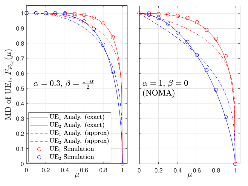
Figure 1: MD vs. $\mu$ using $\theta_{1}=1$ dB, $\theta_{2}=0.5$ dB, and $P_{1}=1/3$.

A BS serves two UEs in each RE via pNOMA by multiplexing the signals for each UE with different power levels using the total power $P$. The RE is split into three regions [1, Fig. 1], $\mathfrak{R}_{1}$, $\mathfrak{R}_{2}$ and $\mathfrak{R}_{3}$, where $\mathfrak{R}_{2}$ is shared by the two UEs. The fraction of the bandwidth (BW) in $\mathfrak{R}_{2}$ is $\alpha$; thus, the UEs have full access to the time slot while they share an overlap $\alpha$ of the frequency. We refer to the fraction of the BW in region $\mathfrak{R}_{1}$, accessible to only $\text{\lx@glossaries@gls@link{acronym}{ue}{\leavevmode UE}}_{1}$, by $\beta$, where $0\leq\beta\leq 1-\alpha$. The remaining fraction of the BW, $1-\alpha-\beta$, in region $\mathfrak{R}_{3}$, is available solely to $\text{\lx@glossaries@gls@link{acronym}{ue}{\leavevmode UE}}_{2}$. Thus, the total fraction of the BW available to $\text{\lx@glossaries@gls@link{acronym}{ue}{\leavevmode UE}}_{1}$ ($\text{\lx@glossaries@gls@link{acronym}{ue}{\leavevmode UE}}_{2}$) is $\text{BW}_{1}=\alpha+\beta$ ($\text{BW}_{2}=1-\beta$).

An overlap in the frequency domain allows implementing filtering at the receiver side to further suppress interference. A matched filter that has a Fourier transform equal to the complex conjugate of the Fourier transform of the transmitted signal is used [1, 13]. In this work, we adopt square pulse shaping for transmissions of both UEs. A message that goes through receive filtering and has an $\alpha$-overlap with the message of the UE of interest will be scaled by an effective interference factor $0\leq\mathcal{I}(\alpha,\beta)\leq 1$. From [1], the effective interference factor as a function of $\beta$ and the overlap $\alpha$ is calculated as

$$\mathcal{I}(\alpha,\beta)\!=\!\left(\!\int\nolimits_{\beta}^{\beta+\alpha}\!\frac{1}{E_{1}E_{2}}\psi\!\left(\!\frac{f-f_{a}}{0.5\text{BW}_{1}}\!\right)\!\psi\!\left(\frac{f-f_{b}}{0.5\text{BW}_{2}}\!\right)df\!\right)^{{2}}$$ (1)

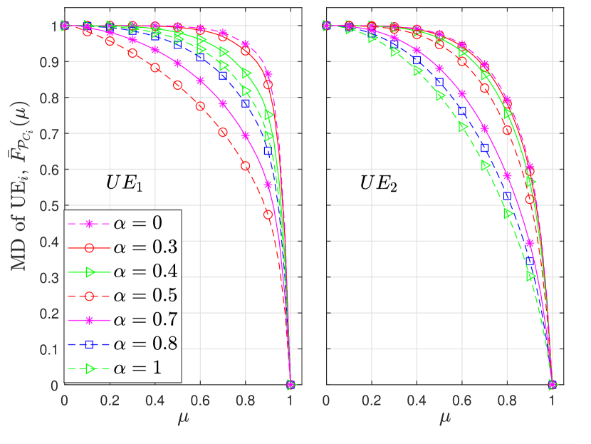
Figure 2: MD vs. $\mu$, $P_{1}\!\!=\!\!1/3$, $\theta_{1}\!=\!1$ dB, $\theta_{2}=0.5$ dB and $\beta=\frac{1-\alpha}{2}$.

where the center frequency of $\text{\lx@glossaries@gls@link{acronym}{ue}{\leavevmode UE}}_{1}$ is $f_{a}=\frac{\alpha+\beta}{2}$ and $\text{\lx@glossaries@gls@link{acronym}{ue}{\leavevmode UE}}_{2}$ is $f_{b}=\frac{1+\beta}{2}$. The factors $E_{i}$ for $i\in\{1,2\}$ are used to scale the energy to $1$ and are calculated as $E_{i}^{2}=\int_{-\text{BW}_{i}/2}^{\text{BW}_{i}/2}\psi^{2}\left(\frac{2f}{\text{BW}_{i}}\right)df$. Note that $\mathcal{I}(\alpha,\beta)$ increases monotonically with $\alpha$ and is $1$ ($0$) when $\alpha=1$ ($\alpha=0$) [1, Fig. 2]. As $0\leq\mathcal{I}(\alpha,\beta)\leq 1$, matched filtering results in suppression of the interference from the other UE partially sharing the RE. Since any message that has an $\alpha$-overlap with the UE of interest is scaled by $\mathcal{I}(\alpha,\beta)$, not only does matched filtering suppress IaCI, but also reduces ICI.

We order the UEs based on the link distance $R$ between the typical BS at o and its UEs that are uniformly distributed in the in-disk with radius $\rho$. This is equivalent to ordering based on the decreasing received mean signal power, i.e., $R^{-\eta}$. Thus, we refer to the strong (weak) UE as $\text{\lx@glossaries@gls@link{acronym}{ue}{\leavevmode UE}}_{1}$ ($\text{\lx@glossaries@gls@link{acronym}{ue}{\leavevmode UE}}_{2}$). As the order of the UEs is known at the BS, we use ordered statistics for the PDF of $R_{i}$ [14],

$$f_{R_{i}\mid\rho}(r\mid\rho)=16r\rho^{-2}\left(4r^{2}\rho^{-2}\right)^{i-1}\left(1-4r^{2}\rho^{-2}\right)^{2-i}.$$ (2)

While NOMA uses successive interference cancellation (SIC) for decoding, after matched filtering in pNOMA, the message of $\mathrm{\lx@glossaries@gls@link{acronym}{ue}{\leavevmode UE}}_{2}$ scaled by $\mathcal{I}(\alpha,\beta)$ can be too weak for $\mathrm{\lx@glossaries@gls@link{acronym}{ue}{\leavevmode UE}}_{1}$ to decode; FSIC was thus introduced in [1] to combat this problem.

The power allocated to $\text{\lx@glossaries@gls@link{acronym}{ue}{\leavevmode UE}}_{1}$ ($\text{\lx@glossaries@gls@link{acronym}{ue}{\leavevmode UE}}_{2}$) is denoted by $P_{1}$ ($P_{2}$) and $P_{1}+P_{2}=1$. For fixed rate transmission, the rate of $\text{\lx@glossaries@gls@link{acronym}{ue}{\leavevmode UE}}_{i}$, $i\in\{1,2\}$, is $\log(1+\theta_{i})$. Accordingly, to decode the message of $\text{\lx@glossaries@gls@link{acronym}{ue}{\leavevmode UE}}_{i}$, the signal to interference ratio (SIR) needs to exceed $\theta_{i}$.The throughput of $\text{\lx@glossaries@gls@link{acronym}{ue}{\leavevmode UE}}_{i}$, $i\in\{1,2\}$ is defined as $\mathcal{T}_{i}=\text{BW}_{i}\;\mathbb{P}(C_{i})\;\log(1+\theta_{i}),$ where $C_{i}$ is the event that $\text{\lx@glossaries@gls@link{acronym}{ue}{\leavevmode UE}}_{i}$ is in coverage. The sum throughput of the typical cell is thus $\mathcal{T}_{1}+\mathcal{T}_{2}$. As $\text{BW}_{i}$ is a function of both $\alpha$ and $\beta$, the resources to be allocated in a pNOMA setup for a given $\alpha$ are $P_{1}=(1-P_{2})$, $\theta_{1}$, $\theta_{2}$ and $\beta$.

II-C SIRs Associated With pNOMA and Coverage Events

Because pNOMA uses FSIC, there are multiple SIRs of interest. For the two-user downlink pNOMA we require ${\rm SIR}_{j}^{i}$, the SIR for decoding the $j{\rm th}$ message at $\text{\lx@glossaries@gls@link{acronym}{ue}{\leavevmode UE}}_{i}$ where $i\leq j$ and the messages of all UEs weaker than $\text{\lx@glossaries@gls@link{acronym}{ue}{\leavevmode UE}}_{j}$ have been removed while the messages of all UEs stronger than $\text{\lx@glossaries@gls@link{acronym}{ue}{\leavevmode UE}}_{j}$ are treated as noise. In particular,

$$\mathrm{SIR}_{2}^{2}=\left(h_{2}R_{2}^{-\eta}P_{2}\right)/\left(h_{2}R_{2}^{-\eta}P_{1}\mathcal{I}(\alpha,\beta)+\tilde{I}_{2}^{\mathrm{\o}}\right)$$ (3)

$$\mathrm{SIR}_{2}^{1}=\left(h_{1}R_{1}^{-\eta}P_{2}\mathcal{I}(\alpha,\beta)\right)/\left(h_{1}R_{1}^{-\eta}P_{1}+\tilde{I}_{1}^{\mathrm{\o}}\right)$$ (4)

$$\mathrm{SIR}_{1}^{1}=\left(h_{1}R_{1}^{-\eta}P_{1}\right)/\tilde{I}_{1}^{\mathrm{\o}}$$ (5)

where $\tilde{I}^{\rm\o}_{i}$ is the ICI experienced at UE_i, $\tilde{I}^{\rm\o}_{i}=\left(P_{i}+(1-P_{i})\mathcal{I}(\alpha,\beta)\right)\sum_{\textbf{x}\in\Phi}g_{\textbf{y}_{i}}{\|\textbf{y}_{i}\|}^{-\eta}$, where $\textbf{y}_{i}=\textbf{x}-\textbf{u}_{i}$ and $\textbf{u}_{i}$ is the location of $\text{\lx@glossaries@gls@link{acronym}{ue}{\leavevmode UE}}_{i}$. The fading coefficient from the serving BS (interfering BS) located at o (x) to $\text{\lx@glossaries@gls@link{acronym}{ue}{\leavevmode UE}}_{i}$ is $h_{i}$ ($g_{\textbf{y}_{i}}$). The ICI scaled to unit transmission power by each interferer is defined as $I^{\rm\o}_{i}$, hence, $\tilde{I}^{\rm\o}_{i}=\left(P_{i}+(1-P_{i})\mathcal{I}(\alpha,\beta)\right)I^{\rm\o}_{i}$. Because $\left(P_{i}+(1-P_{i})\mathcal{I}(\alpha,\beta)\right)\!\!\leq\!\!1$, ICI in pNOMA is lower than its traditional counterparts. Additionally, since the network model conditions an interferer to exist at a distance $\rho$ from the typical BS at o, we can rewrite $I^{\rm\o}_{i}$ as

$$I_{i}^{\mathrm{\o}}=\sum_{\mathbf{x}\in\Phi,\|\mathbf{x}\|>\rho}g_{\mathbf{y}_{i}}{\|\mathbf{y}_{i}\|}^{-\eta}+\sum_{\mathbf{x}\in\Phi,\|\mathbf{x}\|=\rho}g_{\mathbf{y}_{i}}{\|\mathbf{y}_{i}\|}^{-\eta}.$$ (6)

Note that as there is no interfering BS inside $b(\textbf{o},\rho)$, the nearest interfering BS from $\text{\lx@glossaries@gls@link{acronym}{ue}{\leavevmode UE}}_{i}$ is at least $\rho-R_{i}$ away. As $\rho-R_{i}>R_{i}$, the in-disk model offers a larger guard zone than the usual guard zone of link distance for UEs in a downlink Poisson network [4].

While ${\rm SIR}_{1}^{1}$ is associated with $\text{\lx@glossaries@gls@link{acronym}{ue}{\leavevmode UE}}_{1}$ decoding its message after decoding and cancelling the message of $\text{\lx@glossaries@gls@link{acronym}{ue}{\leavevmode UE}}_{2}$, FSIC also allows $\text{\lx@glossaries@gls@link{acronym}{ue}{\leavevmode UE}}_{1}$ to decode its own message while treating the message of $\text{\lx@glossaries@gls@link{acronym}{ue}{\leavevmode UE}}_{2}$ as noise. The SIR associated with $\text{\lx@glossaries@gls@link{acronym}{ue}{\leavevmode UE}}_{1}$ for decoding its own message when the message of $\text{\lx@glossaries@gls@link{acronym}{ue}{\leavevmode UE}}_{2}$ has not been canceled is

$$\mathrm{\widetilde{SIR}}_{1}^{1}=\left(h_{1}R_{1}^{-\eta}P_{1}\right)/\left(h_{1}R_{1}^{-\eta}P_{2}\mathcal{I}(\alpha,\beta)+\tilde{I}_{1}^{\mathrm{\o}}\right).$$ (7)

As FSIC decoding for $\text{\lx@glossaries@gls@link{acronym}{ue}{\leavevmode UE}}_{2}$ involves decoding its own message while treating the interference from the message of $\text{\lx@glossaries@gls@link{acronym}{ue}{\leavevmode UE}}_{1}$ as noise, the event of successful decoding at $\text{\lx@glossaries@gls@link{acronym}{ue}{\leavevmode UE}}_{2}$ is defined as

$$C_{2}=\left\{{\rm SIR}_{2}^{2}>\theta_{2}\right\}=\left\{h_{2}>R_{2}^{\eta}\tilde{I}^{\rm\o}_{2}\bar{M}_{2}\right\},$$ (8)

$$\bar{M}_{2}={\theta_{2}}/\left(\>{P_{2}-\theta_{2}P_{1}\mathcal{I}(\alpha,\beta)}\>\right).$$ (9)

FSIC decoding for $\text{\lx@glossaries@gls@link{acronym}{ue}{\leavevmode UE}}_{1}$, on the other hand, is the joint event as described in Section II-B. The event of successful decoding at $\text{\lx@glossaries@gls@link{acronym}{ue}{\leavevmode UE}}_{1}$ is thus defined as

$$C_{1}=\left\{\left({\rm SIR}_{2}^{1}>\theta_{2}\bigcap{\rm SIR}_{1}^{1}>\theta_{1}\right)\bigcup{\rm\widetilde{SIR}}_{1}^{1}>\theta_{1}\right\}$$

$$=\left\{\!h_{1}\!>\!R_{1}^{\eta}\tilde{I}^{\mathrm{\o}}_{1}M_{1}\bigcup h_{1}>R_{1}^{\eta}\tilde{I}^{\mathrm{\o}}_{1}M_{0}\!\right\}=\left\{\!h_{1}>R_{1}^{\eta}\tilde{I}^{\rm\o}_{1}\bar{M}_{1}\!\right\},$$ (10)

$$\bar{M}_{1}=\min\left\{M_{0},M_{1}\right\}\mathbbm{1}_{\tilde{P}_{1}>0}\mathbbm{1}_{\tilde{P}_{2}^{1}>0}\mathbbm{1}_{P_{1}>0}\\ +M_{0}\mathbbm{1}_{\tilde{P}_{1}>0}\mathbbm{1}_{\tilde{P}_{2}^{1}\leq 0\;\cup P_{1}\leq 0}\;+\;M_{1}\mathbbm{1}_{\tilde{P}_{1}\leq 0}\mathbbm{1}_{\tilde{P}_{2}^{1}>0}\mathbbm{1}_{P_{1}>0}$$ (11)

using $\tilde{P}_{1}=P_{1}-\theta_{1}P_{2}\mathcal{I}(\alpha,\beta)$, $\;\tilde{P}_{2}^{1}=P_{2}\mathcal{I}(\alpha,\beta)-\theta_{2}P_{1}$, $\;M_{0}={\theta_{1}}{/\tilde{P}_{1}}$ and $M_{1}=\max\left\{{\theta_{2}}/{\tilde{P}_{2}^{1}},{\theta_{1}}/{P_{1}}\right\}$.

The event of successful decoding at $\text{\lx@glossaries@gls@link{acronym}{ue}{\leavevmode UE}}_{i}$ is thus of the form $C_{i}=\left\{h_{i}>R_{i}^{\eta}\tilde{I}^{\rm\o}_{i}\bar{M}_{i}\right\}$. Using $\tilde{I}^{\rm\o}_{i}=(P_{i}+(1-P_{i})\mathcal{I}(\alpha,\beta))I^{\rm\o}_{i}$ and $\tilde{M}_{i}=(P_{i}+(1-P_{i})\mathcal{I}(\alpha,\beta))\bar{M}_{i}$, we can rewrite $C_{i}$ as

$$C_{i}=\left\{h_{i}>R_{i}^{\eta}I^{\rm\o}_{i}\tilde{M}_{i}\right\}.$$ (12)

III Analysis of the Meta Distribution

The CCP is defined as the coverage probability given a fixed network realization [12]. For a fixed, yet arbitrary, realization of the network $\mathcal{P}_{C_{i}}$, the CCP of $\text{\lx@glossaries@gls@link{acronym}{ue}{\leavevmode UE}}_{i}$ in a pNOMA network is

$$\mathcal{P}_{C_{i}}\!\overset{\Delta}{=}\mathbb{P}(C_{i}\mid\Phi)\!\overset{(a)}{=}\mathbb{E}_{g_{\mathbf{y}_{i}}}\!\left[\!\ \exp\left(\!-R_{i}^{\eta}\tilde{M}_{i}\sum\nolimits_{\mathbf{x}\in{\Phi}}g_{\mathbf{y}_{i}}{\|\mathbf{y}_{i}\|}^{-\eta}\!\right)\mid\Phi\right]$$

$$\overset{(b)}{=}\prod\nolimits_{\mathbf{x}\in{\Phi}}\left({1+R_{i}^{\eta}\tilde{M}_{i}{\|\mathbf{y}_{i}\|}^{-\eta}}\right)^{-1},$$ (13)

where $(a)$ follows by using the definition of $C_{i}$ in (12) and the cumulative distribution function (CDF) of $h_{i}\sim\exp(1)$. Using the moment generation function (MGF) of the independent random variables $g_{\textbf{y}_{i}}\sim\exp(1)$, $(b)$ is obtained.

The requirement for more fine-grained information on performance leads to the notion of studying the distribution of the CCP. The MD was thus defined as the CCDF of the CCP [12]. The MD for $\text{\lx@glossaries@gls@link{acronym}{ue}{\leavevmode UE}}_{i}$ can be written as: $\bar{F}_{\mathcal{P}_{C_{i}}}(\mu)\stackrel{{\scriptstyle\triangle}}{{=}}\mathbb{P}(\mathcal{P}_{C_{i}}>\mu),\;\;0\leq\mu\leq 1.$

The $b{\rm th}$ moment of the CCP of $\text{\lx@glossaries@gls@link{acronym}{ue}{\leavevmode UE}}_{i}$, by definition, can be calculated using (13) as

$$\mathcal{M}_{i,b}=\mathbb{E}\left[\mathcal{P}_{C_{i}}^{b}\right]=\mathbb{E}\left[\prod\nolimits_{\mathbf{x}\in{\Phi}}\left(1+R_{i}^{\eta}\tilde{M}_{i}{\|\mathbf{y}_{i}\|}^{-\eta}\right)^{-b}\right].$$ (14)

Note that by definition, the SCP of $\text{\lx@glossaries@gls@link{acronym}{ue}{\leavevmode UE}}_{i}$ is the first moment of the CCP of $\text{\lx@glossaries@gls@link{acronym}{ue}{\leavevmode UE}}_{i}$, i.e., $\mathcal{M}_{i,1}$.

Deriving the MD is generally intractable. Therefore, the beta distribution using moment matching was proposed as a very accurate approximation for the MD [12]. This approach only requires the first two moments of the CCP, i.e., $\mathcal{M}_{i,1}$ and $\mathcal{M}_{i,2}$. In particular,

$${\bar{F}_{{\mathcal{P}_{C_{i}}}}(\mu)}\approx 1-\mathcal{I}_{\mu}\left(\beta_{i}\mathcal{M}_{i,1}\left(1-\mathcal{M}_{i,1}\right)^{-1},\beta_{i}\right)$$ (15)

where $\beta_{i}$=$\frac{(\mathcal{M}_{i,1}-\mathcal{M}_{i,2})(1-\mathcal{M}_{i,1})}{\mathcal{M}_{i,2}-\mathcal{M}_{i,1}^{2}}$ and $\mathcal{I}_{\mu}(a,b)=\int_{0}^{\alpha}l^{a-1}(1-l)^{b-1}dl$ is the regularized incomplete beta function.

III-A Exact Moments of the Conditional Coverage Probability

This subsection evaluates the moments of the CCP of $\text{\lx@glossaries@gls@link{acronym}{ue}{\leavevmode UE}}_{i}$.

Lemma 1: The $b{\rm th}$ moment of the CCP of $\text{\lx@glossaries@gls@link{acronym}{ue}{\leavevmode UE}}_{i}$ is

$$\mathcal{M}_{i,b}\approx\mathbb{E}_{\rho,R_{i}}\left[\exp\left(-2\pi\lambda\mathcal{A}_{i,b}\right){\left(1+\tilde{M}_{i}{R_{i}^{\eta}}{\rho^{-\eta}}\right)}^{-b}\right],$$ (16)

$$\mathcal{A}_{i,b}=\int\nolimits_{\rho-R_{i}}^{\infty}\left(1-\left(1+\tilde{M}_{i}{R_{i}^{\eta}}{r^{-\eta}}\right)^{-b}\right)rdr.$$ (17)

Proof: By writing $\mathcal{M}_{i,b}$ according to the definition in (14), and separating the ICI along the lines of (6), we obtain

$$\mathcal{M}_{i,b} \!=\!\mathbb{E}\!\Bigg{[}\!\prod\limits_{\begin{subarray}{c}\textbf{x}\in\Phi\\ {\|\textbf{x}\|}>\rho\end{subarray}}\!\!\left(\!1\!+\!{\tilde{M}_{i}R_{i}^{\eta}}{{\|\textbf{y}_{i}\|}^{-\eta}}\!\right)^{-b}\!\!\prod\limits_{\begin{subarray}{c}\textbf{x}\in\Phi\\ {\|\textbf{x}\|}=\rho\end{subarray}}\!\!\left(\!1\!+\!{\tilde{M}_{i}R_{i}^{\eta}}{{\|\textbf{y}_{i}\|}^{-\eta}}\!\right)^{-b}\!\Bigg{]}$$

$${\stackrel{{\scriptstyle(a)}}{{=}}\mathbb{E}_{\rho,R_{i}}\left[e^{-2\pi\lambda\mathcal{A}_{i,b}}\mathbb{E}_{w}\left[\!{\left(\!1+{\tilde{M}_{i}R_{i}^{\eta}}{{w}^{-\eta}}\!\right)}^{-b}\!\right]\right]}$$

$${\stackrel{{\scriptstyle(b)}}{{\approx}}\mathbb{E}_{\rho,R_{i}}\left[e^{-2\pi\lambda\mathcal{A}_{i,b}}{\left(1+\tilde{M}_{i}{R_{i}^{\eta}}{{\mathbb{E}[w]}^{-\eta}}\right)}^{-b}\right].}$$

Using (6), the second term inside the expectation comes from the nearest interferer from o which is a distance $\rho$ from o, while the first term comes from the other interferers that are located at distances larger than $\rho$ from o. In $(a)$, we arrive at the first term of this expression and (16) using the probability generating functional (PGFL) of the PPP. Note that since the in-disk model allows a larger guard zone, the lower limit on the distance from the nearest interferer, in the inner integral $\mathcal{A}_{i,b}$, is $\rho-R_{i}$. The second term of $(a)$ comes from denoting the distance between $\text{\lx@glossaries@gls@link{acronym}{ue}{\leavevmode UE}}_{i}$ and the BS at distance $\rho$ from o by $w$. For simplicity, in $(b)$ we used the approximate mean of the distance $w$ which was validated as a tight approximation and in (16) $\mathbb{E}[w]\approx\rho$ as the difference between $\mathbb{E}[w]$ and $\rho$ is less than 3.2% [4]. ∎

For general $b$, $\mathcal{M}_{i,b}$ requires a triple integral according to (16). However, for $b\in\{1,2\}$, closed-form expressions for $\mathcal{A}_{i,b}$ in (16) can be obtained, reducing the calculation in (16) by one integral. Note that $\mathcal{M}_{i,1}$ and $\mathcal{M}_{i,2}$ are the two most relevant moments of the CCP of $\text{\lx@glossaries@gls@link{acronym}{ue}{\leavevmode UE}}_{i}$ as they are sufficient to evaluate the MD of $\text{\lx@glossaries@gls@link{acronym}{ue}{\leavevmode UE}}_{i}$.
Corollary 1: The inner integral for calculating the first moment of the CCP, i.e., the SCP, of $\text{\lx@glossaries@gls@link{acronym}{ue}{\leavevmode UE}}_{i}$, $\mathcal{M}_{i,1}$, is

$$\mathcal{A}_{i,1}=\frac{\tilde{M}_{i}R_{i}^{\eta}}{\eta-2}(\rho-R_{i})^{2-\eta}{}_{2}F_{1}\Big{(}1,1\!-\!\delta;2\!-\!\delta;\frac{-\tilde{M}_{i}R_{i}^{\eta}}{(\rho-R_{i})^{\eta}}\Big{)}.$$ (18)

Corollary 2: The inner integral for calculating the second moment of the CCP of $\text{\lx@glossaries@gls@link{acronym}{ue}{\leavevmode UE}}_{i}$, $\mathcal{M}_{i,2}$, is

$$\mathcal{A}_{i,2}=\frac{\tilde{M}_{i}R_{i}^{\eta}}{\eta}\Bigg{(}\frac{2(\rho\!-\!R_{i})^{\eta}+\tilde{M}_{i}R_{i}^{\eta}}{(\rho\!-\!R_{i})^{\eta}+\tilde{M}_{i}R_{i}^{\eta}}(\rho\!-\!R_{i})^{2-\eta}\\ +\frac{(\eta\!-\!2)\tilde{M}_{i}R_{i}^{\eta}}{2(1\!-\!\eta)}(\rho\!-\!R_{i})^{2-2\eta}{}_{2}F_{1}\left(1,2\!-\!\delta;3\!-\!\delta;-\tilde{M}_{i}R_{i}^{\eta}(\rho\!-\!R_{i})^{-\eta}\right)\\ +\frac{4(\rho\!-\!R_{i})^{2-\eta}}{(\eta\!-\!2)}{}_{2}F_{1}\left(1,1\!-\!\delta;2\!-\!\delta;-\tilde{M}_{i}R_{i}^{\eta}(\rho\!-\!R_{i})^{-\eta}\right)\Bigg{)}.$$ (19)

III-B Approximate Moments of the Conditional Coverage Probability

Evaluating the $b{\rm th}$ moment of the CCP of $\text{\lx@glossaries@gls@link{acronym}{ue}{\leavevmode UE}}_{i}$ in Section III-A requires a triple integral for general $b$, and a double integral for $b=1,2$. Therefore, an alternative approach to calculate the moments that is based on the relative distance process (RDP) is used [15]. Since pNOMA deals with ordered link distances, the ordered RDP is used, which for $\text{\lx@glossaries@gls@link{acronym}{ue}{\leavevmode UE}}_{i}$ is defined as: $\mathcal{R}_{i}=\left\{\mathbf{x}\in\Phi:R_{i}\|\mathbf{y}_{i}\|^{-1}\right\}.$

Using the ordered RDP for $\text{\lx@glossaries@gls@link{acronym}{ue}{\leavevmode UE}}_{i}$, we can rewrite the moments of the CCP of $\text{\lx@glossaries@gls@link{acronym}{ue}{\leavevmode UE}}_{i}$ in (14) as

$$\mathcal{M}_{i,b}=\mathbb{E}\left[\prod\nolimits_{z\in{\mathcal{R}_{i}}}\left(1+\tilde{M}_{i}z^{\eta}\right)^{-b}\right].$$ (20)

As (14) is in terms of the PPP $\Phi$, evaluating $\mathcal{M}_{i,b}$ in (16) requires the probability generating functional (PGFL) of the PPP. Accordingly, as $\mathcal{M}_{i,b}$ in (20) is in terms of the RDP $\mathcal{R}_{i}$, the PGFL of $\mathcal{R}_{i}$ is required to evaluate $\mathcal{M}_{i,b}$. Because $R_{i}$ and therefore the RDP $\mathcal{R}_{i}$ are conditioned on $\rho$, the PGFL of $\mathcal{R}_{i}$ is also conditioned on $\rho$.

Lemma 2: The PGFL of the ordered $\mathcal{R}_{i}$ conditioned on $\rho$ is

$$\!\mathcal{G}_{\mathcal{R}_{i}\!\mid\rho}\![f]\!=\!\mathbb{E}_{R_{i}\!\mid\rho}\!\Bigg{[}\!\exp\!\Big{(}\!\!-\!2\pi\!\lambda\!\!\!\int\limits_{\rho\!-\!R_{i}}^{\infty}\!\!\!\left(\!1\!\!-\!\!f\!\left(\!\frac{\!R_{i}}{\!a}\!\right)\!\!\right)\!a\!da\!\Big{)}\!\!\!\prod\limits_{\begin{subarray}{c}\textbf{x}\in\Phi\\ \|\!\textbf{x}\|=\!\rho\end{subarray}}\!\!f\!\left(\!\!\frac{R_{i}}{\|\textbf{y}_{i}\|}\!\!\right)\!\Bigg{]}.$$ (21)

Proof: By definition of the PGFL we have

$$\mathcal{G}_{\mathcal{R}_{i}\mid\rho}[f]\stackrel{{\scriptstyle\triangle}}{{=}}\mathbb{E}\Big{[}\prod\limits_{z\in\mathcal{R}_{i}}f(z)\Big{]}=\mathbb{E}\Big{[}\prod\limits_{{\textbf{x}\in\Phi}}f\left({R_{i}}{\|\textbf{y}_{i}\|^{-1}}\right)\Big{]}.$$

By separating the interferers along the lines of (6) and using the PGFL of the PPP, (21) is obtained. ∎

However, it is infeasible to obtain tractable expressions for the moments of the CCP using (21).Therefore, we propose the use of two approximations to relax the constraints and simplify the calculation of the PGFL of the ordered RDP for $\text{\lx@glossaries@gls@link{acronym}{ue}{\leavevmode UE}}_{i}$. The approximations are:

• A1: The guard zone around the UEs is approximated to be of radius $R_{i}$ (instead of the largest guaranteed radius $\rho-R_{i}>R_{i}$).

• A2: Deconditioning on the BS located a distance $\rho$ from o.

Note that the two approximations have opposing effects on how much ICI is accounted; A1 overestimates it while A2 underestimates it.

Lemma 3: The PGFLs of the ordered RDP for $\text{\lx@glossaries@gls@link{acronym}{ue}{\leavevmode UE}}_{2}$ and $\text{\lx@glossaries@gls@link{acronym}{ue}{\leavevmode UE}}_{1}$, respectively, using approximations A1 and A2 are

$$\widetilde{\mathcal{G}}_{\mathcal{R}_{2}|\rho}[f]\!=\!\frac{32}{\rho^{4}}\frac{\Gamma(2)\!-\!\Gamma\Big{(}2,\frac{\rho^{2}}{2}\pi\lambda\int_{1}^{\infty}\left(\!1\!-\!f(\frac{1}{y})\!\right)ydy\Big{)}}{\Big{(}\!2\pi\lambda\int_{1}^{\infty}\left(\!1\!-\!f(\frac{1}{y})\!\right)ydy\!\Big{)}^{2}}$$ (22)

$$\widetilde{\mathcal{G}}_{\mathcal{R}_{1}|\rho}[f]\!=\!\frac{\Gamma(1)\!-\!\Gamma\!\left(\!1,\frac{\rho^{2}}{2}\!\pi\lambda\int_{1}^{\infty}\!\left(\!1\!-\!f(\frac{1}{y})\!\right)ydy\!\right)\!}{\frac{\rho^{2}}{4}\pi\lambda\int_{1}^{\infty}\left(\!1\!-\!f(\frac{1}{y})\!\right)ydy}\!-\!\widetilde{\mathcal{G}}_{\mathcal{R}_{2}|\rho}[f].$$ (23)

Proof: Along the lines of the proof of Lemma 2, the PGFL of the ordered RDP for $\text{\lx@glossaries@gls@link{acronym}{ue}{\leavevmode UE}}_{i}$ using A1 and A2 is

$$\widetilde{\mathcal{G}}_{\mathcal{R}_{i}\mid\rho}[f]=\mathbb{E}_{R_{i}\mid\rho}\left[\exp\left(-2\pi\lambda\int_{R_{i}}^{\infty}\left(1-f\left({R_{i}}/{a}\right)\right)a\;da\right)\right].$$

Here the second term in (21) has been removed due to A2. Additionally, the lower limit of the integral of the first term in (21) is updated to reflect $R_{i}$, the radius of the guard zone in A1. Using $f_{R_{i}\mid\rho}$ in (2) for $i=2$ and $i=1$ we obtain (22) and (23), respectively. ∎

Lemma 4: The $b{\rm th}$ moments of the CCP for $\text{\lx@glossaries@gls@link{acronym}{ue}{\leavevmode UE}}_{2}$ and $\text{\lx@glossaries@gls@link{acronym}{ue}{\leavevmode UE}}_{1}$, respectively, using approximations A1 and A2 are

$$\widetilde{\mathcal{M}}_{2,b}\!=\!\mathbb{E}_{\rho}\!\left[\!\frac{32}{\rho^{4}}\frac{1\!-\!\Gamma\left(2,\frac{\rho^{2}}{4}\pi\lambda\!\left(\!{}_{2}F_{1}(b,\!-\!\delta;1\!-\!\delta;\!-\tilde{M}_{2})\!-\!1\!\right)\right)}{\left(\pi\lambda\!\left(\!{}_{2}F_{1}(b,-\delta;1\!-\!\delta;-\tilde{M}_{2})-1\!\right)\right)^{2}}\!\right]$$ (24)

$$\widetilde{\mathcal{M}}_{1,b}=\mathbb{E}_{\rho}\Bigg{[}\frac{8}{\rho^{2}}\frac{1-\exp\left(-\frac{\rho^{2}}{4}\pi\lambda\left({}_{2}F_{1}(b,-\delta;1\!-\!\delta;-\tilde{M}_{1})-1\right)\right)}{\pi\lambda\left({}_{2}F_{1}(b,-\delta;1\!-\!\delta;-\tilde{M}_{1})-1\right)}$$

$$-\frac{32}{\rho^{4}}\frac{1-\Gamma\left(2,\frac{\rho^{2}}{4}\pi\lambda\left({}_{2}F_{1}(b,-\delta;1\!-\!\delta;-\tilde{M}_{1})-1\right)\right)}{\left(\pi\lambda\left({}_{2}F_{1}(b,-\delta;1\!-\!\delta;-\tilde{M}_{1})-1\right)\right)^{2}}\Bigg{]}.$$ (25)

Proof: Using the definition in (20), we have

$$\widetilde{\mathcal{M}}_{i,b}=\mathbb{E}_{\rho}\left[\widetilde{\mathcal{G}}_{\mathcal{R}_{i}\mid\rho}[f(z)]\Big{|}_{f(z)=(1+\tilde{M}_{i}z^{\eta})^{-b}}\right].$$

$\widetilde{\mathcal{G}}_{\mathcal{R}_{i}\mid\rho}[f(z)]$ in (23) and (22) for $\text{\lx@glossaries@gls@link{acronym}{ue}{\leavevmode UE}}_{1}$ and $\text{\lx@glossaries@gls@link{acronym}{ue}{\leavevmode UE}}_{2}$, respectively, are then plugged into the equation above. We arrive at (24) and (25) using the following, where (a) is obtained using $z\rightarrow g^{-1}$:

$$\int_{1}^{\infty}\!\left(\!1\!-\!f(z^{-1})\!\right)zdz\Big{|}_{f(z)=(1+\tilde{M}_{i}z^{\eta})^{-b}}$$

$$\!=\!\int_{1}^{\infty}\!\!\left(\!1\!-\!(1\!+\!\tilde{M}_{i}z^{-\eta})^{-b}\!\right)zdz\!\stackrel{{\scriptstyle(a)}}{{=}}\!\frac{{}_{2}F_{1}\left(b,\!-\delta;1\!-\!\delta,\!-\tilde{M}_{i}\right)\!-\!1}{2}.\qed$$

IV Results

We consider BS intensity $\lambda=10$ and $\eta=4$. Simulations are repeated $10^{5}$ times. Fixed resource allocation (RA) is used in some of the figures while the other figures use the optimum RA associated with a problem that aims to maximize cell sum throughput while constrained to a threshold minimum throughput (TMT) according to [1, Algorithm 1]. Note that solving such a problem results in RA such that the minimum required resources are spent on $\text{\lx@glossaries@gls@link{acronym}{ue}{\leavevmode UE}}_{2}$ to attain throughput equal to the TMT and the remaining resources are given to $\text{\lx@glossaries@gls@link{acronym}{ue}{\leavevmode UE}}_{1}$ to maximize its throughput. The exact moments of the CCP are used unless specified otherwise.

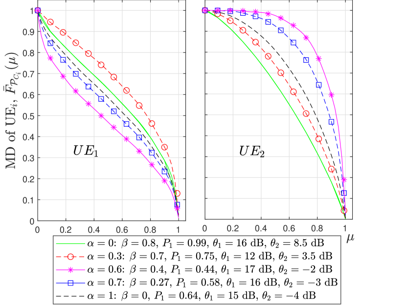
Figure 3: MD vs. $\mu$ using optimum RA for each $\alpha$ with TMT $=0.25$.

Fig. 3 is a plot of the MD, using both the exact moments (Lemma 1) and the approximate moments (Lemma 4), for $\alpha=0.3$ and $\alpha=1$, traditional NOMA, using fixed RA. The figure validates the analysis in Section III as the simulation results are a tight match with the exact moments. The approximate moments are not as close to the simulation but follow the same trends which still gives insights on network performance at a lower computational cost. As anticipated, due to the opposing natures of A1 and A2, the approximate moments can both underestimate and overestimate the MD. Focusing on the exact moments, we observe that for $\alpha=0.3$, $93\%$ of $\text{\lx@glossaries@gls@link{acronym}{ue}{\leavevmode UE}}_{1}$ and $78.2\%$ of $\text{\lx@glossaries@gls@link{acronym}{ue}{\leavevmode UE}}_{2}$ achieve a reliability of $0.8$. With $\alpha=1$, on the other hand, only $81.9\%$ of $\text{\lx@glossaries@gls@link{acronym}{ue}{\leavevmode UE}}_{1}$ and $47.7\%$ of $\text{\lx@glossaries@gls@link{acronym}{ue}{\leavevmode UE}}_{2}$ achieve a reliability of $0.8$. Thus, a notable improvement in the percentage of UEs able to achieve the same reliability is observed for both UEs (13.5 % increase for $\text{\lx@glossaries@gls@link{acronym}{ue}{\leavevmode UE}}_{1}$ and 63.9 % for $\text{\lx@glossaries@gls@link{acronym}{ue}{\leavevmode UE}}_{2}$) in pNOMA compared to NOMA. We also observe that the 5%-user performance that network operators are often interested in, defined as the reliability that 95% of the UEs achieve but 5% do not, has similar trends. With $\alpha=0.3$, 95% of $\text{\lx@glossaries@gls@link{acronym}{ue}{\leavevmode UE}}_{1}$ ($\text{\lx@glossaries@gls@link{acronym}{ue}{\leavevmode UE}}_{2}$) achieve a reliability of 0.76 (0.58), while in NOMA, they achieve a reliability of 0.55 (0.245). These results emphasize the significance of the partial overlap on percentile performance.

Fig. 3 plots the MD for different $\alpha$ values using fixed RA. We observe that in general, when RA is fixed, increasing $\alpha$ deteriorates the performance of $\text{\lx@glossaries@gls@link{acronym}{ue}{\leavevmode UE}}_{2}$ due to the increasing $\mathcal{I}(\alpha,\beta)$ and consequently, interference. Thus the percentage of $\text{\lx@glossaries@gls@link{acronym}{ue}{\leavevmode UE}}_{2}$ that can achieve at least a certain coverage probability $\mu$ decreases with $\alpha$. The performance of $\text{\lx@glossaries@gls@link{acronym}{ue}{\leavevmode UE}}_{1}$, on the other hand, is more complex as it first deteriorates as $\alpha$ increases from $0$ to $0.5$ and then improves from $\alpha=0.5$ to $1$. When $\alpha\leq 0.5$, $\text{\lx@glossaries@gls@link{acronym}{ue}{\leavevmode UE}}_{1}$ treats the message of $\text{\lx@glossaries@gls@link{acronym}{ue}{\leavevmode UE}}_{2}$ as noise; increasing $\alpha$ increases $\mathcal{I}(\alpha,\beta)$ and therefore the IaCI from $\text{\lx@glossaries@gls@link{acronym}{ue}{\leavevmode UE}}_{2}$, thereby deteriorating the performance of $\text{\lx@glossaries@gls@link{acronym}{ue}{\leavevmode UE}}_{1}$. When $\alpha>0.5$, there is a switch in decoding technique and the message of $\text{\lx@glossaries@gls@link{acronym}{ue}{\leavevmode UE}}_{2}$ is decoded by $\text{\lx@glossaries@gls@link{acronym}{ue}{\leavevmode UE}}_{1}$ before decoding its own message; increasing $\alpha$ and therefore $\mathcal{I}(\alpha,\beta)$ in this case increases the power of $\text{\lx@glossaries@gls@link{acronym}{ue}{\leavevmode UE}}_{2}$’s message making it easier to decode, thereby improving the performance of $\text{\lx@glossaries@gls@link{acronym}{ue}{\leavevmode UE}}_{1}$. Thus, in Fig. 3, for $\text{\lx@glossaries@gls@link{acronym}{ue}{\leavevmode UE}}_{1}$ pNOMA outperforms NOMA ($\alpha=1$) only when $\alpha\leq 0.4$, while for $\text{\lx@glossaries@gls@link{acronym}{ue}{\leavevmode UE}}_{2}$ pNOMA always outperforms NOMA.

Fig. 3 plots the MD for different $\alpha$ values using the optimum RA associated with $\text{\lx@glossaries@gls@link{acronym}{tmt}{\leavevmode TMT}}=0.25$. Unlike Fig. 3, the RA here is not the same for all $\alpha$ values and is specified in the legend for each $\alpha$. The performance of $\text{\lx@glossaries@gls@link{acronym}{ue}{\leavevmode UE}}_{2}$ increases with $\alpha$ from $0$ to $0.6$. This occurs because increasing $\alpha$ increases $\text{BW}_{2}$, lowering the $\theta_{2}$ required to achieve $\text{\lx@glossaries@gls@link{acronym}{tmt}{\leavevmode TMT}}=0.25$. Increasing $\alpha$ beyond $0.6$ decreases the performance of $\text{\lx@glossaries@gls@link{acronym}{ue}{\leavevmode UE}}_{2}$ as the dominance of the growing impact of $\mathcal{I}(\alpha,\beta)$ increases interference. While $\text{\lx@glossaries@gls@link{acronym}{ue}{\leavevmode UE}}_{2}$ aims to use the minimum resources to achieve TMT, the goal of $\text{\lx@glossaries@gls@link{acronym}{ue}{\leavevmode UE}}_{1}$ is to achieve the largest possible throughput. The performance in terms of the MD for $\text{\lx@glossaries@gls@link{acronym}{ue}{\leavevmode UE}}_{1}$ initially increases from $\alpha=0$ to $0.3$, as the increasing $\text{BW}_{1}$ reduces the $\theta_{1}$ required to achieve maximum throughput. The performance decreases as $\alpha$ is increased to 0.6. This is attributed to the switch in decoding decoding at higher $\alpha$. As $\mathcal{I}(\alpha,\beta)$ is not very high in this regime, decoding $\text{\lx@glossaries@gls@link{acronym}{ue}{\leavevmode UE}}_{2}$’s message is difficult for $\text{\lx@glossaries@gls@link{acronym}{ue}{\leavevmode UE}}_{1}$, and thus $\text{\lx@glossaries@gls@link{acronym}{ue}{\leavevmode UE}}_{1}$’s performance suffers. Increasing $\alpha$ beyond 0.6 improves performance as the higher $\mathcal{I}(\alpha,\beta)$ makes decoding $\text{\lx@glossaries@gls@link{acronym}{ue}{\leavevmode UE}}_{2}$’s message easier for $\text{\lx@glossaries@gls@link{acronym}{ue}{\leavevmode UE}}_{1}$ and as the increasing BW for both UEs allows more power to be left for $\text{\lx@glossaries@gls@link{acronym}{ue}{\leavevmode UE}}_{1}$’s message.

We observe, from Figs. 3 and 3 explicitly, that $\text{\lx@glossaries@gls@link{acronym}{ue}{\leavevmode UE}}_{2}$ with the appropriate $\alpha$ outperforms its NOMA counterpart more than $\text{\lx@glossaries@gls@link{acronym}{ue}{\leavevmode UE}}_{1}$. This can be attributed to the additional flexibility that comes with the ability to select $\alpha$ and $\beta$ in pNOMA, which are fixed in NOMA. The observation sheds light on the fact that with appropriate $\alpha$, pNOMA is able to assist the weaker UE significantly more than NOMA highlighting the role of pNOMA in improving UE fairness.

V Conclusion

The MD of a pNOMA network was studied to obtain fine-grained information on network performance. Integral expressions were obtained for the moments of the CCP. We reduced the integrals for the first two moments, which are required for approximating the MD via moment matching. By proposing the use of two approximations, accurate approximate moments of the CCP were derived that further simplified the integral calculation. We showed that in terms of percentile performance of links, pNOMA outperforms NOMA only when $\alpha$ is lower than a certain value. This highlights that deploying pNOMA over NOMA is only efficient when $\alpha$ is low and sheds light on careful parameter selection. Our results also indicated that pNOMA helps improve the performance of weaker UEs highlighting its significance as a means to improve UE fairness.

References

[1]
K. S. Ali, E. Hossain, and M. J. Hossain, “Partial non-orthogonal
multiple access (NOMA) in downlink Poisson networks,” IEEE Trans.
Wireless Commun., vol. 19, no. 11, pp. 7637–7652, 2020.
[2]
B. Blaszczyszyn et al., Stochastic Geometry Analysis of Cellular
Networks. Cambridge University Press,
2018.
[3]
H. ElSawy et al., “Modeling and analysis of cellular networks using
stochastic geometry: A tutorial,” IEEE Commun. Surveys and Tutorials,
vol. 19, no. 1, pp. 167–203, Firstquarter 2017.
[4]
K. S. Ali, M. Haenggi, H. E. Sawy, A. Chaaban, and M. Alouini, “Downlink
non-orthogonal multiple access (NOMA) in Poisson networks,” IEEE
Trans. Commun., vol. 67, no. 2, pp. 1613–1628, Feb. 2019.
[5]
K. S. Ali, H. Elsawy, A. Chaaban, and M. S. Alouini, “Non-orthogonal multiple
access for large-scale 5G networks: Interference aware design,” IEEE
Access, vol. 5, pp. 21 204–21 216, 2017.
[6]
H. Tabassum, E. Hossain, and M. J. Hossain, “Modeling and analysis of uplink
non-orthogonal multiple access (NOMA) in large-scale cellular networks
using poisson cluster processes,” IEEE Trans. Commun., vol. 65,
no. 8, pp. 3555–3570, Aug. 2017.
[7]
Z. Zhang, H. Sun, and R. Q. Hu, “Downlink and uplink non-orthogonal multiple
access in a dense wireless network,” IEEE J. Selec. Areas Commun.,
vol. 35, no. 12, pp. 2771–2784, Dec. 2017.
[8]
Z. Zhang, H. Sun, R. Q. Hu, and Y. Qian, “Stochastic geometry based
performance study on 5G non-orthogonal multiple access scheme,” in
Proc. of IEEE Global Commun. Conf., Dec. 2016, pp. 1–6.
[9]
K. S. Ali, H. E. Sawy, and M. Alouini, “Meta distribution of downlink
non-orthogonal multiple access (NOMA) in Poisson networks,” IEEE
Wireless Comm. Letters, vol. 8, no. 2, pp. 572–575, Apr. 2019.
[10]
M. Salehi, H. Tabassum, and E. Hossain, “Meta distribution of SIR in
large-scale uplink and downlink NOMA networks,” IEEE Transactions on
Communications, vol. 67, no. 4, pp. 3009–3025, 2019.
[11]
P. D. Mankar and H. S. Dhillon, “Meta distribution for downlink NOMA in
cellular networks with 3GPP-inspired user ranking,” in 2019 IEEE
Global Communications Conf. (GLOBECOM), 2019, pp. 1–6.
[12]
M. Haenggi, “The meta distribution of the SIR in Poisson bipolar and
cellular networks,” IEEE Trans. Wireless Commun., vol. 15, no. 4, pp.
2577–2589, Apr. 2016.
[13]
A. AlAmmouri et al., “In-band -duplex scheme for cellular
networks: A stochastic geometry approach,” IEEE Trans. Wireless
Commun., vol. 15, no. 10, pp. 6797–6812, Oct. 2016.
[14]
H. A. David, Order statistics. NJ: John Wiley, 1970.
[15]
R. K. Ganti and M. Haenggi, “Asymptotics and approximation of the SIR
distribution in general cellular networks,” IEEE Trans. Wireless
Commun., vol. 15, no. 3, pp. 2130–2143, Mar. 2016.