Optimization Guarantees of Unfolded ISTA and ADMM Networks With Smooth Soft-Thresholding

Abstract

Solving linear inverse problems plays a crucial role in numerous applications. Algorithm unfolding based, model-aware data-driven approaches have gained significant attention for effectively addressing these problems. Learned iterative soft-thresholding algorithm (LISTA) and alternating direction method of multipliers compressive sensing network (ADMM-CSNet) are two widely used such approaches, based on ISTA and ADMM algorithms, respectively. In this work, we study optimization guarantees, i.e., achieving near-zero training loss with the increase in the number of learning epochs, for finite-layer unfolded networks such as LISTA and ADMM-CSNet with smooth soft-thresholding in an over-parameterized (OP) regime. We achieve this by leveraging a modified version of the Polyak-Łojasiewicz, denoted PL^∗, condition. Satisfying the PL^∗ condition within a specific region of the loss landscape ensures the existence of a global minimum and exponential convergence from initialization using gradient descent based methods. Hence, we provide conditions, in terms of the network width and the number of training samples, on these unfolded networks for the PL^∗ condition to hold. We achieve this by deriving the Hessian spectral norm of these networks. Additionally, we show that the threshold on the number of training samples increases with the increase in the network width. Furthermore, we compare the threshold on training samples of unfolded networks with that of a standard fully-connected feed-forward network (FFNN) with smooth soft-thresholding non-linearity. We prove that unfolded networks have a higher threshold value than FFNN. Consequently, one can expect a better expected error for unfolded networks than FFNN.

I Introduction

Linear inverse problems are fundamental in many engineering and science applications [1, 2], where the aim is to recover a vector of interest or target vector from an observation vector. Existing approaches to address these problems can be categorized into two types; model-based and data-driven. Model-based approaches use mathematical formulations that represent knowledge of the underlying model, which connects observation and target information. These approaches are simple, computationally efficient, and require accurate model knowledge for good performance [3, 4]. In data-driven approaches, a machine learning (ML) model, e.g., a neural network, with a training dataset, i.e., a supervised setting, is generally considered. Initially, the model is trained by minimizing a certain loss function. Then, the trained model is used on unseen test data. Unlike model-based methods, data-driven approaches do not require underlying model knowledge. However, they require a large amount of data and huge computational resources while training [3, 4].

By utilizing both domains’ knowledge, i.e., the mathematical formulation of the model and ML ability, a new approach, called model-aware data-driven, has been introduced [5, 6]. This approach involves the construction of a neural network architecture based on an iterative algorithm, which solves the optimization problem associated with the given model. This process is called algorithm unrolling or unfolding [6]. It has been observed that the performance, in terms of accurate recovery of the target vector, training data requirements, and computational complexity, of model-aware data-driven networks is better when compared with existing techniques [5, 7]. Learned iterative soft-thresholding algorithm (LISTA) and alternating direction method of multipliers compressive sensing network (ADMM-CSNet) are two popular unfolded networks that have been used in many applications such as image compressive sensing [7], image deblurring [8], image super-resolution [9], super-resolution microscopy [10], clutter suppression in ultrasound [11], power system state estimation [12], and many more.

Nevertheless, the theoretical studies supporting these unfolded networks remain to be established. There exist a few theoretical studies that address the challenges of generalization [13, 14, 15] and convergence rate [16, 17, 18] in unfolded networks. For instance, in [13], the authors showed that unfolded networks exhibit higher generalization capability compared with standard ReLU networks by deriving an upper bound on the generalization and estimation errors. In [16, 17, 18] the authors examined the LISTA network convergence to the ground truth as the number of layers increases i.e., layer-wise convergence (which is analogous to iteration-wise convergence in the ISTA algorithm). Furthermore, in [16, 17, 18], the network weights are not learned but are calculated in an analytical way (by solving a data-free optimization problem). Thus, the network only learns a few parameters, like threshold, step size, etc., from the available data. In this work, we study guarantees to achieve near-zero training loss with an increase in the number of learning epochs, i.e., optimization guarantees, by using gradient descent (GD) for both LISTA and ADMM-CSNet with smooth activation in an over-parameterized regime. Note that, our work differs from [16, 17, 18], as we focus on the convergence of training loss with the increase in the number of epochs by fixing the number of layers in the network.

In classical ML theory, we aim to minimize the expected/test risk by finding a balance between under-fitting and over-fitting, i.e., achieving the bottom of the classical U-shaped test risk curve [19]. However, modern ML results establish that large models that try to fit train data exactly, i.e., interpolate, often show high test accuracy even in the presence of noise [20, 21, 22, 23, 24, 25]. Recently, ML practitioners proposed a way to numerically justify the relationship between classical and modern ML practices. They achieved this by proposing a performance curve called the double-descent test risk curve [20, 21, 23, 24], which is depicted in Fig. 1.

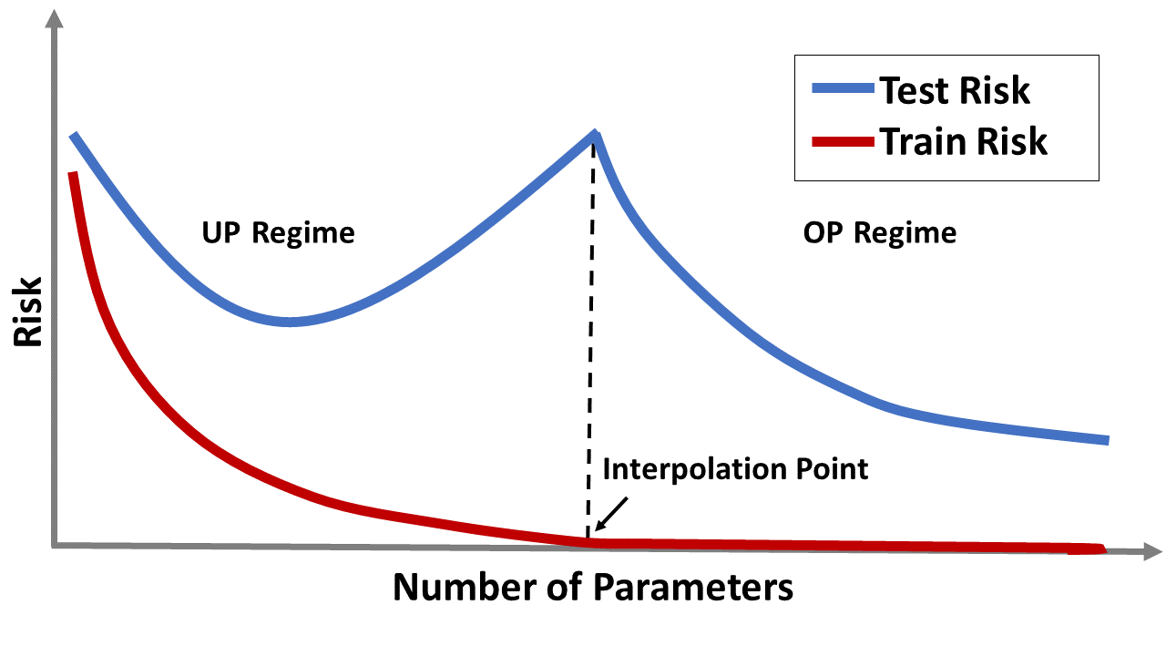
Figure 1: Double descent risk curve.

This curve shows that increasing the model capacity (e.g., model parameters) until interpolation results in the classical U-shaped risk curve; further increasing it beyond the interpolation point reduces the test risk. Thus, understanding the conditions – as a function of the training data – that allow perfect data fitting is crucial.

Neural networks can be generally categorized into under-parameterized (UP) and over-parameterized (OP), based on the number of trainable parameters and the number of training data samples. If the number of trainable parameters is less than the number of training samples, then the network is referred to as an UP model, else, referred to as an OP model. The loss landscape of both UP and OP models is generally non-convex. However, OP networks satisfy essential non-convexity [26]. Particularly, the loss landscape of an OP model has a non-isolated manifold of global minima with non-convexity around any small neighborhood of a global minimum. Despite being highly non-convex, GD based methods work well for training OP networks [27, 28, 29, 30]. Recently, in [26, 31], the authors provided a theoretical justification for this. Specifically, they proved that the loss landscape, corresponding to the squared loss function, of a typical smooth OP model holds the modified version of the Polyak-Łojasiewicz condition, denoted PL^∗, on most of the parameter space. Indeed, a necessary (but not sufficient) condition to satisfy the PL^∗ is that the model should be in OP regime. Satisfying PL^∗ on a region in the parameter space guarantees the existence of a global minimum in that region, and exponential convergence to the global minimum from the Gaussian initialization using simple GD.

Motivated by the aforementioned PL^∗-based mathematical framework of OP networks, in this paper, we analyze optimization guarantees of finite-layer OP based unfolded ISTA and ADMM networks. Moreover, as the analysis of PL^∗ depends on the double derivative of the model [26], we consider a smooth version of the soft-thresholding as an activation function. The major contributions of the paper are summarized as follows:

• As the linear inverse problem aims to recover a vector, we initially extend the gradient-based optimization analysis of the OP model with a scalar output, proposed in [26], to a vector output. In the process, we prove that a necessary condition to satisfy PL^∗ is $P\gg mT$, where $P$ denotes the number of parameters, $m$ is the dimension of the model output vector, and $T$ denotes the number of training samples.

• In [31, 26], the authors provided a condition on the width of a fully-connected feed-forward neural network (FFNN) with scalar output to satisfy the PL^∗ condition by utilizing the Hessian spectral norm of the network. Motivated by this work, we derive the Hessian spectral norm of finite-layer LISTA and ADMM-CSNet with smoothed soft-thresholding non-linearity. We show that the norm is on the order of $\tilde{\Omega}\left(1/\sqrt{m}\right)$, where $m$ denotes the width of the network which is equal to the target vector dimension.

• By employing the Hessian spectral norm, we derive necessary conditions on both $m$ and $T$ to satisfy the PL^∗ condition for both LISTA and ADMM-CSNet. Moreover, we demonstrate that the threshold on $T$, which denotes the maximum number of training samples that a network can memorize, increases as the network width increases.

• We compare the threshold on the number of training samples of LISTA and ADMM-CSNet with that of FFNN, solving a given linear inverse problem. Our findings show that LISTA/ADMM-CSNet exhibits a higher threshold value than FFNN. Specifically, we demonstrate this by proving that the upper bound on the minimum eigenvalue of the tangent kernel matrix at initialization is high for LISTA/ADMM-CSNet compared to FFNN. This implies that, with fixed network parameters, the unfolded network is capable of memorizing a larger number of training samples compared to FFNN. Therefore, we should expect to obtain a better expected error (which is upper bounded by the sum of generalization and training error [32]) for unfolded networks than FFNN.

• Additionally, we numerically evaluate the parameter efficiency of unfolded networks in comparison to FFNNs. In particular, we demonstrate that FFNNs require a higher number of parameters to achieve near-zero empirical training loss compared to LISTA/ADMM-CSNet for a given fixed $T$ value.

Outline: The paper is organized as follows: Section II presents a comprehensive discussion on LISTA and ADMM-CSNet, and also formulates the problem. Section III extends the PL^∗-based optimization guarantees of an OP model with scalar output to a model with multiple outputs. Section IV begins by deriving the Hessian spectral norm of the unfolded networks. Then, it provides conditions on the network width and on the number of training samples to satisfy the PL^∗ condition. Further, it also establishes a comparative analysis of the threshold for the number of training samples among LISTA, ADMM-CSNet, and FFNN. Section V discusses the experimental results and Section VI draws conclusions.

Notations: The following notations are used throughout the paper. The set of real numbers is denoted by $\mathbb{R}$. We use bold lowercase letters, e.g., $\mathbf{y}$, for vectors, capital letters, e.g., ${W}$, for matrices, and bold capital letters, e.g., $\mathbf{H}$, for tensors. Symbols $||\mathbf{z}||_{1}$, $||\mathbf{z}||$, and $||\mathbf{z}||_{\infty}$ denote the $l_{1}$-norm, $l_{2}$-norm, and $l_{\infty}$-norm of $\mathbf{z}$, respectively. The spectral norm and Frobenius norm of a matrix ${W}$ are written as $||W||$ and $||W||_{F}$, respectively. We use $[L]$ to denote the set $\{1,2,\dots,L\}$, where $L$ is a natural number. The first-order derivative or gradient of a function $L(\mathbf{w})$ w.r.t. $\mathbf{w}$ is denoted as $\nabla_{\mathbf{w}}L(\mathbf{w})$. The asymptotic upper bound and lower bound on a quantity are described using $O(\cdot)$ and $\Omega(\cdot)$, respectively. Notations $\tilde{O}(\cdot)$ and $\tilde{\Omega}(\cdot)$ are used to suppress the logarithmic terms in $O(\cdot)$ and $\Omega(\cdot)$, respectively. For example, $O\left(\frac{1}{m}\ln(m)\right)$ is written as $\tilde{O}\left(\frac{1}{m}\right)$. Symbols $\gg$ and $\ll$ mean “much greater than” and “much lesser than”, respectively. Consider a matrix $G$ with $G_{i,j}=\sum_{k}A_{i,j,k}v_{k}$, where $A_{i,j,k}$ is a component in tensor $\mathbf{A}\in\mathbb{R}^{m_{1}\times m_{2}\times m_{3}}$. The spectral norm of $G$ can be bounded as

$$\|G\|\leq\|\mathbf{A}\|_{2,2,1}\|\mathbf{v}\|_{\infty}.$$ (1)

Here $\|\mathbf{A}\|_{2,2,1}$ denotes the $(2,2,1)$-norm of the tensor $\mathbf{A}$, which is defined as

$$\|\mathbf{A}\|_{2,2,1}={\sup\limits_{\|\mathbf{r}\|=\|\mathbf{s}\|=1}}\sum\limits_{k=1}^{m_{3}}\left|\sum\limits_{i=1}^{m_{1}}\sum\limits_{j=1}^{m_{2}}A_{i,j,k}r_{i}s_{j}\right|,$$ (2)

where $\mathbf{r}\in\mathbb{R}^{m_{1}\times 1}$ and $\mathbf{s}\in\mathbb{R}^{m_{2}\times 1}$.

II Problem Formulation

II-A LISTA and ADMM-CSNet

Consider the following linear inverse problem

$$\mathbf{y}={A}\mathbf{x}+\mathbf{e}.$$ (3)

Here $\mathbf{y}\in\mathbb{R}^{n\times 1}$ is the observation vector, $\mathbf{x}\in\mathbb{R}^{m\times 1}$ is the target vector, ${A}\in\mathbb{R}^{n\times m}$ is the forward linear operator matrix with $m>n$, and $\mathbf{e}$ is noise with $\|\mathbf{e}\|_{2}<\epsilon$, where the constant $\epsilon>0$. Our aim is to recover $\mathbf{x}$ from a given $\mathbf{y}$.

In model-based approaches, an optimization problem is formulated using some prior knowledge about the target vector and is usually solved using an iterative algorithm. For instance, by assuming $\mathbf{x}$ is a $k$-sparse vector [33], the least absolute shrinkage and selection operator (LASSO) problem is formulated as

$${\operatorname*{\,min}_{\mathbf{x}}}\ \frac{1}{2}\|\mathbf{y}-A\mathbf{x}\|^{2}+\gamma\|\mathbf{x}\|_{1},$$ (4)

where $\gamma$ is a regularization parameter. Iterative algorithms, such as ISTA and ADMM [34], are generally used to solve the LASSO problem. The update of $\mathbf{x}$ at the $l^{\text{th}}$ iteration in ISTA is [35]

$$\mathbf{x}^{l}=S_{\gamma\tau}\left\{\left(\mathbf{I}-\tau{A}^{T}{A}\right)\mathbf{x}^{l-1}+{\tau}{A}^{T}\mathbf{y}\right\},$$ (5)

where $\mathbf{x}^{0}$ is a bounded input initialization, $\tau$ controls the iteration step size, and $S_{\lambda}(\cdot)$ is the soft-thresholding operator applied element-wise on a vector argument $S_{\lambda}(x)=\text{sign}(x)\text{max}\left(|x|-\lambda,0\right).$ The $l^{\text{th}}$ iteration in ADMM is [36]

$$\mathbf{x}^{l} =\left(A^{T}A+\rho\mathbf{I}\right)^{-1}\left({A}^{T}\mathbf{y}+\rho\left(\mathbf{z}^{l-1}-\mathbf{u}^{l-1}\right)\right),$$ (6)

$$\mathbf{z}^{l} =S_{\frac{\gamma}{\rho}}\left(\mathbf{x}^{l}+\mathbf{u}^{l-1}\right),$$

$$\mathbf{u}^{l} =\mathbf{u}^{l-1}+\left(\mathbf{x}^{l}-\mathbf{z}^{l}\right),$$

where $\mathbf{x}^{0}$, $\mathbf{z}^{0}$, and $\mathbf{u}^{0}$, are bounded input initializations to the network and $\rho>0$ is a penalty parameter. Model-based approaches are in general sensitive to inaccurate knowledge of the underlying model [3, 4]. In turn, data-driven approaches use an ML model to recover the target vector. These approaches generally require a large amount of training data and computational resources [3, 4].

A model-aware data-driven approach is generally developed using algorithm unfolding or unrolling [6]. In unfolding, a neural network is constructed by mapping each iteration in the iterative algorithm (such as (5) or (6)) to a network layer. Hence, an iterative algorithm with $L$-iterations leads to an $L$-layer cascaded deep neural network. The network is then trained by using the available dataset containing a series of pairs $\{\mathbf{y}_{i},\mathbf{x}_{i}\},i\in[T]$. For example, the update of $\mathbf{x}$ at the $l^{\text{th}}$ iteration in ISTA, given in (5), is rewritten as

$$\mathbf{x}^{l}=S_{\lambda}\left\{{W}_{2}^{l}\mathbf{x}^{l-1}+W_{1}^{l}\mathbf{y}\right\},$$ (7)

where $\lambda=\gamma\tau$, $W_{1}^{l}=\tau{A}^{T}$, and $W_{2}^{l}=\mathbf{I}-\tau{A}^{T}{A}$. By considering $W_{1}^{l}$, $W_{2}^{l}$, and $\lambda$ as network learnable parameters, one can map the above $l^{\text{th}}$ iteration to an $l^{\text{th}}$ layer in the network as shown in Fig. 2. The corresponding unfolded network is called learned ISTA (LISTA) [5].

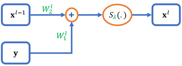
Figure 2: $l^{\text{th}}$ layer of the unfolded ISTA network.

Similarly, by considering $W_{1}^{l}=\left(A^{T}A+\rho\mathbf{I}\right)^{-1}{A}^{T}$, $W_{2}^{l}=\left(A^{T}A+\rho\mathbf{I}\right)^{-1}\rho$, and $\lambda=\frac{\gamma}{\rho}$ as learnable parameters, (6) is rewritten as

$$\mathbf{x}^{l} =W_{1}^{l}\mathbf{y}+W_{2}^{l}\left(\mathbf{z}^{l-1}-\mathbf{u}^{l-1}\right),$$ (8)

$$\mathbf{z}^{l} =S_{\lambda}\left(\mathbf{x}^{l}+\mathbf{u}^{l-1}\right),$$

$$\mathbf{u}^{l} =\mathbf{u}^{l-1}+\left(\mathbf{x}^{l}-\mathbf{z}^{l}\right).$$

The above $l^{\text{th}}$ iteration in ADMM can be mapped to an $l^{\text{th}}$ layer in a network as shown in Fig. 3, leading to ADMM-CSNet [7]. Note that from a network point of view, the inputs of $l^{\text{th}}$ layer are $\mathbf{x}^{l-1}$ and $\mathbf{y}$ for LISTA, and $\mathbf{z}^{l-1}$, $\mathbf{u}^{l-1}$ and $\mathbf{y}$ for ADMM-CSNet.

Figure 3: $l^{\text{th}}$ layer of the unfolded ADMM network.

It has been observed that the performance of LISTA and ADMM-CSNet is better in comparison with ISTA, ADMM, and traditional networks, in many applications [5, 7]. For instance, to achieve good performance the number of layers required in an unrolled network is generally much smaller than the number of iterations required by the iterative solver [5]. In addition, an unrolled network works effectively even if the linear operator matrix, ${A}$, is not known exactly. An unrolled network typically requires less data for training compared to standard deep neural networks [3] to achieve a certain level of performance on unseen data. Due to these advantages, LISTA and ADMM-CSNet have been used in many applications [7, 8, 9, 10, 11, 12]. That said, the theoretical foundations supporting these networks remain to be established. While there have been some studies focusing on the generalization [13, 14, 15] and convergence rate [16, 17, 18] of unfolded networks, a comprehensive study of the optimization guarantees is lacking. Here, we analyze the conditions on finite $L$-layer LISTA and ADMM-CSNet to achieve near-zero training loss with the increase in the number of epochs.

II-B Problem Formulation

We consider the following questions: Under what conditions does the training loss in LISTA and ADMM-CSNet converge to zero as the number of epochs tends to infinity using GD? Additionally, how do these conditions differ for FFNNs?

For the analysis, we consider the following training setting: Let $\mathbf{x}=F(\mathbf{w},\lambda;\mathbf{y})$ be an $L$-layer unfolded model, where $\mathbf{y}\in\mathbb{R}^{n\times 1}$ is the model input vector, $\mathbf{x}\in\mathbb{R}^{m\times 1}$ is the model output, and $\mathbf{w}\in\mathbb{R}^{P\times 1}$ and $\lambda$ are the learnable parameters. To simplify the analysis, $\lambda$ is assumed to be constant, henceforth, we write $F(\mathbf{w},\lambda;\mathbf{y})$ as $F(\mathbf{w};\mathbf{y})$. This implies that $\mathbf{w}_{P\times 1}=\text{Vec}\left([\mathbf{W}]_{L\times m\times(m+n)}\right)$ is the only learnable (untied) parameter vector, where

$$\mathbf{W}=\left[W^{1}\ W^{2}\ \dots\ W^{L}\right],$$ (9)

and $\left[W^{l}\right]_{m\times(m+n)}=\left[W_{1}^{l}\ \ W_{2}^{l}\right]$ is the parameter matrix corresponding to the $l^{\text{th}}$-layer. Alternatively, we can write

$$\mathbf{W}=\left[\left[\mathbf{W}_{1}\right]_{L\times m\times n}\ \ \left[\mathbf{W}_{2}\right]_{L\times m\times m}\right],$$ (10)

$\mathbf{W}_{1}=\left[W_{1}^{1}\ \dots\ W_{1}^{L}\right]$ and $\mathbf{W}_{2}=\left[W_{2}^{1}\ \dots\ W_{2}^{L}\right]$. Consider the training dataset $\left\{\mathbf{y}_{i},\mathbf{x}_{i}\right\}_{i=1}^{T}$. An optimal parameter vector $\mathbf{w}^{*}$, such that $F(\mathbf{w}^{*};\mathbf{y}_{i})\approx\mathbf{x}_{i},\ \forall i\in[T]$, is found by minimizing an empirical loss function $L(\mathbf{w})$, defined as

$$L(\mathbf{w})=\sum_{i=1}^{T}l(\mathbf{f}_{i},\mathbf{x}_{i}),$$ (11)

where $l(\cdot)$ is the loss function, $\mathbf{f}_{i}=(\mathcal{F}(\mathbf{w}))_{i}=F(\mathbf{w},\mathbf{y}_{i})$, $\mathcal{F}(\cdot):\mathbb{R}^{P\times 1}\xrightarrow{}\mathbb{R}^{m\times T}$, and $(\mathcal{F}(\mathbf{w}))_{i}$ is the $i^{\text{th}}$ column in $\mathcal{F}(\mathbf{w})$. We consider the squared loss, hence

$$L(\mathbf{w})=\frac{1}{2}\sum_{i=1}^{T}\|\mathbf{f}_{i}-\mathbf{x}_{i}\|^{2}=\frac{1}{2}\|\mathcal{F}(\mathbf{w})-X\|_{F}^{2},$$ (12)

where ${X}=\left[\mathbf{x}_{1},\dots,\mathbf{x}_{T}\right]$. We choose GD as the optimization algorithm for minimizing $L(\mathbf{w})$, hence, the updating rule is

$$\mathbf{w}_{t+1}=\mathbf{w}_{t}-\eta\nabla_{\mathbf{w}}L(\mathbf{w})$$

where $\eta$ is the learning rate.

Our aim is to derive conditions on LISTA and ADMM-CSNet such that $L(\mathbf{w})$ converges to zero with an increase in the number of epochs using GD, i.e., $\lim_{t\rightarrow\infty}L(\mathbf{w}_{t})=0.$ In addition, we compare these conditions with those of FFNN, where we obtain the conditions for FFNN by extending the analysis given in [26]. Specifically, in Section IV-C, we derive a bound on the number of training samples to achieve near zero training loss for unfolded networks. Further, we show that this threshold is lower for FFNN compared to unfolded networks.

III Revisiting PL^∗-Based Optimization Guarantees

In [26] the authors proposed PL^∗-based optimization theory for a model with a scalar output. Motivated by this, in this section, we extend this theory to a multi-output model, as we aim to recover a vector in a linear inverse problem.

Consider an ML model, not necessarily an unfolded network, $\mathbf{x}=F(\mathbf{w};\mathbf{y})$, with the training setup mentioned in Section II-B, where $\mathbf{y}\in\mathbb{R}^{n\times 1}$, $\mathbf{x}\in\mathbb{R}^{m\times 1}$, and $\mathbf{w}\in\mathbb{R}^{P\times 1}$. Further, assume that the model is $L_{\mathcal{F}}$-Lipschitz continuous and $\beta_{\mathcal{F}}$-smooth. A function $\mathcal{F}(\cdot):\mathbb{R}^{P}\xrightarrow{}\mathbb{R}^{m\times T}$ is $L_{\mathcal{F}}$-Lipschitz continuous if

$$\|\mathcal{F}(\mathbf{w}_{1})-\mathcal{F}(\mathbf{w}_{2})\|_{F}\leq L_{\mathcal{F}}\|\mathbf{w}_{1}-\mathbf{w}_{2}\|,\ \forall\mathbf{w}_{1},\mathbf{w}_{2}\in\mathbb{R}^{P},$$

and is $\beta_{\mathcal{F}}$-smooth if the gradient of the function is $\beta_{\mathcal{F}}$-Lipschitz, i.e.,

$$\|\nabla_{\mathbf{w}}\mathcal{F}(\mathbf{w_{1}})-\nabla_{\mathbf{w}}\mathcal{F}(\mathbf{w_{2}})\|_{F}\leq\beta_{\mathcal{F}}\|\mathbf{w_{1}}-\mathbf{w_{2}}\|,$$

$\forall\mathbf{w}_{1},\ \mathbf{w}_{2}\in\mathbb{R}^{P}$. The Hessian spectral norm of $\mathcal{F}(\cdot)$ is defined as

$$\|\mathbf{H}_{\mathcal{F}}(\mathbf{w})\|=\underset{i\in[T]}{\text{max}}\|\mathbf{H}_{\mathcal{F}_{i}}(\mathbf{w})\|,$$

where $\mathbf{H}_{\mathcal{F}}\in\mathbb{R}^{T\times m\times P\times P}$ is a tensor with $(\mathbf{H}_{\mathcal{F}})_{i,j,k,l}=\frac{\partial^{2}\left(\mathcal{F}(\mathbf{w})\right)_{j,i}}{\partial w_{k}\partial w_{l}}$ and $\mathbf{H}_{\mathcal{F}_{i}}=\frac{\partial^{2}(\mathcal{F}(\mathbf{w}))_{i}}{\partial\mathbf{w}^{2}}$. As stated earlier, the loss landscape of the OP model typically satisfies PL^∗ on most of the parameter space. Formally, the PL^∗ condition is defined as follows [37, 38]:

Definition 1.

Consider a set $C\subset\mathbb{R}^{P\times 1}$ and $\mu>0$. Then, a non-negative function $L(\mathbf{w})$ satisfies $\mu$-PL^∗ condition on $C$ if $\|\nabla_{\mathbf{w}}L(\mathbf{w})\|^{2}\geq\mu L(\mathbf{w}),\ \forall\mathbf{w}\in C$.

Definition 2.

The tangent kernel matrix, $[K(\mathbf{w})]_{mT\times mT}$, of the function $\mathcal{F}(\mathbf{w})$, is a block matrix with $(i,j)^{\text{th}}$ block defined as

$$(K(\mathbf{w}))_{i,j}=\left[\nabla_{\mathbf{w}}\mathbf{f}_{i}\right]_{m\times P}\left[\nabla_{\mathbf{w}}\mathbf{f}_{j}\right]_{P\times m}^{T},\ i\in[T]\text{ and }j\in[T].$$

From the above definitions, we have the following lemma, which is called $\mu$-uniform conditioning [26] of a multi-output model $\mathcal{F}(\mathbf{w})$:

Lemma 1.

$\mathcal{F}(\mathbf{w})$ satisfies $\mu$-PL^∗ on set $C$ if the minimum eigenvalue of the tangent kernel matrix, $K(\mathbf{w})$, is greater than or equal to $\mu$, i.e., $\lambda_{\text{min}}(K(\mathbf{w}))\geq\mu,\ \forall\mathbf{w}\in C$.

Proof.

From (12), we have $\begin{aligned} \|\nabla_{\mathbf{w}}L(\mathbf{w})\|^{2}&=\left[\hat{\mathbf{f}}-\hat{\mathbf{x}}\right]^{T}\left[\nabla_{\mathbf{w}}\hat{\mathbf{f}}\right]_{mT\times P}\left[\nabla_{\mathbf{w}}\hat{\mathbf{f}}\right]^{T}_{P\times mT}\left[\hat{\mathbf{f}}-\hat{\mathbf{x}}\right]\\ &=\left[\hat{\mathbf{f}}-\hat{\mathbf{x}}\right]^{T}\left[K(\mathbf{w})\right]_{mT\times mT}\left[\hat{\mathbf{f}}-\hat{\mathbf{x}}\right],\end{aligned}$ where $\hat{\mathbf{f}}=\text{Vec}\left(\mathcal{F}(\mathbf{w})\right)$ and $\hat{\mathbf{x}}=\text{Vec}\left(X\right)$. The above equation can be lower-bounded as

$$\|\nabla_{\mathbf{w}}L(\mathbf{w})\|^{2}\geq\lambda_{\text{min}}\left(K(\mathbf{w})\right)\|\hat{\mathbf{f}}-\hat{\mathbf{x}}\|_{2}^{2}\geq\mu L(\mathbf{w}).$$

∎

Observe that $K(\mathbf{w})$ is a positive semi-definite matrix. Thus, a necessary condition to satisfy the PL^∗ condition (that is, a necessary condition to obtain a full rank $K(\mathbf{w})$), for a multi-output model is $P\gg mT$. For a scalar output model, the equivalent condition is $P\gg T$ [26]. Note that if $P\ll T$, i.e., an UP model with a scalar output, then $\lambda_{\text{min}}(K(\mathbf{w}))=0$, implies that an UP model does not satisfy the PL^∗ condition.

Practically, computing $\lambda_{\text{min}}(K(\mathbf{w}))$ for every $\mathbf{w}\in C$, to verify the PL^∗ condition, is not feasible. One can overcome this by using the Hessian spectral norm of the model $\|\mathbf{H}_{\mathcal{F}}(\mathbf{w})\|$ [26]:

Theorem 1.

Let $\mathbf{w}_{0}\in\mathbb{R}^{P\times 1}$ be the parameter initialization of an $L_{\mathcal{F}}$-Lipschitz and $\beta_{\mathcal{F}}$-smooth model $\mathcal{F}(\mathbf{w})$, and $B(\mathbf{w}_{0},R)=\{\mathbf{w}|\ \|\mathbf{w}-\mathbf{w}_{0}\|\leq R\}$ be a ball with radius $R>0$. Assume that $K(\mathbf{w}_{0})$ is well conditioned, i.e., $\lambda_{\text{min}}(K(\mathbf{w}_{0}))=\lambda_{0}$ for some $\lambda_{0}>0$. If $\|\mathbf{H}_{\mathcal{F}}(\mathbf{w})\|\leq\frac{\lambda_{0}-\mu}{2{L_{\mathcal{F}}}\sqrt{T}R}$ for all $\mathbf{w}\in B(\mathbf{w}_{0},R)$, then the model satisfies $\mu$-uniform conditioning in $B(\mathbf{w}_{0},R)$; this also implies that $L(\mathbf{w})$ satisfies $\mu$-PL^∗ in the ball $B(\mathbf{w}_{0},R)$.

The intuition behind the above theorem is that small $\|\mathbf{H}_{\mathcal{F}}(\mathbf{w})\|$ leads to a small change in the tangent kernel. Precisely, if the tangent kernel is well conditioned at the initialization, then a small $\|\mathbf{H}_{\mathcal{F}}(\mathbf{w})\|$ in $B(\mathbf{w}_{0},R)$ guarantees that the tangent kernel is well conditioned within $B(\mathbf{w}_{0},R)$. The following theorem states that satisfying PL^∗ guarantees the existence of a global minimum and exponential convergence to the global minimum from $\mathbf{w}_{0}$ using GD:

Theorem 2.

Consider a model $\mathcal{F}(\mathbf{w})$ that is $L_{\mathcal{F}}$-Lipschitz continuous and $\beta_{\mathcal{F}}$-smooth. If the square loss function $L(\mathbf{w})$ satisfies the $\mu$-PL^∗ condition in $B(\mathbf{w}_{0},R)$ with $R=\frac{2L_{\mathcal{F}}\|\mathcal{F}(\mathbf{w}_{0})-X\|_{F}}{\mu}=O\left(\frac{1}{\mu}\right)$, then we have the following:

• There exist a global minimum, $\mathbf{w}^{*}$, in $B(\mathbf{w}_{0},R)$ such that $\mathcal{F}(\mathbf{w}^{*})=X$.

• GD with step size $\eta\leq\frac{1}{L_{\mathcal{F}}^{2}+\beta_{\mathcal{F}}\|\mathcal{F}(\mathbf{w}_{0})-X\|_{F}}$ converges to a global minimum at an exponential convergence rate, specifically, $L(\mathbf{w}_{t})\leq(1-\eta\mu)^{t}L(\mathbf{w}_{0}).$

The proofs of Theorems 1 and 2 are similar to the proofs of Theorems $2$ and $6$, respectively, in [26]. However, as linear inverse problems deal with vector recovery, the proofs rely on Frobenius norms instead of Euclidean norms.

IV Optimization Guarantees

We now analyze the optimization guarantees of both LISTA and ADMM-CSNet by considering them in the OP regime. Hence, the aim is further simplified to study under what conditions LISTA and ADMM-CSNet satisfy the PL^∗ condition. As mentioned in Theorem 1, one can verify the PL^∗ condition using the Hessian spectral norm of the network. Thus, in this section, we first compute the Hessian spectral norm of both LISTA and ADMM-CSNet. The mathematical analysis performed here is motivated by [31], where the authors derived the Hessian spectral norm of an FFNN with a scalar output. Then, we provide the conditions on both the network width and the number of training samples to hold the PL^∗ condition. Subsequently, we provide a comparative analysis among unfolded networks and FFNN to evaluate the threshold on the number of training samples.

IV-A Assumptions

For the analysis, we consider certain assumptions on the unfolded ISTA and ADMM networks. The inputs of the networks are bounded, i.e., there exist some constants $C_{x}$, $C_{u}$, $C_{z}$, and $C_{y}$ such that $|x_{i}^{0}|\leq C_{x},$ $|u_{i}^{0}|\leq C_{u}$, $|z_{i}^{0}|\leq C_{z}$, $\forall i\in[m]$, and $|y_{i}|\leq C_{y},\ \forall i\in[n]$. As the computation of the Hessian spectral norm involves a second-order derivative, we approximate the soft-thresholding activation function, $S_{\lambda}(\cdot)$, in the unfolded network with the double-differentiable/smooth soft-thresholding activation function, $\sigma_{\lambda}(\cdot)$, formulated using soft-plus, where $\sigma_{\lambda}(x)=\log\left(1+e^{x-\lambda}\right)-\log\left(1+e^{-x-\lambda}\right).$

Figure 4: Soft-threshold function, $S_{\lambda}(x)$, and its smooth approximation, $\sigma_{\lambda}(x)$ (formulated using the soft-plus function), with $\lambda=5$.

Fig. 4 depicts $S_{\lambda}(x)$ and $\sigma_{\lambda}(x)$ for $\lambda=5$. Observe that $\sigma_{\lambda}(x)$ approximates well to the shape of $S_{\lambda}(x)$. There are several works in the literature that approximate the soft-thresholding function with a smooth version of it [39, 40, 41, 42, 43, 44, 45]. The analysis proposed in this work can be extended as is to other smooth approximations. Further, since $\lambda$ is assumed to be a constant (refer to Section II-B), henceforth, we write $\sigma_{\lambda}(\cdot)$ as $\sigma(\cdot)$. It is well known that $\sigma(\cdot)$ is $L_{\sigma}$-Lipschitz continuous and $\beta_{\sigma}$-smooth.

Let $\mathbf{W}_{0},\mathbf{W}_{10},\mathbf{W}_{20},W_{10}^{l}$ and $W_{20}^{l}$ denote the initialization of $\mathbf{W},\mathbf{W}_{1},\mathbf{W}_{2}$, $W_{1}^{l}$ and $W_{2}^{l}$, respectively. We initialize each parameter using random Gaussian initialization with mean $0$ and variance $1$, i.e., $\left(W_{10}^{l}\right)_{i,j}\sim\mathcal{N}(0,1)$ and $\left(W_{20}^{l}\right)_{i,j}\sim\mathcal{N}(0,1)$, $\forall l\in[L]$. This guarantees well conditioning of the tangent kernel at initialization [27, 26]. Moreover, the Gaussian initialization imposes certain bounds, with high probability, on the spectral norm of the weight matrices. In particular, we have the following:

Lemma 2.

If $\left(W_{10}^{l}\right)_{i,j}\sim\mathcal{N}(0,1)$ and $\left(W_{20}^{l}\right)_{i,j}\sim\mathcal{N}(0,1)$, $\forall l\in[L]$, then with probability at least $1-2\exp\left(-\frac{m}{2}\right)$ we have $\left\|W_{10}^{l}\right\|\leq c_{10}\sqrt{n}=O(\sqrt{n})$ and $\left\|W_{20}^{l}\right\|\leq c_{20}\sqrt{m}=O(\sqrt{m})$, $\forall l\in[L]$, where $c_{10}=1+2\sqrt{m}/\sqrt{n}$ and $c_{20}=3$.

Proof.

Any matrix ${W}\in\mathbb{R}^{m_{1}\times m_{2}}$ with Gaussian initialization satisfies the following inequality with probability at least $1-2\exp\left(-\frac{t^{2}}{2}\right)$, where $t\geq 0$, [46]: $\|W\|\leq\sqrt{m_{1}}+\sqrt{m_{2}}+t$. Using this fact and considering $t=\sqrt{m}$, we get $\|W_{10}^{l}\|=O(\sqrt{n})$ and $\|W_{20}^{l}\|=O(\sqrt{m})$. ∎

The following lemma shows that the spectral norm of the weight matrices within a finite radius ball is of the same order as at the initialization.

Lemma 3.

If $\mathbf{W}_{10}$ and $\mathbf{W}_{20}$ are initialized as stated in Lemma 2, then for any $\mathbf{W}_{1}\in B(\mathbf{W}_{10},R_{1})$ and $\mathbf{W}_{2}\in B(\mathbf{W}_{20},R_{2})$, where $R_{1}$ and $R_{2}$ are positive scalars, we have $\left\|W_{1}^{l}\right\|=O(\sqrt{n})$ and $\left\|W_{2}^{l}\right\|=O(\sqrt{m})$, $\forall l\in[L]$.

Proof.

From triangular inequality, we have

$$\left\|W_{1}^{l}\right\|\leq\left\|W_{10}^{l}\right\|+\left\|W_{1}^{l}-W_{10}^{l}\right\|_{F}\leq c_{10}\sqrt{n}+R_{1}=O(\sqrt{n}),$$

$$\left\|W_{2}^{l}\right\|\leq\left\|W_{20}^{l}\right\|+\left\|W_{2}^{l}-W_{20}^{l}\right\|_{F}\leq c_{20}\sqrt{m}+R_{2}=O(\sqrt{m}).$$

∎

As the width of the network can be very high (dimension of the target vector), to obtain the constant asymptotic behavior, the learnable parameters $W_{1}^{l}$ and $W_{2}^{l}$ are normalized by $\frac{1}{\sqrt{n}}$ and $\frac{1}{\sqrt{m}}$, respectively, and the output of the model is normalized by $\frac{1}{\sqrt{m}}$. This way of normalization is called neural tangent kernel (NTK) parameterization [47, 48]. With these assumptions, the output of a finite $L$-layer LISTA network is

$$\mathbf{f}=\frac{1}{\sqrt{m}}\mathbf{x}^{L},$$ (13)

where

$$\mathbf{x}^{l}=\sigma(\tilde{\mathbf{x}}^{l})=\sigma\left(\frac{W_{1}^{l}}{\sqrt{n}}\mathbf{y}+\frac{W_{2}^{l}}{\sqrt{m}}\mathbf{x}^{l-1}\right)\ \in\mathbb{R}^{m\times 1},\ l\in[L].$$

Likewise, the output of a finite $L$-layer ADMM-CSNet is

$$\mathbf{f}=\frac{1}{\sqrt{m}}\mathbf{z}^{L},$$ (14)

where

$$\mathbf{z}^{l}=\sigma\left(\tilde{\mathbf{z}}^{l}\right)=\sigma\left(\mathbf{x}^{l}+\mathbf{u}^{l-1}\right),$$

$$\mathbf{x}^{l}=\frac{1}{\sqrt{n}}W_{1}^{l}\mathbf{y}+\frac{1}{\sqrt{m}}W_{2}^{l}\left(\mathbf{z}^{l-1}-\mathbf{u}^{l-1}\right),$$

$$\mathbf{u}^{l}=\mathbf{u}^{l-1}+\left(\mathbf{x}^{l}-\mathbf{z}^{l}\right),\ l\in[L].$$

To maintain uniformity in notation, hereafter, we denote the output of the network as $\mathbf{f}=\frac{1}{\sqrt{m}}\mathbf{g}^{L}$, where $\mathbf{g}^{l}=\mathbf{x}^{l}$ for LISTA and $\mathbf{g}^{l}=\mathbf{z}^{l}$ for ADMM-CSNet.

IV-B Hessian Spectral Norm

For better understanding, we first compute the Hessian spectral norm of one layer, i.e., $L=1$, unfolded network.

IV-B1 Analysis of $1$-Layer Unfolded Network

The Hessian matrix of a $1$-layer LISTA or ADMM-CSNet for a given training sample $i$ is

$$\left[\mathbf{H}_{\mathcal{F}_{i}}\right]=\left[\mathbf{H}\right]_{m\times P\times P}=\left[\begin{array}[]{llll}{H}_{1}&{H}_{2}&\cdots&{H}_{m}\end{array}\right],$$ (15)

where $[H_{s}]_{P\times P}=\frac{\partial^{2}f_{s}}{\partial\mathbf{w}^{2}}$, $\mathbf{w}=\text{Vec}(W^{1})=\text{Vec}\left([W_{1}^{1},W_{2}^{1}]\right)$, $f_{s}$ denotes the $s^{\text{th}}$ component in the network output vector $\mathbf{f}$, i.e., $f_{s}=\frac{1}{\sqrt{m}}\mathbf{v}_{s}^{T}\mathbf{g}^{1}$, and $\mathbf{v}_{s}$ is a vector with $s^{\text{th}}$ element set to be $1$ and others to be $0$. The Hessian spectral norm given in (15) can be bounded as $\underset{s\in[m]}{\text{max}}\left\{\left\|{H}_{s}\right\|\right\}\leq\|\mathbf{H}\|\leq\sum_{s}\left\|{H}_{s}\right\|$. By leveraging the chain rule, we have

$$H_{s}=\frac{\partial f_{s}}{\partial\mathbf{g}^{1}}\frac{\partial^{2}\mathbf{g}^{1}}{\partial\mathbf{w}^{2}}.$$ (16)

We can bound $H_{s}$, as given below, by using the inequality given in (1),

$$\|H_{s}\|\leq\left\|\frac{\partial f_{s}}{\partial\mathbf{g}^{1}}\right\|_{\infty}\left\|\frac{\partial^{2}\mathbf{g}^{1}}{\partial\mathbf{w}^{2}}\right\|_{2,2,1}.$$ (17)

From (13) or (14), we get

$$\left\|\frac{\partial f_{s}}{\partial\mathbf{g}^{1}}\right\|_{\infty}=\left\|\frac{1}{\sqrt{m}}\mathbf{v}_{s}^{T}\right\|_{\infty}=O\left(\frac{1}{\sqrt{m}}\right).$$ (18)

In addition,

$$\left\|\frac{\partial^{2}\mathbf{g}^{1}}{\left(\partial\mathbf{w}\right)^{2}}\right\|_{2,2,1}=\left\|\left[\begin{array}[]{cc}\partial^{2}\mathbf{g}^{1}/\left(\partial W_{1}^{1}\right)^{2}&\partial^{2}\mathbf{g}^{1}/\partial W_{1}^{1}\partial W_{2}^{1}\\ \partial^{2}\mathbf{g}^{1}/\partial W_{2}^{1}\partial W_{1}^{1}&\partial^{2}\mathbf{g}^{1}/\left(\partial W_{2}^{1}\right)^{2}\end{array}\right]\right\|_{2,2,1}$$ (19)

$$\leq\left\|\frac{\partial^{2}\mathbf{g}^{1}}{\left(\partial W_{1}^{1}\right)^{2}}\right\|_{2,2,1}+2\left\|\frac{\partial^{2}\mathbf{g}^{1}}{\partial W_{1}^{1}\partial W_{2}^{1}}\right\|_{2,2,1}+\left\|\frac{\partial^{2}\mathbf{g}^{1}}{\left(\partial W_{2}^{1}\right)^{2}}\right\|_{2,2,1}.$$

We now compute the $(2,2,1)$-norms in the above equation for both LISTA and ADMM-CSNet. To begin with, for LISTA, we have the following second-order partial derivatives of layer-wise output, $\mathbf{g}^{1}$, w.r.t. parameters:

$$\left(\frac{\partial^{2}\mathbf{g}^{1}}{\left(\partial W_{1}^{1}\right)^{2}}\right)_{i,jj^{\prime},kk^{\prime}} =\frac{\partial^{2}\mathbf{x}_{i}^{1}}{\partial(W_{1}^{1})_{jj^{\prime}}\partial(W_{1}^{1})_{kk^{\prime}}}$$

$$=\frac{1}{n}\sigma^{\prime\prime}\left(\tilde{\mathbf{x}}_{i}^{1}\right)\mathbf{y}_{j^{\prime}}\mathbf{y}_{k^{\prime}}\mathbb{I}_{i=k=j},$$

$$\left(\frac{\partial^{2}\mathbf{g}^{1}}{\left(\partial W_{2}^{1}\right)^{2}}\right)_{i,jj^{\prime},kk^{\prime}}=\frac{1}{m}\sigma^{\prime\prime}\left(\tilde{\mathbf{x}}_{i}^{1}\right)\mathbf{x}_{j^{\prime}}^{0}\mathbf{x}_{k^{\prime}}^{0}\mathbb{I}_{i=k=j},$$

$$\left(\frac{\partial^{2}\mathbf{g}^{1}}{\partial W_{2}^{1}\partial W_{1}^{1}}\right)_{i,jj^{\prime},kk^{\prime}}=\frac{1}{\sqrt{mn}}\sigma^{\prime\prime}\left(\tilde{\mathbf{x}}_{i}^{1}\right)\mathbf{x}_{j^{\prime}}^{0}\mathbf{y}_{k^{\prime}}\mathbb{I}_{i=k=j},$$

where $\mathbb{I}_{\{\}}$ denotes the indicator function. By utilizing the definition of $(2,2,1)$-norm given in (2), bounds on inputs of the network, and smoothness of the activation function, the $(2,2,1)$-norms of the above quantities are obtained as shown below:

$$\left\|\frac{\partial^{2}\mathbf{g}^{1}}{\left(\partial W_{1}^{1}\right)^{2}}\right\|_{2,2,1} =\sup_{\left\|V_{1}\right\|_{F}=\left\|V_{2}\right\|_{F}=1}\frac{1}{n}\sum_{i=1}^{m}\left|\sigma^{\prime\prime}\left(\tilde{\mathbf{x}}_{i}^{1}\right)\left(V_{1}\mathbf{y}\right)_{i}\left(V_{2}\mathbf{y}\right)_{i}\right|$$

$$\leq\sup_{\left\|V_{1}\right\|_{F}=\left\|V_{2}\right\|_{F}=1}\frac{1}{2n}\beta_{\sigma}\left(\left\|V_{1}\mathbf{y}\right\|^{2}+\left\|V_{2}\mathbf{y}\right\|^{2}\right)$$

$$\leq\frac{1}{2n}\beta_{\sigma}\left(\|\mathbf{y}\|^{2}+\|\mathbf{y}\|^{2}\right)\leq\beta_{\sigma}C_{y}^{2}=O(1)$$

$$\left\|\frac{\partial^{2}\mathbf{g}^{1}}{\left(\partial W_{2}^{1}\right)^{2}}\right\|_{2,2,1} =\sup_{\left\|V_{1}\right\|_{F}=\left\|V_{2}\right\|_{F}=1}\frac{1}{m}\sum_{i=1}^{m}\left|\sigma^{\prime\prime}\left(\tilde{\mathbf{x}}_{i}^{1}\right)\left(V_{1}\mathbf{x}^{0}\right)_{i}\left(V_{2}\mathbf{x}^{0}\right)_{i}\right|$$

$$\leq\frac{1}{2m}\beta_{\sigma}\left(\left\|\mathbf{x}^{0}\right\|^{2}+\left\|\mathbf{x}^{0}\right\|^{2}\right)\leq\beta_{\sigma}{C_{x}}^{2}=O(1)$$

$$\left\|\frac{\partial^{2}\mathbf{g}^{1}}{\partial W_{2}^{1}\partial W_{1}^{1}}\right\|_{2,2,1}$$

$$=\sup_{\left\|V_{1}\right\|_{F}=\left\|V_{2}\right\|_{F}=1}\frac{1}{\sqrt{mn}}\sum_{i=1}^{m}\left|\sigma^{\prime\prime}\left(\tilde{\mathbf{x}}_{i}^{l}\right)\left(V_{1}\mathbf{x}_{i}^{0}\right)_{i}\left(V_{2}\mathbf{y}\right)_{i}\right|$$

$$\leq\frac{1}{2\sqrt{mn}}\beta_{\sigma}\left(\left\|\mathbf{x}^{0}\right\|^{2}+\|\mathbf{y}\|^{2}\right)\leq\sqrt{\frac{m}{4n}}\beta_{\sigma}C_{x}^{2}+\sqrt{\frac{n}{4m}}\beta_{\sigma}C_{y}^{2}=O(1).$$

Substituting the above bounds in (19) implies $\left\|\frac{\partial^{2}\mathbf{g}^{1}}{\left(\partial W^{1}\right)^{2}}\right\|_{2,2,1}=O(1)$.

Similarly, for ADMM-CSNet, the equivalent second-order partial derivatives are

$$\left(\frac{\partial^{2}\mathbf{g}^{1}}{\left(\partial W_{1}^{1}\right)^{2}}\right)_{i,jj^{\prime},kk^{\prime}}=\frac{1}{n}\sigma^{\prime\prime}\left(\tilde{\mathbf{z}}_{i}^{1}\right)\mathbf{y}_{j^{\prime}}\mathbf{y}_{k^{\prime}}\mathbb{I}_{i=k=j},$$

$$\left(\frac{\partial^{2}\mathbf{g}^{1}}{\left(\partial W_{2}^{1}\right)^{2}}\right)_{i,jj^{\prime},kk^{\prime}}=\frac{1}{m}\sigma^{\prime\prime}\left(\tilde{\mathbf{z}}_{i}^{1}\right)(\mathbf{z}^{0}-\mathbf{u}^{0})_{j^{\prime}}(\mathbf{z}^{0}-\mathbf{u}^{0})_{k^{\prime}}\mathbb{I}_{i=k=j},$$

$$\left(\frac{\partial^{2}\mathbf{g}^{1}}{\partial W_{2}^{1}\partial W_{1}^{1}}\right)_{i,jj^{\prime},kk^{\prime}}=\frac{1}{\sqrt{mn}}\sigma^{\prime\prime}\left(\tilde{\mathbf{z}}_{i}^{1}\right)(\mathbf{z}^{0}-\mathbf{u}^{0})_{j^{\prime}}\mathbf{y}_{k^{\prime}}\mathbb{I}_{i=k=j}.$$

The corresponding $(2,2,1)$-norm bounds are

$$\left\|\frac{\partial^{2}\mathbf{g}^{1}}{\left(\partial W_{1}^{1}\right)^{2}}\right\|_{2,2,1}\leq\frac{1}{2n}\beta_{\sigma}\left(\|\mathbf{y}\|^{2}+\|\mathbf{y}\|^{2}\right)\leq\beta_{\sigma}C_{y}^{2}=O(1),$$

$$\left\|\frac{\partial^{2}\mathbf{g}^{1}}{\left(\partial W_{2}^{1}\right)^{2}}\right\|_{2,2,1}\leq\frac{1}{2m}\beta_{\sigma}\left(2mC_{z}^{2}+2mC_{u}^{2}\right)=O(1),$$

$$\left\|\frac{\partial^{2}\mathbf{g}^{1}}{\partial W_{1}^{1}\partial W_{2}^{1}}\right\|_{2,2,1}\leq\beta_{\sigma}\sqrt{\frac{m}{4n}}\left(C_{y}^{2}+\left(C_{z}+C_{u}\right)^{2}\right)=O(1).$$

Using the above bounds, we get $\left\|\frac{\partial^{2}\mathbf{g}^{1}}{\left(\partial W^{1}\right)^{2}}\right\|_{2,2,1}=O(1)$. From the above analysis, we conclude that the $(2,2,1)$-norm of the tensor, $\frac{\partial^{2}\mathbf{g}^{1}}{\left(\partial W^{1}\right)^{2}}$, is of the order of $O(1)$ and the $\infty$-norm of the vector, $\frac{\partial f_{s}}{\partial\mathbf{g}^{1}}$, is of the order of $O\left(\frac{1}{\sqrt{m}}\right)$. This implies,

$$\|H_{s}\|=O\left(\frac{1}{\sqrt{m}}\right)\text{ and }\|\mathbf{H}\|=\Omega\left(\frac{1}{\sqrt{m}}\right)=O\left(\sqrt{m}\right).$$ (20)

Therefore, the Hessian spectral norm of a 1-layer LISTA or ADMM-CSNet depends on the width (dimension of the target vector) of the network. We now generalize the above analysis for an $L$-layer unfolded network.

IV-B2 Analysis of L-Layer Unfolded Network

The Hessian matrix of an $L$-layer unfolded ISTA or ADMM network for a given $i^{\text{th}}$ training sample is written as

$$\left[\mathbf{H}\right]_{m\times P\times P}=\left[\begin{array}[]{llll}{H}_{1}&{H}_{2}&\cdots&{H}_{m}\end{array}\right],$$ (21)

where ${H}_{s}$ for $s\in[m]$ is

$$\left[{H}_{s}\right]_{P\times P}=\left[\begin{array}[]{cccc}{H}_{s}^{1,1}&{H}_{s}^{1,2}&\ldots&{H}_{s}^{1,L}\\ {H}_{s}^{2,1}&{H}_{s}^{2,2}&\cdots&{H}_{s}^{2,L}\\ \vdots&\vdots&\ddots&\vdots\\ {H}_{s}^{L,1}&{H}_{s}^{L,2}&\cdots&{H}_{s}^{L,L}\end{array}\right],$$ (22)

$\left[{H}_{s}^{l_{1},l_{2}}\right]_{P_{1}\times P_{1}}=\frac{\partial^{2}f_{s}}{\partial\mathbf{w}^{l_{1}}\partial\mathbf{w}^{l_{2}}}$, where $P_{1}=m^{2}+mn$, $l_{1}\in[L]$, $l_{2}\in[L]$, $\mathbf{w}^{l}=\text{Vec}(W^{l})=\text{Vec}\left([W_{1}^{l}\ W_{2}^{l}]\right)$ denotes the weights of $l^{\text{th}}$-layer, and $f_{s}=\frac{1}{\sqrt{m}}\mathbf{v}_{s}^{T}\mathbf{g}^{L}$. From (21) and (22), the spectral norm of $\mathbf{H}$, $\|\mathbf{H}\|$, is bounded by its block-wise spectral norm, $\|H_{s}\|$, as stated in the following theorem:

Theorem 3.

The Hessian spectral norm, $\|\mathbf{H}\|$, of an $L$-layer unfolded ISTA (ADMM) network, defined as in (13) ((14)), is bounded as $\underset{s\in[m]}{\text{max}}\left\{\left\|{H}_{s}\right\|\right\}\leq\|\mathbf{H}\|\leq\sum_{s\in[m]}\left\|{H}_{s}\right\|,$ where

$$\left\|{H}_{s}\right\|\leq\sum_{l_{1},l_{2}}\left\|{H}_{s}^{l_{1},l_{2}}\right\| \leq\sum_{l_{1},l_{2}}C_{1}\mathcal{Q}_{2,2,1}\left(f_{s}\right)\mathcal{Q}_{\infty}\left(f_{s}\right)$$ (23)

$$\leq C\mathcal{Q}_{2,2,1}\left(f_{s}\right)\mathcal{Q}_{\infty}\left(f_{s}\right).$$

The constant $C_{1}$ depends on $L$ and $L_{\sigma}$, $C=L^{2}C_{1}$,

$$\mathcal{Q}_{\infty}\left(f_{s}\right)=\max_{1\leq l\leq L}\left\{\left\|\frac{\partial f_{s}}{\partial\mathbf{g}^{l}}\right\|_{\infty}\right\},\text{ and }$$ (24)

$$\mathcal{Q}_{2,2,1}\left(f_{s}\right)= \max_{1\leq l_{1}\leq l_{2}<l_{3}\leq L}\Bigg{\{}\left\|\frac{\partial^{2}\mathbf{g}^{l_{1}}}{\left(\partial\mathbf{w}^{l_{1}}\right)^{2}}\right\|_{2,2,1},$$ (25)

$$\left\|\frac{\partial\mathbf{g}^{l_{1}}}{\partial\mathbf{w}^{l_{1}}}\right\|\left\|\frac{\partial^{2}\mathbf{g}^{l_{2}}}{\partial\mathbf{g}^{\left(l_{2}-1\right)}\partial\mathbf{w}^{l_{2}}}\right\|_{2,2,1},$$

$$\left\|\frac{\partial\mathbf{g}^{l_{1}}}{\partial\mathbf{w}^{l_{1}}}\right\|\left\|\frac{\partial\mathbf{g}^{l_{2}}}{\partial\mathbf{w}^{l_{2}}}\right\|\left\|\frac{\partial^{2}\mathbf{g}^{l_{3}}}{\left(\partial\mathbf{g}^{l_{3}-1}\right)^{2}}\right\|_{2,2,1}\Bigg{\}}.$$

Proof of the above theorem is given in the Appendix. Similar to $1$-layer case, the bound on $\|\mathbf{H}\|$ depends on the $\infty$-norms of $\frac{\partial f_{s}}{\partial\mathbf{g}^{l}},\ l\in[L]$ and $(2,2,1)$-norms of layer-wise derivatives (basically these are order $3$ tensors). We now aim to derive the bounds on the quantities $\mathcal{Q}_{2,2,1}\left(f_{s}\right)$ and $\mathcal{Q}_{\infty}\left(f_{s}\right)$ for both unfolded ISTA and ADMM networks.

Similar to Lemma 2 and 3, the Gaussian initialization of the weight matrices imposes a bound on the hidden layer output of the unfolded network, which is stated in the following lemma:

Lemma 4.

If $\left(W_{10}^{l}\right)_{i,j}\sim\mathcal{N}(0,1)$ and $\left(W_{20}^{l}\right)_{i,j}\sim\mathcal{N}(0,1)$, $\forall l\in[L]$, then for any $\mathbf{W}_{1}\in B(\mathbf{W}_{10},R_{1})$ and $\mathbf{W}_{2}\in B(\mathbf{W}_{20},R_{2})$, we have $\left\|\mathbf{x}^{l}\right\|\leq c_{\mathrm{ISTA};\mathbf{x}}^{l}$ for LISTA, and $\left\|\mathbf{z}^{l}\right\|\leq c_{\mathrm{ADMM};\mathbf{z}}^{l}$ and $\left\|\mathbf{u}^{l}\right\|\leq c_{\mathrm{ADMM;\mathbf{u}}}^{l}$ for ADMM-CSNet. The updating rules are

$$c_{\mathrm{ISTA};\mathbf{x}}^{l} =L_{\sigma}\left(c_{10}+\frac{R_{1}}{\sqrt{n}}\right)\sqrt{n}C_{y}+L_{\sigma}\left(c_{20}+\frac{R_{2}}{\sqrt{m}}\right)c_{\mathrm{ISTA};\mathbf{x}}^{l-1}+\sigma(0)$$

$$=O\left(\sqrt{m}\right)$$

$$c_{\mathrm{ADMM};\mathbf{z}}^{l} =L_{\sigma}\left(c_{10}+\frac{R_{1}}{\sqrt{n}}\right)\sqrt{n}C_{y}+L_{\sigma}\left(c_{20}+\frac{R_{2}}{\sqrt{m}}\right)c_{\mathrm{ADMM};\mathbf{z}}^{l-1}$$

$$+L_{\sigma}\left(1+c_{20}+\frac{R_{2}}{\sqrt{m}}\right)c_{\mathrm{ADMM};\mathbf{u}}^{l-1}+\sigma(0)=O\left(\sqrt{m}\right),$$

$$c_{\mathrm{ADMM};\mathbf{u}}^{l} =\left(c_{10}+\frac{R_{1}}{\sqrt{n}}\right)\sqrt{n}C_{y}+\left(c_{20}+\frac{R_{2}}{\sqrt{m}}\right)c_{\mathrm{ADMM};\mathbf{z}}^{l-1}$$

$$+\left(c_{20}+\frac{R_{2}}{\sqrt{m}}+1\right)c_{\mathrm{ADMM};\mathbf{u}}^{l-1}+c_{\mathrm{ADMM};\mathbf{z}}^{l}=O\left(\sqrt{m}\right),$$

where $c_{\mathrm{ISTA};\mathbf{x}}^{0}=\sqrt{m}C_{x}$, $c_{\mathrm{ADMM};\mathbf{z}}^{0}=\sqrt{m}C_{z}$, $c_{\mathrm{ADMM};\mathbf{u}}^{0}=\sqrt{m}C_{u}$, $|x_{i}^{0}|\leq C_{x},$ $|u_{i}^{0}|\leq C_{u}$, and $|z_{i}^{0}|\leq C_{z}$, $\forall i\in[m]$.

Refer to the Appendix for proof of the above lemma. The three updating rules in Lemma 4 are of the order of $\sqrt{m}$ and $\sqrt{n}$ w.r.t. $m$ and $n$, respectively. However, as the width of the unfolded network is controlled by $m$, we consider the bounds on $\mathcal{Q}_{2,2,1}\left(f_{s}\right)$ and $\mathcal{Q}_{\infty}\left(f_{s}\right)$ w.r.t. $m$ in this work.

The following theorem gives the bound on $\|\mathbf{H}\|$ by deriving the bounds on the quantities $\mathcal{Q}_{2,2,1}\left(f_{s}\right)$ and $\mathcal{Q}_{\infty}\left(f_{s}\right)$. The proof of Theorem 28 basically uses the bounds on the weight matrices (Lemma 2 and Lemma 3), bound on the hidden layer output (Lemma 4), and properties of the activation function ($L_{\sigma}$-Lipschitz continuous and $\beta_{\sigma}$-smooth).

Theorem 4.

Consider an $L$-layer unfolded ISTA or ADMM network, $\mathbf{F}(\mathbf{W})$, with random Gaussian initialization $\mathbf{W}_{0}$. Then, the quantities $\mathcal{Q}_{2,2,1}\left(f_{s}\right)$ and $\mathcal{Q}_{\infty}\left(f_{s}\right)$ satisfy the following equality w.r.t. $m$, over initialization, at any point $\mathbf{W}\in B\left(\mathbf{W}_{0},R\right)$, for some fixed $R>0$:

$$\mathcal{Q}_{2,2,1}\left(f_{s}\right)=O(1)\text{ and }\mathcal{Q}_{\infty}\left(f_{s}\right)=\tilde{O}\left(\frac{1}{\sqrt{m}}\right),$$ (26)

with probabilities $1$ and $1-me^{-c\ln^{2}(m)}$ for some constant $c>0$, respectively. This implies

$$\left\|{H}_{s}\right\|\leq\sum_{l_{1},l_{2}}\left\|{H}_{s}^{l_{1},l_{2}}\right\|=\tilde{O}\left(\frac{1}{\sqrt{m}}\right)$$ (27)

and the Hessian spectral norm satisfies

$$\|\mathbf{H}\|=\tilde{\Omega}\left(\frac{1}{\sqrt{m}}\right)=\tilde{O}\left({\sqrt{m}}\right).$$ (28)

The proof of Theorem 28 is motivated by [31] and is lengthy. Thus, the readers are directed to the supplementary material [49], which provides the complete proof. In summary, from both $1$-layer and $L$-layer analyses, we claim that the Hessian spectral norm bound of an unfolded network is proportional to the square root of the width of the network.

IV-C Conditions on Unfolded Networks to Satisfy PL^∗

From Theorem 1, the Hessian spectral norm of a model should hold the following condition to satisfy $\mu$-uniform conditioning in a ball $B(\mathbf{w}_{0},R)$: $\|\mathbf{H}_{\mathcal{F}}(\mathbf{w})\|\leq\frac{\lambda_{0}-\mu}{2{L_{\mathcal{F}}}\sqrt{T}R},\ \forall\mathbf{w}\in B(\mathbf{w}_{0},R).$ Since $\|\mathbf{H}_{\mathcal{F}}(\mathbf{w})\|=\underset{i\in[T]}{\text{max}}\|\mathbf{H}_{\mathcal{F}_{i}}(\mathbf{w})\|$, the above condition can be further simplified as

$$\|\mathbf{H}_{\mathcal{F}_{i}}(\mathbf{w})\|\leq\frac{\lambda_{0}-\mu}{2{L_{\mathcal{F}}}\sqrt{T}R},\ \forall i\in[T]\text{ and }\mathbf{w}\in B(\mathbf{w}_{0},R).$$ (29)

Substituting the Hessian spectral norm bound of LISTA and ADMM-CSNet, stated in Theorem 28, in (29) provides a constraint on the network width such that the square loss function satisfies the $\mu$-PL^∗ condition in $B(\mathbf{w}_{0},R)$:

$$m=\tilde{\Omega}\left(\frac{TR^{2}}{(\lambda_{0}-\mu)^{2}}\right),\text{ where }\mu\in(0,\lambda_{0}).$$ (30)

Therefore, from Theorem 2, we claim that for a given fixed $T$ one should consider the width of the unfolded network as given in (30) to achieve near-zero training loss. However, the $m$ (target vector dimension) value is generally fixed for a given linear inverse problem. Hence, we provide the constraint on $T$ instead of $m$. Substituting the $\|\mathbf{H}_{\mathcal{F}_{i}}(\mathbf{w})\|$ bound in (29) also provides a threshold on $T$, which is summarized in the following theorem:

Theorem 5.

Consider a finite $L$-layer unfolded network as given in (13) or (14) with $m$ as the network width. Assume that the model is well-conditioned at initialization, i.e., $\lambda_{\text{min}}(K_{\text{Unfolded}}(\mathbf{w}_{0}))=\lambda_{0,\text{Unfolded}}$, for some $\lambda_{0,\text{Unfolded}}>0$. Then, the loss landscape corresponding to the square loss function satisfies the $\mu$-PL^∗ condition in a ball $B(\mathbf{w}_{0},R)$, if the number of training samples, $T_{\text{Unfolded}}$, satisfies the following condition:

$$T_{\text{Unfolded}}=\tilde{O}\left(\frac{m(\lambda_{0,\text{Unfolded}}-\mu)^{2}}{R^{2}}\right),\ \mu\in(0,\lambda_{0,\text{Unfolded}}).$$ (31)

Thus, while addressing a linear inverse problem using unfolded networks, one should consider the number of training samples as given in (31), to obtain zero training loss as the number of GD epochs increases to infinity. Observe that the threshold on $T$ increases with the increase in the network width. We attribute this to the fact that a high network width is associated with more trainable parameters in the network, which provides the ability to handle/memorize more training samples. Conversely, a smaller network width leads to fewer trainable parameters, thereby impacting the network’s performance in handling training samples.

Comparison with FFNN: In [26], the authors computed the Hessian spectral norm of an FFNN with a scalar output, which is of the order of $\tilde{O}\left(\frac{1}{\sqrt{m}}\right)$. Following the analysis procedure of an $m$-output model given in Section IV-B, one can obtain the Hessian spectral norm of an FFNN with $m$-output and smoothed soft-thresholding non-linearity as given below:

$$\|\mathbf{H}\|=\tilde{\Omega}\left(\frac{1}{\sqrt{m}}\right)=\tilde{O}\left({\sqrt{m}}\right).$$ (32)

This implies that the bound on the number of training samples, $T_{\text{FFNN}}$, for an $m$-output FFNN to satisfy the $\mu$-PL^∗ is

$$T_{\text{FFNN}}=\tilde{O}\left(\frac{m(\lambda_{0,\text{FFNN}}-\mu)^{2}}{R^{2}}\right),\ \mu\in(0,\lambda_{0,\text{FFNN}})$$ (33)

Note that $m$ is a fixed value in both (31) and (33), $R$ is of the order of $O\left(\frac{1}{\mu}\right)$ (refer to Theorem 2), and $\mu$ depends on $\lambda_{0}=\lambda_{\text{min}}\left(K\left(\mathbf{w}_{0}\right)\right)$. Therefore, from (31) and (33), the parameter that governs the number of training samples of a network is the minimum eigenvalue of the tangent kernel matrix at initialization. Hence, we compare both $T_{\text{Unfolded}}$ and $T_{\text{FFNN}}$ by deriving the upper bounds on $\lambda_{0,\text{Unfolded}}$ and $\lambda_{0,\text{FFNN}}$. Specifically, in the following theorem, we show that the upper bound of $\lambda_{0,\text{Unfolded}}$ is higher compared to $\lambda_{0,\text{FFNN}}$.

Theorem 6.

Consider an L-layered FFNN, defined as

$$\mathbf{f}_{\text{FFNN}}=\frac{1}{\sqrt{m}}\mathbf{x}^{L},\mathbf{x}^{l}=\sigma\left(\frac{W^{l}}{\sqrt{m}}\mathbf{x}^{l-1}\right)\ \in\mathbb{R}^{m},\ l\in[L],$$ (34)

with $\mathbf{x}^{0}=\sqrt{\frac{m}{n}}\mathbf{y}\in\mathbb{R}^{n},\ W^{1}\in\mathbb{R}^{m\times n},\text{ and }W^{l}\in\mathbb{R}^{m\times m}\ \ \forall l\in[L]-\{1\}$. Also, consider the unfolded network defined in (13) or (14). Then, the upper bound on the minimum eigenvalue of the tangent kernel matrix at initialization for unfolded network, $\text{UB}_{\text{Unfolded}}$ (either $\text{UB}_{\text{LISTA}}$ or $\text{UB}_{\text{ADMM-CSNet}}$), is greater than that of FFNN, $\text{UB}_{\text{FFNN}}$, i.e., $\text{UB}_{\text{Unfolded}}>\text{UB}_{\text{FFNN}}$.

Proof of the above theorem is given in the Appendix. To better understand Theorem 6, substitute $L=2$ in equations (38), (39), and (40), this leads to

$$\text{UB}_{\text{FFNN}}=\hat{L}^{4}\hat{y}\left[\|W_{0}^{1}\|^{2}+\|\mathbf{v}_{s}^{T}W_{0}^{2}\|^{2}\right],$$

UB $${}_{\text{LISTA}}=\hat{L}^{4}\hat{y}\left[\|W_{10}^{1}\|^{2}+\|\mathbf{v}_{s}^{T}W_{20}^{2}\|^{2}\right]+\hat{L}^{2}\hat{y}+$$

$$\hat{L}^{4}\hat{x}\left[\|W_{20}^{1}\|^{2}+\|\mathbf{v}_{s}^{T}W_{20}^{2}\|^{2}\right]+2\hat{L}^{4}\sqrt{\hat{x}\hat{y}}\|W_{10}^{1}\|\|W_{20}^{1}\|,$$

and

UB $${}_{\text{ADMM-CSNet}}=\hat{L}^{4}\hat{y}\left[\|W_{10}^{1}\|^{2}+\|\mathbf{v}_{s}^{T}W_{20}^{2}\|^{2}\right]+\hat{L}^{2}\hat{y}+\frac{\|\mathbf{u}^{(1)}\|^{2}}{m}+$$

$$\hat{L}^{4}\hat{a}^{(0)}\left[\|W_{20}^{1}\|^{2}+\|\mathbf{v}_{s}^{T}W_{20}^{2}\|^{2}\right]+2\hat{L}\|\tilde{\mathbf{z}}^{(l)}\|\|\mathbf{u}^{(1)}\|+\hat{L}^{4}\|\mathbf{u}^{(0)}\|^{2}+\hat{L}^{4}$$

$$\left[2\sqrt{\hat{y}\hat{a}^{(0)}}\|W_{10}^{1}\|\|W_{20}^{1}\|+2\sqrt{\hat{a}^{(0)}}\|W_{20}^{1}\|\|\mathbf{u}^{(0)}\|+2\sqrt{\hat{y}}\|W_{10}^{1}\|\|\mathbf{u}^{(0)}\|\right].$$

Since the dimension of $W_{1}^{1}$ ($W_{2}^{2}$) of unfolded is same as $W^{1}$ ($W^{2}$) of FFNN, we conclude that $\text{UB}_{\text{Unfolded}}>\text{UB}_{\text{FFNN}}$ for $L=2$. One can verify that this relation holds for any $L$ value using the generalized expressions given in (38), (39), and (40). Figures 5 (a) and 5 (b) depict the variation of $10\log_{10}\left(\lambda_{\text{min}}\left({K}(\textbf{w}_{0})\right)\right)$ w.r.t. $L$ (here we considered $T=10$, $m=100$, $n=20$, and $k=2$) and $P$ (here we vary $m$, $n$, and $k$ values by fixing $T=10$, $L=6$ for unfolded, and $L=8$ for FFNN), respectively, for LISTA, ADMM-CSNet, and FFNN. From these figures, we see that $\lambda_{0,\text{Unfolded}}>\lambda_{0,\text{FFNN}}$. Consequently, from Theorem 6, (31), and (33), we also claim that the upper bound of $T_{\text{Unfolded}}$ is high compared to $T_{\text{FFNN}}$. As a result, $T_{\text{Unfolded}}>T_{\text{FFNN}}$ whenever $\lambda_{0,\text{Unfolded}}>\lambda_{0,\text{FFNN}}$. Moreover, from the aforementioned equations, it is evident that $\text{UB}_{\text{ADMM-CSNet}}$ exceeds $\text{UB}_{\text{LISTA}}$. Consequently, it is reasonable to anticipate that $\lambda_{0,\text{ADMM-CSNet}}$ will surpass $\lambda_{0,\text{LISTA}}$. This inference is substantiated by the data depicted in figures 5 (a) and 5 (b). This implies that the upper bound on $T_{\text{ADMM-CSNet}}$ exceeds the upper bound on $T_{\text{LISTA}}$. Through simulations, we show that $T_{\text{ADMM-CSNet}}>T_{\text{LISTA}}>T_{\text{FFNN}}$ in the following section. Since the threshold on $T$ — guaranteeing memorization — is higher for unfolded networks than FFNN, we should obtain a better expected error, which is upper bounded by the sum of generalization and training error [32], for unfolded networks than FFNN for a given $T$ value such that $T_{\text{FFNN}}<T\leq T_{\text{Unfolded}}$. Because in such scenarios the training error is zero and the generalization error is smaller for unfolded networks [13].

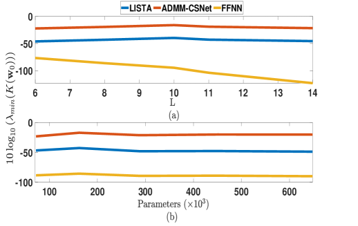
Figure 5: Variation of the minimum eigenvalue of tangent kernel matrix at initialization: (a) With respect to the number of layers. (b) With respect to the network learnable parameters.

V Numerical Experiments

We perform the following simulations to support the proposed theory. For all the simulations in this section, we fix the following for LISTA, ADMM-CSNet, and FFNN: $1.$ Parameters are initialized independently and identically (i.i.d.) from a Gaussian distribution with zero mean and unit variance, i.e., $\mathcal{N}(0,1)$. $2.$ Networks are trained with the aim of minimizing the square loss function (12) using stochastic GD. Note that the theoretical analysis proposed in this work is for GD, however, to address the computation and storage issues, we considered stochastic GD for the numerical analysis. $3.$ Modified soft-plus activation function (refer to IV-A) with $\lambda=1$ is used as the non-linear activation function. $4.$ A batch size of $\frac{T}{5}$ is considered. $5.$ All the simulations are repeated for $10$ trials.

Threshold on $T$: From (31), the choice of $T$ plays a vital role in achieving near-zero training loss. To illustrate this, consider two linear inverse models: $\mathbf{y}_{1}={A}_{1}\mathbf{x}_{1}+\mathbf{e}_{1}$ and $\mathbf{y}_{2}={A}_{2}\mathbf{x}_{2}+\mathbf{e}_{2}$, where $\mathbf{y}_{1}\in\mathbb{R}^{20\times 1}$, $\mathbf{x}_{1}\in\mathbb{R}^{100\times 1}$, $A_{1}\in\mathbb{R}^{20\times 100}$, $\|\mathbf{x}_{1}\|_{0}=2$, $\mathbf{y}_{2}\in\mathbb{R}^{200\times 1}$, $\mathbf{x}_{2}\in\mathbb{R}^{1000\times 1}$, $A_{2}\in\mathbb{R}^{200\times 1000}$, and $\|\mathbf{x}_{2}\|_{0}=10$. Generate synthetic data using a random linear operator matrix, which follows the uniform distribution, and then normalize it to ensure $\|A_{1}\|_{F}=\|A_{2}\|_{F}=10$. Both models are subjected to Gaussian noise $(\mathbf{e}_{1}$ and $\mathbf{e}_{2}$) with a signal-to-noise ratio (SNR) of $10$ dB. Construct an $L$-layer LISTA and ADMM-CSNet with $L=11$. Here, we train LISTA for $30$K epochs and ADMM-CSNet for $40$K epochs. For the first model, we choose $0.12$ and $0.09$ as learning rates for LISTA and ADMM-CSNet, respectively. For the second model, we choose $1.2$ for LISTA and $0.9$ for ADMM-CSNet. Figures 6 and 7 depict the variation of mean square loss/error (MSE) w.r.t. $T$ for both LISTA and ADMM-CSNet, respectively. Note that for a fixed $m$ there exists a threshold (by considering a specific MSE value) on $T$ such that choosing a $T$ value that is less than this threshold leads to near-zero training loss. Moreover, observe that this threshold increases as the network width grows.

For comparison, construct an $L$-layer FFNN, to recover $\mathbf{x}_{1}$ and $\mathbf{x}_{2}$, that has the same number of parameters as that of unfolded, hence, we choose $L=14$. Here, we train the network for $40K$ epochs with a learning rate of $0.04$ for the first model and $0.3$ for the second model. Fig. 8 shows the variation of MSE w.r.t. $T$. From Fig. 8, we can conclude that the threshold for FFNN is lower compared to LISTA and ADMM-CSNet.

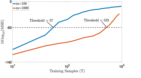
Figure 6: Training loss vs $T$ for LISTA.

Figure 7: Training loss vs $T$ for ADMM-CSNet.

Figure 8: Training loss vs $T$ for FFNN.

Comparison Between Unfolded and Standard Networks: We compare LISTA and ADMM-CSNet with FFNN in terms of parameter efficiency. To demonstrate this, consider the first linear inverse model given in the above simulation. Then, construct LISTA, ADMM-CSNet, and FFNN with a fixed number of parameters and consider $T=30$. Also, consider the same learning rates that are associated with the first model in the above simulation for LISTA, ADMM-CSNet, and FFNN. Here we choose $L=6$ for both LISTA and ADMM-CSNet, and $L=8$ for FFNN, resulting in a total of $72K$ parameters. As shown in Fig. 9, the convergence of training loss to zero is better for LISTA and ADMM-CSNet compared to FFNN. Fig. 9 also shows the training loss convergence of FFNN with $L=11$. Now, FFNN has $102K$ learnable parameters, and its performance is comparable to LISTA for higher epoch values. Therefore, to achieve a better training loss FFNN requires more trainable parameters.

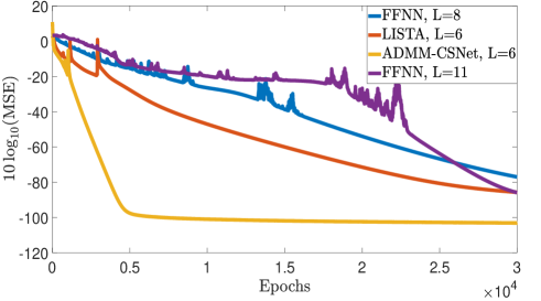
Figure 9: Comparison between LISTA, ADMM-CSNet, and FFNN in terms of the required number of parameters, $P$, for training loss convergence.

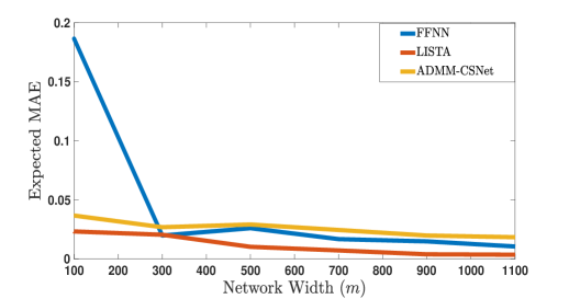
Figure 10: Variation of the expected MAE w.r.t. $m$ for both LISTA and ADMM-CSNet.

Generalization: In this simulation, we show that zero-training error leads to better generalization. To demonstrate this, consider LISTA/ADMM-CSNet/FFNN with a fixed $T$ and observe the variation of the expected mean absolute error (MAE) w.r.t. $m$. If the generalization performance is better, then it is anticipated that the expected MAE reduces as the $m$ increases. Because an increase in $m$ improves the possibility of getting near-zero training loss for a fixed $T$. In Fig. 10, we present the results for LISTA, ADMM-CSNet, and FFNN with $T=100$. Notably, the expected MAE diminishes as $m$ increases, i.e., as the number of parameters grows. Further, it is observed that for this choice of $T$, the training error is near-zero for $m$ values exceeding approximately $300$ for FFNN, and approximately $250$ for both LISTA and ADMM-CSNet. This finding underscores the importance of zero-training error in generalization.

However, it is important to note that the generalization results presented here are preliminary and require a rigorous analysis for more robust conclusions. Because considering a smaller value of $T$ may not yield satisfactory generalization performance. Thus, it is important to find a lower bound on $T$ to optimize both the training process and overall generalization capability, which we consider as a future work of interest.

VI Conclusion

In this work, we provided optimization guarantees for finite-layer LISTA and ADMM-CSNet with smooth nonlinear activation. We begin by deriving the Hessian spectral norm of these unfolded networks. Based on this, we provided conditions on both the network width and the number of training samples, such that the empirical training loss converges to zero as the number of learning epochs increases using the GD approach. Additionally, we showed that LISTA and ADMM-CSNet outperform the standard FFNN in terms of threshold on the number of training samples and parameter efficiency. We provided simulations to support the theoretical findings.

The work presented in this paper is an initial step to understand the theory behind the performance of unfolded networks. While considering certain assumptions, our work raises intriguing questions for future research. For instance, we approximated the soft-threshold activation function with a double-differentiable function formulated using soft-plus. However, it is important to analyze the optimization guarantees without relying on any such approximations. Additionally, we assumed a constant value for $\lambda$ in $\sigma_{\lambda}(\cdot)$. It is interesting to explore the impact of treating $\lambda$ as a learnable parameter. Furthermore, analyzing the changes in the analysis for other loss functions presents an intriguing avenue for further research.

Proof of Theorem 25: The Hessian block ${H}_{s}^{l_{1},l_{2}}$ can be decomposed as given in (35), using the following chain rule:

$$\frac{\partial f_{s}}{\partial\mathbf{w}^{l}}=\frac{\partial\mathbf{g}^{l}}{\partial\mathbf{w}^{l}}\left(\prod_{l^{\prime}=l+1}^{L}\frac{\partial\mathbf{g}^{l}}{\partial\mathbf{g}^{l^{\prime}-1}}\right)\frac{\partial f_{s}}{\partial\mathbf{g}^{L}}.$$

$${H}_{s}^{l_{1},l_{2}}= \frac{\partial^{2}\mathbf{g}^{l_{1}}}{\left(\partial\mathbf{w}^{l_{1}}\right)^{2}}\frac{\partial f_{s}}{\partial\mathbf{g}^{l_{1}}}\mathbb{I}_{l_{1}=l_{2}}+\left(\frac{\partial\mathbf{g}^{l_{1}}}{\partial\mathbf{w}^{l_{1}}}\prod_{l^{\prime}=l_{1}+1}^{l_{2}-1}\frac{\partial\mathbf{g}^{l^{\prime}}}{\partial\mathbf{g}^{l^{\prime}-1}}\right)\frac{\partial^{2}\mathbf{g}^{l_{2}}}{\partial\mathbf{w}^{l_{2}}\partial\mathbf{g}^{l_{2}-1}}$$ (35)

$$\left(\frac{\partial f_{s}}{\partial\mathbf{g}^{l_{2}}}\right)+\sum_{l=l_{2}+1}^{L}\left(\frac{\partial\mathbf{g}^{l_{1}}}{\partial\mathbf{w}^{l_{1}}}\prod_{l^{\prime}=l_{1}+1}^{l-1}\frac{\partial\mathbf{g}^{l^{\prime}}}{\partial\mathbf{g}^{l^{\prime}-1}}\right)\frac{\partial^{2}\mathbf{g}^{l^{\prime}}}{\left(\partial\mathbf{g}^{l^{\prime}-1}\right)^{2}}$$

$$\left(\frac{\partial\mathbf{g}^{l_{2}}}{\partial\mathbf{w}^{l_{2}}}\prod_{l^{\prime}=l_{2}+1}^{l}\frac{\partial\mathbf{g}^{l^{\prime}}}{\partial\mathbf{g}^{l^{\prime}-1}}\right)\left(\frac{\partial f_{s}}{\partial\mathbf{g}^{l}}\right).$$

From (35), the spectral norm of ${H}_{s}^{l_{1},l_{2}}$ can be bounded as

$$\left\|{H}_{s}^{l_{1},l_{2}}\right\|_{2} \leq\left\|\frac{\partial^{2}\mathbf{g}^{l_{1}}}{\left(\partial\mathbf{w}^{\left(l_{1}\right)}\right)^{2}}\right\|_{2,2,1}\left\|\frac{\partial f_{s}}{\partial\mathbf{g}^{l_{1}}}\right\|_{\infty}+L_{\sigma}^{l_{2}-l_{1}-1}\left\|\frac{\partial\mathbf{g}^{l_{1}}}{\partial\mathbf{w}^{l_{1}}}\right\|_{F}$$ (36)

$$\left\|\frac{\partial^{2}\mathbf{g}^{l_{2}}}{\partial\mathbf{w}^{l_{2}}\partial\mathbf{g}^{l_{2}-1}}\right\|_{2,2,1}\left\|\frac{\partial f_{s}}{\partial\mathbf{g}^{l_{2}}}\right\|_{\infty}+\sum_{l=l_{2}+1}^{L}L_{\sigma}^{2l-l_{1}-l_{2}}\left\|\frac{\partial\mathbf{g}^{l_{1}}}{\partial\mathbf{w}^{l_{1}}}\right\|_{F}$$

$$\left\|\frac{\partial^{2}\mathbf{g}^{l}}{\left(\partial\mathbf{g}^{l^{\prime}-1}\right)^{2}}\right\|_{2,2,1}\left\|\frac{\partial\mathbf{g}^{l_{2}}}{\partial\mathbf{w}^{l_{2}}}\right\|_{F}\left\|\frac{\partial f_{s}}{\partial\mathbf{g}^{l}}\right\|_{\infty}.$$

Note that (36) uses the fact that $\left\|\frac{\partial\mathbf{g}^{l^{\prime}}}{\partial\mathbf{g}^{l^{\prime}-1}}\right\|_{F}\leq L_{\sigma}$. By using the notations given in (42) and (43), we get

$$\left\|{H}_{s}^{l_{1},l_{2}}\right\|\leq C_{1}\mathcal{Q}_{2,2,1}\left(f_{s}\right)\mathcal{Q}_{\infty}\left(f_{s}\right),$$

where $C_{1}$ is a constant depend on $L$ and $L_{\sigma}$. ∎

Proof of Lemma 4: For $l=0$, $\|\mathbf{x}^{0}\|\leq\sqrt{m}\|\mathbf{x}^{0}\|_{\infty}\leq\sqrt{m}C_{x}$, $\|\mathbf{z}^{0}\|\leq\sqrt{m}\|\mathbf{z}^{0}\|_{\infty}\leq\sqrt{m}C_{z}$, and $\|\mathbf{u}^{0}\|\leq\sqrt{m}\|\mathbf{u}^{0}\|_{\infty}\leq\sqrt{m}C_{u}$. Whereas for $l=1,2,\dots,L$, we have

$$\left\|\mathbf{x}^{l}\right\| =\left\|\sigma\left(\frac{W_{1}^{l}}{\sqrt{n}}\mathbf{y}+\frac{W_{2}^{l}}{\sqrt{m}}\mathbf{x}^{l-1}\right)\right\|$$

$$\leq L_{\sigma}\left\|\frac{W_{1}^{l}}{\sqrt{n}}\right\|\|\mathbf{y}\|+L_{\sigma}\left\|\frac{W_{2}^{l}}{\sqrt{m}}\right\|\left\|\mathbf{x}^{l-1}\right\|+\sigma(0)$$

$$\leq L_{\sigma}\left(c_{10}+\frac{R_{1}}{\sqrt{n}}\right)\sqrt{n}C_{\mathbf{y}}+L_{\sigma}\left(c_{20}+\frac{R_{2}}{\sqrt{m}}\right)c_{\mathrm{ISTA};x}^{l-1}+\sigma(0)$$

$$=c_{\mathrm{ISTA};\mathbf{x}}^{l}.$$

Here, we used Lemma 3 and $L_{\sigma}$-Lipschitz continuous of the activation function $\sigma(\cdot)$. Similarly,

$$\left\|\mathbf{z}^{l}\right\|=\left\|\sigma\left(\frac{1}{\sqrt{n}}W_{1}^{l}\mathbf{y}+\frac{1}{\sqrt{m}}W_{2}^{l}\left(\mathbf{z}^{l-1}-\mathbf{u}^{l-1}\right)+\mathbf{u}^{l-1}\right)\right\|$$

$$\leq L_{\sigma}\frac{1}{\sqrt{n}}\left\|W_{1}^{l}\right\|\|\mathbf{y}\|+L_{\sigma}\frac{1}{\sqrt{m}}\left\|W_{2}^{l}\right\|\left\|\mathbf{z}^{l-1}\right\|+\frac{1}{\sqrt{m}}L_{\sigma}\left\|W_{2}^{l}\right\|\left\|\mathbf{u}^{l-1}\right\|$$

$$\quad+L_{\sigma}\left\|\mathbf{u}^{l-1}\right\|+\sigma(0)$$

$$\leq L_{\sigma}\left(c_{10}+\frac{R_{1}}{\sqrt{n}}\right)\sqrt{n}C_{y}+L_{\sigma}\left(c_{20}+\frac{R_{2}}{\sqrt{m}}\right)c_{\mathrm{ADMM};\mathbf{z}}^{l-1}$$

$$\quad+L_{\sigma}\left(1+c_{20}+\frac{R_{2}}{\sqrt{m}}\right)c_{\mathrm{ADMM};\mathbf{u}}^{l-1}+\sigma(0)$$

$$=c_{\mathrm{ADMM};\mathbf{z}}^{l}$$

and

$$\left\|\mathbf{u}^{l}\right\|=\left\|\mathbf{u}^{l-1}+\left(\frac{1}{\sqrt{n}}W_{1}^{l}\mathbf{y}+\frac{1}{\sqrt{m}}W_{2}^{l}\left(\mathbf{z}^{l-1}-\mathbf{u}^{l-1}\right)-\mathbf{z}^{l}\right)\right\|$$

$$\leq\left\|\mathbf{u}^{l-1}\right\|+\left\|\frac{1}{\sqrt{n}}W_{1}^{l}\mathbf{y}\right\|+\left\|\frac{1}{\sqrt{m}}W_{2}^{l}\mathbf{z}^{l-1}\right\|+\left\|\frac{1}{\sqrt{m}}W_{2}^{l}\mathbf{u}^{l-1}\right\|+\left\|\mathbf{z}^{l}\right\|$$

$$\leq\left(c_{10}+\frac{R_{1}}{\sqrt{n}}\right)\sqrt{n}C_{y}+\left(c_{20}+\frac{R_{2}}{\sqrt{m}}\right)c_{\mathrm{ADMM};\mathbf{z}}^{l-1}$$

$$\quad+\left(c_{20}+\frac{R_{2}}{\sqrt{m}}+1\right)c_{\mathrm{ADMM};\mathbf{u}}^{l-1}+c_{\mathrm{ADMM};\mathbf{z}}^{l}$$

$$=c_{\mathrm{ADMM};\mathbf{u}}^{l}$$

∎

Proof of Theorem 6: Consider the real symmetric NTK matrix $[K\left(\mathbf{w}_{0}\right)]_{mT\times mT}$. Utilizing the Rayleigh quotient of $K\left(\mathbf{w}_{0}\right)$, we can write the following for any $\mathbf{x}$ such that $\|\mathbf{x}\|_{2}=1$:

$$\lambda_{\min}\left(K\left(\mathbf{w}_{0}\right)\right)\leq\mathbf{x}^{\top}K\left(\mathbf{w}_{0}\right)\mathbf{x}\leq\lambda_{\max}(K\left(\mathbf{w}_{0}\right)).$$

Let $\mathbf{x}$ be a vector having all zeros except the $s^{\text{th}}$ component to be $1$. Thus $\lambda_{\min}(K\left(\mathbf{w}_{0}\right))\leq[K\left(\mathbf{w}_{0}\right)]_{\mathrm{s,s}}$, for any $s\in[mT]$. Assume $s=1$, this implies,

$$\lambda_{\min}\left(K\left(\mathbf{w}_{0}\right)\right)\leq\left\langle\nabla_{\mathbf{w}_{0}}\mathbf{f}_{1},\nabla_{\mathbf{w}_{0}}\mathbf{f}_{1}\right\rangle,$$ (37)

where $\mathbf{f}_{1}$ is the $1^{\text{st}}$ component in the the model output vector $\mathbf{f}$ corresponding to the first training sample. We now aim to compute $\left\langle\nabla_{\mathbf{w}_{0}}\mathbf{f}_{1},\nabla_{\mathbf{w}_{0}}\mathbf{f}_{1}\right\rangle$ for FFNN, LISTA, and ADMM-CSNet.

Consider a one-layer FFNN, then from (34), the $s^{\text{th}}$ component of $\mathbf{f}_{\text{FFNN}}$ is, $\mathbf{f}_{s}=\frac{1}{\sqrt{m}}\sigma\left(\frac{1}{\sqrt{n}}W_{0}^{1}(s,:)\mathbf{y}\right),$ where $W_{0}^{1}(s,:)$ represents the $s^{\text{th}}$ row of $W_{0}^{1}.$ This implies,

$$\left\langle\nabla_{W_{0}^{1}}\mathbf{f}_{s},\nabla_{W_{0}^{1}}\mathbf{f}_{s}\right\rangle=\left[\frac{\sigma^{\prime}(\tilde{\mathbf{x}}_{s}^{1})}{\sqrt{mn}}\right]^{2}\|\mathbf{y}\|^{2}\leq\hat{L}^{2}\hat{y},$$

where $\hat{L}=\frac{L_{\sigma}}{\sqrt{m}},\text{ and }\hat{y}=\frac{\|\mathbf{y}\|^{2}}{n}$. Similarly, for a 2-layered FFNN, we have

$$\left\langle\nabla_{\mathbf{W}_{0}}\mathbf{f}_{s},\nabla_{\mathbf{W}_{0}}\mathbf{f}_{s}\right\rangle =\left\langle\nabla_{W_{0}^{1}}\mathbf{f}_{s},\nabla_{W_{0}^{1}}\mathbf{f}_{s}\right\rangle+\left\langle\nabla_{W_{0}^{2}}\mathbf{f}_{s},\nabla_{W_{0}^{2}}\mathbf{f}_{s}\right\rangle$$

$$\leq(\hat{L}^{2})^{2}\hat{y}\left[\left\|W_{0}^{1}\right\|^{2}+\left\|W_{0}^{2}(s,:)\right\|^{2}\right].$$

Generalizing the above equations, one can derive the upper bound on $\lambda_{0,\text{FFNN}}$ for an L-layer FFNN as

$$\lambda_{0,\text{FFNN}} \leq\text{UB}_{\text{FFNN}}$$ (38)

$$=\hat{L}^{2L}\hat{y}\left[\sum_{i=1}^{L-1}\|\mathbf{v}_{s}^{T}W_{0}^{L}\|^{2}\prod_{j=1,j\neq i}^{L-1}\|W_{0}^{j}\|^{2}+\prod_{j=1}^{L-1}\|W_{0}^{j}\|^{2}\right].$$

Likewise, consider $L=1$, then from (13), the $s^{\text{th}}$ component of $\mathbf{f}_{\text{LISTA}}$ is

$$\mathbf{f}_{s}=\frac{1}{\sqrt{m}}\sigma\left(\frac{1}{\sqrt{n}}W_{10}^{1}(s,:)\mathbf{y}+\frac{1}{\sqrt{m}}W_{20}^{1}(s,:)\mathbf{x}\right).$$

This implies,

$$\left\langle\nabla_{\mathbf{w}_{0}}\mathbf{f}_{s},\nabla_{\mathbf{w}_{0}}\mathbf{f}_{s}\right\rangle =\left\langle\nabla_{W_{10}^{1}}\mathbf{f}_{s},\nabla_{W_{10}^{1}}\mathbf{f}_{s}\right\rangle+\left\langle\nabla_{W_{20}^{1}}\mathbf{f}_{s},\nabla_{W_{20}^{1}}\mathbf{f}_{s}\right\rangle$$

$$\leq\hat{L}^{2}\left[\hat{y}+\hat{x}\right],$$

where $\hat{x}=\frac{\|\mathbf{x}\|^{2}}{m}$. If $L=2$, then the $s^{\text{th}}$ component of $\mathbf{f}_{\text{LISTA}}$ is

$$\left\langle\nabla_{\mathbf{w}_{0}}\mathbf{f}_{s},\nabla_{\mathbf{w}_{0}}\mathbf{f}_{s}\right\rangle =\left\langle\nabla_{W_{10}^{2}}\mathbf{f}_{s},\nabla_{W_{10}^{2}}\mathbf{f}_{s}\right\rangle+\left\langle\nabla_{W_{20}^{2}}\mathbf{f}_{s},\nabla_{W_{20}^{2}}\mathbf{f}_{s}\right\rangle$$

$$+\left\langle\nabla_{W_{10}^{1}}\mathbf{f}_{s},\nabla_{W_{10}^{1}}\mathbf{f}_{s}\right\rangle+\left\langle\nabla_{W_{20}^{1}}\mathbf{f}_{s},\nabla_{W_{20}^{1}}\mathbf{f}_{s}\right\rangle$$

$$\leq\hat{L}^{2}\left[\hat{y}+\hat{L}^{2}\|\tilde{\mathbf{x}}^{(1)}\|^{2}\right]+\hat{L}^{4}\left[\hat{y}+\hat{x}\right]\left\|\mathbf{v}_{s}^{\top}W_{20}^{2}\right\|^{2}.$$

By extending the above equations, we obtain the upper bound on $\lambda_{0,\text{LISTA}}$ for an $L$-layer LISTA as

$$\lambda_{0,\text{LISTA}}\leq\text{UB}_{\text{LISTA}}=\hat{L}^{2}\left(\hat{y}+\hat{x}\right),\ \ \text{for}\ \ L=1$$ (39)

$$\lambda_{0,\text{LISTA}}\leq\text{UB}_{\text{LISTA}}=\hat{L}^{2L}\left(\hat{y}+\hat{x}\right)\|\mathbf{v}_{s}^{T}W_{20}^{L}\|^{2}\prod_{l=2}^{L-1}\|W_{20}^{l}\|^{2}$$

$$+\sum_{k=2}^{L-1}\hat{L}^{2L-2k+2}\left[\hat{y}+\hat{L}^{2}\left\|\tilde{\mathbf{x}}^{(k-1)}\right\|^{2}\right]\|\mathbf{v}_{s}^{T}W_{20}^{L}\|^{2}\prod_{l=k+1}^{L-1}\|W_{20}^{l}\|^{2}$$

$$+\hat{L}^{2}\left[\hat{y}+\hat{L}^{2}\|\tilde{x}^{(L-1)}\|^{2}\right],\text{ for }L>1,$$

where $\hat{L}=\frac{L_{\sigma}}{\sqrt{m}},\ \hat{y}=\frac{\|\mathbf{y}\|^{2}}{n},\ \text{ and }\hat{x}=\frac{\|\mathbf{x}\|^{2}}{m}.$ Repeating the same analysis, one can derive the upper bound on $\lambda_{0,\text{ADMM-CSNet}}$ of an $L$-layer ADMM-CSNet as

$$\lambda_{0,\text{ADMM-CSNet}}\leq\text{UB}_{\text{ADMM-CSNet}}=\hat{L}^{2}\left[\hat{y}+\hat{a}^{(L-1)}\right]$$ (40)

$$+\sum_{k=1}^{L-1}\hat{L}^{2L-2k+2}\left[\hat{y}+\hat{a}^{(k-1)}\right]\|\mathbf{v}_{s}^{T}W_{20}^{L}\|^{2}\prod_{l=k+1}^{L-1}\|W_{20}^{l}\|^{2},$$

where $\hat{a}^{(l)}=\frac{\|\mathbf{z}^{(l)}-\mathbf{u}^{(l)}\|^{2}}{m},\ \forall l\in[L-1]\cup\{0\}$. ∎

Supporting Material: Optimization Guarantees of Unfolded ISTA and ADMM Networks With Smooth Soft-Thresholding

From Theorem 3, the Hessian spectral norm, $\|\mathbf{H}\|_{2}$, of an $L$-layer unfolded ISTA (ADMM) network is bounded as

$$\|\mathbf{H}\|_{2} \leq\sum_{s,l_{1},l_{2}}C_{1}\mathcal{Q}_{2,2,1}\left(f_{s}\right)\mathcal{Q}_{\infty}\left(f_{s}\right)$$ (41)

$$\leq\sum_{s=1}^{m}C\mathcal{Q}_{2,2,1}\left(f_{s}\right)\mathcal{Q}_{\infty}\left(f_{s}\right),$$

where the constant $C_{1}$ depends on $L$ and $L_{\sigma}$, $C=L^{2}C_{1}$,

$$\mathcal{Q}_{\infty}\left(f_{s}\right)=\max_{1\leq l\leq L}\left\{\left\|\frac{\partial f_{s}}{\partial\mathbf{g}^{l}}\right\|_{\infty}\right\}\text{ and}$$ (42)

$$\mathcal{Q}_{2,2,1}\left(f_{s}\right)=\max_{1\leq l_{1}\leq l_{2}<l_{3}\leq L}\Bigg{\{}\left\|\frac{\partial^{2}\mathbf{g}^{l_{1}}}{\left(\partial\mathbf{w}^{l_{1}}\right)^{2}}\right\|_{2,2,1},\left\|\frac{\partial\mathbf{g}^{l_{1}}}{\partial\mathbf{w}^{l_{1}}}\right\|\left\|\frac{\partial^{2}\mathbf{g}^{l_{2}}}{\partial\mathbf{g}^{\left(l_{2}-1\right)}\partial\mathbf{w}^{l_{2}}}\right\|_{2,2,1},\left\|\frac{\partial\mathbf{g}^{l_{1}}}{\partial\mathbf{w}^{l_{1}}}\right\|\left\|\frac{\partial\mathbf{g}^{l_{2}}}{\partial\mathbf{w}^{l_{2}}}\right\|\left\|\frac{\partial^{2}\mathbf{g}^{l_{3}}}{\left(\partial\mathbf{g}^{l_{3}-1}\right)^{2}}\right\|_{2,2,1}\Bigg{\}}.$$ (43)

Note that $\mathbf{g}^{l}=\mathbf{x}^{l}$ for LISTA and $\mathbf{g}^{l}=\mathbf{z}^{l}$ for ADMM-CSNet.

Appendix A Proof of Theorem $4$

Theorem $4$ aims to provide bounds on $\mathcal{Q}_{\infty}\left(f_{s}\right)$ and $\mathcal{Q}_{2,2,1}\left(f_{s}\right)$. The proof of this theorem has been divided into two parts: First, we prove the bound on $Q_{2,2,1}$ in sub-sections A-A and A-B, respectively. Then, we prove the bound on $Q_{\infty}$ in sub-sections A-C and A-D, respectively. Here we denote $\|\cdot\|$ as $l_{2}$-norm for vectors and spectral norm for matrices. We also denote $\|\cdot\|_{F}$ as the Frobenious norm of matrices.

A-A Bound on $Q_{2,2,1}$ For LISTA Network

Consider an L-layer unfolded ISTA network with output

$$\mathbf{f} =\frac{1}{\sqrt{m}}\mathbf{x}^{L},\text{ where }$$ (44)

$$\mathbf{x}^{l} =\sigma(\tilde{\mathbf{x}}^{l})=\sigma\left(\frac{W_{1}^{l}}{\sqrt{n}}\mathbf{y}+\frac{W_{2}^{l}}{\sqrt{m}}\mathbf{x}^{l-1}\right)\ \in\mathbb{R}^{m},\ l\in[L].$$

Now the first derivatives of $\mathbf{x}^{l}$ are

$$\left(\frac{\partial\mathbf{x}^{l}}{\partial\mathbf{x}^{l-1}}\right)_{i,j}=\frac{1}{\sqrt{m}}\sigma^{\prime}\left(\tilde{\mathbf{x}}_{i}^{l}\right)\left(W_{2}\right)_{i,j}^{l},\left(\frac{\partial\mathbf{x}^{l}}{\partial W_{1}^{l}}\right)_{i,jj^{\prime}}=\frac{1}{\sqrt{n}}\sigma^{\prime}\left(\tilde{\mathbf{x}}_{i}^{l}\right)\mathbf{y}_{j^{\prime}}\mathbb{I}_{i=j},\left(\frac{\partial\mathbf{x}^{l}}{\partial W_{2}^{l}}\right)_{i,jj^{\prime}}=\frac{1}{\sqrt{m}}\sigma^{\prime}\left(\tilde{\mathbf{x}}_{i}^{l}\right)\mathbf{x}_{j^{\prime}}^{l-1}\mathbb{I}_{i=j}.$$

By the definition of spectral norm, $\|A\|_{2}=\sup_{\|\mathbf{v}\|_{2}=1}\|A\mathbf{v}\|_{2}$, we have

$$\left\|\frac{\partial\mathbf{x}^{l}}{\partial W_{1}^{l}}\right\|^{2}=\sup_{\|V\|_{F}=1}\frac{1}{n}\sum_{i}\left(\sum_{j,j^{\prime}}\sigma^{\prime}\left(\tilde{\mathbf{x}}_{i}^{l}\right)\mathbf{y}_{j^{\prime}}V_{j,j^{\prime}}\mathbb{I}_{i=j}\right)^{2}=\sup_{\|V\|_{F}=1}\frac{1}{n}\left\|\Sigma^{\prime l}V\mathbf{y}\right\|^{2}\leq\frac{1}{n}\left\|\Sigma^{\prime l}\right\|^{2}\|\mathbf{y}\|^{2}\leq L_{\sigma}^{2}C_{y}^{2}=O(1),$$

where $\Sigma^{\prime l}$ is a diagonal matrix with the diagonal entry $(\Sigma^{\prime l})_{ii}=\sigma^{\prime}\left(\tilde{\mathbf{x}}_{i}^{l}\right)$. Similarly,

$$\left\|\frac{\partial\mathbf{x}^{l}}{\partial W_{2}^{l}}\right\|^{2} =\sup_{\|V\|_{F}=1}\frac{1}{m}\sum_{i}\left(\sum_{j,j^{\prime}}\sigma^{\prime}\left(\tilde{\mathbf{x}}_{i}^{l}\right)\mathbf{x}_{j^{\prime}}^{l-1}V_{j,j^{\prime}}\mathbb{I}_{i=j}\right)^{2}=\sup_{\|V\|_{F}=1}\frac{1}{m}\left\|\Sigma^{\prime l}V\mathbf{x}^{l-1}\right\|^{2}$$

$$\leq\frac{1}{m}L_{\sigma}^{2}\left\|\mathbf{x}^{l-1}\right\|^{2}\leq\frac{1}{m}L_{\sigma}^{2}\left(c_{\text{ISTA };\mathbf{x}}^{l-1}\right)^{2}=O(1).$$

Here we used $\left(c_{\text{ISTA };\mathbf{x}}^{l-1}\right)=O(\sqrt{m})$ from lemma (4).

$$\left\|\frac{\partial\mathbf{x}^{l}}{\partial W^{l}}\right\|=\left\|\left[\frac{\partial\mathbf{x}^{l}}{\partial W_{1}^{l}}\quad\frac{\partial\mathbf{x}^{l}}{\partial W_{2}^{l}}\right]\right\|\leq\left\|\frac{\partial\mathbf{x}^{l}}{\partial W_{1}^{l}}\right\|+\left\|\frac{\partial\mathbf{x}^{l}}{\partial W_{2}^{l}}\right\|=O(1)+O(1)=O(1).$$ (45)

The second-order derivatives of the vector-valued layer function $\mathbf{x}^{l}$, which are order 3 tensors, have the following expressions:

$$\left(\frac{\partial^{2}\mathbf{x}^{l}}{\left(\partial\mathbf{x}^{l-1}\right)^{2}}\right)_{i,j,k}=\frac{1}{m}\sigma^{\prime\prime}\left(\tilde{\mathbf{x}}_{i}^{l}\right)\left(W_{2}\right)_{i,j}^{l}\left(W_{2}\right)_{i,k}^{l};\quad\left(\frac{\partial^{2}\mathbf{x}^{l}}{\partial\mathbf{x}^{l-1}\partial W_{2}^{l}}\right)_{i,j,kk^{\prime}}=\frac{1}{m}\sigma^{\prime\prime}\left(\tilde{\mathbf{x}}_{i}^{l}\right)\left(W_{2}\right)_{i,j}^{l}\mathbf{x}_{k^{\prime}}^{l-1}\mathbb{I}_{i=k};$$

$$\left(\frac{\partial^{2}\mathbf{x}^{l}}{\partial\mathbf{x}^{l-1}\partial W_{1}^{l}}\right)_{i,j,kk^{\prime}}=\frac{1}{\sqrt{mn}}\sigma^{\prime\prime}\left(\tilde{\mathbf{x}}_{i}^{l}\right)\left(W_{2}\right)_{i,j}^{l}\mathbf{y}_{k^{\prime}}\mathbb{I}_{i=k};\quad\left(\frac{\partial^{2}\mathbf{x}^{l}}{\left(\partial W_{2}^{l}\right)^{2}}\right)_{i,jj^{\prime},kk^{\prime}}=\frac{1}{m}\sigma^{\prime\prime}\left(\tilde{\mathbf{x}}_{i}^{l}\right)\mathbf{x}_{j^{\prime}}^{l-1}\mathbf{x}_{k^{\prime}}^{l-1}\mathbb{I}_{i=k=j};$$

$$\left(\frac{\partial^{2}\mathbf{x}^{l}}{\partial W_{2}^{l}\partial W_{1}^{l}}\right)_{i,jj^{\prime},kk^{\prime}}=\frac{1}{\sqrt{mn}}\sigma^{\prime\prime}\left(\tilde{\mathbf{x}}_{i}^{l}\right)\mathbf{x}_{j^{\prime}}^{l-1}\mathbf{y}_{k^{\prime}}\mathbb{I}_{i=k=j};\quad\left(\frac{\partial^{2}\mathbf{x}^{l}}{\left(\partial W_{1}^{l}\right)^{2}}\right)_{i,jj^{\prime},kk^{\prime}}=\frac{1}{n}\sigma^{\prime\prime}\left(\tilde{\mathbf{x}}_{i}^{l}\right)\mathbf{y}_{j^{\prime}}\mathbf{y}_{k^{\prime}}\mathbb{I}_{i=k=j};$$

$$\left\|\frac{\partial^{2}\mathbf{x}^{l}}{\left(\partial\mathbf{x}^{l-1}\right)^{2}}\right\|_{2,2,1}= \sup_{\left\|\mathbf{v}_{1}\right\|=\left\|\mathbf{v}_{2}\right\|=1}\frac{1}{m}\sum_{i=1}^{m}\left|\sigma^{\prime\prime}\left(\tilde{\mathbf{x}}_{i}^{l}\right)\left(W_{2}^{l}\mathbf{v}_{1}\right)_{i}\left(W_{2}^{l}\mathbf{v}_{2}\right)_{i}\right|\leq\sup_{\left\|\mathbf{v}_{1}\right\|=\left\|\mathbf{v}_{2}\right\|=1}\frac{1}{m}\beta_{\sigma}\sum_{i=1}^{m}\left|\left(W_{2}^{l}\mathbf{v}_{1}\right)_{i}\left(W_{2}^{l}\mathbf{v}_{2}\right)_{i}\right|$$ (46)

$$\leq\sup_{\left\|\mathbf{v}_{1}\right\|=\left\|\mathbf{v}_{2}\right\|=1}\frac{1}{2m}\beta_{\sigma}\sum_{i=1}^{m}\left(W_{2}^{l}\mathbf{v}_{1}\right)_{i}^{2}+\left(W_{2}^{l}\mathbf{v}_{2}\right)_{i}^{2}\leq\sup_{\left\|\mathbf{v}_{1}\right\|=\left\|\mathbf{v}_{2}\right\|=1}\frac{1}{2m}\beta_{\sigma}\left(\left\|W_{2}^{l}\mathbf{v}_{1}\right\|^{2}+\left\|W_{2}^{l}\mathbf{v}_{2}\right\|^{2}\right)$$

$$\leq\frac{1}{2m}\beta_{\sigma}\left(\left\|W_{2}^{l}\right\|_{2}^{2}+\left\|W_{2}^{l}\right\|_{2}^{2}\right)\leq\beta_{\sigma}\left(c_{20}+\frac{R_{2}}{\sqrt{m}}\right)^{2}=O(1),$$

$$\left\|\frac{\partial^{2}\mathbf{x}^{l}}{\partial\mathbf{x}^{l-1}\partial W_{2}^{l}}\right\|_{2,2,1} =\sup_{\left\|\mathbf{v}_{1}\right\|=\left\|V_{2}\right\|_{F}=1}\frac{1}{m}\sum_{i=1}^{m}\left|\sigma^{\prime\prime}\left(\tilde{\mathbf{x}}_{i}^{l}\right)\left(W_{2}^{l}\mathbf{v}_{1}\right)_{i}\left(V_{2}\mathbf{x}^{l-1}\right)_{i}\right|\leq\sup_{\left\|\mathbf{v}_{1}\right\|=\left\|V_{2}\right\|_{F}=1}\frac{1}{2m}\beta_{\sigma}\left(\left\|W_{2}^{l}\mathbf{v}_{1}\right\|^{2}+\left\|V_{2}\mathbf{x}^{l-1}\right\|^{2}\right)$$

$$\leq\frac{1}{2m}\beta_{\sigma}\left(\left\|W_{2}^{l}\right\|^{2}+\left\|\mathbf{x}^{l-1}\right\|^{2}\right)\leq\frac{\beta_{\sigma}}{2m}\left(c_{20}\sqrt{m}+R_{2}\right)^{2}+\frac{\beta_{\sigma}}{2m}\left(c_{\text{ISTA };\mathbf{x}}^{l-1}\right)^{2}=O(1),$$

$$\left\|\frac{\partial^{2}\mathbf{x}^{l}}{\partial\mathbf{x}^{l-1}\partial W_{1}^{l}}\right\|_{2,2,1} =\sup_{\left\|\mathbf{v}_{1}\right\|=\left\|V_{2}\right\|_{F}=1}\frac{1}{\sqrt{mn}}\sum_{i=1}^{m}\left|\sigma^{\prime\prime}\left(\tilde{\mathbf{x}}_{i}^{l}\right)\left(W_{2}^{l}\mathbf{v}_{1}\right)_{i}\left(V_{2}\mathbf{y}\right)_{i}\right|\leq\sup_{\left\|\mathbf{v}_{1}\right\|=\left\|V_{2}\right\|_{F}=1}\frac{1}{2\sqrt{mn}}\beta_{\sigma}\left(\left\|W_{2}^{l}\mathbf{v}_{1}\right\|^{2}+\left\|V_{2}\mathbf{y}\right\|^{2}\right)$$

$$\leq\frac{1}{2\sqrt{mn}}\beta_{\sigma}\left(\left\|W_{2}^{l}\right\|^{2}+\|\mathbf{y}\|^{2}\right)\leq\sqrt{\frac{m}{4n}}\beta_{\sigma}\left(c_{20}+\frac{R_{2}}{\sqrt{m}}\right)^{2}+\sqrt{\frac{n}{4m}}\beta_{\sigma}C_{y}^{2}=O(1),$$

$$\left\|\frac{\partial^{2}\mathbf{x}^{l}}{\left(\partial W_{2}^{l}\right)^{2}}\right\|_{2,2,1} =\sup_{\left\|V_{1}\right\|_{F}=\left\|V_{2}\right\|_{F}=1}\frac{1}{m}\sum_{i=1}^{m}\left|\sigma^{\prime\prime}\left(\tilde{\mathbf{x}}_{i}^{l}\right)\left(V_{1}\mathbf{x}^{l-1}\right)_{i}\left(V_{2}\mathbf{x}^{l-1}\right)_{i}\right|\leq\sup_{\left\|V_{1}\right\|_{F}=\left\|V_{2}\right\|_{F}=1}\frac{1}{2m}\beta_{\sigma}\left(\left\|V_{1}\mathbf{x}^{l-1}\right\|^{2}+\left\|V_{2}\mathbf{x}^{l-1}\right\|^{2}\right)$$

$$\leq\frac{1}{2m}\beta_{\sigma}\left(\left\|\mathbf{x}^{l-1}\right\|^{2}+\left\|\mathbf{x}^{l-1}\right\|^{2}\right)\leq\frac{1}{m}\beta_{\sigma}\left(c_{\mathrm{ISTA};\mathbf{x}}^{l-1}\right)^{2}=O(1),$$

$$\left\|\frac{\partial^{2}\mathbf{x}^{l}}{\partial W_{2}^{l}\partial W_{1}^{l}}\right\|_{2,2,1} =\sup_{\left\|V_{1}\right\|_{F}=\left\|V_{2}\right\|_{F}=1}\frac{1}{\sqrt{mn}}\sum_{i=1}^{m}\left|\sigma^{\prime\prime}\left(\tilde{\mathbf{x}}_{i}^{l}\right)\left(V_{1}\mathbf{x}_{i}^{l-1}\right)_{i}\left(V_{2}\mathbf{y}\right)_{i}\right|\leq\sup_{\left\|V_{1}\right\|_{F}=\left\|V_{2}\right\|_{F}=1}\frac{1}{2\sqrt{mn}}\beta_{\sigma}\left(\left\|V_{1}\mathbf{x}^{l-1}\right\|^{2}+\left\|V_{2}\mathbf{y}\right\|^{2}\right)$$

$$\leq\frac{1}{2\sqrt{mn}}\beta_{\sigma}\left(\left\|\mathbf{x}^{l-1}\right\|^{2}+\|\mathbf{y}\|^{2}\right)\leq\frac{\beta_{\sigma}}{2\sqrt{mn}}\left(c_{\text{ISTA;$\mathbf{x}$ }}^{l-1}\right)^{2}+\sqrt{\frac{n}{4m}}\beta_{\sigma}C_{y}^{2}=O(1),$$

$$\left\|\frac{\partial^{2}\mathbf{x}^{l}}{\left(\partial W_{1}^{l}\right)^{2}}\right\|_{2,2,1} =\sup_{\left\|V_{1}\right\|_{F}=\left\|V_{2}\right\|_{F}=1}\frac{1}{n}\sum_{i=1}^{m}\left|\sigma^{\prime\prime}\left(\tilde{\mathbf{x}}_{i}^{l}\right)\left(V_{1}\mathbf{y}\right)_{i}\left(V_{2}\mathbf{y}\right)_{i}\right|\leq\sup_{\left\|V_{1}\right\|_{F}=\left\|V_{2}\right\|_{F}=1}\frac{1}{2n}\beta_{\sigma}\left(\left\|V_{1}\mathbf{y}\right\|^{2}+\left\|V_{2}\mathbf{y}\right\|^{2}\right)$$

$$\leq\frac{1}{2n}\beta_{\sigma}\left(\|\mathbf{y}\|^{2}+\|\mathbf{y}\|^{2}\right)=\beta_{\sigma}C_{y}^{2}=O(1),$$

$$\left\|\frac{\partial^{2}\mathbf{x}^{l}}{\partial\mathbf{x}^{l-1}\partial W^{l}}\right\|_{2,2,1} =\left\|\left[\begin{array}[]{ll}\frac{\partial^{2}\mathbf{x}^{l}}{\partial\mathbf{x}^{l-1}\partial W_{1}^{l}}&\frac{\partial^{2}\mathbf{x}^{l}}{\partial\mathbf{x}^{l-1}\partial W_{2}^{l}}\end{array}\right]\right\|_{2,2,1}\leq\left\|\frac{\partial^{2}\mathbf{x}^{l}}{\partial\mathbf{x}^{l-1}\partial W_{1}^{l}}\right\|_{2,2,1}+\left\|\frac{\partial^{2}\mathbf{x}^{l}}{\partial\mathbf{x}^{l-1}\partial W_{2}^{l}}\right\|_{2,2,1}$$ (47)

$$=O(1)+O(1)=O(1),$$

$$\left\|\frac{\partial^{2}\mathbf{x}^{l}}{\left(\partial W^{l}\right)^{2}}\right\|_{2,2,1} =\left\|\left[\begin{array}[]{cc}\partial^{2}\mathbf{x}^{l}/\left(\partial W_{1}^{l}\right)^{2}&\partial^{2}\mathbf{x}^{l}/\partial W_{1}^{l}\partial W_{2}^{l}\\ \partial^{2}\mathbf{x}^{l}/\partial W_{1}^{l}\partial W_{2}^{l}&\partial^{2}\mathbf{x}^{l}/\left(\partial W_{2}^{l}\right)^{2}\end{array}\right]\right\|_{2,2,1}\leq\left\|\frac{\partial^{2}\mathbf{x}^{l}}{\left(\partial W_{1}^{l}\right)^{2}}\right\|_{2,2,1}+2\left\|\frac{\partial^{2}\mathbf{x}^{l}}{\partial W_{1}^{l}\partial W_{2}^{l}}\right\|_{2,2,1}+\left\|\frac{\partial^{2}\mathbf{x}^{l}}{\left(\partial W_{2}^{l}\right)^{2}}\right\|_{2,2,1}$$ (48)

$$=O(1)+O(1)+O(1)=O(1).$$

Therefore, by using (45), (46), (47), and (48), we get $\mathcal{Q}_{2,2,1}\left(f_{s}\right)=O(1)$, for all $s\in[m]$.

A-B Bound on $Q_{2,2,1}$ For ADMM-CSNet

Consider an L-layered ADMM-CSNet as

$$\mathbf{f} =\frac{1}{\sqrt{m}}\mathbf{z}^{L};$$ (49)

$$\mathbf{z}^{l} =\sigma\left(\tilde{\mathbf{z}}^{l}\right)=\sigma\left(\mathbf{x}^{l}+\mathbf{u}^{l-1}\right),$$

$$\mathbf{x}^{l} =\frac{1}{\sqrt{n}}W_{1}^{l}\mathbf{y}+\frac{1}{\sqrt{m}}W_{2}^{l}\left(\mathbf{z}^{l-1}-\mathbf{u}^{l-1}\right),$$

$$\mathbf{u}^{l} =\mathbf{u}^{l-1}+\left(\mathbf{x}^{l}-\mathbf{z}^{l}\right).$$

where f is the output of the network. Now the first derivatives of $\mathbf{z}^{l}$ are

$$\left(\frac{\partial\mathbf{z}^{l}}{\partial\mathbf{z}^{l-1}}\right)_{i,j}=\left(\frac{\partial\mathbf{z}^{l}}{\partial\mathbf{z}^{l-1}}\right)_{i,j}+\left(\frac{\partial\mathbf{z}^{l}}{\partial\mathbf{u}^{l-1}}\frac{\partial\mathbf{u}^{l-1}}{\partial\mathbf{z}^{l-1}}\right)_{i,j}=\sigma^{\prime}\left(\tilde{\mathbf{z}}_{i}^{l}\right)\left(\frac{2}{\sqrt{m}}W_{2}^{l}-I\right)_{i,j};$$

$$\left(\frac{\partial\mathbf{z}^{l}}{\partial W_{1}^{l}}\right)_{i,jj^{\prime}}=\frac{1}{\sqrt{n}}\sigma^{\prime}\left(\tilde{\mathbf{z}}_{i}^{l}\right)\mathbf{y}_{j^{\prime}}\mathbb{I}_{i=j};\left(\frac{\partial\mathbf{z}^{l}}{\partial W_{2}^{l}}\right)_{i,jj^{\prime}}=\frac{1}{\sqrt{m}}\sigma^{\prime}\left(\tilde{\mathbf{z}}_{i}^{l}\right)(\mathbf{z}^{l-1}-\mathbf{u}^{l-1})_{j^{\prime}}\mathbb{I}_{i=j}.$$

Now, we have

$$\left\|\frac{\partial\mathbf{z}^{l}}{\partial W_{1}^{l}}\right\|_{2}^{2} =\sup_{\|V\|_{F}=1}\frac{1}{n}\sum_{i=1}^{m}\left(\sum_{j,j^{\prime}}\sigma^{\prime}\left(\tilde{\mathbf{z}}_{i}^{l}\right)\mathbf{y}_{j^{\prime}}\mathbb{I}_{i=j}V_{jj^{\prime}}\right)^{2}=\sup_{\|V\|_{F}=1}\frac{1}{n}\left\|\Sigma^{\prime l}V\mathbf{y}\right\|^{2}\leq\frac{1}{n}\left\|\Sigma^{\prime l}\right\|^{2}\|\mathbf{y}\|^{2}\leq L_{\sigma}^{2}C_{y}^{2}=O(1),$$

where $\Sigma^{\prime l}$ is a diagonal matrix with the diagonal entry $(\Sigma^{\prime l})_{ii}=\sigma^{\prime}\left(\tilde{\mathbf{z}}_{i}^{l}\right)$.

$$\left\|\frac{\partial\mathbf{z}^{l}}{\partial W_{2}^{l}}\right\|_{2}^{2} =\sup_{\|V\|_{F}=1}\frac{1}{m}\sum_{i=1}^{m}\left(\sum_{j,j^{\prime}}\sigma^{\prime}\left(\tilde{\mathbf{z}}_{i}^{l}\right)(\mathbf{z}^{l-1}-\mathbf{u}^{l-1})_{j^{\prime}}\mathbb{I}_{i=j}V_{jj^{\prime}}\right)^{2}=\sup_{\|V\|_{F}=1}\frac{1}{m}\left\|\Sigma^{\prime l}V(\mathbf{z}^{l-1}-\mathbf{u}^{l-1})\right\|^{2}$$

$$\leq\frac{1}{m}\left\|\Sigma^{\prime l}\right\|^{2}\left\|\mathbf{z}^{l-1}\right\|^{2}+\frac{1}{m}\left\|\Sigma^{\prime l}\right\|^{2}\left\|\mathbf{u}^{l-1}\right\|^{2}\leq\frac{1}{m}L_{\sigma}^{2}\left(\left(c_{\mathrm{ADMM};\mathbf{z}}^{l-1}\right)^{2}+\left(c_{\mathrm{ADMM};\mathbf{u}}^{l-1}\right)^{2}\right)=O(1).$$

From lemma (4) we used $\left(c_{\mathrm{ADMM};\mathbf{z}}^{l-1}\right)=O(\sqrt{m})$ and $\left(c_{\mathrm{ADMM};\mathbf{u}}^{l-1}\right)=O(\sqrt{m})$. Therefore

$$\left\|\frac{\partial\mathbf{z}^{l}}{\partial W^{l}}\right\| =\left\|\left[\frac{\partial\mathbf{z}^{l}}{\partial W_{1}^{l}}\quad\frac{\partial\mathbf{z}^{l}}{\partial W_{2}^{l}}\right]\right\|\leq\left\|\frac{\partial\mathbf{z}^{l}}{\partial W_{1}^{l}}\right\|+\left\|\frac{\partial\mathbf{z}^{l}}{\partial W_{2}^{l}}\right\|=O(1)+O(1)=O(1).$$ (50)

The second derivatives of the vector-valued layer function $\mathbf{z}^{l}$, which are order 3 tensors, have the following expressions:

$$\left(\frac{\partial^{2}\mathbf{z}^{l}}{\left(\partial\mathbf{z}^{l-1}\right)^{2}}\right)_{i,j,k}=\sigma^{\prime\prime}\left(\tilde{\mathbf{z}}_{i}^{l}\right)\left(\frac{2}{\sqrt{m}}W_{2}^{l}-I\right)_{i,j}\left(\frac{2}{\sqrt{m}}W_{2}^{l}-I\right)_{i,k};$$ (51)

$$\left(\frac{\partial^{2}\mathbf{z}^{l}}{\partial\mathbf{z}^{l-1}\partial W_{2}^{l}}\right)_{i,j,kk^{\prime}}=\frac{1}{\sqrt{m}}\sigma^{\prime\prime}\left(\tilde{\mathbf{z}}_{i}^{l}\right)\left(\frac{2}{\sqrt{m}}W_{2}^{l}-I\right)_{ij}(\mathbf{z}^{l-1}-\mathbf{u}^{l-1})_{k^{\prime}}\mathbb{I}_{i=k}+\frac{2}{\sqrt{m}}\sigma^{\prime}\left(\tilde{\mathbf{z}}_{i}^{l}\right)\mathbb{I}_{i=k}\mathbb{I}_{j=k^{\prime}};$$

$$\left(\frac{\partial^{2}\mathbf{z}^{l}}{\partial\mathbf{z}^{l-1}\partial W_{1}^{l}}\right)_{i,j,kk^{\prime}}=\frac{1}{\sqrt{m}}\sigma^{\prime\prime}\left(\tilde{\mathbf{z}}_{i}^{l}\right)\left(\frac{2}{\sqrt{m}}W_{2}^{l}-I\right)_{ij}\mathbf{y}_{k^{\prime}}\mathbb{I}_{i=k};$$

$$\left(\frac{\partial^{2}\mathbf{z}^{l}}{\left(\partial W_{2}^{l}\right)^{2}}\right)_{i,jj^{\prime},kk^{\prime}}=\frac{1}{m}\sigma^{\prime\prime}\left(\tilde{\mathbf{z}}_{i}^{l}\right)(\mathbf{z}^{l-1}-\mathbf{u}^{l-1})_{j^{\prime}}(\mathbf{z}^{l-1}-\mathbf{u}^{l-1})_{k^{\prime}}\mathbb{I}_{i=k=j};$$

$$\left(\frac{\partial^{2}\mathbf{z}^{l}}{\partial W_{2}^{l}\partial W_{1}^{l}}\right)_{i,jj^{\prime},kk^{\prime}}=\frac{1}{\sqrt{mn}}\sigma^{\prime\prime}\left(\tilde{\mathbf{z}}_{i}^{l}\right)(\mathbf{z}^{l-1}-\mathbf{u}^{l-1})_{j^{\prime}}\mathbf{y}_{k^{\prime}}\mathbb{I}_{i=k=j};$$

$$\left(\frac{\partial^{2}\mathbf{z}^{l}}{\left(\partial W_{1}^{l}\right)^{2}}\right)_{i,jj^{\prime},kk^{\prime}}=\frac{1}{n}\sigma^{\prime\prime}\left(\tilde{\mathbf{z}}_{i}^{l}\right)\mathbf{y}_{j^{\prime}}\mathbf{y}_{k^{\prime}}\mathbb{I}_{i=k=j};$$

$$\left\|\frac{\partial^{2}\mathbf{z}^{l}}{\left(\partial\mathbf{z}^{l-1}\right)^{2}}\right\|_{2,2,1} =\sup_{\left\|\mathbf{v}_{1}\right\|=\left\|\mathbf{v}_{2}\right\|=1}\sum_{i=1}^{m}\left|\sigma^{\prime\prime}\left(\tilde{\mathbf{z}}_{i}^{l}\right)\left(\left(\frac{2}{\sqrt{m}}W_{2}^{l}-I\right)\mathbf{v}_{1}\right)_{i}\left(\left(\frac{2}{\sqrt{m}}W_{2}^{l}-I\right)\mathbf{v}_{2}\right)_{i}\right|$$ (52)

$$\leq\sup_{\left\|\mathbf{v}_{1}\right\|=\left\|\mathbf{v}_{2}\right\|=1}\beta_{\sigma}\sum_{i=1}^{m}\left|\left(\left(\frac{2}{\sqrt{m}}W_{2}^{l}-I\right)\mathbf{v}_{1}\right)_{i}\left(\left(\frac{2}{\sqrt{m}}W_{2}^{l}-I\right)\mathbf{v}_{2}\right)_{i}\right|$$

$$\leq\sup_{\left\|\mathbf{v}_{1}\right\|=\left\|\mathbf{v}_{2}\right\|=1}\frac{1}{2}\beta_{\sigma}\sum_{i=1}^{m}\left(\left(\frac{2}{\sqrt{m}}W_{2}^{l}-I\right)\mathbf{v}_{1}\right)_{i}^{2}+\left(\left(\frac{2}{\sqrt{m}}W_{2}^{l}-I\right)^{2}\right)_{i}$$

$$\leq\sup_{\left\|\mathbf{v}_{1}\right\|=\left\|\mathbf{v}_{2}\right\|=1}\frac{1}{2}\beta_{\sigma}\left(\left\|\frac{2}{\sqrt{m}}W_{2}^{l}\mathbf{v}_{1}-\mathbf{v}_{1}\right\|^{2}+\left\|\frac{2}{\sqrt{m}}W_{2}^{l}\mathbf{v}_{2}-\mathbf{v}_{2}\right\|^{2}\right)$$

$$\leq\beta_{\sigma}\left(\left\|\frac{2}{\sqrt{m}}W_{2}^{l}\right\|^{2}+1^{2}\right)\leq\beta_{\sigma}+4\beta_{\sigma}\frac{\left(c_{20}\sqrt{m}+R_{2}\right)^{2}}{m}=O(1),$$

$$\left\|\frac{\partial^{2}\mathbf{z}^{l}}{\partial\mathbf{z}^{l-1}\partial W_{2}^{l}}\right\|_{2,2,1} =\sup_{\left\|\mathbf{v}_{1}\right\|=\left\|V_{2}\right\|_{F}=1}\sum_{i=1}^{m}\left|\frac{1}{m}\sigma^{\prime\prime}\left(\tilde{\mathbf{z}}_{i}^{l}\right)\left(\left(2W_{2}^{l}-\sqrt{m}I\right)\mathbf{v}_{1}\right)_{i}\left(V_{2}(\mathbf{z}^{l-1}-\mathbf{u}^{l-1})\right)_{i}+\frac{2}{\sqrt{m}}\sigma^{\prime}\left(\tilde{\mathbf{z}}_{i}^{l}\right)\left(V_{2}\mathbf{v}_{1}\right)_{i}\right|$$

$$\leq\sup_{\left\|\mathbf{v}_{1}\right\|=\left\|V_{2}\right\|_{F}=1}\frac{1}{2m}\beta_{\sigma}\left(\left\|2W_{2}^{l}\mathbf{v}_{1}-\sqrt{m}\mathbf{v}_{1}\right\|^{2}+\left\|V_{2}\mathbf{z}^{l-1}-V_{2}\mathbf{u}^{l-1}\right\|^{2}\right)+\frac{2}{\sqrt{m}}\left\|\Sigma^{\prime l}\right\|\left\|\mathbf{v}_{1}\right\|\left\|V_{2}\right\|$$

$$\leq\frac{1}{2m}\beta_{\sigma}\left(\left\|2W_{2}^{l}\right\|^{2}+m+\left\|\mathbf{z}^{l-1}\right\|^{2}+\left\|\mathbf{u}^{l-1}\right\|^{2}\right)+\frac{2}{\sqrt{m}}L_{\sigma}$$

$$\leq\frac{\beta_{\sigma}}{2m}\left((2)^{2}\left(c_{20}\sqrt{m}+R_{2}\right)^{2}+m+\left(c_{\text{ADMM; $\mathbf{z}$ }}^{l-1}\right)^{2}+\left(c_{\text{ADMM; $\mathbf{u}$ }}^{l-1}\right)^{2}\right)+\frac{2}{\sqrt{m}}L_{\sigma}$$

$$=O(1)+O(1/\sqrt{m})=O(1),$$

$$\left\|\frac{\partial^{2}\mathbf{z}^{l}}{\partial\mathbf{z}^{l-1}\partial W_{1}^{l}}\right\|_{2,2,1} =\sup_{\left\|\mathbf{v}_{1}\right\|=\left\|V_{2}\right\|_{F}=1}\frac{1}{m}\sum_{i=1}^{m}\left|\sigma^{\prime\prime}\left(\tilde{\mathbf{z}}_{i}^{l}\right)\left(\left(2W_{2}^{l}-\sqrt{m}I\right)\mathbf{v}_{1}\right)_{i}\left(V_{2}\mathbf{y}\right)_{i}\right|$$

$$\leq\sup_{\left\|\mathbf{v}_{1}\right\|=\left\|V_{2}\right\|_{F}=1}\frac{1}{2m}\beta_{\sigma}\left(\left\|2W_{2}^{l}\mathbf{v}_{1}-\sqrt{m}\mathbf{v}_{1}\right\|^{2}+\left\|V_{2}\mathbf{y}\right\|^{2}\right)\leq\frac{1}{2m}\beta_{\sigma}\left(\left\|2W_{2}^{l}\right\|^{2}+m+\|\mathbf{y}\|^{2}\right)$$

$$\leq\frac{\beta_{\sigma}}{2m}\left((2)^{2}\left(c_{20}\sqrt{m}+R_{2}\right)^{2}+m+mC_{y}^{2}\right)=O(1),$$

$$\left\|\frac{\partial^{2}\mathbf{z}^{l}}{\partial\mathbf{z}^{l-1}\partial W^{l}}\right\|_{2,2,1} =\left\|\left[\frac{\partial^{2}\mathbf{z}^{l}}{\partial\mathbf{z}^{l-1}\partial W_{1}^{l}}\quad\frac{\partial^{2}\mathbf{z}^{l}}{\partial\mathbf{z}^{l-1}\partial W_{2}^{l}}\right]\right\|_{2,2,1}\leq\left\|\frac{\partial^{2}\mathbf{z}^{l}}{\partial\mathbf{z}^{l-1}\partial W_{1}^{l}}\right\|_{2,2,1}+\left\|\frac{\partial^{2}\mathbf{z}^{l}}{\partial\mathbf{z}^{l-1}\partial W_{2}^{l}}\right\|_{2,2,1}=O(1),$$ (53)

$$\left\|\frac{\partial^{2}\mathbf{z}^{l}}{\left(\partial W_{2}^{l}\right)^{2}}\right\|_{2,2,1}= \sup_{\left\|V_{1}\right\|_{F}=\left\|V_{2}\right\|_{F}=1}\frac{1}{m}\sum_{i=1}^{m}\left|\sigma^{\prime\prime}\left(\tilde{\mathbf{z}}_{i}^{l}\right)\left(V_{1}(\mathbf{z}^{l-1}-\mathbf{u}^{l-1})\right)_{i}\left(V_{2}(\mathbf{z}^{l-1}-\mathbf{u}^{l-1})\right)_{i}\right|$$

$$\leq\sup_{\left\|V_{1}\right\|_{F}=\left\|V_{2}\right\|_{F}=1}\frac{1}{2m}\beta_{\sigma}\sum_{i=1}^{m}\left(\left\|V_{1}(\mathbf{z}^{l-1}-\mathbf{u}^{l-1})\right\|^{2}+\left\|V_{2}(\mathbf{z}^{l-1}-\mathbf{u}^{l-1})\right\|^{2}\right)$$

$$\leq\frac{1}{2m}\beta_{\sigma}\left(\left\|\mathbf{z}^{l-1}\right\|^{2}+\left\|\mathbf{u}^{l-1}\right\|^{2}+\left\|\mathbf{z}^{l-1}\right\|^{2}+\left\|\mathbf{u}^{l-1}\right\|^{2}\right)\leq\frac{1}{m}\beta_{\sigma}\left(\left(c_{\mathrm{ADMM};\mathbf{z}}^{l-1}\right)^{2}+\left(c_{\mathrm{ADMM};\mathbf{u}}^{l-1}\right)^{2}\right)=O(1),$$

$$\left\|\frac{\partial^{2}\mathbf{z}^{l}}{\partial W_{1}^{l}\partial W_{2}^{l}}\right\|_{2,2,1} =\sup_{\left\|V_{1}\right\|_{F}=\left\|V_{2}\right\|_{F}=1}\frac{1}{\sqrt{mn}}\sum_{i=1}^{m}\left|\sigma^{\prime\prime}\left(\tilde{\mathbf{z}}_{i}^{l}\right)\left(V_{1}(\mathbf{z}^{l-1}-\mathbf{u}^{l-1})\right)_{i}\left(V_{2}\mathbf{y}\right)_{i}\right|$$

$$\leq\sup_{\left\|V_{1}\right\|_{F}=\left\|V_{2}\right\|_{F}=1}\frac{1}{2\sqrt{mn}}\beta_{\sigma}\sum_{i=1}^{m}\left(\left\|V_{1}(\mathbf{z}^{l-1}-\mathbf{u}^{l-1})\right\|^{2}+\left\|V_{2}\mathbf{y}\right\|^{2}\right)$$

$$\leq\frac{1}{2\sqrt{mn}}\beta_{\sigma}\left(\left\|\mathbf{z}^{l-1}\right\|^{2}+\left\|\mathbf{u}^{l-1}\right\|^{2}+\|\mathbf{y}\|^{2}\right)\leq\frac{1}{2\sqrt{mn}}\beta_{\sigma}\left(nC_{y}^{2}+\left(c_{\text{ADMM };\mathbf{z}}^{l-1}\right)^{2}+\left(c_{\text{ADMM };\mathbf{u}}^{l-1}\right)^{2}\right)=O(1),$$

$$\left\|\frac{\partial^{2}\mathbf{z}^{l}}{\left(\partial W_{1}^{l}\right)^{2}}\right\|_{2,2,1} =\sup_{\left\|V_{1}\right\|_{F}=\left\|V_{2}\right\|_{F}=1}\frac{1}{n}\sum_{i=1}^{m}\left|\sigma^{\prime\prime}\left(\tilde{\mathbf{z}}_{i}^{l}\right)\left(V_{1}\mathbf{y}\right)_{i}\left(V_{2}\mathbf{y}\right)_{i}\right|\leq\sup_{\left\|V_{1}\right\|_{F}=\left\|V_{2}\right\|_{F}=1}\frac{1}{2n}\beta_{\sigma}\sum_{i=1}^{m}\left(\left\|V_{1}\mathbf{y}\right\|^{2}+\left\|V_{2}\mathbf{y}\right\|^{2}\right)$$

$$\leq\frac{1}{2n}\beta_{\sigma}\left(\|\mathbf{y}\|^{2}+\|\mathbf{y}\|^{2}\right)\leq\beta_{\sigma}C_{y}^{2}=O(1),$$

$$\left\|\frac{\partial^{2}\mathbf{z}^{l}}{\left(\partial W^{l}\right)^{2}}\right\|_{2,2,1} =\left\|\left[\begin{array}[]{cc}\partial^{2}\mathbf{z}^{l}/\left(\partial W_{1}^{l}\right)^{2}&\partial^{2}\mathbf{z}^{l}/\partial W_{1}^{l}\partial W_{2}^{l}\\ \partial^{2}\mathbf{z}^{l}/\partial W_{1}^{l}\partial W_{2}^{l}&\partial^{2}\mathbf{z}^{l}/\left(\partial W_{2}^{l}\right)^{2}\end{array}\right]\right\|_{2,2,1}\leq\left\|\frac{\partial^{2}\mathbf{z}^{l}}{\left(\partial W_{1}^{l}\right)^{2}}\right\|_{2,2,1}+2\left\|\frac{\partial^{2}\mathbf{z}^{l}}{\partial W_{1}^{l}\partial W_{2}^{l}}\right\|_{2,2,1}+\left\|\frac{\partial^{2}\mathbf{z}^{l}}{\left(\partial W_{2}^{l}\right)^{2}}\right\|_{2,2,1}$$ (54)

$$=O(1).$$

Therefore, from (50), (52), (53), and (54), we get that $\mathcal{Q}_{2,2,1}(f_{s})=O(1)$, for all $s\in[m].$

A-C Bound on $Q_{\infty}$ For LISTA Network

Let $\mathbf{b}_{s}^{l}=\frac{\partial f_{s}}{\partial\mathbf{x}^{l}}$, then $\mathcal{Q}_{\infty}\left(f_{s}\right)=\max_{1\leq l\leq L}\left\{\left\|\mathbf{b}_{s}^{l}\right\|_{\infty}\right\}$. We now compute bound on $\left\|\mathbf{b}_{s}^{l}\right\|_{\infty}$. From triangle inequality, we can write

$$\left\|\mathbf{b}_{s}^{l}\right\|_{\infty} \leq\left\|\mathbf{b}_{s,0}^{l}\right\|_{\infty}+\left\|\mathbf{b}_{s}^{l}-\mathbf{b}_{s,0}^{l}\right\|_{\infty}\leq\left\|\mathbf{b}_{s,0}^{l}\right\|_{\infty}+\left\|\mathbf{b}_{s}^{l}-\mathbf{b}_{s,0}^{l}\right\|.$$ (55)

where $\mathbf{b}_{s,0}^{l}$ is $\mathbf{b}_{s}^{l}$ at initialization. Therefore, one can obtain the bound on $\left\|\mathbf{b}_{s}^{l}\right\|_{\infty}$ by computing the bounds on $\left\|\mathbf{b}_{s,0}^{l}\right\|_{\infty}$ and $\left\|\mathbf{b}_{s}^{l}-\mathbf{b}_{s,0}^{l}\right\|$, which are provided in Lemma 7 and Lemma 8, respectively. Moreover, in order to compute the bound on $\left\|\mathbf{b}_{s,0}^{l}\right\|_{\infty}$, we require several lemmas which are stated below. In specific, Lemma 5 and Lemma 6 provide the bound on each component of the hidden layer’s output at initialization and the bound on $l_{2}$-norm of $\mathbf{b}_{s}^{l},\ l\in[L]$, respectively.

Lemma 5.

For any $l\in[L]$ and $i\in[m]$, we have $\left|\mathbf{x}_{i}^{l}\right|\leq\ln(m)+|\sigma(0)|$ at initialization with probability at least $1-2e^{-c_{\mathbf{x}}^{l}ln^{2}(m)}$ for some constant $c_{\mathbf{x}}^{l}>0$.

Proof.

From (44),

$$\left|\mathbf{x}_{i}^{l}\right|=\left|\sigma\left(\frac{1}{\sqrt{m}}\sum_{k=1}^{m}\left(W_{2}^{l}\right)_{ik}\mathbf{x}_{k}^{l-1}+\frac{1}{\sqrt{n}}\sum_{k=1}^{n}\left(W_{1}^{l}\right)_{ik}\mathbf{y}_{k}\right)\right|\leq\left|\frac{L_{\sigma}}{\sqrt{m}}\sum_{k=1}^{m}\left(W_{2}^{l}\right)_{ik}\mathbf{x}_{k}^{l-1}+\frac{L_{\sigma}}{\sqrt{n}}\sum_{k=1}^{n}\left(W_{1}^{l}\right)_{ik}\mathbf{y}_{k}\right|+|\sigma(0)|.$$

As $\left(W_{1}^{l}\right)_{ik}\sim$ $\mathcal{N}(0,1)$ and $\left(W_{2}^{l}\right)_{ik}\sim\mathcal{N}(0,1)$, so that $\sum_{k=1}^{n}\left(W_{1}^{l}\right)_{ik}\mathbf{y}_{k}\sim\mathcal{N}\left(0,\|\mathbf{y}\|^{2}\right)$ and $\sum_{k=1}^{m}\left(W_{2}^{l}\right)_{ik}\mathbf{x}_{k}^{l-1}\sim\mathcal{N}\left(0,\left\|\mathbf{x}^{l-1}\right\|^{2}\right)$.  In addition, since $\left(W_{1}^{l}\right)_{ik}$ and $\left(W_{2}^{l}\right)_{ik}$ are independent, $\sum_{k=1}^{n}\left(W_{1}^{l}\right)_{ik}\mathbf{y}_{k}+$ $\sum_{k=1}^{m}\left(W_{2}^{l}\right)_{ik}\mathbf{x}_{k}^{l-1}\sim\mathcal{N}\left(0,\|\mathbf{y}\|^{2}+\left\|\mathbf{x}^{l-1}\right\|^{2}\right)$. Using the concentration inequality of a Gaussian random variable, we obtain

$$\operatorname{Pr}\left[\left|\mathbf{x}_{i}^{l}\right|\geq\ln(m)+|\sigma(0)|\right] \leq\operatorname{Pr}\left[\left|\frac{L_{\sigma}}{\sqrt{m}}\sum_{k=1}^{m}\left(W_{2}^{l}\right)_{ik}\mathbf{x}_{k}^{l-1}+\frac{L_{\sigma}}{\sqrt{n}}\sum_{k=1}^{n}\left(W_{1}^{l}\right)_{ik}\mathbf{y}_{k}\right|\geq\ln(m)\right]\leq 2e^{-\frac{mln^{2}(m)}{2L_{\sigma}^{2}\left(\|\mathbf{y}\|^{2}+\left\|\mathbf{x}^{l-1}\right\|^{2}\right)}}.$$

This implies,

$$\operatorname{Pr}\left[\left|\mathbf{x}_{i}^{l}\right|\leq\ln(m)+|\sigma(0)|\right]\geq 1-2e^{-\frac{m\ln^{2}(m)}{2L_{\sigma}^{2}\left(\|\mathbf{y}\|^{2}+\left\|\mathbf{x}^{l-1}\right\|^{2}\right)}}=1-2e^{-c_{\mathbf{x}}^{l}\ln^{2}(m)},\ \forall l\in[L],$$ (56)

where $c_{\mathbf{x}}^{l}=\frac{m}{2L_{\sigma}^{2}\left(\|\mathbf{y}\|^{2}+\left\|\mathbf{x}^{l-1}\right\|^{2}\right)}>0.$ ∎

Lemma 6.

Consider an $L$-layer LISTA network with $\left(W_{10}^{l}\right)_{i,j}\sim\mathcal{N}(0,1)$ and $\left(W_{20}^{l}\right)_{i,j}\sim\mathcal{N}(0,1)$, $\forall l\in[L]$, then, for any $\mathbf{W}_{1}$ and $\mathbf{W}_{2}$ such that $\left\|\mathbf{W}_{1}-\mathbf{W}_{10}\right\|\leq R_{1}$ and $\left\|\mathbf{W}_{2}-\mathbf{W}_{20}\right\|\leq R_{2}$, we have,

$$\left\|\mathbf{b}_{s}^{l}\right\|\leq L_{\sigma}^{L-l}\left(c_{20}+R_{2}/\sqrt{m}\right)^{L-l},\ l\in[L].$$ (57)

From this at initialization, i.e., for $R_{2}=0$, we get

$$\left\|\mathbf{b}_{s,0}^{l}\right\|\leq L_{\sigma}^{L-l}c_{20}^{L-l}.$$ (58)

Proof.

We prove this lemma by using induction on $l$. Initially, for $l=L$, we have

$$\left\|\mathbf{b}_{s}^{L}\right\|=\left\|\frac{\partial f_{s}}{\partial\mathbf{x}^{L}}\right\|=(1/\sqrt{m})\left\|\mathbf{v}_{s}\right\|=1/\sqrt{m}<1.$$

That is, the inequality in (57) holds true for $l=L$. Assume that at $l^{th}$ layer the inequality holds, i.e., $\left\|\mathbf{b}_{s}^{l}\right\|\leq L_{\sigma}^{L-l}\left(c_{0}+R_{2}/\sqrt{m}\right)^{L-l}$, then below we prove that (57) holds true even for the $(l-1)^{th}$ layer:

$$\left\|\mathbf{b}_{s}^{l-1}\right\| =\left\|\frac{\partial f_{s}}{\partial\mathbf{x}^{l-1}}\right\|=\left\|\frac{\partial\mathbf{x}^{l}}{\partial\mathbf{x}^{l-1}}\frac{\partial f_{s}}{\partial\mathbf{x}^{l}}\right\|=\left\|\frac{1}{\sqrt{m}}\left(W_{2}^{l}\right)^{T}\Sigma^{\prime l}\mathbf{b}_{s}^{l}\right\|\leq\frac{1}{\sqrt{m}}\left\|W_{2}^{l}\right\|\left\|\Sigma^{\prime l}\right\|\left\|\mathbf{b}_{s}^{l}\right\|$$

$$\leq\left(c_{20}+R_{2}/\sqrt{m}\right)L_{\sigma}\left\|\mathbf{b}_{s}^{l}\right\|\leq\left(c_{20}+R_{2}/\sqrt{m}\right)^{L-l+1}L_{\sigma}^{L-l+1}.$$

So, from the above analysis, we claim that the inequality in (57) holds true for any $l\in[L]$. Now, at initialization, i.e., substituting $R_{2}=0$ in (57) directly leads to (58). ∎

As mentioned earlier, we now use Lemma 5 and Lemma 6 to provide bound on $\left\|\mathbf{b}_{s,0}^{l}\right\|_{\infty}$.

Lemma 7.

At initialization, the $\infty$-norm of $\mathbf{b}_{s}^{l}$ is in $\tilde{O}(1/\sqrt{m})$ with probability $1-me^{-c_{bs}^{l}\ln^{2}(m)}$ for some constant $c_{bs}^{l}>0,$ i.e.,

$$\|\mathbf{b}_{s,0}^{l}\|_{\infty}=\tilde{O}\left(\frac{1}{\sqrt{m}}\right).$$ (59)

Proof.

We prove this lemma by induction. Before proceeding, lets denote $\mathbf{s}^{l}=\mathbf{b}_{s,0}^{l}$. Initially, for $l=L$, we have

$$\left\|\mathbf{s}^{L}\right\|_{\infty}=1/\sqrt{m}\left\|\mathbf{v}_{s}\right\|_{\infty}={O}(1/\sqrt{m}).$$

Implies that (59) holds true for $l=L$. Suppose that at $l^{th}$ layer with probability at least $1-me^{-c_{bs}^{l}\ln^{2}(m)}$, for some constant $c_{bs}^{l}>0,\left\|\mathbf{s}^{l}\right\|_{\infty}=\tilde{O}(\frac{1}{\sqrt{m}})$. We now prove that equation (59) is valid for $(l-1)^{th}$ layer as well with probability at least $1-me^{-c_{bs}^{l-1}\ln^{2}(m)}$ for some constant $c_{bs}^{l-1}>0.$ In particular, the absolute value of $i^{th}$ component of $\mathbf{s}_{i}^{l-1}$ is bounded as

$$\left|\mathbf{s}_{i}^{l-1}\right| =\left|\frac{1}{\sqrt{m}}\sum_{k=1}^{m}\left(W_{2}^{l-1}\right)_{ki}\sigma^{\prime}\left(\frac{1}{\sqrt{m}}\sum_{j=1}^{m}\left(W_{2}^{l-1}\right)_{kj}\mathbf{x}_{j}^{l-2}+\frac{1}{\sqrt{n}}\sum_{j=1}^{n}\left(W_{1}^{l-1}\right)_{kj}\mathbf{y}_{j}\right)\mathbf{s}_{k}^{l}\right|$$

$$\leq\left|\frac{1}{\sqrt{m}}\sum_{k=1}^{m}\left(W_{2}^{l-1}\right)_{ki}\sigma^{\prime}\left(\frac{1}{\sqrt{m}}\sum_{j\neq i}^{m}\left(W_{2}^{l-1}\right)_{kj}\mathbf{x}_{j}^{l-2}+\frac{1}{\sqrt{n}}\sum_{j\neq i}^{n}\left(W_{1}^{l-1}\right)_{kj}\mathbf{y}_{j}\right)\mathbf{s}_{k}^{l}\right|$$

$$+\left|\frac{1}{m}\beta_{\sigma}\mathbf{x}_{i}^{l-2}\sum_{k=1}^{m}\left(\left(W_{2}^{l-1}\right)_{ki}\right)^{2}\mathbf{s}_{k}^{l}\right|+\left|\frac{1}{\sqrt{m}\sqrt{n}}\beta_{\sigma}\mathbf{y}_{i}\sum_{k=1}^{m}\left(W_{1}^{l-1}\right)_{ki}\left(W_{2}^{l-1}\right)_{ki}\mathbf{s}_{k}^{l}\right|$$

$$=|T_{1}|+|T_{2}|+|T_{3}|.$$

Now, we provide bounds on the terms ($T_{1},T_{2},$ and $T_{3}$) individually:

$$T_{1}= \frac{1}{\sqrt{m}}\sum_{k=1}^{m}\left(W_{2}^{l-1}\right)_{ki}\sigma^{\prime}\left(\frac{1}{\sqrt{m}}\sum_{j\neq i}^{m}\left(W_{2}^{l-1}\right)_{kj}\mathbf{x}_{j}^{l-2}+\frac{1}{\sqrt{n}}\sum_{j\neq i}^{m}\left(W_{1}^{l-1}\right)_{kj}\mathbf{y}_{j}\right)\mathbf{s}_{k}^{l}$$

$$\leq \frac{L_{\sigma}}{\sqrt{m}}\sum_{k=1}^{m}\left(W_{2}^{l-1}\right)_{ki}\mathbf{s}_{k}^{l}\sim\mathcal{N}\left(0,\frac{L_{\sigma}^{2}}{m}\left\|\mathbf{s}^{l}\right\|^{2}\right),$$

$$T_{2}=\frac{1}{m}\beta_{\sigma}\mathbf{x}_{i}^{l-2}\sum_{k=1}^{m}\left(\left(W_{2}^{l-1}\right)_{ki}\right)^{2}\mathbf{s}_{k}^{l}\leq\frac{1}{m}\beta_{\sigma}\left|\mathbf{x}_{i}^{l-2}\right|\left\|\mathbf{s}^{l}\right\|_{\infty}\sum_{k=1}^{m}\left(\left(W_{2}^{l-1}\right)_{ki}\right)^{2},$$

$$T_{3}=\frac{1}{\sqrt{m}\sqrt{n}}\beta_{\sigma}\mathbf{y}_{i}\sum_{k=1}^{m}\left(W_{1}^{l-1}\right)_{ki}\left(W_{2}^{l-1}\right)\mathbf{s}_{k}^{l}\leq\frac{1}{\sqrt{m}\sqrt{n}}\beta_{\sigma}\left|\mathbf{y}_{i}\right|\left\|\mathbf{s}^{l}\right\|_{\infty}\sum_{k=1}^{m}\left(W_{1}^{l-1}\right)_{ki}\left(W_{2}^{l-1}\right)_{ki},$$

where $\sum_{k=1}^{m}\left(\left(W_{2}^{l-1}\right)_{ki}\right)^{2}\sim\mathcal{\chi}^{2}(m)$, $\sum_{k=1}^{m}\left(W_{1}^{l-1}\right)_{ki}\left(W_{2}^{l-1}\right)_{ki}\sim\mathcal{\chi}^{2}(m)$, and $\mathcal{\chi}^{2}(m)$ denotes the chi-square distribution with degree $m$. By using the concentration inequality on the derived $T_{1}$ bound, we obtain

$$\operatorname{Pr}\left[\left|\frac{L_{\sigma}}{\sqrt{m}}\sum_{k=1}^{m}\left(W_{2}^{l-1}\right)_{ki}\mathbf{s}_{k}^{l}\right|\geq\frac{\ln(m)}{\sqrt{m}}\right]\leq 2e^{-\frac{\ln^{2}(m)}{2L_{\sigma}^{2}\|\mathbf{s}^{l}\|^{2}}}\leq 2e^{-c_{\sigma}^{l}\ln^{2}(m)}.$$ (60)

Substituting the bound of $\left\|\mathbf{s}^{l}\right\|$, obtained from Lemma (6), in the above inequality leads to $c_{\sigma}^{l}=1/\left(2L_{\sigma}^{2}\left\|\mathbf{s}^{l}\right\|^{2}\right)$ $\geq 1/\left(2L_{\sigma}^{2L-2l+2}c_{20}^{2L-2l}\right)$. From Lemma 1 in appendixref, there exist constants $\tilde{c}_{1},\tilde{c}_{2}$, and $\tilde{c}_{3}>0$, such that

$$\operatorname{Pr}\left[\left|\frac{1}{m}\beta_{\sigma}|\mathbf{x}_{i}^{l-2}|\left\|\mathbf{s}^{l}\right\|_{\infty}\sum_{k=1}^{m}\left(\left(W_{2}^{l-1}\right)_{ki}\right)^{2}\right|\geq\tilde{c}_{1}e^{-\frac{\ln^{\tilde{c}_{3}}(m)}{\sqrt{m}}}\right]\leq e^{-\tilde{c}_{2}m}.$$ (61)

Here, by using Lemma (5), we can write $\left|\mathbf{x}_{i}^{l-2}\right|\leq\ln(m)+|\sigma(0)|$ with probability at least $1-2e^{-c_{\mathbf{x}}^{l-2}\ln^{2}(m)}$and by induction hypothesis we have $\left\|\mathbf{s}^{l}\right\|_{\infty}=\tilde{O}(1/\sqrt{m})$ with probability $1-me^{-c_{bs}^{l}\ln^{2}(m)}$. Similarly, there exist constants $\hat{c}_{1}$, $\hat{c}_{2}$, and $\hat{c}_{3}>0$, such that

$$\operatorname{Pr}\left[\left|\frac{1}{\sqrt{mn}}\beta_{\sigma}|\mathbf{y}_{i}|\left\|\mathbf{s}^{l}\right\|_{\infty}\sum_{k=1}^{m}\left(W_{1}^{l-1}\right)_{ki}\left(W_{2}^{l-1}\right)_{ki}\right|\geq\hat{c}_{1}e^{-\frac{ln^{\hat{c}_{3}(\sqrt{mn})}}{\sqrt{\sqrt{mn}}}}\right]\leq e^{-\hat{c}_{2}\sqrt{mn}}.$$ (62)

Combining probabilities in (60), (61), and (62), there exists a constant $c_{bs}^{l-1}$ such that

$$e^{-c_{bs}^{l-1}\ln^{2}(m)}\leq me^{-c_{bs}^{l}\ln^{2}(m)}+2e^{-c_{\sigma}^{l}\ln^{2}(m)}+2e^{-c_{\mathbf{x}}^{l}\ln^{2}(m)}+e^{-\tilde{c}_{2}m}+e^{-\hat{c}_{2}\sqrt{mn}},$$

and with probability at least $1-e^{-c_{bs}^{l-1}\ln^{2}(m)}$, we have $\left|s_{i}^{l-1}\right|=\tilde{O}\left(\frac{1}{\sqrt{m}}\right)$. This implies,

$$\left\|\mathbf{s}^{l-1}\right\|_{\infty}=\tilde{O}\left(\frac{1}{\sqrt{m}}\right),$$ (63)

with probability at least $1-me^{-c_{bs}^{l-1}\ln^{2}(m)}$, i.e., by induction we proved (59) for any $l\in[L]$. ∎

Lemma 8.

The $l_{2}$-norm of difference between $\mathbf{b}_{s}^{l}$ and $\mathbf{b}_{s,0}^{l}$ is in $\tilde{O}(1/\sqrt{m})$ for any $l\in[L-1]$, i.e.,

$$\left\|\mathbf{b}_{s}^{l}-\mathbf{b}_{s,0}^{l}\right\|=\tilde{O}(1/\sqrt{m})\quad\forall l\in[L-1].$$ (64)

Proof.

we prove (64) by using Induction. For $l=L$, we have $\left\|\mathbf{b}_{s}^{(L)}-\mathbf{b}_{s,0}^{(L)}\right\|=0$. Let us consider (64) is valid for any $l\in[L]$. Now, we prove that (64) is also valid for $l-1$.

$$\left\|\mathbf{b}_{s}^{l-1}-\mathbf{b}_{s,0}^{l-1}\right\| =\frac{1}{\sqrt{m}}\left\|\left(W_{2}^{l}\right)^{T}\Sigma^{\prime l}\mathbf{b}_{s}^{l}-\left(W_{20}^{l}\right)^{T}\Sigma_{0}^{\prime l}\mathbf{b}_{s,0}^{l}\right\|$$

$$=\frac{1}{\sqrt{m}}\|\left(W_{2}^{l}\right)^{T}\Sigma^{\prime l}\mathbf{b}_{s}^{l}-\left(W_{20}^{l}\right)^{T}\Sigma_{0}^{\prime l}\mathbf{b}_{s,0}^{l}+\left(W_{20}^{l}\right)^{T}\Sigma^{\prime l}\mathbf{b}_{s,0}^{l}$$

$$+\left(W_{20}^{l}\right)^{T}\Sigma^{\prime l}\mathbf{b}_{s}^{l}-\left(W_{20}^{l}\right)^{T}\Sigma^{\prime l}\mathbf{b}_{s,0}^{l}-\left(W_{20}^{l}\right)^{T}\Sigma^{\prime l}\mathbf{b}_{s}^{l}\|$$

$$=\frac{1}{\sqrt{m}}\left\|\left(\left(W_{2}^{l}\right)^{T}-\left(W_{20}^{l}\right)^{T}\right)\Sigma^{\prime l}\mathbf{b}_{s}^{l}+\left(W_{20}^{l}\right)^{T}\left(\Sigma^{\prime l}-\Sigma_{0}^{\prime l}\right)\mathbf{b}_{s,0}^{l}+\left(W_{20}^{l}\right)^{T}\Sigma^{\prime l}\left(\mathbf{b}_{s}^{l}-\mathbf{b}_{s,0}^{l}\right)\right\|$$

$$\leq\frac{1}{\sqrt{m}}\left\|\left(\left(W_{2}^{l}\right)^{T}-\left(W_{20}^{l}\right)^{T}\right)\Sigma^{\prime l}\mathbf{b}_{s}^{l}\right\|+\frac{1}{\sqrt{m}}\left\|\left(W_{20}^{l}\right)^{T}\left(\Sigma^{\prime l}-\Sigma_{0}^{\prime l}\right)\mathbf{b}_{s,0}^{l}\right\|+\frac{1}{\sqrt{m}}\left\|\left(W_{20}^{l}\right)^{T}\Sigma^{\prime l}\left(\mathbf{b}_{s}^{l}-\mathbf{b}_{s,0}^{l}\right)\right\|$$

$$=T_{1}+T_{2}+T_{3}.$$

We now provide bounds on $T_{1},T_{2},$ and $T_{3}$:

$$T_{1} =\frac{1}{\sqrt{m}}\left\|\left(\left(W_{2}^{l}\right)^{T}-\left(W_{20}^{l}\right)^{T}\right)\Sigma^{\prime l}\mathbf{b}_{s}^{l}\right\|\leq\frac{1}{\sqrt{m}}\left\|W_{2}^{l}-W_{20}^{l}\right\|\left\|\Sigma^{\prime l}\right\|\left\|\mathbf{b}_{s}^{l}\right\|\leq\frac{R_{2}L_{\sigma}^{L-l+1}\left(c_{20}+R_{2}/\sqrt{m}\right)^{L-l}}{\sqrt{m}}=O(1/\sqrt{m}).$$

To obtain bound on $T_{2}$, we need the following inequality,

$$\left\|\tilde{\mathbf{x}}^{l}(\mathbf{W})-\tilde{\mathbf{x}}^{l}\left(\mathbf{W}_{0}\right)\right\|= \left\|\frac{1}{\sqrt{m}}W_{2}^{l}\mathbf{x}^{l-1}(\mathbf{W})-\frac{1}{\sqrt{m}}W_{20}^{l}\mathbf{x}^{l-1}\left(\mathbf{W}_{0}\right)+\frac{1}{\sqrt{n}}W_{1}^{l}\mathbf{y}-\frac{1}{\sqrt{n}}W_{10}^{l}\mathbf{y}\right\|$$

$$\leq \frac{1}{\sqrt{m}}\left\|W_{20}^{l}\right\|L_{\sigma}\left\|\tilde{\mathbf{x}}^{l-1}(\mathbf{W})-\tilde{\mathbf{x}}^{l-1}\left(\mathbf{W}_{0}\right)\right\|+\frac{1}{\sqrt{m}}\left\|W_{2}^{l}-W_{20}^{l}\right\|\left\|\mathbf{x}^{l-1}(\mathbf{W})\right\|+\frac{1}{\sqrt{n}}\left\|W_{1}^{l}-W_{10}^{l}\right\|\|\mathbf{y}\|$$

$$\leq c_{20}L_{\sigma}\left\|\tilde{\mathbf{x}}^{l-1}(\mathbf{W})-\tilde{\mathbf{x}}^{l-1}\left(\mathbf{W}_{0}\right)\right\|+\frac{R_{2}}{\sqrt{m}}\left\|\mathbf{x}^{l-1}(\mathbf{W})\right\|+R_{1}C_{y}$$

$$\leq c_{20}L_{\sigma}\left\|\tilde{\mathbf{x}}^{l-1}(\mathbf{W})-\tilde{\mathbf{x}}^{l-1}\left(\mathbf{W}_{0}\right)\right\|+\frac{R_{2}c_{\mathrm{ISTA};\mathbf{x}}^{l-1}}{\sqrt{m}}+R_{1}C_{y}.$$

Since

$$\left\|\tilde{\mathbf{x}}^{(1)}(\mathbf{W})-\tilde{\mathbf{x}}^{(1)}\left(\mathbf{W}_{0}\right)\right\|\leq\frac{1}{\sqrt{m}}\left\|W_{2}^{(1)}-W_{20}^{(1)}\right\|\left\|\mathbf{x}^{(0)}\right\|+\frac{1}{\sqrt{n}}\left\|W_{1}^{(1)}-W_{10}^{(1)}\right\|\|\mathbf{y}\|\leq R_{2}C_{\mathbf{x}}+R_{1}C_{y}=O(1).$$

Recursively applying the previous equation, we get

$$\left\|\tilde{\mathbf{x}}^{l}(\mathbf{W})-\tilde{\mathbf{x}}^{l}\left(\mathbf{W}_{0}\right)\right\| \leq c_{20}^{l-1}L_{\sigma}^{l-1}\left(R_{2}C_{\mathbf{x}}+R_{1}C_{y}\right)+\left(\frac{R_{2}c_{\mathrm{ISTA};\mathbf{x}}^{l-1}}{\sqrt{m}}+R_{1}C_{y}\right)\sum_{i=1}^{l-2}c_{20}^{i}L_{\sigma}^{i}=O(1).$$

Using the above inequality bound and Lemma (7), we can write the following with probability $1-me^{-c_{bs}^{l}\ln^{2}(m)}$:

$$\left\|\left[\Sigma^{\prime l}-\Sigma_{0}^{\prime l}\right]\mathbf{b}_{s,0}^{l}\right\| =\sqrt{\sum_{i=1}^{m}\left(\mathbf{b}_{s,0}^{l}\right)_{i}^{2}\left[\sigma^{\prime}\left(\tilde{\mathbf{x}}^{l}(\mathbf{W})\right)-\sigma^{\prime}\left(\tilde{\mathbf{x}}^{l}\left(\mathbf{W}_{0}\right)\right)\right]^{2}}\leq\left\|\mathbf{b}_{s,0}^{l}\right\|_{\infty}\sqrt{\sum_{i=1}^{m}\left[\sigma^{\prime}\left(\tilde{\mathbf{x}}^{l}(\mathbf{W})\right)-\sigma^{\prime}\left(\tilde{\mathbf{x}}^{l}\left(\mathbf{W}_{0}\right)\right)\right]^{2}}$$

$$\leq\left\|\mathbf{b}_{s,0}^{l}\right\|_{\infty}\beta_{\sigma}\left\|\tilde{\mathbf{x}}^{l}(\mathbf{W})-\tilde{\mathbf{x}}^{l}\left(\mathbf{W}_{0}\right)\right\|=\tilde{O}\left(\frac{1}{\sqrt{m}}\right).$$

This leads to,

$$T_{2}=\frac{1}{\sqrt{m}}\left\|\left(W_{20}^{l}\right)^{T}\left(\Sigma^{\prime l}-\Sigma_{0}^{\prime l}\right)\mathbf{b}_{s,0}^{l}\right\|\leq\frac{1}{\sqrt{m}}\|W_{20}^{l}\|\left\|\left[\Sigma^{\prime l}-\Sigma_{0}^{\prime l}\right]\mathbf{b}_{s,0}^{l}\right\|=\tilde{O}\left(\frac{1}{\sqrt{m}}\right).$$

Besides, by using the induction hypothesis on $l$, the term $T_{3}$ is bounded as

$$T_{3}= \frac{1}{\sqrt{m}}\left\|\left(W_{20}^{l}\right)^{T}\Sigma^{\prime l}\left(\mathbf{b}_{s}^{l}-\mathbf{b}_{s,0}^{l}\right)\right\|\leq\frac{1}{\sqrt{m}}\left\|W_{20}^{l}\right\|\left\|\Sigma^{\prime l}\right\|\left\|\mathbf{b}_{s}^{l}-\mathbf{b}_{s,0}^{l}\right\|=\tilde{O}(1/\sqrt{m}).$$

Now combining the bounds on the terms $T_{1},\ T_{2}$, and $T_{3}$, we can write

$$\left\|\mathbf{b}_{s}^{l-1}-\mathbf{b}_{s,0}^{l-1}\right\|\leq T_{1}+T_{2}+T_{3}=\tilde{O}\left(\frac{1}{\sqrt{m}}\right).$$ (65)

Therefore, (64) is true for $l-1$. Hence, by induction (64) is true for all $l\in[L]$. ∎

By using Lemma 7 and 8, in equation (55), we get

$$\left\|\mathbf{b}_{s}^{l}\right\|_{\infty}\leq\left\|\mathbf{b}_{s,0}^{l}\right\|_{\infty}+\left\|\mathbf{b}_{s}^{l}-\mathbf{b}_{s,0}^{l}\right\|=\tilde{O}\left(\frac{1}{\sqrt{m}}\right).$$ (66)

This implies,

$$\mathcal{Q}_{\infty}\left(f_{s}\right)=\max_{1\leq l\leq L}\left\{\left\|\mathbf{b}_{s}^{l}\right\|_{\infty}\right\}=\tilde{O}\left(\frac{1}{\sqrt{m}}\right).$$ (67)

A-D Bound on $Q_{\infty}$ For ADMM-CSNet

Let $\mathbf{b}_{s}^{l}=\frac{\partial f_{s}}{\partial\mathbf{z}^{l}}$, then $\mathcal{Q}_{\infty}\left(f_{s}\right)=\max_{1\leq l\leq L}\left\{\left\|\mathbf{b}_{s}^{l}\right\|_{\infty}\right\}$. We now compute bound on $\left\|\mathbf{b}_{s}^{l}\right\|_{\infty}$ by using (55). Similar to the previous LISTA network analysis, one can obtain the bound on $\left\|\mathbf{b}_{s}^{l}\right\|_{\infty}$ by computing the bounds on $\left\|\mathbf{b}_{s,0}^{l}\right\|_{\infty}$ and $\left\|\mathbf{b}_{0}^{l}-\mathbf{b}_{s,0}^{l}\right\|$, which are provided in Lemma 11 and Lemma 12, respectively. Moreover, in order to compute the bound on $\left\|\mathbf{b}_{s,0}^{l}\right\|_{\infty}$, we require several lemmas which are stated below. In specific, Lemma 9 and Lemma 10 provide the bound on each component of the hidden layer’s output at initialization and the bound on $l_{2}$-norm of $\mathbf{b}_{s}^{l},\ l\in[L]$, respectively.

Lemma 9.

For any $l\in[L]$ and $i\in[m]$, we have $\left|\mathbf{z}_{i}^{l}\right|\leq\ln(m)+L_{\sigma}\left|\mathbf{u}_{i}^{l-1}\right|+|\sigma(0)|$ at initialization with probability at least $1-2e^{-c_{\mathbf{z}}^{l}ln^{2}(m)}$ for some constant $c_{\mathbf{z}}^{l}>0$ and $\left|\mathbf{u}_{i}^{l}\right|\leq\ln(m)+\left|\mathbf{u}_{i}^{l-1}\right|+\left|\mathbf{z}_{i}^{l}\right|$ at initialization with probability at least $1-2e^{-c_{\mathbf{u}}^{l}\ln^{2}(m)}$ for some constant $c_{\mathbf{u}}^{l}>0$.

Proof.

From (49),

$$\left|\mathbf{z}_{i}^{l}\right| =\left|\sigma\left(\mathbf{u}_{i}^{l-1}+\sum_{k=1}^{m}\frac{1}{\sqrt{m}}\left(W_{2}^{l}\right)_{ik}\left(\mathbf{z}_{k}^{l-1}-\mathbf{u}_{k}^{l-1}\right)+\sum_{k=1}^{n}\frac{1}{\sqrt{n}}\left(W_{1}^{l}\right)_{ik}\mathbf{y}_{k}\right)\right|$$

$$\leq\left|\frac{L_{\sigma}}{\sqrt{m}}\sum_{k=1}^{m}\left(W_{2}^{l}\right)_{ik}\left(\mathbf{z}_{k}^{l-1}-\mathbf{u}_{k}^{l-1}\right)+\frac{L_{\sigma}}{\sqrt{n}}\sum_{k=1}^{n}\left(W_{1}^{l}\right)_{ik}\mathbf{y}_{k}\right|+L_{\sigma}\left|\mathbf{u}_{i}^{l-1}\right|+|\sigma(0)|.$$

As $\left(W_{1}^{l}\right)_{ik}\sim$ $\mathcal{N}(0,1)$ and $\left(W_{2}^{l}\right)_{ik}\sim\mathcal{N}(0,1)$, so that $\sum_{k=1}^{n}\left(W_{1}^{l}\right)_{ik}\mathbf{y}_{k}$ $\sim\mathcal{N}\left(0,\|\mathbf{y}\|^{2}\right)$ and $\sum_{k=1}^{m}\left(W_{2}^{l}\right)_{ik}\left(\mathbf{z}_{k}^{l-1}-\mathbf{u}_{k}^{l-1}\right)\sim\mathcal{N}\left(0,\left\|\mathbf{z}^{l-1}-\mathbf{u}^{l-1}\right\|^{2}\right)$.  In addition, since $\left(W_{1}^{l}\right)_{ik}$ and $\left(W_{2}^{l}\right)_{ik}$ are independent,
$\sum_{k=1}^{m}\left(W_{1}^{l}\right)_{ik}\mathbf{y}_{k}+$ $\sum_{k=1}^{m}\left(W_{2}^{l}\right)_{ik}\left(\mathbf{z}_{k}^{l-1}-\mathbf{u}_{k}^{l-1}\right)\sim\mathcal{N}\left(0,\|\mathbf{y}\|^{2}+\left\|\mathbf{z}^{l-1}-\mathbf{u}^{l-1}\right\|^{2}\right)$. Using the concentration inequality of a Gaussian random variable, we obtain

$$\operatorname{Pr}\left[\left|\mathbf{z}_{i}^{l}\right|\geq\ln(m)+L_{\sigma}\left|\mathbf{u}_{i}^{l-1}\right|+|\sigma(0)|\right] \leq\operatorname{Pr}\left[\left|\frac{L_{\sigma}}{\sqrt{m}}\sum_{k=1}^{m}\left(W_{2}^{l}\right)_{ik}\left(\mathbf{z}_{k}^{l-1}-\mathbf{u}_{k}^{l-1}\right)+\frac{L_{\sigma}}{\sqrt{n}}\sum_{k=1}^{n}\left(W_{1}\right)_{ik}^{(1)}\mathbf{y}_{k}\right|\geq\ln(m)\right]$$

$$\leq 2e^{-\frac{m\ln^{2}(m)}{2L_{\sigma}^{2}\left(\|\mathbf{y}\|^{2}+\left\|\mathbf{z}^{l-1}-\mathbf{u}^{l-1}\right\|^{2}\right)}}=2e^{-c_{\mathbf{z}}^{l}\ln^{2}(m)},$$

where $c_{\mathbf{z}}^{l}=\frac{m}{2L_{\sigma}^{2}\left(\|\mathbf{y}\|^{2}+\left\|\mathbf{z}^{(l-1)}-\mathbf{u}^{(l-1)}\right\|^{2}\right)}$. Therefore,

$$\operatorname{Pr}\left[\left|\mathbf{z}_{i}^{l}\right|\right. \left.\leq\ln(m)+L_{\sigma}\left|\mathbf{u}_{i}^{l-1}\right|+|\sigma(0)|\right]\geq 1-2e^{-c_{\mathbf{z}}^{(l)}\ln^{2}(m)}.$$

Since the bound on $\left|\mathbf{z}_{i}^{l}\right|$ depends on $\left|\mathbf{u}_{i}^{l-1}\right|$ (mentioned in above equation), we now find the bound of $\left|\mathbf{u}_{i}^{l}\right|$,

$$\left|\mathbf{u}_{i}^{l}\right| =\left|\mathbf{u}_{i}^{l-1}-\mathbf{z}_{i}^{l}+\sum_{k=1}^{n}\frac{1}{\sqrt{n}}\left(W_{1}^{l}\right)_{ik}\mathbf{y}_{k}+\sum_{k=1}^{m}\frac{1}{\sqrt{m}}\left(W_{2}^{l}\right)_{ik}\left(\mathbf{z}_{k}^{l-1}-\mathbf{u}_{k}^{l-1}\right)\right|$$

$$\leq\left|\mathbf{u}_{i}^{l-1}\right|+\left|\mathbf{z}_{i}^{l}\right|+\left|\sum_{k=1}^{n}\frac{1}{\sqrt{n}}\left(W_{1}^{l}\right)_{ik}\mathbf{y}_{k}+\sum_{k=1}^{m}\frac{1}{\sqrt{m}}\left(W_{2}^{l}\right)_{ik}\left(\mathbf{z}_{k}^{l-1}-\mathbf{u}_{k}^{l-1}\right)\right|.$$

By the concentration inequality for the Gaussian random variable, we have

$$\operatorname{Pr}\left[\left|\mathbf{u}_{i}^{l}\right|\geq\ln(m)+\left|\mathbf{u}_{i}^{l-1}\right|+\left|\mathbf{z}_{i}^{l}\right|\right] \leq\operatorname{Pr}\left[\left|\frac{L_{\sigma}}{\sqrt{m}}\sum_{k=1}^{m}\left(W_{2}^{l}\right)_{ik}\left(\mathbf{z}_{k}^{l-1}-\mathbf{u}_{k}^{l-1}\right)+\frac{L_{\sigma}}{\sqrt{n}}\sum_{k=1}^{n}\left(W_{1}^{l}\right)_{ik}\mathbf{y}_{k}\right|\geq\ln(m)\right]$$

$$\leq 2e^{-\frac{m\ln^{2}(m)}{2L_{\sigma}^{2}\left(\|\mathbf{y}\|^{2}+\left\|\mathbf{z}^{l-1}-\mathbf{u}^{l-1}\right\|^{2}\right)}}.$$

Therefore, we have

$$\operatorname{Pr}\left[\left|\mathbf{u}_{i}^{l}\right|\leq\ln(m)+\left|\mathbf{u}_{i}^{l-1}\right|+\left|\mathbf{z}_{i}^{l}\right|\right]\geq 1-2e^{-c_{\mathbf{u}}^{l}\ln^{2}(m)}.$$

In a recursive manner, we get

$$\left|\mathbf{z}_{i}^{l}\right| \leq\ln(m)+|\sigma(0)|+\sum_{i=0}^{l-2}\left(1+L_{\sigma}\right)^{i}L_{\sigma}(2\ln(m)+|\sigma(0)|)+\left(1+L_{\sigma}\right)^{l-1}L_{\sigma}C_{\mathbf{u}},$$

$$\left|\mathbf{u}_{i}^{l}\right| \leq\sum_{i=0}^{l-1}\left(1+L_{\sigma}\right)^{i}(2\ln(m)+|\sigma(0)|)+\left(1+L_{\sigma}\right)^{l}C_{\mathbf{u}},$$

with possibility $1-2e^{-\frac{m\ln^{2}(m)}{2L_{\sigma}^{2}\left(\|\mathbf{y}\|^{2}+\left\|\mathbf{z}^{l-1}-\mathbf{u}^{l-1}\right\|^{2}\right)}}$. ∎

Lemma 10.

Consider an $L$-layer ADMM-CSNet with $\left(W_{10}^{l}\right)_{i,j}\sim\mathcal{N}(0,1)$ and $\left(W_{20}^{l}\right)_{i,j}\sim\mathcal{N}(0,1)$, $\forall l\in[L]$, then, for any $\mathbf{W}_{1}$ and $\mathbf{W}_{2}$ such that $\left\|\mathbf{W}_{1}-\mathbf{W}_{10}\right\|\leq R_{1}$ and $\left\|\mathbf{W}_{2}-\mathbf{W}_{20}\right\|\leq R_{2}$, we have,

$$\left\|\mathbf{b}_{s}^{l}\right\|\leq L_{\sigma}^{L-l}\left(2\left(c_{20}+R_{2}/\sqrt{m}\right)+1\right)^{L-l}.$$ (68)

From this at initialization, i.e., for $R_{2}=0$, we get

$$\left\|\mathbf{b}_{s,0}^{l}\right\|\leq L_{\sigma}^{L-l}\left(2c_{20}+1\right)^{L-l}.$$ (69)

Proof.

We prove this lemma by using induction on $l$. Initially, for $l=L$, we have

$$\left\|\mathbf{b}_{s}^{L}\right\|=\left\|\frac{\partial f_{s}}{\partial\mathbf{z}^{L}}\right\|=(1/\sqrt{m})\left\|\mathbf{v}_{s}\right\|=1/\sqrt{m}<1.$$

That is the quantity in (68) is true for $l=L$. Assume that at $l^{th}$ layer the inequality holds, i.e., $\left\|\mathbf{b}_{s}^{l}\right\|\leq L_{\sigma}^{L-l}\left(2\left(c_{20}+R_{2}/\sqrt{m}\right)+1\right)^{L-l}$, then below we prove that (68) holds true even for the $(l-1)^{th}$ layer:

$$\left\|\mathbf{b}_{s}^{l-1}\right\| =\left\|\frac{\partial f_{s}}{\partial\mathbf{z}^{l-1}}\right\|=\left\|\frac{\partial\mathbf{z}^{l}}{\partial\mathbf{z}^{l-1}}\frac{\partial f_{s}}{\partial\mathbf{z}^{l}}\right\|=\left\|\left(\frac{2}{\sqrt{m}}\left(W_{2}^{l}\right)^{T}\Sigma^{\prime l}-\Sigma^{\prime l}\right)\mathbf{b}_{s}^{l}\right\|\leq\frac{2}{\sqrt{m}}\left\|\left(W_{2}^{l}\right)\right\|\left\|\Sigma^{\prime l}\right\|\left\|\mathbf{b}_{s}^{l}\right\|+\left\|\Sigma^{\prime l}\right\|\left\|\mathbf{b}_{s}^{l}\right\|$$

$$\leq\left(2\left(c_{20}+R_{2}/\sqrt{m}\right)+1\right)L_{\sigma}\left\|\mathbf{b}_{s}^{l}\right\|\leq\left(2\left(c_{20}+R_{2}/\sqrt{m}\right)+1\right)^{L-l+1}L_{\sigma}^{L-l+1}.$$

So, from the above analysis, we claim that the inequality in (68) holds true for any $l\in[L]$. Now, at initialization, i.e., substituting $R_{2}=0$ in (68) directly leads to (69). ∎

We now use the two lemmas that are mentioned above to provide the bound on $\left\|\mathbf{b}_{s,0}^{l}\right\|_{\infty}$.

Lemma 11.

At initialization, the $\infty$-norm of $\mathbf{b}_{s}^{l}$ is in $\tilde{O}(1/\sqrt{m})$ with probability $1-me^{-c_{bs}^{l}\ln^{2}(m)}$ for some constant $c_{bs}^{l}>0,$ i.e.,

$$\|\mathbf{b}_{s,0}^{l}\|_{\infty}=\tilde{O}\left(\frac{1}{\sqrt{m}}\right).$$ (70)

Proof.

We prove this lemma by induction. Before proceeding, lets denote $\mathbf{s}^{l}=\mathbf{b}_{s,0}^{l}$. Initially, for $l=L$, we have

$$\left\|\mathbf{s}^{L}\right\|_{\infty}=1/\sqrt{m}\left\|\mathbf{v}_{s}\right\|_{\infty}={O}(1/\sqrt{m}).$$

Implies that (70) holds true for $l=L$. Suppose that at $l^{th}$ layer with probability at least $1-me^{-c_{bs}^{l}\ln^{2}(m)}$, for some constant $c_{bs}^{l}>0,\left\|\mathbf{s}^{l}\right\|_{\infty}=\tilde{O}(\frac{1}{\sqrt{m}})$. We now prove that equation (70) is valid for $(l-1)^{th}$ layer with probability at least $1-me^{-c_{bs}^{l-1}\ln^{2}(m)}$ for some constant $c_{bs}^{l-1}>0.$ In particular, the absolute value of $i^{th}$ component of $\mathbf{s}_{i}^{l-1}$ is bounded as

$$\left|s_{i}^{l-1}\right| =\left|\sum_{k=1}^{m}\left(\frac{2}{\sqrt{m}}W_{2}^{l-1}-I\right)_{ki}\sigma^{\prime}\left(\frac{1}{\sqrt{m}}\sum_{j=1}^{m}\left(W_{2}^{l-1}\right)_{kj}\left(\mathbf{z}^{(l-2)}-\mathbf{u}^{(l-2)}\right)_{j}+\frac{1}{\sqrt{n}}\sum_{j=1}^{n}\left(W_{1}^{l-1}\right)_{kj}\mathbf{y}_{j}+\mathbf{u}_{k}^{(l-2)}\right)\mathbf{s}_{k}^{l}\right|$$

$$\leq\left|\sum_{k=1}^{m}\left(\frac{2}{\sqrt{m}}W_{2}^{l-1}-I\right)_{ki}\sigma^{\prime}\left(\frac{1}{\sqrt{m}}\sum_{j\neq i}^{m}\left(W_{2}^{l-1}\right)_{kj}\left(\mathbf{z}^{(l-2)}-\mathbf{u}^{(l-2)}\right)_{j}+\frac{1}{\sqrt{n}}\sum_{j\neq i}^{n}\left(W_{1}^{l-1}\right)_{kj}\mathbf{y}_{j}+\mathbf{u}_{k}^{(l-2)}\right)\mathbf{s}_{k}^{l}\right|$$

$$+\left|\frac{2}{m}\beta_{\sigma}\left(\mathbf{z}_{i}^{(l-2)}-\mathbf{u}_{i}^{(l-2)}\right)\sum_{k=1}^{m}\left(W_{2}^{l-1}\right)_{ki}\left(W_{2}^{l-1}\right)_{ki}\mathbf{s}_{k}^{l}\right|+\left|\frac{2}{\sqrt{mn}}\beta_{\sigma}\mathbf{y}_{i}\sum_{k=1}^{m}\left(W_{2}^{l-1}\right)_{ki}\left(W_{1}^{l-1}\right)_{ki}\mathbf{s}_{k}^{l}\right|$$

$$+\left|\frac{1}{\sqrt{m}}\beta_{\sigma}\left(\mathbf{z}_{i}^{(l-2)}-\mathbf{u}_{i}^{(l-2)}\right)\sum_{k=1}^{m}\left(W_{2}^{l-1}\right)_{ki}\mathbf{s}_{k}^{l}\right|+\left|\frac{1}{\sqrt{n}}\beta_{\sigma}\mathbf{y}_{i}\sum_{k=1}^{m}\left(W_{1}^{l-1}\right)_{ki}\mathbf{s}_{k}^{l}\right|+\left|L_{\sigma}\sum_{k=1}^{m}\left(\frac{2}{\sqrt{m}}W_{2}^{l-1}-I\right)_{ki}\mathbf{s}_{k}^{l}\right|$$

$$=|T_{1}|+|T_{2}|+|T_{3}|+|T_{4}|+|T_{5}|+|T_{6}|.$$

Now, we provide bounds on the terms ($T_{1},T_{2},T_{3},T_{4},T_{5}$, and $T_{6}$) individually:

$$|T_{1}|= \left|\ \sum_{k=1}^{m}\left(\frac{2}{\sqrt{m}}W_{2}^{l-1}-I\right)_{ki}\sigma^{\prime}\left(\frac{1}{\sqrt{m}}\sum_{j\neq i}^{m}\left(W_{2}^{l-1}\right)_{kj}\left(\mathbf{z}^{(l-2)}-\mathbf{u}^{(l-2)}\right)_{j}+\frac{1}{\sqrt{n}}\sum_{j\neq i}^{n}\left(W_{1}^{l-1}\right)_{kj}\mathbf{y}_{j}+\mathbf{u}_{k}^{(l-2)}\right)\mathbf{s}_{k}^{l}\right|\$$

$$\leq\left|L_{\sigma}\sum_{k=1}^{m}\left(\frac{2}{\sqrt{m}}W_{2}^{l-1}-I\right)_{ki}\mathbf{s}_{k}^{l}\right|\ \leq\left|\ L_{\sigma}\sum_{k=1}^{m}\frac{2}{\sqrt{m}}\left(W_{2}^{l-1}\right)_{ki}\mathbf{s}_{k}^{l}\right|\ +\left|\ L_{\sigma}s_{i}^{l}\right|,$$

$$|T_{2}|= \left|\frac{2}{m}\beta_{\sigma}\left(\mathbf{z}_{i}^{(l-2)}-\mathbf{u}_{i}^{(l-2)}\right)\sum_{k=1}^{m}\left(\left(W_{2}^{l-1}\right)_{ki}\right)^{2}\mathbf{s}_{k}^{l}\right|\leq\frac{2}{m}\beta_{\sigma}\left|\mathbf{z}_{i}^{(l-2)}-\mathbf{u}_{i}^{(l-2)}\right|\left\|\mathbf{s}^{l}\right\|_{\infty}\sum_{k=1}^{m}\left(\left(W_{2}^{l-1}\right)_{ki}\right)^{2},$$

$$|T_{3}|= \left|\frac{2}{\sqrt{mn}}\beta_{\sigma}\mathbf{y}_{i}\sum_{k=1}^{m}\left(W_{2}^{l-1}\right)_{ki}\left(W_{1}^{l-1}\right)_{ki}\mathbf{s}_{k}^{l}\right|\leq\frac{2}{\sqrt{mn}}\beta_{\sigma}\left|\mathbf{y}_{i}\right|\left\|\mathbf{s}^{l}\right\|_{\infty}\left|\sum_{k=1}^{m}\left(W_{2}^{l-1}\right)_{ki}\left(W_{1}^{l-1}\right)_{ki}\right|,$$

$$|T_{4}| =\left|\frac{1}{\sqrt{m}}\beta_{\sigma}\left(\mathbf{z}_{i}^{(l-2)}-\mathbf{u}_{i}^{(l-2)}\right)\sum_{k=1}^{m}\left(W_{2}^{l-1}\right)_{ki}\mathbf{s}_{k}^{l}\right|,\quad|T_{5}|=\left|\frac{1}{\sqrt{n}}\beta_{\sigma}\mathbf{y}_{i}\sum_{k=1}^{m}\left(W_{1}^{l-1}\right)_{ki}\mathbf{s}_{k}^{l}\right|,$$

$$|T_{6}| =\left|L_{\sigma}\sum_{k=1}^{m}\left(\frac{2}{\sqrt{m}}W_{2}^{l-1}-I\right)_{ki}\mathbf{s}_{k}^{l}\right|\leq\left|\ L_{\sigma}\sum_{k=1}^{m}\frac{2}{\sqrt{m}}\left(W_{2}^{l-1}\right)_{ki}\mathbf{s}_{k}^{l}\right|\ +\left|\ L_{\sigma}\mathbf{s}_{i}^{l}\right|.$$

By using the concentration inequality on the derived $T_{1}$ and $T_{6}$ bounds, we obtain

$$\operatorname{Pr}\left[\left|\frac{2L_{\sigma}}{\sqrt{m}}\sum_{k=1}^{m}\left(W_{2}^{l-1}\right)_{ki}\mathbf{s}_{k}^{l}\right|\geq\frac{\ln(m)}{\sqrt{m}}\right]\leq 2e^{-\frac{\ln^{2}(m)}{2(2)^{2}L_{\sigma}^{2}\left\|\mathbf{s}^{l}\right\|^{2}}}\leq 2e^{-c_{\sigma}^{l}\ln^{2}(m)}.$$ (71)

Substituting the bound of $\left\|\mathbf{s}^{l}\right\|$, obtained from Lemma (10), in the above inequality leads to $c_{\sigma}^{l}=1/(8L_{\sigma}^{2}\left\|\mathbf{s}^{l}\right\|^{2})\geq 1/(8L_{\sigma}^{2L-2l+2}\left((2c_{20}+1\right)^{2L-2l})$. Also using the induction hypothesis, we get

$$\left|L_{\sigma}s_{i}^{l}\right|\leq L_{\sigma}\left\|\mathbf{s}^{l}\right\|_{\infty}=\tilde{O}(1/\sqrt{m}).$$ (72)

Therefore, from (71) and (72), we get both $T_{1}$ and $T_{6}$ is $\tilde{O}(1/\sqrt{m})$ with probability at least $1-2e^{-c_{\sigma}^{l}ln^{2}(m)}$. As $\sum_{k=1}^{m}\left(\left(W_{2}^{l-1}\right)_{ki}\right)^{2}\sim\chi^{2}(m)$ and $\sum_{k=1}^{m}\left(W_{1}^{l-1}\right)_{ki}\left(W_{2}^{l-1}\right)_{ki}\sim\chi^{2}(m)$. Hence, to derive bounds on $T_{2}$ and $T_{3}$, by using Lemma 1 in appendixref, there exist constants $\tilde{c}_{1},\tilde{c}_{2}$, and $\tilde{c}_{3}>0$, such that

$$\operatorname{Pr}\left[\left|\frac{2}{m}\beta_{\sigma}|\mathbf{z}_{i}^{(l-2)}|\left\|\mathbf{s}^{l}\right\|_{\infty}\sum_{k=1}^{m}\left(\left(W_{2}^{l-1}\right)_{ki}\right)^{2}\right|\geq\tilde{c}_{1}e^{-\frac{\ln^{\tilde{c}_{3}}(m)}{\sqrt{m}}}\right]\leq e^{-\tilde{c}_{2}m}.$$ (73)

Here, by using Lemma (9), we can write $\left|\mathbf{z}_{i}^{l-2}\right|\leq\ln(m)+L_{\sigma}|\mathbf{u}_{i}^{l-3}|+|\sigma(0)|$ with probability at least $1-2e^{-c_{\mathbf{z}}^{l-2}\ln^{2}(m)}$and by induction hypothesis we have $\left\|\mathbf{s}^{l}\right\|_{\infty}=\tilde{O}(1/\sqrt{m})$ with probability $1-me^{-c_{bs}^{l}\ln^{2}(m)}$. Similarly, there exist constants $\hat{c}_{1}$, $\hat{c}_{2}$, and $\hat{c}_{3}>0$, such that

$$\operatorname{Pr}\left[\left|\frac{2}{\sqrt{mn}}\beta_{\sigma}\left|\mathbf{y}_{i}\right|\left\|\mathbf{s}^{l}\right\|_{\infty}\sum_{k=1}^{m}\left(\left(W_{1}^{l-1}\right)_{ki}\right)^{2}\right|\geq\hat{c}_{1}e^{-\frac{\ln^{\hat{c}_{3}(m)}}{\sqrt{\sqrt{mn}}}}\right]\leq e^{-\hat{c}_{2}\sqrt{mn}}.$$ (74)

Again by using concentration inequality, we obtain the bound for $T_{4}$ and $T_{5}$ as follows.

$$\operatorname{Pr}\left[\left|\frac{\beta_{\sigma}}{\sqrt{m}}\left(\mathbf{z}_{i}^{(l-2)}-\mathbf{u}_{i}^{(l-2)}\right)\sum_{k=1}^{m}(W_{2})_{ki}^{l-1}\mathbf{s}_{k}^{l}\right|\geq\frac{\ln(m)}{\sqrt{m}}\right]\leq 2e^{-\frac{\ln^{2}(m)}{2\beta_{\sigma}^{2}\left(\mathbf{z}_{i}^{(l-2)}-\mathbf{u}_{i}^{(l-2)}\right)^{2}\left\|\mathbf{s}^{l}\right\|^{2}}}\leq 2e^{-c_{a\mathbf{z}}\ln^{2}(m)},$$ (75)

$$\operatorname{Pr}\left[\left|\frac{\beta_{\sigma}}{\sqrt{n}}\mathbf{y}_{i}\sum_{k=1}^{m}(W_{1})_{ki}^{l-1}\mathbf{s}_{k}^{l}\right|\geq\frac{\ln(m)}{\sqrt{m}}\right]\leq 2e^{-\frac{n\ln^{2}(m)}{2m\beta_{\sigma}^{2}\left(\mathbf{y}_{i}\right)^{2}\left\|\mathbf{s}^{l}\right\|^{2}}}\leq 2e^{-\frac{\ln^{2}(m)}{2\beta_{\sigma}^{2}\left(\mathbf{y}_{i}\right)^{2}\left\|\mathbf{s}^{l}\right\|^{2}}}\leq 2e^{-c_{a\mathbf{y}}\ln^{2}(m)},$$ (76)

for some constants $c_{a\mathbf{z}}=1/2\beta_{\sigma}^{2}\left(\mathbf{z}_{i}^{(l-2)}-\mathbf{u}_{i}^{(l-2)}\right)^{2}\left\|\mathbf{s}^{l}\right\|^{2}\geq 1/2\beta_{\sigma}^{2}\left(\mathbf{z}_{i}^{(l-2)}-\mathbf{u}_{i}^{(l-2)}\right)^{2}L_{\sigma}^{L-l}\left(2c_{20}+1\right)^{L-l}$ and $c_{a\mathbf{y}}=1/2\beta_{\sigma}^{2}\left(\mathbf{y}_{i}\right)^{2}\left\|\mathbf{s}^{l}\right\|^{2}\geq 1/2\beta_{\sigma}^{2}\left(\mathbf{z}_{i}^{(l-2)}-\mathbf{u}_{i}^{(l-2)}\right)^{2}L_{\sigma}^{L-l}\left(2c_{20}+1\right)^{L-l}$. Combining probabilities in (71), (72), (73), (74), (75) and (76), there exists a constant $c_{bs}^{l-1}$ such that

$$e^{-c_{bs}^{l-1}\ln^{2}(m)}\leq 2me^{-c_{bs}^{l}\ln^{2}(m)}+4e^{-c_{\sigma}^{l}\ln^{2}(m)}+2e^{-c_{\mathbf{z}}^{l}ln^{2}(m)}+e^{-\tilde{c}_{2}m}+e^{-\hat{c}_{2}\sqrt{mn}}+2e^{-c_{a\mathbf{z}}\ln^{2}(m)}+2e^{-c_{a\mathbf{y}}\ln^{2}(m)}$$

and with probability at least $1-e^{-c_{bs}^{l-1}\ln^{2}(m)}$, we have$\left|s_{i}^{l-1}\right|=\tilde{O}(1/\sqrt{m})$. This implies

$$\left\|s^{l-1}\right\|_{\infty}=\tilde{O}(1/\sqrt{m}),$$ (77)

with probability at least $1-me^{-c_{bs}^{l-1}\ln^{2}(m)},$ i.e. by induction we prove (70) for any $l\in[L].$ ∎

Lemma 12.

The $l_{2}$-norm of difference between $\mathbf{b}_{s}^{l}$ and $\mathbf{b}_{s,0}^{l}$ is in $\tilde{O}(1/\sqrt{m})$ for any $l\in[L-1]$, i.e.,

$$\left\|\mathbf{b}_{s}^{l}-\mathbf{b}_{s,0}^{l}\right\|=\tilde{O}(1/\sqrt{m})\quad\forall l\in[L-1].$$ (78)

Proof.

we prove (78) by using induction. For $l=L$, we have $\left\|\mathbf{b}_{s}^{(L)}-\mathbf{b}_{s,0}^{(L)}\right\|=0$. Let us consider (78) is valid for any $l\in[L]$. Now, we prove that (78) is also valid for $l-1$.

$$\left\|\mathbf{b}_{s}^{l-1}-\mathbf{b}_{s,0}^{l-1}\right\| =\left\|\left(\frac{2}{\sqrt{m}}\left(W_{2}^{l}\right)^{T}\Sigma^{\prime l}-\Sigma^{\prime l}\right)\mathbf{b}_{s}^{l}-\left(\frac{2}{\sqrt{m}}\left(W_{20}^{l}\right)^{T}\Sigma_{0}^{\prime l}-\Sigma_{0}^{\prime l}\right)\mathbf{b}_{s,0}^{l}\right\|$$

$$=\|\left(\frac{2}{\sqrt{m}}\left(W_{2}^{l}\right)^{T}\Sigma^{\prime l}-\Sigma^{\prime l}\right)\mathbf{b}_{s}^{l}-\left(\frac{2}{\sqrt{m}}\left(W_{20}^{l}\right)^{T}\Sigma_{0}^{ll}-\Sigma_{0}^{\prime l}\right)\mathbf{b}_{s,0}^{l}$$

$$\quad+\left(\frac{2}{\sqrt{m}}\left(W_{20}^{l}\right)^{T}\Sigma^{\prime l}-\Sigma^{\prime l}\right)\mathbf{b}_{s,0}^{l}+\left(\frac{2}{\sqrt{m}}\left(W_{20}^{l}\right)^{T}\Sigma^{\prime l}-\Sigma^{\prime l}\right)\mathbf{b}_{s}^{l}$$

$$\quad-\left(\frac{2}{\sqrt{m}}\left(W_{20}^{l}\right)^{T}\Sigma^{\prime l}-\Sigma^{\prime l}\right)\mathbf{b}_{s,0}^{l}-\left(\frac{2}{\sqrt{m}}\left(W_{20}^{l}\right)^{T}\Sigma^{\prime l}-\Sigma^{\prime l}\right)\mathbf{b}_{s}^{l}\|$$

$$=\|\frac{2}{\sqrt{m}}\left(\left(W_{2}^{l}\right)^{T}-\left(W_{20}^{l}\right)^{T}\right)\Sigma^{\prime l}\mathbf{b}_{s}^{l}+\left(\frac{2}{\sqrt{m}}\left(W_{20}^{l}\right)^{T}\left(\Sigma^{\prime l}-\Sigma_{0}^{\prime l}\right)-\left(\Sigma^{\prime l}-\Sigma_{0}^{\prime l}\right)\right)\mathbf{b}_{s,0}^{l}$$

$$\quad+\left(\frac{2}{\sqrt{m}}\left(W_{20}^{l}\right)^{T}\Sigma^{\prime l}-\Sigma^{\prime l}\right)\left(\mathbf{b}_{s}^{l}-\mathbf{b}_{s,0}^{l}\right)\|$$

$$\leq\|\frac{2}{\sqrt{m}}\left(\left(W_{2}^{l}\right)^{T}-\left(W_{20}^{l}\right)^{T}\right)\Sigma^{\prime l}\mathbf{b}_{s}^{l}\|+\frac{1}{\sqrt{m}}\left\|\left(\left(2\left(W_{20}^{l}\right)^{T}-\sqrt{m}I\right)\left(\Sigma^{\prime l}-\Sigma_{0}^{\prime l}\right)\right)\mathbf{b}_{s,0}^{l}\right\|$$

$$+\frac{1}{\sqrt{m}}\left\|\left(\left(2\left(W_{20}^{l}\right)^{T}-\sqrt{m}I\right)\Sigma^{\prime l}\right)\left(\mathbf{b}_{s}^{l}-\mathbf{b}_{s,0}^{l}\right)\right\|$$

$$=T_{1}+T_{2}+T_{3}.$$

We now provide bounds on $T_{1},T_{2},$ and $T_{3}$:

$$T_{1} =\left\|\frac{2}{\sqrt{m}}\left(\left(W_{2}^{l}\right)^{T}-\left(W_{20}^{l}\right)^{T}\right)\Sigma^{\prime l}\mathbf{b}_{s}^{l}\right\|\leq\frac{2}{\sqrt{m}}\left\|W_{2}^{l}-W_{20}^{l}\right\|\left\|\Sigma^{\prime l}\right\|\left\|\mathbf{b}_{s}^{l}\right\|\leq\frac{2R_{2}L_{\sigma}^{L-l+1}\left(2\left(c_{20}+R_{2}/\sqrt{m}\right)+1\right)^{L-l}}{\sqrt{m}}$$

$$=O(1/\sqrt{m}).$$

To obtain bound on $T_{2}$, we need the following inequality,

$$\left\|\tilde{\mathbf{z}}^{l}(\mathbf{W})-\tilde{\mathbf{z}}^{l}\left(\mathbf{W}_{0}\right)\right\| =\|\frac{1}{\sqrt{m}}W_{2}^{l}\mathbf{z}^{l-1}(\mathbf{W})-\frac{1}{\sqrt{m}}W_{20}^{l}\mathbf{z}^{l-1}\left(\mathbf{W}_{0}\right)-\frac{1}{\sqrt{m}}W_{2}^{l}\mathbf{u}^{l-1}(\mathbf{W})+\frac{1}{\sqrt{m}}W_{20}^{l}\mathbf{u}^{l-1}\left(\mathbf{W}_{0}\right)$$

$$\quad+\frac{1}{\sqrt{n}}W_{1}^{l}\mathbf{y}-\frac{1}{\sqrt{n}}W_{10}^{l}\mathbf{y}\|$$

$$\leq\frac{1}{\sqrt{m}}\left\|W_{20}^{l}\right\|L_{\sigma}\left\|\tilde{\mathbf{z}}^{l-1}(\mathbf{W})-\tilde{\mathbf{z}}^{l-1}\left(\mathbf{W}_{0}\right)\right\|+\frac{1}{\sqrt{m}}\left\|W_{2}^{l}-W_{20}^{l}\right\|\left\|\mathbf{z}^{l-1}(\mathbf{W})\right\|$$

$$\quad+\frac{1}{\sqrt{m}}\left\|W_{20}^{l}\right\|\left\|\mathbf{u}^{l-1}(\mathbf{W})-\mathbf{u}^{l-1}\left(\mathbf{W}_{0}\right)\right\|+\frac{1}{\sqrt{m}}\left\|W_{2}^{l}-W_{20}^{l}\right\|\left\|\mathbf{u}^{l-1}(\mathbf{W})\right\|+\frac{1}{\sqrt{n}}\left\|W_{1}^{l}-W_{10}^{l}\right\|\|\mathbf{y}\|$$

$$\leq c_{20}L_{\sigma}\left\|\tilde{\mathbf{z}}^{l-1}(\mathbf{W})-\tilde{\mathbf{z}}^{l-1}\left(\mathbf{W}_{0}\right)\right\|+\frac{1}{\sqrt{m}}\left\|W_{2}^{l}-W_{20}^{l}\right\|\left\|\mathbf{z}^{l-1}(\mathbf{W})\right\|$$

$$\quad+c_{20}\left\|\mathbf{u}^{l-1}(\mathbf{W})-\mathbf{u}^{l-1}\left(\mathbf{W}_{0}\right)\right\|+\frac{1}{\sqrt{m}}\left\|W_{2}^{l}-W_{20}^{l}\right\|\left\|\mathbf{u}^{l-1}(\mathbf{W})\right\|+\frac{1}{\sqrt{n}}\left\|W_{1}^{l}-W_{10}^{l}\right\|\|\mathbf{y}\|$$

$$\leq c_{20}L_{\sigma}\left\|\tilde{\mathbf{z}}^{l-1}(\mathbf{W})-\tilde{\mathbf{z}}^{l-1}\left(\mathbf{W}_{0}\right)\right\|+c_{20}\left\|\mathbf{u}^{l-1}(\mathbf{W})-\mathbf{u}^{l-1}\left(\mathbf{W}{}_{0}\right)\right\|$$

$$\quad+\frac{R_{2}}{\sqrt{m}}\left(c_{\mathrm{ADMM};\mathbf{z}}^{l-1}(m)+c_{\mathrm{ADMM};\mathbf{u}}^{l-1}(m)\right)+R_{1}C_{y}.$$

Since

$$\left\|\mathbf{u}^{l}(\mathbf{W})-\mathbf{u}^{l}\left(\mathbf{W}_{0}\right)\right\|\leq\left(L_{\sigma}+1\right)\left\|\tilde{\mathbf{z}}^{l}(\mathbf{W})-\tilde{\mathbf{z}}^{l}\left(\mathbf{W}_{0}\right)\right\|,$$

we have

$$\left\|\tilde{\mathbf{z}}^{l}(\mathbf{W})-\tilde{\mathbf{z}}^{l}\left(\mathbf{W}_{0}\right)\right\|\leq c_{20}\left(2L_{\sigma}+1\right)\left\|\tilde{\mathbf{z}}^{l-1}(\mathbf{W})-\tilde{\mathbf{z}}^{l-1}\left(\mathbf{W}_{0}\right)\right\|+\frac{R_{2}}{\sqrt{m}}\left(c_{\mathrm{ADMM};\mathbf{z}}^{l-1}(m)+c_{\mathrm{ADMM};\mathbf{u}}^{l-1}(m)\right)+R_{1}C_{y}.$$

Since

$$\left\|\tilde{\mathbf{z}}^{(1)}(\mathbf{W})-\tilde{\mathbf{z}}^{(1)}\left(\mathbf{W}_{0}\right)\right\| \leq\frac{1}{\sqrt{m}}\left\|W_{2}^{(1)}-W_{20}^{(1)}\right\|\left\|\mathbf{z}^{(0)}-\mathbf{u}^{(0)}\right\|+\frac{1}{\sqrt{n}}\left\|W_{1}^{(1)}-W_{10}^{(1)}\right\|\|\mathbf{y}\|$$

$$\leq R_{2}\left(C_{\mathbf{z}}+C_{\mathbf{u}}\right)+R_{1}C_{y}.$$

Recursively applying the previous equation, we get

$$\left\|\tilde{\mathbf{z}}^{l}(\mathbf{W})-\tilde{\mathbf{z}}^{l}\left(\mathbf{W}_{0}\right)\right\|$$

$$\leq\left(\frac{R_{2}}{\sqrt{m}}\left(c_{\mathrm{ADMM};\mathbf{z}}^{l-1}(m)+c_{\mathrm{ADMM};\mathbf{u}}^{l-1}(m)\right)+R_{1}C_{y}\right)\sum_{i=0}^{l-2}c_{20}^{i}\left(L_{\sigma}+1\right)^{i}+c_{20}^{l-1}\left(L_{\sigma}+1\right)^{l-1}\left(R_{2}\left(C_{\mathbf{z}}+C_{\mathbf{u}}\right)+R_{1}C_{y}\right)$$

$$=O(1).$$

Using the above inequality bound and Lemma (11), we can write the following with probability $1-me^{-c_{bs}^{l}\ln^{2}(m)}$:

$$\left\|\left[\Sigma^{l}-\Sigma_{0}^{\prime l}\right]\mathbf{b}_{s,0}^{l}\right\| =\sqrt{\sum_{i=1}^{m}\left(\mathbf{b}_{s,0}^{l}\right)_{i}^{2}\left[\sigma^{\prime}\left(\tilde{\mathbf{z}}^{l}(\mathbf{W})\right)-\sigma^{\prime}\left(\tilde{\mathbf{z}}^{l}\left(\mathbf{W}_{0}\right)\right)\right]^{2}}\leq\left\|\mathbf{b}_{s,0}^{l}\right\|_{\infty}\sqrt{\sum_{i=1}^{m}\left[\sigma^{\prime}\left(\tilde{\mathbf{z}}^{l}(\mathbf{W})\right)-\sigma^{\prime}\left(\tilde{\mathbf{z}}^{l}\left(\mathbf{W}_{0}\right)\right)\right]^{2}}$$

$$\leq\left\|\mathbf{b}_{s,0}^{l}\right\|_{\infty}\beta_{\sigma}\left\|\tilde{\mathbf{z}}^{l}(\mathbf{W})-\tilde{\mathbf{z}}^{l}\left(\mathbf{W}_{0}\right)\right\|=\tilde{O}(1/\sqrt{m}).$$

This leads to,

$$T_{2}=\frac{1}{\sqrt{m}}\left\|\left(\left(2\left(W_{20}^{l}\right)^{T}-\sqrt{m}I\right)\left(\Sigma^{\prime l}-\Sigma_{0}^{\prime l}\right)\right)\mathbf{b}_{s,0}^{l}\right\|\leq\frac{1}{\sqrt{m}}\|2\left(W_{20}^{l}\right)^{T}-\sqrt{m}I\|\left\|\left[\Sigma^{l}-\Sigma_{0}^{\prime l}\right]\mathbf{b}_{s,0}^{l}\right\|=\tilde{O}(1/\sqrt{m}).$$

Besides, by using the induction hypothesis on $l$, the term $T_{3}$ is bounded as

$$T_{3} =\frac{1}{\sqrt{m}}\left\|\left(\left(2\left(W_{20}^{l}\right)^{T}-\sqrt{m}I\right)\Sigma^{\prime l}\right)\left(\mathbf{b}_{s}^{l}-\mathbf{b}_{s,0}^{l}\right)\right\|\leq\frac{1}{\sqrt{m}}\|2\left(W_{20}^{l}\right)^{T}-\sqrt{m}I\|\|\Sigma^{\prime l}\|\|\mathbf{b}_{s}^{l}-\mathbf{b}_{s,0}^{l}\|=\tilde{O}(1/\sqrt{m}).$$

Now combining the bounds on the terms $T_{1},\ T_{2}$ and $T_{3}$, we can write

$$\left\|\mathbf{b}_{s}^{l-1}-\mathbf{b}_{s,0}^{l-1}\right\|\leq T_{1}+T_{2}+T_{3}=\tilde{O}\left(\frac{1}{\sqrt{m}}\right).$$ (79)

Therefore, (78) is true for $l-1$. Hence, by induction (78) is true for all $l\in[L]$. ∎

By using Lemma 11 and 12, in equation (55), we get

$$\left\|\mathbf{b}_{s}^{l}\right\|_{\infty}\leq\left\|\mathbf{b}_{s,0}^{l}\right\|_{\infty}+\left\|\mathbf{b}_{s}^{l}-\mathbf{b}_{s,0}^{l}\right\|=\tilde{O}\left(\frac{1}{\sqrt{m}}\right).$$ (80)

This implies,

$$\mathcal{Q}_{\infty}\left(f_{s}\right)=\max_{1\leq l\leq L}\left\{\left\|\mathbf{b}_{s}^{l}\right\|_{\infty}\right\}=\tilde{O}\left(\frac{1}{\sqrt{m}}\right).$$ (81)

ieeetr bibs_2

References

- [1] Y. C. Eldar and G. Kutyniok, Compressed sensing: theory and applications. Cambridge University Press, 2012.
- [2] D. Donoho, “Compressed sensing,” IEEE Trans. Inf. Theory, vol. 52, no. 4, pp. 1289–1306, 2006.
- [3] N. Shlezinger, J. Whang, Y. C. Eldar, and A. G. Dimakis, “Model-Based Deep Learning,” arXiv:2012.08405, 2020.
- [4] N. Shlezinger, J. Whang, Y. C. Eldar, and A. G. Dimakis, “Model-Based Deep Learning: Key Approaches and Design Guidelines,” in Proc. IEEE Data Sci. Learn. Workshop (DSLW), pp. 1–6, 2021.
- [5] K. Gregor and Y. LeCun, “Learning fast approximations of sparse coding,” in Proc. Int. Conf. Mach. Learn., pp. 399–406, 2010.
- [6] V. Monga, Y. Li, and Y. C. Eldar, “Algorithm Unrolling: Interpretable, Efficient Deep Learning for Signal and Image Processing,” IEEE Signal Process. Mag., vol. 38, no. 2, pp. 18–44, 2021.
- [7] Y. Yang, J. Sun, H. Li, and Z. Xu, “ADMM-CSNet: A Deep Learning Approach for Image Compressive Sensing,” IEEE Trans. Pattern Anal. Mach. Intell., vol. 42, no. 3, pp. 521–538, 2020.
- [8] Y. Li, M. Tofighi, J. Geng, V. Monga, and Y. C. Eldar, “Efficient and Interpretable Deep Blind Image Deblurring Via Algorithm Unrolling,” IEEE Trans. Med. Imag., vol. 6, pp. 666–681, 2020.
- [9] Z. Wang, D. Liu, J. Yang, W. Han, and T. Huang, “Deep Networks for Image Super-Resolution With Sparse Prior,” in Proc. IEEE Int. Conf. Comput. Vis., December 2015.
- [10] G. Dardikman-Yoffe and Y. C. Eldar, “Learned SPARCOM: unfolded deep super-resolution microscopy,” Opt. Express, vol. 28, pp. 27736–27763, Sep 2020.
- [11] O. Solomon, R. Cohen, Y. Zhang, Y. Yang, Q. He, J. Luo, R. J. G. van Sloun, and Y. C. Eldar, “Deep Unfolded Robust PCA With Application to Clutter Suppression in Ultrasound,” IEEE Trans. Med. Imag., vol. 39, no. 4, pp. 1051–1063, 2020.
- [12] L. Zhang, G. Wang, and G. B. Giannakis, “Real-Time Power System State Estimation and Forecasting via Deep Unrolled Neural Networks,” IEEE Trans. Signal Process., vol. 67, no. 15, pp. 4069–4077, 2019.
- [13] A. Shultzman, E. Azar, M. R. D. Rodrigues, and Y. C. Eldar, “Generalization and Estimation Error Bounds for Model-based Neural Networks,” in Proc. Int. Conf. Learn. Represent., 2023.
- [14] E. Schnoor, A. Behboodi, and H. Rauhut, “Generalization Error Bounds for Iterative Recovery Algorithms Unfolded as Neural Networks,” arXiv.2112.04364, 2022.
- [15] A. Behboodi, H. Rauhut, and E. Schnoor, “Compressive Sensing and Neural Networks from a Statistical Learning Perspective,” arXiv.2010.15658, 2021.
- [16] J. Liu, X. Chen, Z. Wang, and W. Yin, “ALISTA: Analytic Weights Are As Good As Learned Weights in LISTA,” in Proc. Int. Conf. Learn. Represent., 2019.
- [17] X. Chen, J. Liu, Z. Wang, and W. Yin, “Theoretical Linear Convergence of Unfolded ISTA and Its Practical Weights and Thresholds,” in Proc. Adv. Neural Inf. Process. Syst., vol. 31, Curran Associates, Inc., 2018.
- [18] X. Chen, J. Liu, Z. Wang, and W. Yin, “Hyperparameter Tuning is All You Need for LISTA,” in Proc. Adv. Neural Inf. Process. Syst., vol. 34, pp. 11678–11689, Curran Associates, Inc., 2021.
- [19] T. Hastie, R. Tibshirani, J. H. Friedman, and J. H. Friedman, The elements of statistical learning: data mining, inference, and prediction, vol. 2. Springer, 2009.
- [20] M. Belkin, D. Hsu, S. Ma, and S. Mandal, “Reconciling modern machine-learning practice and the classical bias–variance trade-off,” Proc. Nat. Acad. Sci., vol. 116, no. 32, pp. 15849–15854, 2019.
- [21] M. Belkin, “Fit without fear: remarkable mathematical phenomena of deep learning through the prism of interpolation,” Acta Numerica, vol. 30, p. 203–248, 2021.
- [22] C. Zhang, S. Bengio, M. Hardt, B. Recht, and O. Vinyals, “Understanding Deep Learning (Still) Requires Rethinking Generalization,” Commun. ACM, vol. 64, p. 107–115, feb 2021.
- [23] P. Nakkiran, G. Kaplun, Y. Bansal, T. Yang, B. Barak, and I. Sutskever, “Deep Double Descent: Where Bigger Models and More Data Hurt,” in Proc. Int. Conf. Learn. Represent., 2020.
- [24] S. Spigler, M. Geiger, S. d’Ascoli, L. Sagun, G. Biroli, and M. Wyart, “A jamming transition from under- to over-parametrization affects generalization in deep learning,” J. Phys. A, vol. 52, p. 474001, oct 2019.
- [25] M. Belkin, S. Ma, and S. Mandal, “To Understand Deep Learning We Need to Understand Kernel Learning,” in Proc. Int. Conf. Mach. Learn., vol. 80, pp. 541–549, PMLR, 10–15 Jul 2018.
- [26] C. Liu, L. Zhu, and M. Belkin, “Loss landscapes and optimization in over-parameterized non-linear systems and neural networks,” Appl. Comput. Harmon. Anal., vol. 59, pp. 85–116, 2022.
- [27] S. S. Du, X. Zhai, B. Poczos, and A. Singh, “Gradient Descent Provably Optimizes Over-parameterized Neural Networks,” in Proc. Int. Conf. Learn. Represent., 2019.
- [28] S. Du, J. Lee, H. Li, L. Wang, and X. Zhai, “Gradient Descent Finds Global Minima of Deep Neural Networks,” in Int. Conf. Mach. Learn., vol. 97, pp. 1675–1685, PMLR, 09–15 Jun 2019.
- [29] Z. Allen-Zhu, Y. Li, and Z. Song, “A convergence theory for deep learning via over-parameterization,” in Proc. Int. Conf. Mach. Learn., pp. 242–252, PMLR, 2019.
- [30] D. Zou, Y. Cao, D. Zhou, and Q. Gu, “Stochastic Gradient Descent Optimizes Over-parameterized Deep ReLU Networks,” CoRR, vol. abs/1811.08888, 2018.
- [31] C. Liu, L. Zhu, and M. Belkin, “On the linearity of large non-linear models: when and why the tangent kernel is constant,” Proc. Adv. Neural Inf. Process. Syst., vol. 33, pp. 15954–15964, 2020.
- [32] D. Jakubovitz, R. Giryes, and M. R. Rodrigues, “Generalization error in deep learning,” in Compressed Sensing and Its Applications: Third International MATHEON Conference 2017, pp. 153–193, Springer, 2019.
- [33] R. Tibshirani, “Regression Shrinkage and Selection via the Lasso,” J. Roy. Statist Soc. Ser. B (Methodol.), vol. 58, no. 1, pp. 267–288, 1996.
- [34] N. Parikh and S. Boyd, “Proximal Algorithms,” Found. Trends Optim., vol. 1, no. 3, pp. 127–239, 2014.
- [35] I. Daubechies, M. Defrise, and C. De Mol, “An iterative thresholding algorithm for linear inverse problems with a sparsity constraint,” Communications on Pure and Applied Mathematics: A Journal Issued by the Courant Institute of Mathematical Sciences, vol. 57, no. 11, pp. 1413–1457, 2004.
- [36] S. Boyd, N. Parikh, E. Chu, B. Peleato, and J. Eckstein, Distributed Optimization and Statistical Learning via the Alternating Direction Method of Multipliers. 2011.
- [37] B. T. Polyak, “Gradient methods for minimizing functionals,” Ž. Vyčisl. Mat. Mat. Fiz., vol. 3, no. 4, pp. 643–653, 1963.
- [38] S. Lojasiewicz, “A topological property of real analytic subsets,” Coll. du CNRS, Les équations aux dérivées partielles, vol. 117, no. 87-89, p. 2, 1963.
- [39] Y. Ben Sahel, J. P. Bryan, B. Cleary, S. L. Farhi, and Y. C. Eldar, “Deep Unrolled Recovery in Sparse Biological Imaging: Achieving fast, accurate results,” IEEE Signal Process. Mag., vol. 39, no. 2, pp. 45–57, 2022.
- [40] A. M. Atto, D. Pastor, and G. Mercier, “Smooth sigmoid wavelet shrinkage for non-parametric estimation,” in Proc. IEEE Int. Conf. Acoust., Speech, Signal Process., pp. 3265–3268, 2008.
- [41] X.-P. Zhang, “Thresholding neural network for adaptive noise reduction,” IEEE Trans. Neural Netw., vol. 12, no. 3, pp. 567–584, 2001.
- [42] X.-P. Zhang, “Space-scale adaptive noise reduction in images based on thresholding neural network,” in Proc. IEEE Int. Conf. Acoust., Speech, Signal Process., vol. 3, pp. 1889–1892 vol.3, 2001.
- [43] H. Pan, D. Badawi, and A. E. Cetin, “Fast Walsh-Hadamard Transform and Smooth-Thresholding Based Binary Layers in Deep Neural Networks,” in Proc. IEEE/CVF Conf. Comput. Vis. Pattern Recognit. (CVPR), pp. 4650–4659, June 2021.
- [44] J. Youn, S. Ravindran, R. Wu, J. Li, and R. van Sloun, “Circular Convolutional Learned ISTA for Automotive Radar DOA Estimation,” in Proc. 19th Eur. Radar Conf. (EuRAD), pp. 273–276, 2022.
- [45] K. Kavukcuoglu, P. Sermanet, Y.-l. Boureau, K. Gregor, M. Mathieu, and Y. Cun, “Learning Convolutional Feature Hierarchies for Visual Recognition,” in Proc. Adv. Neural Inf. Process. Syst., vol. 23, Curran Associates, Inc., 2010.
- [46] R. Vershynin, “Introduction to the non-asymptotic analysis of random matrices,” arXiv.1011.3027, 2010.
- [47] A. Jacot, F. Gabriel, and C. Hongler, “Neural Tangent Kernel: Convergence and Generalization in Neural Networks,” in Proc. Adv. Neural Inf. Process. Syst., vol. 31, 2018.
- [48] J. Lee, L. Xiao, S. Schoenholz, Y. Bahri, R. Novak, J. Sohl-Dickstein, and J. Pennington, “Wide Neural Networks of Any Depth Evolve as Linear Models Under Gradient Descent,” in Proc. Adv. Neural Inf. Process. Syst., vol. 32, Curran Associates, Inc., 2019.
- [49] S. B. Shah, P. Pradhan, W. Pu, R. Ramunaidu, M. R. D. Rodrigues, and Y. C. Eldar, “Supporting Material: Optimization Guarantees of Unfolded ISTA and ADMM Networks With Smooth Soft-Thresholding,” 2023.