Adaptive Bregman-Kaczmarz: An Approach to Solve Linear Inverse Problems with Independent Noise Exactly

Lionel Tondji, Idriss Tondji, Dirk Lorenz Center for Industrial Mathematics, Fachbereich Mathematik/Informatik, University of Bremen, 28334 Bremen and Institute for Analysis and Algebra, TU Braunschweig, 38092 Braunschweig, Germany, tondji@uni-bremen.de. This work has received funding from the European Union’s Framework Programme for Research and Innovation Horizon 2020 (2014-2020) under the Marie Skłodowska-Curie Grant Agreement No. 861137.African Institute for Mathematical Sciences (AIMS), AMMI Senegal, itondji@aimsammi.orgCenter for Industrial Mathematics, Fachbereich Mathematik/Informatik, University of Bremen, 28334 Bremen and Institute for Analysis and Algebra, TU Braunschweig, 38092 Braunschweig, Germany, d.lorenz@uni-bremende
Abstract

We consider the block Bregman-Kaczmarz method for finite dimensional linear inverse problems. The block Bregman-Kaczmarz method uses blocks of the linear system and performs iterative steps with these blocks only. We assume a noise model that we call independent noise, i.e. each time the method performs a step for some block, one obtains a noisy sample of the respective part of the right-hand side which is contaminated with new noise that is independent of all previous steps of the method. One can view these noise models as making a fresh noisy measurement of the respective block each time it is used. In this framework, we are able to show that a well-chosen adaptive stepsize of the block Bergman-Kaczmarz method is able to converge to the exact solution of the linear inverse problem. The plain form of this adaptive stepsize relies on unknown quantities (like the Bregman distance to the solution), but we show a way how these quantities can be estimated purely from given data. We illustrate the finding in numerical experiments and confirm that these heuristic estimates lead to effective stepsizes.

Keywords: Randomized Bregman-Kaczmarz method, adaptive stepsize, inverse problems

AMS Classification: 65F10, 15A29, 65F20,

1 Introduction

In a finite dimensional linear inverse problem, we have a linear map 𝐀𝐀\mathbf{A} that represents an indirect measurement of some unknown quantity x^^𝑥\hat{x}. Since the real world measurements always contain noise, one never actually sees b=𝐀x𝑏𝐀𝑥b=\mathbf{A}x, but always a noisy version of this. The aim is now, to obtain an approximation to x^^𝑥\hat{x} only from the knowledge of the noisy data and the linear map 𝐀𝐀\mathbf{A} (see [5, 22]). One specific class of iterative methods are row-action or block-action methods that only use single rows or blocks of rows of the linear operator (represented as a matrix) for each iteration. Probably the oldest such method is the Kaczmarz method [13] that is also known as the algebraic reconstruction technique [6]. In this work, we consider a generalization of the Kaczmarz method, namely the Bregman-Kaczmarz method [16, 17, 26] which is a method to solve minimization problems

x^=defargminxnf(x)subject to𝐀x=b,^𝑥defsubscriptargmin𝑥superscript𝑛𝑓𝑥subject to𝐀𝑥𝑏\hat{x}\overset{\text{def}}{=}\operatorname*{argmin}_{x\in\mathbb{R}^{n}}f(x)\quad\text{subject to}\quad\mathbf{A}x=b, (1.1)

for a strongly convex function f𝑓f which is finite everywhere. Due to strong convexity, this problem has a unique solution if the system 𝐀x=b𝐀𝑥𝑏\mathbf{A}x=b is consistent.

Our main result in this article is that we show that it is possible to calculate the exact solution of (1.1) even if one never sees the noise-free right-hand side b𝑏b, but each time that one queries a row or block of the matrix, one obtains the respective entry or block of entries of the right-hand side, contaminated by independent noise.

1.1 Problem statement

We give a more formal statement of the problem:

  1. 1.

    We are given a matrix 𝐀m×n𝐀superscript𝑚𝑛\mathbf{A}\in\mathbb{R}^{m\times n} and a strongly convex function f:n:𝑓superscript𝑛f:\mathbb{R}^{n}\to\mathbb{R}.

  2. 2.

    The matrix is partitioned into M𝑀M blocks of rows, i.e.

    𝐀=(𝐀(1)𝐀(M))𝐀matrixsubscript𝐀1subscript𝐀𝑀\displaystyle\mathbf{A}=\begin{pmatrix}\mathbf{A}_{(1)}\\ \vdots\\ \mathbf{A}_{(M)}\end{pmatrix}

    with 𝐀(i)mi×nsubscript𝐀𝑖superscriptsubscript𝑚𝑖𝑛\mathbf{A}_{(i)}\in\mathbb{R}^{m_{i}\times n} where, without loss of generality, we assume that the blocks consist of consecutive rows which can always be achieved by reordering the rows.

  3. 3.

    Assume that there exists “true data bm𝑏superscript𝑚b\in\mathbb{R}^{m}” such that the system 𝐀x=b𝐀𝑥𝑏\mathbf{A}x=b is consistent, we aim to compute the minimum-f𝑓f-solution of 𝐀x=b𝐀𝑥𝑏\mathbf{A}x=b, i.e. the unique solution x^^𝑥\hat{x} of

    argminxnf(x)subject to𝐀x=b.subscriptargmin𝑥superscript𝑛𝑓𝑥subject to𝐀𝑥𝑏\displaystyle\operatorname{argmin}_{x\in\mathbb{R}^{n}}f(x)\quad\text{subject to}\quad\mathbf{A}x=b.
  4. 4.

    We are not given b𝑏b, but each time we query the i𝑖i-th block of b𝑏b, i.e. b(i)misubscript𝑏𝑖superscriptsubscript𝑚𝑖b_{(i)}\in\mathbb{R}^{m_{i}} we get a perturbation b~(i)misubscript~𝑏𝑖superscriptsubscript𝑚𝑖\tilde{b}_{(i)}\in\mathbb{R}^{m_{i}} which is b~(i)=b(i)+ε(i)subscript~𝑏𝑖subscript𝑏𝑖subscript𝜀𝑖\tilde{b}_{(i)}=b_{(i)}+\varepsilon_{(i)} where ε(i)subscript𝜀𝑖\varepsilon_{(i)} is a random vector with zero mean and variance σi2superscriptsubscript𝜎𝑖2\sigma_{i}^{2}, i.e.

    𝔼[ε(i)]=0,and𝔼[ε(i)2]=σi2.formulae-sequence𝔼delimited-[]subscript𝜀𝑖0and𝔼delimited-[]superscriptdelimited-∥∥subscript𝜀𝑖2superscriptsubscript𝜎𝑖2\displaystyle\mathbb{E}\left[\varepsilon_{(i)}\right]=0,\quad\text{and}\quad\mathbb{E}\left[\lVert\varepsilon_{(i)}\rVert^{2}\right]=\sigma_{i}^{2}.

The noise model in the last point is different from other noise models where it is often assumed that a single fixed noisy measurement bδsuperscript𝑏𝛿b^{\delta} is given which fulfills a deterministic error condition bbδδdelimited-∥∥𝑏superscript𝑏𝛿𝛿\lVert b-b^{\delta}\rVert\leq\delta. We call our random noise model independent noise. Practically this means that each time we consider the i𝑖i-th block of the right-hand side, we have made a new fresh measurement of x^^𝑥\hat{x} with the i𝑖i-th block 𝐀(i)subscript𝐀𝑖\mathbf{A}_{(i)} of the measurement matrix 𝐀𝐀\mathbf{A}. We denote by

σ=def(i=1Mσi2)1/2𝜎defsuperscriptsuperscriptsubscript𝑖1𝑀superscriptsubscript𝜎𝑖212\displaystyle\sigma\overset{\text{def}}{=}(\sum_{i=1}^{M}\sigma_{i}^{2})^{1/2}

the total noise level. We also use the notation

𝐀=def(i=1M𝐀(i)22)1/2subscriptdelimited-∥∥𝐀defsuperscriptsuperscriptsubscript𝑖1𝑀superscriptsubscriptdelimited-∥∥subscript𝐀𝑖2212\displaystyle\lVert\mathbf{A}\rVert_{\square}\overset{\text{def}}{=}\left(\sum\limits_{i=1}^{M}\lVert\mathbf{A}_{(i)}\rVert_{2}^{2}\right)^{1/2}

for the blockwise mixture of spectral and Frobenius norm (indeed for M=1𝑀1M=1 we have 𝐀=𝐀2subscriptdelimited-∥∥𝐀subscriptdelimited-∥∥𝐀2\lVert\mathbf{A}\rVert_{\square}=\lVert\mathbf{A}\rVert_{2} and for M=m𝑀𝑚M=m we have 𝐀=𝐀Fsubscriptdelimited-∥∥𝐀subscriptdelimited-∥∥𝐀𝐹\lVert\mathbf{A}\rVert_{\square}=\lVert\mathbf{A}\rVert_{F}).

The strongly convex function f𝑓f is used to resolve the problem of non-uniqueness in the case that n>m𝑛𝑚n>m. It is also used to impose prior knowledge on the solution, e.g. one can promote sparsity of the solution by using f(x)=λx1+x22𝑓𝑥𝜆subscriptdelimited-∥∥𝑥1superscriptsubscriptdelimited-∥∥𝑥22f(x)=\lambda\lVert x\rVert_{1}+\lVert x\rVert_{2}^{2} for λ>0𝜆0\lambda>0 [17].

1.2 The Bregman-Kaczmarz method

The Bregman-Kaczmarz method for the solution of (1.1) with a fixed given right-hand side b~~𝑏\tilde{b} and sampling of single rows of 𝐀𝐀\mathbf{A} works as follows: Given an initialization x0nsuperscriptsubscript𝑥0superscript𝑛x_{0}^{*}\in\mathbb{R}^{n}, compute x0=f(x0)subscript𝑥0superscript𝑓superscriptsubscript𝑥0x_{0}=\nabla f^{*}(x_{0}^{*}) (where fsuperscript𝑓f^{*} denotes the convex conjugate of f𝑓f, see [27]) and with a given sequence ηksubscript𝜂𝑘\eta_{k} of stepsizes choose in each iteration a (random) row-index i𝑖i and perform the update

xk+1subscriptsuperscript𝑥𝑘1\displaystyle x^{*}_{k+1} =xkηkai,xkb~iai22aiabsentsubscriptsuperscript𝑥𝑘subscript𝜂𝑘subscript𝑎𝑖subscript𝑥𝑘subscript~𝑏𝑖subscriptsuperscriptnormsubscript𝑎𝑖22subscript𝑎𝑖\displaystyle=x^{*}_{k}-\eta_{k}\frac{\langle a_{i},x_{k}\rangle-\tilde{b}_{i}}{\|a_{i}\|^{2}_{2}}\cdot a_{i} (1.2)
xk+1subscript𝑥𝑘1\displaystyle x_{k+1} =f(xk+1),absentsuperscript𝑓subscriptsuperscript𝑥𝑘1\displaystyle=\nabla f^{*}(x^{*}_{k+1}),

The method is a special case of the (relaxed) randomized Bregman projections [16]. In this paper, we consider a block version where one chooses a random block 𝐀(i)subscript𝐀𝑖\mathbf{A}_{(i)} from the given partition of 𝐀𝐀\mathbf{A}. The choice of a block is random in each iteration and for simplicity we assume that the probability pisubscript𝑝𝑖p_{i} to choose the i𝑖i-th block is proportional to the square of the spectral norm of the block matrix, i.e. pi=𝐀(i)2/𝐀2subscript𝑝𝑖superscriptdelimited-∥∥subscript𝐀𝑖2superscriptsubscriptdelimited-∥∥𝐀2p_{i}=\lVert\mathbf{A}_{(i)}\rVert^{2}/\lVert\mathbf{A}\rVert_{\square}^{2}. The resulting method is detailed in Algorithm 1. Recall that b~(i)subscript~𝑏𝑖\tilde{b}_{(i)} is a noisy version of b(i)subscript𝑏𝑖b_{(i)} according to the model of independent noise as described in the problem statement in Section 1.1.

Algorithm 1 Adaptive Bregman-Kaczmarz method (aBK)
1:  Given: matrix 𝐀m×n𝐀superscript𝑚𝑛\mathbf{A}\in\mathbb{R}^{m\times n} and a “sampler” for blocks b(i)subscript𝑏𝑖b_{(i)} of the right hand side
2:  Input: Choose x0nsuperscriptsubscript𝑥0superscript𝑛x_{0}^{*}\in\mathbb{R}^{n}, set x0=f(x0)subscript𝑥0superscript𝑓subscriptsuperscript𝑥0x_{0}=\nabla f^{*}(x^{*}_{0}) and choose stepsizes ηksubscript𝜂𝑘\eta_{k}.
3:  Output: (approximate) solution of minxnf(x)s.t.𝐀x=bsubscript𝑥superscript𝑛𝑓𝑥s.t.𝐀𝑥𝑏\min\limits_{x\in\mathbb{R}^{n}}f(x)\quad\text{s.t.}\quad\mathbf{A}x=b.
4:  initialize k=0𝑘0k=0
5:  repeat
6:     choose a block index ik=i{1,,M}subscript𝑖𝑘𝑖1𝑀i_{k}=i\in\left\{1,\dots,M\right\} with probability pi=𝐀(i)22𝐀2subscript𝑝𝑖subscriptsuperscriptnormsubscript𝐀𝑖22superscriptsubscriptdelimited-∥∥𝐀2p_{i}=\frac{\|\mathbf{A}_{(i)}\|^{2}_{2}}{\lVert\mathbf{A}\rVert_{\square}^{2}}.
7:     get a pertubation of the i𝑖i-th block of b𝑏b, b~(i)=b(i)+ε(i)subscript~𝑏𝑖subscript𝑏𝑖subscript𝜀𝑖\tilde{b}_{(i)}=b_{(i)}+\varepsilon_{(i)} with 𝔼[ε(i)]=0,𝔼[ε(i)2]=σi2.formulae-sequence𝔼delimited-[]subscript𝜀𝑖0𝔼delimited-[]superscriptdelimited-∥∥subscript𝜀𝑖2superscriptsubscript𝜎𝑖2\mathbb{E}\left[\varepsilon_{(i)}\right]=0,\mathbb{E}\left[\lVert\varepsilon_{(i)}\rVert^{2}\right]=\sigma_{i}^{2}.
8:     update xk+1=xkηk𝐀(i)(𝐀(i)xkb~(i))𝐀(i)22subscriptsuperscript𝑥𝑘1subscriptsuperscript𝑥𝑘subscript𝜂𝑘superscriptsubscript𝐀𝑖topsubscript𝐀𝑖subscript𝑥𝑘subscript~𝑏𝑖subscriptsuperscriptnormsubscript𝐀𝑖22x^{*}_{k+1}=x^{*}_{k}-\eta_{k}\frac{\mathbf{A}_{(i)}^{\top}(\mathbf{A}_{(i)}x_{k}-\tilde{b}_{(i)})}{\|\mathbf{A}_{(i)}\|^{2}_{2}}
9:     update xk+1=f(xk+1)subscript𝑥𝑘1superscript𝑓subscriptsuperscript𝑥𝑘1x_{k+1}=\nabla f^{*}(x^{*}_{k+1})
10:     increment k=k+1𝑘𝑘1k=k+1
11:  until a stopping criterion is satisfied
12:  return  xk+1subscript𝑥𝑘1x_{k+1}

1.3 Related work

Randomized Kaczmarz.

In a large data regime, full matrix operations can be expensive or even infeasible. Then it appears desirable to use iterative algorithms with low computational cost and storage per iteration that produce good approximate solutions of (1.1) after relatively few iterations. The Kaczmarz method [13] and its randomized variants [32, 8] are used to compute the minimum 2subscript2\ell_{2}-norm solutions of consistent linear systems. In each iteration k𝑘k, a row vector aisuperscriptsubscript𝑎𝑖topa_{i}^{\top} of 𝐀𝐀\mathbf{A} is chosen at random from the system 𝐀x=b𝐀𝑥𝑏\mathbf{A}x=b and the current iterate xksubscript𝑥𝑘x_{k} is projected onto the solution space of that equation to obtain xk+1subscript𝑥𝑘1x_{k+1}. It has been observed that the convergence of the randomized Kaczmarz (RK) method can be accelerated by introducing relaxation. In a relaxed variant of RK, a step is taken in the direction of this projection with the size of the step depending on a relaxation parameter. Explicitly, the relaxed RK update is given by

xk+1=xkηkai,xkbiai22aisubscript𝑥𝑘1subscript𝑥𝑘subscript𝜂𝑘subscript𝑎𝑖subscript𝑥𝑘subscript𝑏𝑖subscriptsuperscriptnormsubscript𝑎𝑖22subscript𝑎𝑖x_{k+1}=x_{k}-\eta_{k}\frac{\langle a_{i},x_{k}\rangle-b_{i}}{\|a_{i}\|^{2}_{2}}\cdot a_{i} (1.3)

with initial values x0=0subscript𝑥00x_{0}=0, where the ηk(0,2)subscript𝜂𝑘02\eta_{k}\in(0,2) is the stepsize. This update rule requires low cost per iteration and storage of order 𝒪(n)𝒪𝑛\mathcal{O}(n). The first convergence rate for RK was given in [32] for consistent system and ηk=1subscript𝜂𝑘1\eta_{k}=1.

To further improve the efficiency of the RK method, the idea of parallelism was used, such as in  [7, 21, 23]. The basic idea is to use multiple rows in each step of the iteration. This will increase the cost of each step of the iteration, but it can reduce the number of iterations as expected. In addition to the above work, there are many studies aimed at accelerating the (randomized) Kaczmarz method by the use of block strategies, sampling schemes, or extrapolation; for example, see  [1, 3, 9, 15, 20, 25, 30].

Needell, in [24] extended the result of [32] to the inconsistent case when only a noisy right-hand side b~~𝑏\tilde{b} is given where b~=b+ε~𝑏𝑏𝜀\tilde{b}=b+\varepsilon with arbitrary noise vector ε𝜀\varepsilon such that |εi|σaisubscript𝜀𝑖𝜎normsubscript𝑎𝑖|\varepsilon_{i}|\leq\sigma\|a_{i}\|. They proved that in the case ηk=1subscript𝜂𝑘1\eta_{k}=1, the iterates in Eq (1.3) are expected to reach an error threshold in the order of the noise-level with the same rate as in the noiseless case, cf [24, 32]. An approach was just recently proposed by Haddock et al. [10] to recover the true solution, with a high likelihood as long as the right-hand side has sufficiently small corrupted entries, for a certain class of random matrices. They considered the setting where a fraction of the entries have been corrupted (possibly by arbitrarily large numbers). Their result was generalized for any matrix in [31] and for sparse solutions in [36].

Just recently, Marshall et al. in [19] proposed an approach that is complementary to the ones in [10, 31, 36]. Instead of considering the setting where a small fraction of the right-hand side entries have been corrupted, they allow for the corruption of all elements of b𝑏b but assume that corruptions are independent zero-mean random variables so that the noisy right-hand side b~~𝑏\tilde{b} is fixed. They showed that we can recover the solution x^^𝑥\hat{x} to any accuracy if we have access to a sufficient number of equations when the rows are sampled without replacement. This assumption guarantees that the noise in each iterate is independent from previous noise the algorithm has seen until then (and we modify this assumption to the assumption of independent noise). However, their results hold for only one pass over the full matrix, i.e. the number of rows of the matrix. Therefore with this restriction is not possible in practice to recover the true solution x^^𝑥\hat{x} after one epoch only.

In the context of inverse problems, Kaczmarz-type methods are often used for non-linear problems [11, 14] but also linear inverse problems have been considered, e.g. in [4, 12] and in Hilbert space in [18].

Randomized sparse Kaczmarz.

The randomized Kaczmarz method has been adapted to the randomized sparse Kaczmarz method (RSK) [17, 28] which has almost the same low cost and storage requirements and has shown good performance in approximating sparse solutions of large consistent linear systems. It belongs to a more general family of methods called Bregman-Kaczmarz (BK) methods. The Bregman-Kaczmarz [34] uses two variables xksubscriptsuperscript𝑥𝑘x^{*}_{k} and xksubscript𝑥𝑘x_{k} and its update is given by :

xk+1subscriptsuperscript𝑥𝑘1\displaystyle x^{*}_{k+1} =xkηkai,xkbiai22aiabsentsubscriptsuperscript𝑥𝑘subscript𝜂𝑘subscript𝑎𝑖subscript𝑥𝑘subscript𝑏𝑖subscriptsuperscriptnormsubscript𝑎𝑖22subscript𝑎𝑖\displaystyle=x^{*}_{k}-\eta_{k}\frac{\langle a_{i},x_{k}\rangle-b_{i}}{\|a_{i}\|^{2}_{2}}\cdot a_{i} (1.4)
xk+1subscript𝑥𝑘1\displaystyle x_{k+1} =f(xk+1)absentsuperscript𝑓subscriptsuperscript𝑥𝑘1\displaystyle=\nabla f^{*}(x^{*}_{k+1})

with initial values x0=f(x0)subscript𝑥0superscript𝑓subscriptsuperscript𝑥0x_{0}=\nabla f^{*}(x^{*}_{0}). The papers [16, 28] analyze this method by interpreting it as a sequential, randomized Bregman projection method (where the Bregman projection is done with respect to the function f𝑓f). Variations of RSK including block/averaging variants [2, 26], averaging methods [33] and adaptions to least squares problems are given in [29, 37]. In those variants, one usually needs to have access to more than one row of the matrix 𝐀𝐀\mathbf{A} at the cost of increasing the memory.

It has been shown in [28] that for a consistent system 𝐀x=b𝐀𝑥𝑏\mathbf{A}x=b with an arbitrary matrix 𝐀𝐀\mathbf{A} the iterates xksubscript𝑥𝑘x_{k} of the sparse Kaczmarz (ηk=1)subscript𝜂𝑘1(\eta_{k}=1) converge linearly to the unique solution x^^𝑥\hat{x} of the regularized Basis Pursuit problem, which is Eq (1.4) with f(x):=λx1+12x22assign𝑓𝑥𝜆subscriptnorm𝑥112superscriptsubscriptnorm𝑥22f(x):=\lambda\cdot\|x\|_{1}+\tfrac{1}{2}\|x\|_{2}^{2}. More precisely under the assumption that the row index iksubscript𝑖𝑘i_{k} at iteration k𝑘k is chosen randomly with probability proportional to aik2superscriptnormsubscript𝑎subscript𝑖𝑘2\|a_{i_{k}}\|^{2} they proved that :

𝔼[xkx^22]2(1q)kf(x^)𝔼delimited-[]subscriptsuperscriptnormsubscript𝑥𝑘^𝑥222superscript1𝑞𝑘𝑓^𝑥\mathbb{E}[\|x_{k}-\hat{x}\|^{2}_{2}]\leq 2(1-q)^{k}f(\hat{x}) (1.5)

where q(0,1)𝑞01q\in(0,1). For more details, we refer the reader to [28] and an acceleration for update (1.4) was given in [34] for any objective function f𝑓f. In [28], they also consider the case of a noisy linear system: instead of having access to the right-hand side of the consistent linear system 𝐀x=b𝐀𝑥𝑏\mathbf{A}x=b, we are given b~=b+ε~𝑏𝑏𝜀\tilde{b}=b+\varepsilon, where the entries of ε𝜀\varepsilon satisfy |εi|σaisubscript𝜀𝑖𝜎normsubscript𝑎𝑖|\varepsilon_{i}|\leq\sigma\|a_{i}\|. Under these assumptions, they proved that the sparse Kaczmarz with ηk=1subscript𝜂𝑘1\eta_{k}=1 satisfies

𝔼[xkx^22]2(1q)kf(x^)+σ2q𝔼delimited-[]subscriptsuperscriptnormsubscript𝑥𝑘^𝑥222superscript1𝑞𝑘𝑓^𝑥superscript𝜎2𝑞\mathbb{E}[\|x_{k}-\hat{x}\|^{2}_{2}]\leq 2(1-q)^{k}f(\hat{x})+\frac{\sigma^{2}}{q} (1.6)

that is, we converge in expectation until we reach some ball of radius σq𝜎𝑞\frac{\sigma}{\sqrt{q}} around the solution.

1.4 Contribution

In this paper, we make the following contributions:

  • We show that an adaptive stepsize similar to the one proposed in [19] can also be applied in the case of the Bregman-Kaczmarz setting.

  • We extend the analysis to the block case.

  • We replace the assumption that the rows or blocks are sampled without replacement with the assumption of independent noise and prove that the method with adaptive stepsize does indeed converge to the true solution if the data obey the independent noise assumption.

  • We illustrate that this adaptive stepsize can be implemented in practice by using a heuristic similar to the one from [19], that estimates the needed hyperparameter only from given data and shows that this heuristic works well in practice.

  • We investigate the convergence of the method with adaptive stepsize in detail and show that it leads to linear convergence of the iterates at the beginning and an 𝒪(1/k)𝒪1𝑘\mathcal{O}(1/k) rate of convergence later on.

1.5 Outline

The remainder of the paper is organized as follows. Section 2 provides notations and a brief overview on convexity and Bregman distances. We state error bound conditions that hold for our objective function. Section 3 provides convergence guarantees for our proposed method which depend on some hyperparameters. In Section 4, we derive heuristics estimation of those hyperparameters. In Section 5, numerical experiments demonstrate the effectiveness of our method and provide insight regarding its behavior and its hyperparameters. Finally, Section 6 draws some conclusions.

2 Notation and basic notions

We will analyze the convergence of the Algorithm 1 with the help of the Bregman distance with respect to the objective function f𝑓f. To this end we recall some well-known concepts and properties of convex functions.

Let f:n:𝑓superscript𝑛f:\mathbb{R}^{n}\to\mathbb{R} be convex and since it is finite everywhere, it is also continuous. The subdifferential of f𝑓f at any xn𝑥superscript𝑛x\in\mathbb{R}^{n} is defined by

f(x)=def{xn|f(y)f(x)+x,yx,yn},𝑓𝑥defconditional-setsuperscript𝑥superscript𝑛formulae-sequence𝑓𝑦𝑓𝑥superscript𝑥𝑦𝑥for-all𝑦superscript𝑛\partial f(x)\overset{\text{def}}{=}\{x^{*}\in\mathbb{R}^{n}|f(y)\geq f(x)+\langle x^{*},y-x\rangle,\forall\,y\in\mathbb{R}^{n}\},

which is nonempty, compact and convex. The function f𝑓f is said to be α𝛼\alpha-strongly convex, if for all x,yn𝑥𝑦superscript𝑛x,y\in\mathbb{R}^{n} and subgradients xf(x)superscript𝑥𝑓𝑥x^{*}\in\partial f(x) we have

f(y)f(x)+x,yx+α2yx22.𝑓𝑦𝑓𝑥superscript𝑥𝑦𝑥𝛼2superscriptsubscriptnorm𝑦𝑥22f(y)\geq f(x)+\langle x^{*},y-x\rangle+\tfrac{\alpha}{2}\cdot\|y-x\|_{2}^{2}\,.

If f𝑓f is α𝛼\alpha-strongly convex, then f𝑓f is coercive, i.e. limx2f(x)=subscriptsubscriptnorm𝑥2𝑓𝑥\lim_{\|x\|_{2}\to\infty}f(x)=\infty, and its Fenchel conjugate f:n:superscript𝑓superscript𝑛f^{*}:\mathbb{R}^{n}\to\mathbb{R} given by

f(x)=defsupynx,yf(y)superscript𝑓superscript𝑥defsubscriptsupremum𝑦superscript𝑛superscript𝑥𝑦𝑓𝑦f^{*}(x^{*})\overset{\text{def}}{=}\sup_{y\in\mathbb{R}^{n}}\langle x^{*}\,,\,y\rangle-f(y)

is also convex, finite everywhere and coercive. Additionally, fsuperscript𝑓f^{*} is differentiable with a Lipschitz-continuous gradient with constant Lf=1αsubscript𝐿superscript𝑓1𝛼L_{f^{*}}=\frac{1}{\alpha}, i.e. for all x,ynsuperscript𝑥superscript𝑦superscript𝑛x^{*},y^{*}\in\mathbb{R}^{n} we have

f(x)f(y)2Lfxy2,subscriptnormsuperscript𝑓superscript𝑥superscript𝑓superscript𝑦2subscript𝐿superscript𝑓subscriptnormsuperscript𝑥superscript𝑦2\|\nabla f^{*}(x^{*})-\nabla f^{*}(y^{*})\|_{2}\leq L_{f^{*}}\cdot\|x^{*}-y^{*}\|_{2}\,,

which implies the estimate

f(y)f(x)f(x),yx+Lf2xy22.superscript𝑓superscript𝑦superscript𝑓superscript𝑥superscript𝑓superscript𝑥superscript𝑦superscript𝑥subscript𝐿superscript𝑓2superscriptsubscriptnormsuperscript𝑥superscript𝑦22\displaystyle f^{*}(y^{*})\leq f^{*}(x^{*})-\langle\nabla f^{*}(x^{*})\,,\,y^{*}-x^{*}\rangle+\tfrac{L_{f^{*}}}{2}\|x^{*}-y^{*}\|_{2}^{2}. (2.1)
Definition 2.1.

The Bregman distance Dfx(x,y)superscriptsubscript𝐷𝑓superscript𝑥𝑥𝑦D_{f}^{x^{*}}(x,y) between x,yn𝑥𝑦superscript𝑛x,y\in\mathbb{R}^{n} with respect to f𝑓f and a subgradient xf(x)superscript𝑥𝑓𝑥x^{*}\in\partial f(x) is defined as

Dfx(x,y)=deff(y)f(x)x,yx.superscriptsubscript𝐷𝑓superscript𝑥𝑥𝑦def𝑓𝑦𝑓𝑥superscript𝑥𝑦𝑥D_{f}^{x^{*}}(x,y)\overset{\text{def}}{=}f(y)-f(x)-\langle x^{*}\,,\,y-x\rangle\,.

Fenchel’s equality states that f(x)+f(x)=x,x𝑓𝑥superscript𝑓superscript𝑥𝑥superscript𝑥f(x)+f^{*}(x^{*})=\langle x\,,\,x^{*}\rangle if xf(x)superscript𝑥𝑓𝑥x^{*}\in\partial f(x) and implies that the Bregman distance can be written as

Dfx(x,y)=f(x)x,y+f(y).superscriptsubscript𝐷𝑓superscript𝑥𝑥𝑦superscript𝑓superscript𝑥superscript𝑥𝑦𝑓𝑦D_{f}^{x^{*}}(x,y)=f^{*}(x^{*})-\langle x^{*}\,,\,y\rangle+f(y)\,.

We will use the function

f(x)=defλx1+12x22𝑓𝑥def𝜆subscriptnorm𝑥112superscriptsubscriptnorm𝑥22f(x)\overset{\text{def}}{=}\lambda\|x\|_{1}+\tfrac{1}{2}\|x\|_{2}^{2} (2.2)

which is strongly convex with constant α=1𝛼1\alpha=1. Its conjugate function is the soft shrinkage operator Sλsubscript𝑆𝜆S_{\lambda} which is defined componentwise by (Sλ(x))j=max{|xj|λ,0}sign(xj)subscriptsubscript𝑆𝜆𝑥𝑗subscript𝑥𝑗𝜆0signsubscript𝑥𝑗(S_{\lambda}(x))_{j}=\max\{|x_{j}|-\lambda,0\}\cdot\operatorname{sign}(x_{j})

f(x)=12Sλ(x)22,withf(x)=Sλ(x).formulae-sequencesuperscript𝑓superscript𝑥12superscriptsubscriptnormsubscript𝑆𝜆superscript𝑥22withsuperscript𝑓superscript𝑥subscript𝑆𝜆superscript𝑥f^{*}(x^{*})=\tfrac{1}{2}\|S_{\lambda}(x^{*})\|_{2}^{2},\quad\mbox{with}\quad\nabla f^{*}(x^{*})=S_{\lambda}(x^{*})\,.

For any x=x+λsf(x)superscript𝑥𝑥𝜆𝑠𝑓𝑥x^{*}=x+\lambda\cdot s\in\partial f(x) we have

Dfx(x,y)=12xy22+λ(y1s,y).superscriptsubscript𝐷𝑓superscript𝑥𝑥𝑦12superscriptsubscriptnorm𝑥𝑦22𝜆subscriptnorm𝑦1𝑠𝑦D_{f}^{x^{*}}(x,y)=\tfrac{1}{2}\|x-y\|_{2}^{2}+\lambda\cdot(\|y\|_{1}-\langle s\,,\,y\rangle)\,.

which gives us Dfx(x,y)=12xy22superscriptsubscript𝐷𝑓superscript𝑥𝑥𝑦12superscriptsubscriptnorm𝑥𝑦22D_{f}^{x^{*}}(x,y)=\tfrac{1}{2}\|x-y\|_{2}^{2} for λ=0𝜆0\lambda=0.

In general we have for an α𝛼\alpha-strongly convex function that

Dfx(x,y)α2xy22,superscriptsubscript𝐷𝑓superscript𝑥𝑥𝑦𝛼2superscriptsubscriptnorm𝑥𝑦22\displaystyle D_{f}^{x^{*}}(x,y)\geq\frac{\alpha}{2}\|x-y\|_{2}^{2}, (2.3)

see [16], and hence Dfx(x,y)=0x=y.superscriptsubscript𝐷𝑓superscript𝑥𝑥𝑦0𝑥𝑦D_{f}^{x^{*}}(x,y)=0\Leftrightarrow x=y.

To obtain convergence rates for the solution algorithm, we will estimate the Bregman distance of the iterates to the solution x^^𝑥\hat{x} by error bounds of the form Dfx(x,x^)θ1𝐀xb22superscriptsubscript𝐷𝑓superscript𝑥𝑥^𝑥superscript𝜃1subscriptsuperscriptnorm𝐀𝑥𝑏22D_{f}^{x^{*}}(x,\hat{x})\leq\theta^{-1}\cdot\|\mathbf{A}x-b\|^{2}_{2}. We will see that such error bounds always hold if f𝑓f has a Lipschitz-continuous gradient. But they also hold under weaker conditions. For example problem (1.1) with objective function defined by (2.2), it holds that

Dfx(x,x^)θ(x^)1𝐀xb22,superscriptsubscript𝐷𝑓superscript𝑥𝑥^𝑥𝜃superscript^𝑥1subscriptsuperscriptnorm𝐀𝑥𝑏22D_{f}^{x^{*}}(x,\hat{x})\leq\theta(\hat{x})^{-1}\cdot\|\mathbf{A}x-b\|^{2}_{2},

we refer the reader to [29, Theorem 3.9] for more details on the constant θ(x^)𝜃^𝑥\theta(\hat{x}). To clarify the assumptions under which such error bounds hold for more general objective functions, we are going to define notions [29] such as calmness, linearly regularity, and linear growth. Let B2subscript𝐵2B_{2} denote the closed unit ball of the 2subscript2\ell_{2}-norm.

Definition 2.2.

The (set-valued) subdifferential mapping f:nn:𝑓superscript𝑛superscript𝑛\partial f:\mathbb{R}^{n}\rightrightarrows\mathbb{R}^{n} is calm at x^^𝑥\hat{x} if there are constants ε,L>0𝜀𝐿0\varepsilon,L>0 such that

f(x)f(x^)+Lxx^2B2for any x withxx^2ε.formulae-sequence𝑓𝑥𝑓^𝑥𝐿subscriptnorm𝑥^𝑥2subscript𝐵2for any x withsubscriptnorm𝑥^𝑥2𝜀\partial f(x)\subset\partial f(\hat{x})+L\cdot\|x-\hat{x}\|_{2}\cdot B_{2}\quad\mbox{for any $x$ with}\quad\|x-\hat{x}\|_{2}\leq\varepsilon\,. (2.4)

Calmness is a local growth condition akin to Lipschitz-continuity of a gradient mapping, but for fixed x^^𝑥\hat{x}. Of course, any Lipschitz-continuous gradient mapping is calm everywhere. Moreover, the subdifferential mapping of any convex piecewise linear quadratic function is calm everywhere. In particular, this holds for the function defined in eq (2.2). For more examples on calmness, we refer the reader to [29].

Definition 2.3.

Let f(x)(𝐀).𝑓𝑥superscript𝐀top\partial f(x)\cap\mathcal{R}(\mathbf{A}^{\top})\neq\emptyset. Then the collection {f(x^),(𝐀)}𝑓^𝑥superscript𝐀top\{\partial f(\hat{x}),\mathcal{R}(\mathbf{A}^{\top})\} is linearly regular, if there is a constant ζ>0𝜁0\zeta>0 such that for all xnsuperscript𝑥superscript𝑛x^{*}\in\mathbb{R}^{n} we have

dist(x,f(x^)(𝐀))ζ(dist(x,f(x^))+dist(x,(𝐀)))distsuperscript𝑥𝑓^𝑥superscript𝐀top𝜁distsuperscript𝑥𝑓^𝑥distsuperscript𝑥superscript𝐀top\operatorname{dist}(x^{*},\partial f(\hat{x})\cap\mathcal{R}(\mathbf{A}^{\top}))\leq\zeta\cdot\bigg{(}\operatorname{dist}(x^{*},\partial f(\hat{x}))+\operatorname{dist}(x^{*},\mathcal{R}(\mathbf{A}^{\top}))\bigg{)} (2.5)

The collection {f(x^),(𝐀)}𝑓^𝑥superscript𝐀top\{\partial f(\hat{x}),\mathcal{R}(\mathbf{A}^{\top})\} is linearly regular, if f(x^)𝑓^𝑥\partial f(\hat{x}) is polyhedral (which holds for piecewise linear-quadratic f𝑓f in particular).

Definition 2.4.

We say the subdifferential mapping of f𝑓f grows at most linearly, if there exist ρ1,ρ20subscript𝜌1subscript𝜌20\rho_{1},\rho_{2}\geq 0 such that for all xn𝑥superscript𝑛x\in\mathbb{R}^{n} and xf(x)superscript𝑥𝑓𝑥x^{*}\in\partial f(x) we have

x2ρ1x2+ρ2.subscriptnormsuperscript𝑥2subscript𝜌1subscriptnorm𝑥2subscript𝜌2\|x^{*}\|_{2}\leq\rho_{1}\cdot\|x\|_{2}+\rho_{2}\,. (2.6)

Any Lipschitz-continuous gradient mapping grows at most linearly. Furthermore, the subdifferential mappings of the functions from (2.2) grow at most linearly.

Theorem 2.5.

(cf. [29, Theorem 3.9]) Consider the linearly constrained optimization problem (1.1) and strongly convex f:n:𝑓superscript𝑛f:\mathbb{R}^{n}\to\mathbb{R}. If its subdifferential mapping grows at most linearly, is calm at the unique solution x^^𝑥\hat{x} of (1.1), and if the collection {f(x^),(𝐀)}𝑓^𝑥superscript𝐀top\{\partial f(\hat{x}),\mathcal{R}(\mathbf{A}^{\top})\} is linearly regular, then there exists θ(x^)𝜃^𝑥\theta(\hat{x}) such that for all xn𝑥superscript𝑛x\in\mathbb{R}^{n} and xf(x)(𝐀)superscript𝑥𝑓𝑥superscript𝐀topx^{*}\in\partial f(x)\cap\mathcal{R}(\mathbf{A}^{\top}) we have the global error bound :

Dfx(x,x^)1θ(x^)𝐀xb22superscriptsubscript𝐷𝑓superscript𝑥𝑥^𝑥1𝜃^𝑥superscriptsubscriptnorm𝐀𝑥𝑏22D_{f}^{x^{*}}(x,\hat{x})\leq\dfrac{1}{\theta(\hat{x})}\cdot\|\mathbf{A}x-b\|_{2}^{2} (2.7)

3 Convergence analysis

To start the convergence analysis of the Bregman-Kaczmarz method (Algorithm 1), we first characterize how the Bregman distance of the iterates to the solution x^^𝑥\hat{x} decays from one iteration to the next one. By proper scaling of f𝑓f, we can always assume that f𝑓f is 111-strongly convex, i.e. we have α=1𝛼1\alpha=1, and consequently by (2.3) we can assume that the Bregman distance is an upper bound to the squared norm, i.e. we always have

12xkx^2Dfxk(xk,x^).12superscriptdelimited-∥∥subscript𝑥𝑘^𝑥2superscriptsubscript𝐷𝑓superscriptsubscript𝑥𝑘subscript𝑥𝑘^𝑥\displaystyle\frac{1}{2}\lVert x_{k}-\hat{x}\rVert^{2}\leq D_{f}^{x_{k}^{*}}(x_{k},\hat{x}).
Lemma 3.1.

Let (xk,xk)subscript𝑥𝑘superscriptsubscript𝑥𝑘(x_{k},x_{k}^{*}) be the two sequences generated by Algorithm 1. Then, it holds that

Dfxk+1(xk+1,x^)superscriptsubscript𝐷𝑓superscriptsubscript𝑥𝑘1subscript𝑥𝑘1^𝑥\displaystyle D_{f}^{x_{k+1}^{*}}(x_{k+1},\hat{x}) Dfxk(xk,x^)ηk(2ηk)2𝐀(ik)xkb(ik)2𝐀(ik)22absentsuperscriptsubscript𝐷𝑓superscriptsubscript𝑥𝑘subscript𝑥𝑘^𝑥subscript𝜂𝑘2subscript𝜂𝑘2superscriptnormsubscript𝐀subscript𝑖𝑘subscript𝑥𝑘subscript𝑏subscript𝑖𝑘2superscriptsubscriptnormsubscript𝐀subscript𝑖𝑘22\displaystyle\leq D_{f}^{x_{k}^{*}}(x_{k},\hat{x})-\frac{\eta_{k}(2-\eta_{k})}{2}\frac{\|\mathbf{A}_{(i_{k})}x_{k}-b_{(i_{k})}\|^{2}}{\|\mathbf{A}_{(i_{k})}\|_{2}^{2}}
+ηk22ε(ik)2𝐀(ik)22+ηk(1ηk)ε(ik)(𝐀(ik)xkb(ik))𝐀(ik)22superscriptsubscript𝜂𝑘22superscriptnormsubscript𝜀subscript𝑖𝑘2subscriptsuperscriptnormsubscript𝐀subscript𝑖𝑘22subscript𝜂𝑘1subscript𝜂𝑘superscriptsubscript𝜀subscript𝑖𝑘topsubscript𝐀subscript𝑖𝑘subscript𝑥𝑘subscript𝑏subscript𝑖𝑘subscriptsuperscriptnormsubscript𝐀subscript𝑖𝑘22\displaystyle+\frac{\eta_{k}^{2}}{2}\frac{\|\varepsilon_{(i_{k})}\|^{2}}{\|\mathbf{A}_{(i_{k})}\|^{2}_{2}}+\eta_{k}(1-\eta_{k})\varepsilon_{(i_{k})}^{\top}\cdot\frac{(\mathbf{A}_{(i_{k})}x_{k}-b_{(i_{k})})}{\|\mathbf{A}_{(i_{k})}\|^{2}_{2}} (3.1)
Proof.

Using b~(i)=b(i)+ε(i)subscript~𝑏𝑖subscript𝑏𝑖subscript𝜀𝑖\tilde{b}_{(i)}=b_{(i)}+\varepsilon_{(i)} and defining

x~k:=x^+𝐀(ik)(b~(ik)b(ik))𝐀(ik)22.assignsubscript~𝑥𝑘^𝑥superscriptsubscript𝐀subscript𝑖𝑘topsubscript~𝑏subscript𝑖𝑘subscript𝑏subscript𝑖𝑘subscriptsuperscriptnormsubscript𝐀subscript𝑖𝑘22\tilde{x}_{k}:=\hat{x}+\frac{\mathbf{A}_{(i_{k})}^{\top}(\tilde{b}_{(i_{k})}-b_{(i_{k})})}{\|\mathbf{A}_{(i_{k})}\|^{2}_{2}}.

Since fsuperscript𝑓\nabla f^{*} is 111-Lipschitz-continuous, the descent lemma (2.1) implies

Dfxk+1(xk+1,x~k)superscriptsubscript𝐷𝑓superscriptsubscript𝑥𝑘1subscript𝑥𝑘1subscript~𝑥𝑘\displaystyle D_{f}^{x_{k+1}^{*}}(x_{k+1},\tilde{x}_{k}) =f(xk+1)+f(x~k)xk+1,x~kabsentsuperscript𝑓superscriptsubscript𝑥𝑘1𝑓subscript~𝑥𝑘superscriptsubscript𝑥𝑘1subscript~𝑥𝑘\displaystyle=f^{*}(x_{k+1}^{*})+f(\tilde{x}_{k})-\langle x_{k+1}^{*},\tilde{x}_{k}\rangle
f(xk)+f(xk),xk+1xk+12xk+1xk22+f(x~k)xk+1,x~k.absentsuperscript𝑓superscriptsubscript𝑥𝑘superscript𝑓superscriptsubscript𝑥𝑘superscriptsubscript𝑥𝑘1superscriptsubscript𝑥𝑘12superscriptsubscriptnormsuperscriptsubscript𝑥𝑘1superscriptsubscript𝑥𝑘22𝑓subscript~𝑥𝑘superscriptsubscript𝑥𝑘1subscript~𝑥𝑘\displaystyle\leq f^{*}(x_{k}^{*})+\langle\nabla f^{*}(x_{k}^{*}),x_{k+1}^{*}-x_{k}^{*}\rangle+\frac{1}{2}\|x_{k+1}^{*}-x_{k}^{*}\|_{2}^{2}+f(\tilde{x}_{k})-\langle x_{k+1}^{*},\tilde{x}_{k}\rangle.

Using the fact that xk=f(xk)subscript𝑥𝑘superscript𝑓superscriptsubscript𝑥𝑘x_{k}=\nabla f^{*}(x_{k}^{*}) we conclude

Dfxk+1(xk+1,x~k)superscriptsubscript𝐷𝑓superscriptsubscript𝑥𝑘1subscript𝑥𝑘1subscript~𝑥𝑘\displaystyle D_{f}^{x_{k+1}^{*}}(x_{k+1},\tilde{x}_{k}) Dfxk(xk,x~k)+xk,ηk𝐀(ik)(𝐀(ik)xkb~(ik))𝐀(ik)22absentsuperscriptsubscript𝐷𝑓superscriptsubscript𝑥𝑘subscript𝑥𝑘subscript~𝑥𝑘subscript𝑥𝑘subscript𝜂𝑘superscriptsubscript𝐀subscript𝑖𝑘topsubscript𝐀subscript𝑖𝑘subscript𝑥𝑘subscript~𝑏subscript𝑖𝑘subscriptsuperscriptnormsubscript𝐀subscript𝑖𝑘22\displaystyle\leq D_{f}^{x_{k}^{*}}(x_{k},\tilde{x}_{k})+\left<x_{k},\ -\eta_{k}\frac{\mathbf{A}_{(i_{k})}^{\top}(\mathbf{A}_{(i_{k})}x_{k}-\tilde{b}_{(i_{k})})}{\|\mathbf{A}_{(i_{k})}\|^{2}_{2}}\right>
+12ηk𝐀(ik)(𝐀(ik)xkb~(ik))𝐀(ik)2222+ηk𝐀(ik)(𝐀(ik)xkb~(ik))𝐀(ik)22,x~k12superscriptsubscriptdelimited-∥∥subscript𝜂𝑘superscriptsubscript𝐀subscript𝑖𝑘topsubscript𝐀subscript𝑖𝑘subscript𝑥𝑘subscript~𝑏subscript𝑖𝑘subscriptsuperscriptnormsubscript𝐀subscript𝑖𝑘2222subscript𝜂𝑘superscriptsubscript𝐀subscript𝑖𝑘topsubscript𝐀subscript𝑖𝑘subscript𝑥𝑘subscript~𝑏subscript𝑖𝑘subscriptsuperscriptnormsubscript𝐀subscript𝑖𝑘22subscript~𝑥𝑘\displaystyle\hskip 14.22636pt+\frac{1}{2}\Bigl{\|}-\eta_{k}\frac{\mathbf{A}_{(i_{k})}^{\top}(\mathbf{A}_{(i_{k})}x_{k}-\tilde{b}_{(i_{k})})}{\|\mathbf{A}_{(i_{k})}\|^{2}_{2}}\Bigr{\|}_{2}^{2}+\Big{\langle}\eta_{k}\frac{\mathbf{A}_{(i_{k})}^{\top}(\mathbf{A}_{(i_{k})}x_{k}-\tilde{b}_{(i_{k})})}{\|\mathbf{A}_{(i_{k})}\|^{2}_{2}},\tilde{x}_{k}\Big{\rangle}
=Dfxk(xk,x~k)ηk𝐀(ik)22𝐀(ik)(𝐀(ik)xkb~(ik)),xkx~kabsentsuperscriptsubscript𝐷𝑓superscriptsubscript𝑥𝑘subscript𝑥𝑘subscript~𝑥𝑘subscript𝜂𝑘subscriptsuperscriptnormsubscript𝐀subscript𝑖𝑘22superscriptsubscript𝐀subscript𝑖𝑘topsubscript𝐀subscript𝑖𝑘subscript𝑥𝑘subscript~𝑏subscript𝑖𝑘subscript𝑥𝑘subscript~𝑥𝑘\displaystyle=D_{f}^{x_{k}^{*}}(x_{k},\tilde{x}_{k})-\frac{\eta_{k}}{\|\mathbf{A}_{(i_{k})}\|^{2}_{2}}\Big{\langle}\mathbf{A}_{(i_{k})}^{\top}(\mathbf{A}_{(i_{k})}x_{k}-\tilde{b}_{(i_{k})}),x_{k}-\tilde{x}_{k}\Big{\rangle}
+ηk22𝐀(ik)22𝐀(ik)xkb~(ik)22superscriptsubscript𝜂𝑘22subscriptsuperscriptnormsubscript𝐀subscript𝑖𝑘22subscriptsuperscriptnormsubscript𝐀subscript𝑖𝑘subscript𝑥𝑘subscript~𝑏subscript𝑖𝑘22\displaystyle\hskip 14.22636pt+\frac{\eta_{k}^{2}}{2\|\mathbf{A}_{(i_{k})}\|^{2}_{2}}\|\mathbf{A}_{(i_{k})}x_{k}-\tilde{b}_{(i_{k})}\|^{2}_{2}
=Dfxk(xk,x~k)+xk+1xk,xkx~k+ηk22𝐀(ik)22𝐀(ik)xkb~(ik)22absentsuperscriptsubscript𝐷𝑓superscriptsubscript𝑥𝑘subscript𝑥𝑘subscript~𝑥𝑘superscriptsubscript𝑥𝑘1superscriptsubscript𝑥𝑘subscript𝑥𝑘subscript~𝑥𝑘superscriptsubscript𝜂𝑘22subscriptsuperscriptnormsubscript𝐀subscript𝑖𝑘22subscriptsuperscriptnormsubscript𝐀subscript𝑖𝑘subscript𝑥𝑘subscript~𝑏subscript𝑖𝑘22\displaystyle=D_{f}^{x_{k}^{*}}(x_{k},\tilde{x}_{k})+\langle x_{k+1}^{*}-x_{k}^{*},x_{k}-\tilde{x}_{k}\rangle+\frac{\eta_{k}^{2}}{2\|\mathbf{A}_{(i_{k})}\|^{2}_{2}}\|\mathbf{A}_{(i_{k})}x_{k}-\tilde{b}_{(i_{k})}\|^{2}_{2}

Unfolding the expression of Dfxk+1(xk+1,x~k)superscriptsubscript𝐷𝑓superscriptsubscript𝑥𝑘1subscript𝑥𝑘1subscript~𝑥𝑘D_{f}^{x_{k+1}^{*}}(x_{k+1},\tilde{x}_{k}) and Dfxk(xk,x~k),superscriptsubscript𝐷𝑓superscriptsubscript𝑥𝑘subscript𝑥𝑘subscript~𝑥𝑘D_{f}^{x_{k}^{*}}(x_{k},\tilde{x}_{k}), and adding f(x^)𝑓^𝑥f(\hat{x}) to both sides, we obtain the inequality

Dfxk+1(xk+1,x^)Dfxk(xk,x^)+xk+1xk,x~kx^+xk+1xk,xkx~k+ηk22𝐀(ik)22𝐀(ik)xkb~(ik)22.superscriptsubscript𝐷𝑓superscriptsubscript𝑥𝑘1subscript𝑥𝑘1^𝑥superscriptsubscript𝐷𝑓superscriptsubscript𝑥𝑘subscript𝑥𝑘^𝑥superscriptsubscript𝑥𝑘1superscriptsubscript𝑥𝑘subscript~𝑥𝑘^𝑥superscriptsubscript𝑥𝑘1superscriptsubscript𝑥𝑘subscript𝑥𝑘subscript~𝑥𝑘superscriptsubscript𝜂𝑘22subscriptsuperscriptnormsubscript𝐀subscript𝑖𝑘22subscriptsuperscriptnormsubscript𝐀subscript𝑖𝑘subscript𝑥𝑘subscript~𝑏subscript𝑖𝑘22D_{f}^{x_{k+1}^{*}}(x_{k+1},\hat{x})\leq D_{f}^{x_{k}^{*}}(x_{k},\hat{x})+\langle x_{k+1}^{*}-x_{k}^{*},\tilde{x}_{k}-\hat{x}\rangle+\langle x_{k+1}^{*}-x_{k}^{*},x_{k}-\tilde{x}_{k}\rangle+\frac{\eta_{k}^{2}}{2\|\mathbf{A}_{(i_{k})}\|^{2}_{2}}\|\mathbf{A}_{(i_{k})}x_{k}-\tilde{b}_{(i_{k})}\|^{2}_{2}. (3.2)

By observing that 𝐀(ik)(𝐀(ik)xkb~(ik)),xkx^=𝐀(ik)xkb(ik)22ε(ik)(𝐀(ik)xkb(ik))superscriptsubscript𝐀subscript𝑖𝑘topsubscript𝐀subscript𝑖𝑘subscript𝑥𝑘subscript~𝑏subscript𝑖𝑘subscript𝑥𝑘^𝑥subscriptsuperscriptnormsubscript𝐀subscript𝑖𝑘subscript𝑥𝑘subscript𝑏subscript𝑖𝑘22superscriptsubscript𝜀subscript𝑖𝑘topsubscript𝐀subscript𝑖𝑘subscript𝑥𝑘subscript𝑏subscript𝑖𝑘\Big{\langle}\mathbf{A}_{(i_{k})}^{\top}(\mathbf{A}_{(i_{k})}x_{k}-\tilde{b}_{(i_{k})}),x_{k}-\hat{x}\Big{\rangle}=\|\mathbf{A}_{(i_{k})}x_{k}-b_{(i_{k})}\|^{2}_{2}-\varepsilon_{(i_{k})}^{\top}(\mathbf{A}_{(i_{k})}x_{k}-b_{(i_{k})}), we conclude that

xk+1xk,x~kx^+xk+1xk,xkx~k=ηk𝐀(ik)22𝐀(ik)(𝐀(ik)xkb~(ik)),xkx^,superscriptsubscript𝑥𝑘1superscriptsubscript𝑥𝑘subscript~𝑥𝑘^𝑥superscriptsubscript𝑥𝑘1superscriptsubscript𝑥𝑘subscript𝑥𝑘subscript~𝑥𝑘subscript𝜂𝑘subscriptsuperscriptnormsubscript𝐀subscript𝑖𝑘22superscriptsubscript𝐀subscript𝑖𝑘topsubscript𝐀subscript𝑖𝑘subscript𝑥𝑘subscript~𝑏subscript𝑖𝑘subscript𝑥𝑘^𝑥\langle x_{k+1}^{*}-x_{k}^{*},\tilde{x}_{k}-\hat{x}\rangle+\langle x_{k+1}^{*}-x_{k}^{*},x_{k}-\tilde{x}_{k}\rangle=-\frac{\eta_{k}}{\|\mathbf{A}_{(i_{k})}\|^{2}_{2}}\Big{\langle}\mathbf{A}_{(i_{k})}^{\top}(\mathbf{A}_{(i_{k})}x_{k}-\tilde{b}_{(i_{k})}),x_{k}-\hat{x}\Big{\rangle}, (3.3)

by rewriting

𝐀(ik)xkb~(ik)22=𝐀(ik)xkb(ik)22+ε(ik)222ε(ik)(𝐀(ik)xkb(ik)).subscriptsuperscriptnormsubscript𝐀subscript𝑖𝑘subscript𝑥𝑘subscript~𝑏subscript𝑖𝑘22subscriptsuperscriptnormsubscript𝐀subscript𝑖𝑘subscript𝑥𝑘subscript𝑏subscript𝑖𝑘22subscriptsuperscriptnormsubscript𝜀subscript𝑖𝑘222superscriptsubscript𝜀subscript𝑖𝑘topsubscript𝐀subscript𝑖𝑘subscript𝑥𝑘subscript𝑏subscript𝑖𝑘\|\mathbf{A}_{(i_{k})}x_{k}-\tilde{b}_{(i_{k})}\|^{2}_{2}=\|\mathbf{A}_{(i_{k})}x_{k}-b_{(i_{k})}\|^{2}_{2}+\|\varepsilon_{(i_{k})}\|^{2}_{2}-2\varepsilon_{(i_{k})}^{\top}(\mathbf{A}_{(i_{k})}x_{k}-b_{(i_{k})}). (3.4)

Inserting (3.3) and (3.4) into (3.2), we obtain

Dfxk+1(xk+1,x^)superscriptsubscript𝐷𝑓superscriptsubscript𝑥𝑘1subscript𝑥𝑘1^𝑥\displaystyle D_{f}^{x_{k+1}^{*}}(x_{k+1},\hat{x}) Dfxk(xk,x^)ηk(2ηk)2𝐀(ik)xkb(ik)22𝐀(ik)22absentsuperscriptsubscript𝐷𝑓superscriptsubscript𝑥𝑘subscript𝑥𝑘^𝑥subscript𝜂𝑘2subscript𝜂𝑘2subscriptsuperscriptnormsubscript𝐀subscript𝑖𝑘subscript𝑥𝑘subscript𝑏subscript𝑖𝑘22superscriptsubscriptnormsubscript𝐀subscript𝑖𝑘22\displaystyle\leq D_{f}^{x_{k}^{*}}(x_{k},\hat{x})-\frac{\eta_{k}(2-\eta_{k})}{2}\frac{\|\mathbf{A}_{(i_{k})}x_{k}-b_{(i_{k})}\|^{2}_{2}}{\|\mathbf{A}_{(i_{k})}\|_{2}^{2}}
+ηk22ε(ik)2𝐀(ik)22+ηk(1ηk)ε(ik)(𝐀(ik)xkb(ik))𝐀(ik)22.superscriptsubscript𝜂𝑘22superscriptnormsubscript𝜀subscript𝑖𝑘2subscriptsuperscriptnormsubscript𝐀subscript𝑖𝑘22subscript𝜂𝑘1subscript𝜂𝑘superscriptsubscript𝜀subscript𝑖𝑘topsubscript𝐀subscript𝑖𝑘subscript𝑥𝑘subscript𝑏subscript𝑖𝑘subscriptsuperscriptnormsubscript𝐀subscript𝑖𝑘22\displaystyle+\frac{\eta_{k}^{2}}{2}\frac{\|\varepsilon_{(i_{k})}\|^{2}}{\|\mathbf{A}_{(i_{k})}\|^{2}_{2}}+\eta_{k}(1-\eta_{k})\varepsilon_{(i_{k})}^{\top}\cdot\frac{(\mathbf{A}_{(i_{k})}x_{k}-b_{(i_{k})})}{\|\mathbf{A}_{(i_{k})}\|^{2}_{2}}.

The term in (3.1) from Lemma 3.1 which is linear in ε(ik)subscript𝜀subscript𝑖𝑘\varepsilon_{(i_{k})} is

ηk(1ηk)ε(ik)(𝐀(ik)xkb(ik))𝐀(ik)22subscript𝜂𝑘1subscript𝜂𝑘superscriptsubscript𝜀subscript𝑖𝑘topsubscript𝐀subscript𝑖𝑘subscript𝑥𝑘subscript𝑏subscript𝑖𝑘subscriptsuperscriptnormsubscript𝐀subscript𝑖𝑘22\displaystyle\eta_{k}(1-\eta_{k})\varepsilon_{(i_{k})}^{\top}\cdot\frac{(\mathbf{A}_{(i_{k})}x_{k}-b_{(i_{k})})}{\|\mathbf{A}_{(i_{k})}\|^{2}_{2}}

and vanishes when the stepsize ηksubscript𝜂𝑘\eta_{k} is one (i.e. we do full steps) regardless of the structure of the noise, but does not vanish in the case where we use adaptive stepsizes ηk1subscript𝜂𝑘1\eta_{k}\neq 1. However, we assume independent noise, i.e. ε(ik)subscript𝜀subscript𝑖𝑘\varepsilon_{(i_{k})} is independent of all previous randomness in the algorithm. Since we also assume that the noise has zero mean, this term will vanish, when we take the expectation over the noise realization.

Lemma 3.2.

Assume independent noise (cf. Section 1.1) and that (xk,xk)subscript𝑥𝑘superscriptsubscript𝑥𝑘(x_{k},x_{k}^{*}) are generated by Algorithm 1 and denote γ=θ(x^)𝐀2𝛾𝜃^𝑥superscriptsubscriptdelimited-∥∥𝐀2\gamma=\tfrac{\theta(\hat{x})}{\lVert\mathbf{A}\rVert_{\square}^{2}} (where θ(x^)𝜃^𝑥\theta(\hat{x}) comes from Theorem 2.5). Then it holds that

𝔼ik𝔼ε[Dfxk+1(xk+1,x^)]subscript𝔼subscript𝑖𝑘subscript𝔼𝜀delimited-[]superscriptsubscript𝐷𝑓superscriptsubscript𝑥𝑘1subscript𝑥𝑘1^𝑥\displaystyle\mathbb{E}_{i_{k}}\mathbb{E}_{\varepsilon}[D_{f}^{x_{k+1}^{*}}(x_{k+1},\hat{x})] (1ηk(2ηk)2γ)Dfxk(xk,x^)+ηk22σ2𝐀2.absent1subscript𝜂𝑘2subscript𝜂𝑘2𝛾superscriptsubscript𝐷𝑓superscriptsubscript𝑥𝑘subscript𝑥𝑘^𝑥superscriptsubscript𝜂𝑘22superscript𝜎2superscriptsubscriptdelimited-∥∥𝐀2\displaystyle\leq\bigg{(}1-\frac{\eta_{k}(2-\eta_{k})}{2}\gamma\bigg{)}D_{f}^{x_{k}^{*}}(x_{k},\hat{x})+\frac{\eta_{k}^{2}}{2}\frac{\sigma^{2}}{\lVert\mathbf{A}\rVert_{\square}^{2}}. (3.5)
Proof.

In (3.1) in Lemma 3.1 we take the expectation with respect to the choice of iksubscript𝑖𝑘i_{k} and the noise realization ε𝜀\varepsilon and get (since the noise realization and the choice of the index are independent)

𝔼ik𝔼ε[Dfxk+1(xk+1,x^)]Dfxk(xk,x^)ηk(2ηk)2𝔼ik[𝐀(ik)xkb(ik)2𝐀(ik)22]subscript𝔼subscript𝑖𝑘subscript𝔼𝜀delimited-[]superscriptsubscript𝐷𝑓superscriptsubscript𝑥𝑘1subscript𝑥𝑘1^𝑥superscriptsubscript𝐷𝑓superscriptsubscript𝑥𝑘subscript𝑥𝑘^𝑥subscript𝜂𝑘2subscript𝜂𝑘2subscript𝔼subscript𝑖𝑘delimited-[]superscriptnormsubscript𝐀subscript𝑖𝑘subscript𝑥𝑘subscript𝑏subscript𝑖𝑘2superscriptsubscriptnormsubscript𝐀subscript𝑖𝑘22\displaystyle\mathbb{E}_{i_{k}}\mathbb{E}_{\varepsilon}[D_{f}^{x_{k+1}^{*}}(x_{k+1},\hat{x})]\leq D_{f}^{x_{k}^{*}}(x_{k},\hat{x})-\frac{\eta_{k}(2-\eta_{k})}{2}\mathbb{E}_{i_{k}}\left[\frac{\|\mathbf{A}_{(i_{k})}x_{k}-b_{(i_{k})}\|^{2}}{\|\mathbf{A}_{(i_{k})}\|_{2}^{2}}\right]
+ηk22𝔼ik𝔼ε[ε(ik)2𝐀(ik)22]+ηk(1ηk)𝔼ε[ε(ik)]𝔼ik[(𝐀(ik)xkb(ik))𝐀(ik)2]superscriptsubscript𝜂𝑘22subscript𝔼subscript𝑖𝑘subscript𝔼𝜀delimited-[]superscriptnormsubscript𝜀subscript𝑖𝑘2subscriptsuperscriptnormsubscript𝐀subscript𝑖𝑘22subscript𝜂𝑘1subscript𝜂𝑘subscript𝔼𝜀delimited-[]superscriptsubscript𝜀subscript𝑖𝑘topsubscript𝔼subscript𝑖𝑘delimited-[]subscript𝐀subscript𝑖𝑘subscript𝑥𝑘subscript𝑏subscript𝑖𝑘superscriptnormsubscript𝐀subscript𝑖𝑘2\displaystyle+\frac{\eta_{k}^{2}}{2}\mathbb{E}_{i_{k}}\mathbb{E}_{\varepsilon}\left[\frac{\|\varepsilon_{(i_{k})}\|^{2}}{\|\mathbf{A}_{(i_{k})}\|^{2}_{2}}\right]+\eta_{k}(1-\eta_{k})\mathbb{E}_{\varepsilon}\left[\varepsilon_{(i_{k})}^{\top}\right]\cdot\mathbb{E}_{i_{k}}\left[\frac{(\mathbf{A}_{(i_{k})}x_{k}-b_{(i_{k})})}{\|\mathbf{A}_{(i_{k})}\|^{2}}\right]

We have 𝔼ε[ε(ik)]=0subscript𝔼𝜀delimited-[]superscriptsubscript𝜀subscript𝑖𝑘top0\mathbb{E}_{\varepsilon}\left[\varepsilon_{(i_{k})}^{\top}\right]=0 and

𝔼ik𝔼ε[ε(ik)2𝐀(ik)22]subscript𝔼subscript𝑖𝑘subscript𝔼𝜀delimited-[]superscriptnormsubscript𝜀subscript𝑖𝑘2subscriptsuperscriptnormsubscript𝐀subscript𝑖𝑘22\displaystyle\mathbb{E}_{i_{k}}\mathbb{E}_{\varepsilon}\left[\frac{\|\varepsilon_{(i_{k})}\|^{2}}{\|\mathbf{A}_{(i_{k})}\|^{2}_{2}}\right] =𝔼ik[1𝐀(ik)2𝔼εε(ik)2]=𝔼ik[σik2𝐀(ik)2]absentsubscript𝔼subscript𝑖𝑘delimited-[]1superscriptdelimited-∥∥subscript𝐀subscript𝑖𝑘2subscript𝔼𝜀superscriptdelimited-∥∥subscript𝜀subscript𝑖𝑘2subscript𝔼subscript𝑖𝑘delimited-[]superscriptsubscript𝜎subscript𝑖𝑘2superscriptdelimited-∥∥subscript𝐀subscript𝑖𝑘2\displaystyle=\mathbb{E}_{i_{k}}\left[\tfrac{1}{\lVert\mathbf{A}_{(i_{k})}\rVert^{2}}\mathbb{E}_{\varepsilon}\lVert\varepsilon_{(i_{k})}\rVert^{2}\right]=\mathbb{E}_{i_{k}}\left[\frac{\sigma_{i_{k}}^{2}}{\lVert\mathbf{A}_{(i_{k})}\rVert^{2}}\right]
=j=1Mpjσj2𝐀(j)2=j=1Mσj2j=1M𝐀(j)2=σ2𝐀2.absentsuperscriptsubscript𝑗1𝑀subscript𝑝𝑗superscriptsubscript𝜎𝑗2superscriptdelimited-∥∥subscript𝐀𝑗2superscriptsubscript𝑗1𝑀superscriptsubscript𝜎𝑗2superscriptsubscript𝑗1𝑀superscriptdelimited-∥∥subscript𝐀𝑗2superscript𝜎2superscriptsubscriptdelimited-∥∥𝐀2\displaystyle=\sum_{j=1}^{M}p_{j}\frac{\sigma_{j}^{2}}{\lVert\mathbf{A}_{(j)}\rVert^{2}}=\frac{\sum_{j=1}^{M}\sigma_{j}^{2}}{\sum_{j=1}^{M}\lVert\mathbf{A}_{(j)}\rVert^{2}}=\frac{\sigma^{2}}{\lVert\mathbf{A}\rVert_{\square}^{2}}.

By Theorem 2.5 we get

𝔼ik[𝐀(ik)xkb(ik)2𝐀(ik)22]subscript𝔼subscript𝑖𝑘delimited-[]superscriptnormsubscript𝐀subscript𝑖𝑘subscript𝑥𝑘subscript𝑏subscript𝑖𝑘2superscriptsubscriptnormsubscript𝐀subscript𝑖𝑘22\displaystyle\mathbb{E}_{i_{k}}\left[\frac{\|\mathbf{A}_{(i_{k})}x_{k}-b_{(i_{k})}\|^{2}}{\|\mathbf{A}_{(i_{k})}\|_{2}^{2}}\right] =i=1M𝐀(i)2𝐀2𝐀(i)xkb(i)2𝐀(i)22absentsuperscriptsubscript𝑖1𝑀superscriptnormsubscript𝐀𝑖2superscriptsubscriptdelimited-∥∥𝐀2superscriptnormsubscript𝐀𝑖subscript𝑥𝑘subscript𝑏𝑖2superscriptsubscriptnormsubscript𝐀𝑖22\displaystyle=\sum\limits_{i=1}^{M}\frac{\|\mathbf{A}_{(i)}\|^{2}}{\lVert\mathbf{A}\rVert_{\square}^{2}}\frac{\|\mathbf{A}_{(i)}x_{k}-b_{(i)}\|^{2}}{\|\mathbf{A}_{(i)}\|_{2}^{2}}
=1𝐀2𝐀xkb2θ(x^)𝐀2Dfxk(xk,x^).absent1superscriptsubscriptdelimited-∥∥𝐀2superscriptdelimited-∥∥𝐀subscript𝑥𝑘𝑏2𝜃^𝑥superscriptsubscriptdelimited-∥∥𝐀2superscriptsubscript𝐷𝑓superscriptsubscript𝑥𝑘subscript𝑥𝑘^𝑥\displaystyle=\tfrac{1}{\lVert\mathbf{A}\rVert_{\square}^{2}}\lVert\mathbf{A}x_{k}-b\rVert^{2}\geq\tfrac{\theta(\hat{x})}{\lVert\mathbf{A}\rVert_{\square}^{2}}D_{f}^{x_{k}^{*}}(x_{k},\hat{x}).

Combining these inequalities proves the claim. ∎

Using the rule of total expectation we obtain

𝔼[Dfxk+1(xk+1,x^)]𝔼delimited-[]superscriptsubscript𝐷𝑓superscriptsubscript𝑥𝑘1subscript𝑥𝑘1^𝑥\displaystyle\mathbb{E}\left[D_{f}^{x_{k+1}^{*}}(x_{k+1},\hat{x})\right] (1ηk(2ηk)2γ)𝔼[Dfxk(xk,x^)]+ηk22σ2𝐀2absent1subscript𝜂𝑘2subscript𝜂𝑘2𝛾𝔼delimited-[]superscriptsubscript𝐷𝑓superscriptsubscript𝑥𝑘subscript𝑥𝑘^𝑥superscriptsubscript𝜂𝑘22superscript𝜎2superscriptsubscriptdelimited-∥∥𝐀2\displaystyle\leq\bigg{(}1-\frac{\eta_{k}(2-\eta_{k})}{2}\gamma\bigg{)}\mathbb{E}\left[D_{f}^{x_{k}^{*}}(x_{k},\hat{x})\right]+\frac{\eta_{k}^{2}}{2}\frac{\sigma^{2}}{\lVert\mathbf{A}\rVert_{\square}^{2}} (3.6)

where the expectation is taken over all randomness involved (i.e. all randomly chosen indices so far and all noise realizations).

To make the expectation on the left-hand side of (3.5) as small as possible, we aim to minimize the right-hand side and the only thing we have available to do so, is the stepsize ηksubscript𝜂𝑘\eta_{k}. Although the right-hand side is quadratic in ηksubscript𝜂𝑘\eta_{k}, it is not clear how to do that, since we do not have all information that we need available, especially we do not know the distance Dfxk(xk,x^)superscriptsubscript𝐷𝑓superscriptsubscript𝑥𝑘subscript𝑥𝑘^𝑥D_{f}^{x_{k}^{*}}(x_{k},\hat{x}) and the constant γ𝛾\gamma. If we had no noise, i.e. σ2=0superscript𝜎20\sigma^{2}=0, the right-hand side would be minimal for ηk=1subscript𝜂𝑘1\eta_{k}=1, i.e. we would always do full steps. We proceed by assuming that the quantities which are needed to achieve this goal are known (even if they are not in practice) and later in Section 4 show how these quantities can be estimated in practice. The derivation follows along the lines presented in [19].

We unroll the estimate (3.6) recursively to get

𝔼[Dfxk+1(xk+1,x^)]j=0k(1ηj(2ηj)2γ)𝔼[Dfx0(x0,x^)]+σ2𝐀2j=0k1ηj22i=j+1k(1ηi(2ηi)2γ)𝔼delimited-[]superscriptsubscript𝐷𝑓superscriptsubscript𝑥𝑘1subscript𝑥𝑘1^𝑥superscriptsubscriptproduct𝑗0𝑘1subscript𝜂𝑗2subscript𝜂𝑗2𝛾𝔼delimited-[]superscriptsubscript𝐷𝑓superscriptsubscript𝑥0subscript𝑥0^𝑥superscript𝜎2superscriptsubscriptdelimited-∥∥𝐀2superscriptsubscript𝑗0𝑘1superscriptsubscript𝜂𝑗22superscriptsubscriptproduct𝑖𝑗1𝑘1subscript𝜂𝑖2subscript𝜂𝑖2𝛾\displaystyle\mathbb{E}\left[D_{f}^{x_{k+1}^{*}}(x_{k+1},\hat{x})\right]\leq\prod\limits_{j=0}^{k}\left(1-\tfrac{\eta_{j}(2-\eta_{j})}{2}\gamma\right)\mathbb{E}\left[D_{f}^{x_{0}^{*}}(x_{0},\hat{x})\right]+\frac{\sigma^{2}}{\lVert\mathbf{A}\rVert_{\square}^{2}}\sum\limits_{j=0}^{k-1}\frac{\eta_{j}^{2}}{2}\prod\limits_{i=j+1}^{k}\left(1-\tfrac{\eta_{i}(2-\eta_{i})}{2}\gamma\right) (3.7)

(with the convention that the empty product equals one).

Let η𝜂\eta be the vector of all the values ηjsubscript𝜂𝑗\eta_{j} and define

Dk(η)=defj=0k(1ηj(2ηj)2γ)𝐀2𝔼[Dfx0(x0,x^)]σ2+j=0kηj22i=j+1k(1ηi(2ηi)2γ).subscript𝐷𝑘𝜂defsuperscriptsubscriptproduct𝑗0𝑘1subscript𝜂𝑗2subscript𝜂𝑗2𝛾superscriptsubscriptdelimited-∥∥𝐀2𝔼delimited-[]superscriptsubscript𝐷𝑓superscriptsubscript𝑥0subscript𝑥0^𝑥superscript𝜎2superscriptsubscript𝑗0𝑘superscriptsubscript𝜂𝑗22superscriptsubscriptproduct𝑖𝑗1𝑘1subscript𝜂𝑖2subscript𝜂𝑖2𝛾\displaystyle D_{k}(\eta)\overset{\text{def}}{=}\prod_{j=0}^{k}\bigg{(}1-\frac{\eta_{j}(2-\eta_{j})}{2}\gamma\bigg{)}\frac{\lVert\mathbf{A}\rVert_{\square}^{2}\,\mathbb{E}[D_{f}^{x_{0}^{*}}(x_{0},\hat{x})]}{\sigma^{2}}+\sum_{j=0}^{k}\frac{\eta_{j}^{2}}{2}\prod_{i=j+1}^{k}\bigg{(}1-\frac{\eta_{i}(2-\eta_{i})}{2}\gamma\bigg{)}.

Then (3.7) becomes

𝔼[Dfxk+1(xk+1,x^)]Dk(η)σ2𝐀2.𝔼delimited-[]superscriptsubscript𝐷𝑓superscriptsubscript𝑥𝑘1subscript𝑥𝑘1^𝑥subscript𝐷𝑘𝜂superscript𝜎2superscriptsubscriptdelimited-∥∥𝐀2\displaystyle\mathbb{E}[D_{f}^{x_{k+1}^{*}}(x_{k+1},\hat{x})]\leq D_{k}(\eta)\frac{\sigma^{2}}{\lVert\mathbf{A}\rVert_{\square}^{2}}. (3.8)

From (3.8) we see that Dk(η)subscript𝐷𝑘𝜂D_{k}(\eta) can be written in a recurrence fashion as

Dk(η)=(1ηk(2ηk)2γ)Dk1(η)+ηk22.subscript𝐷𝑘𝜂1subscript𝜂𝑘2subscript𝜂𝑘2𝛾subscript𝐷𝑘1𝜂superscriptsubscript𝜂𝑘22\displaystyle D_{k}(\eta)=\bigg{(}1-\frac{\eta_{k}(2-\eta_{k})}{2}\gamma\bigg{)}D_{k-1}(\eta)+\frac{\eta_{k}^{2}}{2}. (3.9)

From (3.9) and (3.8) we see that we would like to make Dk(η)subscript𝐷𝑘𝜂D_{k}(\eta) as small as possible by choosing appropriate values for the ηjsubscript𝜂𝑗\eta_{j}. From the definition of Dk(η)subscript𝐷𝑘𝜂D_{k}(\eta), it follows that Dksubscript𝐷𝑘D_{k} only depends on ηjsubscript𝜂𝑗\eta_{j} for jk𝑗𝑘j\leq k and hence, we set the partial derivative ηkDk(η)subscript𝜂𝑘subscript𝐷𝑘𝜂\frac{\partial}{\partial\eta_{k}}D_{k}(\eta) of Dk(η)subscript𝐷𝑘𝜂D_{k}(\eta) equal to zero and solve for ηksubscript𝜂𝑘\eta_{k} and get

00\displaystyle 0 =ηkDk(η)=(3.9)ηk((1ηk(2ηk)2γ)Dk1(η)+ηk22)absentsubscript𝜂𝑘subscript𝐷𝑘𝜂superscriptitalic-(3.9italic-)subscript𝜂𝑘1subscript𝜂𝑘2subscript𝜂𝑘2𝛾subscript𝐷𝑘1𝜂superscriptsubscript𝜂𝑘22\displaystyle=\frac{\partial}{\partial\eta_{k}}D_{k}(\eta)\stackrel{{\scriptstyle\leavevmode\nobreak\ \eqref{eq:recursion-D}}}{{=}}\frac{\partial}{\partial\eta_{k}}\bigg{(}\bigg{(}1-\frac{\eta_{k}(2-\eta_{k})}{2}\gamma\bigg{)}D_{k-1}(\eta)+\frac{\eta_{k}^{2}}{2}\bigg{)}
=(1+ηk)γDk1(η)+ηkabsent1subscript𝜂𝑘𝛾subscript𝐷𝑘1𝜂subscript𝜂𝑘\displaystyle=(-1+\eta_{k})\gamma D_{k-1}(\eta)+\eta_{k}

so that

ηk=γDk1(η)γDk1(η)+1=γβkγβk+1subscript𝜂𝑘𝛾subscript𝐷𝑘1𝜂𝛾subscript𝐷𝑘1𝜂1𝛾subscript𝛽𝑘𝛾subscript𝛽𝑘1\displaystyle\eta_{k}=\frac{\gamma D_{k-1}(\eta)}{\gamma D_{k-1}(\eta)+1}=\frac{\gamma\beta_{k}}{\gamma\beta_{k}+1} (3.10)

with βk=defDk1(η)subscript𝛽𝑘defsubscript𝐷𝑘1𝜂\beta_{k}\overset{\text{def}}{=}D_{k-1}(\eta) and β0=def𝐀2Dfx0(x0,x^)σ2subscript𝛽0defsuperscriptsubscriptdelimited-∥∥𝐀2superscriptsubscript𝐷𝑓superscriptsubscript𝑥0subscript𝑥0^𝑥superscript𝜎2\beta_{0}\overset{\text{def}}{=}\frac{\lVert\mathbf{A}\rVert_{\square}^{2}\,D_{f}^{x_{0}^{*}}(x_{0},\hat{x})}{\sigma^{2}}. Moreover, using (3.10) we get

ηk(2ηk)2γβk+ηk22=γβkηk2.subscript𝜂𝑘2subscript𝜂𝑘2𝛾subscript𝛽𝑘superscriptsubscript𝜂𝑘22𝛾subscript𝛽𝑘subscript𝜂𝑘2\displaystyle-\frac{\eta_{k}(2-\eta_{k})}{2}\gamma\beta_{k}+\frac{\eta_{k}^{2}}{2}=\frac{-\gamma\beta_{k}\eta_{k}}{2}. (3.11)

Using (3.11) in the recursion (3.9) expressed with βksubscript𝛽𝑘\beta_{k} we get

βk+1=Dk(η)=(1ηk(2ηk)2γ)βk+ηk22=βk(1γηk2).subscript𝛽𝑘1subscript𝐷𝑘𝜂1subscript𝜂𝑘2subscript𝜂𝑘2𝛾subscript𝛽𝑘superscriptsubscript𝜂𝑘22subscript𝛽𝑘1𝛾subscript𝜂𝑘2\displaystyle\beta_{k+1}=D_{k}(\eta)=\bigg{(}1-\frac{\eta_{k}(2-\eta_{k})}{2}\gamma\bigg{)}\beta_{k}+\frac{\eta_{k}^{2}}{2}=\beta_{k}(1-\frac{\gamma\eta_{k}}{2}). (3.12)

With this derivation we get from Lemma 3.2 by lower bounding the Bregman distance with the norm (recall (2.3)):

Corollary 3.3.

Assume that in the context of Lemma 3.2 we choose ηksubscript𝜂𝑘\eta_{k} recursively by (3.10) and have βksubscript𝛽𝑘\beta_{k} defined by β0=def𝐀2Dfx0(x0,x^)/σ2subscript𝛽0defsuperscriptsubscriptdelimited-∥∥𝐀2superscriptsubscript𝐷𝑓superscriptsubscript𝑥0subscript𝑥0^𝑥superscript𝜎2\beta_{0}\overset{\text{def}}{=}\lVert\mathbf{A}\rVert_{\square}^{2}\,D_{f}^{x_{0}^{*}}(x_{0},\hat{x})/\sigma^{2} and the recursion (3.12). Then it holds that

𝔼[xkx^22]2σ2𝐀2βk.𝔼delimited-[]superscriptsubscriptdelimited-∥∥subscript𝑥𝑘^𝑥222superscript𝜎2superscriptsubscriptdelimited-∥∥𝐀2subscript𝛽𝑘\displaystyle\mathbb{E}\left[\lVert x_{k}-\hat{x}\rVert_{2}^{2}\right]\leq 2\frac{\sigma^{2}}{\lVert\mathbf{A}\rVert_{\square}^{2}}\beta_{k}.

We see that the decay of the quantity βksubscript𝛽𝑘\beta_{k} governs the convergence speed of Algorithm 1 towards the noise-free solution x^^𝑥\hat{x} and hence, we would like to quantify its decay.

We have

γβk+1γβkγ𝛾subscript𝛽𝑘1𝛾subscript𝛽𝑘𝛾\displaystyle\frac{\gamma\beta_{k+1}-\gamma\beta_{k}}{\gamma} =βk+1βk=(3.12)γβk2ηk=(3.10)γβk2(γβk+1)γβk=(γβk)22(γβk+1).absentsubscript𝛽𝑘1subscript𝛽𝑘superscriptitalic-(3.12italic-)𝛾subscript𝛽𝑘2subscript𝜂𝑘superscriptitalic-(3.10italic-)𝛾subscript𝛽𝑘2𝛾subscript𝛽𝑘1𝛾subscript𝛽𝑘superscript𝛾subscript𝛽𝑘22𝛾subscript𝛽𝑘1\displaystyle=\beta_{k+1}-\beta_{k}\stackrel{{\scriptstyle\eqref{eq:recursion-betak}}}{{=}}-\frac{\gamma\beta_{k}}{2}\eta_{k}\stackrel{{\scriptstyle\eqref{eq:etak-betak}}}{{=}}-\frac{\gamma\beta_{k}}{2(\gamma\beta_{k}+1)}\gamma\beta_{k}=-\frac{(\gamma\beta_{k})^{2}}{2(\gamma\beta_{k}+1)}.

Setting vk=defγβksubscript𝑣𝑘def𝛾subscript𝛽𝑘v_{k}\overset{\text{def}}{=}\gamma\beta_{k} we get the recursion

vk+1vkγ=12vk2vk+1.subscript𝑣𝑘1subscript𝑣𝑘𝛾12superscriptsubscript𝑣𝑘2subscript𝑣𝑘1\displaystyle\frac{v_{k+1}-v_{k}}{\gamma}=-\frac{1}{2}\frac{v_{k}^{2}}{v_{k}+1}. (3.13)
Remark 3.4.

To get the asymptotic decay of vksubscript𝑣𝑘v_{k} we make the quick observation that since vksubscript𝑣𝑘v_{k} is positive and decreasing, we also have vk+1vkγ2(v0+1)vk2subscript𝑣𝑘1subscript𝑣𝑘𝛾2subscript𝑣01superscriptsubscript𝑣𝑘2v_{k+1}-v_{k}\leq-\tfrac{\gamma}{2(v_{0}+1)}v_{k}^{2} and from this one can deduce that

vk(1v0+γ2(v0+1)k)1=𝒪(k1)subscript𝑣𝑘superscript1subscript𝑣0𝛾2subscript𝑣01𝑘1𝒪superscript𝑘1\displaystyle v_{k}\leq\left(\tfrac{1}{v_{0}}+\tfrac{\gamma}{2(v_{0}+1)}k\right)^{-1}=\mathcal{O}(k^{-1}) (3.14)

and especially we see that βk=𝒪(k1)subscript𝛽𝑘𝒪superscript𝑘1\beta_{k}=\mathcal{O}(k^{-1}) and by Corollary 3.3 that xkx^=𝒪(k1/2)delimited-∥∥subscript𝑥𝑘^𝑥𝒪superscript𝑘12\lVert x_{k}-\hat{x}\rVert=\mathcal{O}(k^{-1/2}).

This quick estimate is not good for small k𝑘k and we would like to get a sharper bound in this regime. As observed in[19, Section 2.5] the recursion (3.13) is a forward-Euler approximation to the ordinary differential equation u˙=u2/(2u+2)˙𝑢superscript𝑢22𝑢2\dot{u}=-u^{2}/(2u+2) which has the solution u(t)=1/W(et/2+c)𝑢𝑡1𝑊superscript𝑒𝑡2𝑐u(t)=1/W(e^{t/2+c}) with the Lambert-W function W𝑊W and c𝑐c coming from the initial condition u(0)=u0𝑢0subscript𝑢0u(0)=u_{0}, namely c=1u0ln(u0)𝑐1subscript𝑢0subscript𝑢0c=\tfrac{1}{u_{0}}-\ln(u_{0}). Moreover, it can be shown that u𝑢u is convex and decreasing and hence, the forward-Euler method is a positive lower bound for the solution. In conclusion, this shows that

vk1W(eγ2k+c),c=1v0ln(v0).formulae-sequencesubscript𝑣𝑘1𝑊superscript𝑒𝛾2𝑘𝑐𝑐1subscript𝑣0subscript𝑣0\displaystyle v_{k}\leq\frac{1}{W(e^{\tfrac{\gamma}{2}k+c})},\quad c=\tfrac{1}{v_{0}}-\ln(v_{0}). (3.15)

In the variable βksubscript𝛽𝑘\beta_{k} this means that

βk1γW(eγ2k+c),c=1γβ0ln(γβ0).formulae-sequencesubscript𝛽𝑘1𝛾𝑊superscript𝑒𝛾2𝑘𝑐𝑐1𝛾subscript𝛽0𝛾subscript𝛽0\displaystyle\beta_{k}\leq\frac{1}{\gamma W(e^{\tfrac{\gamma}{2}k+c})},\quad c=\tfrac{1}{\gamma\beta_{0}}-\ln(\gamma\beta_{0}). (3.16)
Remark 3.5.

The original recursion from (3.13) decays much faster than (3.14) initially if v0subscript𝑣0v_{0} is large (cf. Figure 1). However, the vksubscript𝑣𝑘v_{k} which solves the recursion (3.13) also decay like 𝒪(1/k)𝒪1𝑘\mathcal{O}(1/k) asymptotically. The upper estimate from (3.15) is usually very close to (3.13) in this case and they could not be distinguished in Figure 1.

1,00010001{,}0002,00020002{,}0003,00030003{,}0004,00040004{,}0005,00050005{,}000505050100100100k𝑘koriginal recursion (3.13)estimated from (3.14)
Figure 1: Comparison of the original decay and the estimate from Remark 3.4.

Next, we give some comments on the hyperparameters of our method.

Remark 3.6.

It holds η0=γβ0γβ0+1=γ𝐀2Dfx0(x0,x^)γ𝐀2Dfx0(x0,x^)+σ21subscript𝜂0𝛾subscript𝛽0𝛾subscript𝛽01𝛾superscriptsubscriptdelimited-∥∥𝐀2superscriptsubscript𝐷𝑓superscriptsubscript𝑥0subscript𝑥0^𝑥𝛾superscriptsubscriptdelimited-∥∥𝐀2superscriptsubscript𝐷𝑓superscriptsubscript𝑥0subscript𝑥0^𝑥superscript𝜎21\eta_{0}=\frac{\gamma\beta_{0}}{\gamma\beta_{0}+1}=\frac{\gamma\lVert\mathbf{A}\rVert_{\square}^{2}D_{f}^{x_{0}^{*}}(x_{0},\hat{x})}{\gamma\lVert\mathbf{A}\rVert_{\square}^{2}D_{f}^{x_{0}^{*}}(x_{0},\hat{x})+\sigma^{2}}\approx 1, since at the beginning of the method we have γ𝐀2Dfx0(x0,x^)σ2much-greater-than𝛾superscriptsubscriptdelimited-∥∥𝐀2superscriptsubscript𝐷𝑓superscriptsubscript𝑥0subscript𝑥0^𝑥superscript𝜎2\gamma\lVert\mathbf{A}\rVert_{\square}^{2}D_{f}^{x_{0}^{*}}(x_{0},\hat{x})\gg\sigma^{2}. The method initially starts with a stepsize close to 1, so enjoys a linear rate up to some iteration and only decreases the learning rate once the error is smaller than the noise. Furthermore, ηk[0,1]subscript𝜂𝑘01\eta_{k}\in[0,1] is a non-increasing sequence.

We introduce the function

g(k)=σ2γW(ceγ2k),c=e1γβ0γβ0formulae-sequence𝑔𝑘superscript𝜎2𝛾𝑊𝑐superscript𝑒𝛾2𝑘𝑐superscript𝑒1𝛾subscript𝛽0𝛾subscript𝛽0\displaystyle g(k)=\frac{\sigma^{2}}{\gamma W(ce^{\tfrac{\gamma}{2}k})},\quad c=\frac{e^{\tfrac{1}{\gamma\beta_{0}}}}{\gamma\beta_{0}} (3.17)

and note that from equation (3.16) and Corollary 3.3 we get that

𝔼[xkx^22]2𝐀2g(k).𝔼delimited-[]superscriptsubscriptdelimited-∥∥subscript𝑥𝑘^𝑥222superscriptsubscriptdelimited-∥∥𝐀2𝑔𝑘\displaystyle\mathbb{E}\left[\lVert x_{k}-\hat{x}\rVert_{2}^{2}\right]\leq\frac{2}{\lVert\mathbf{A}\rVert_{\square}^{2}}g(k).

The following corollaries provide more intuition about the error bound function g(k)𝑔𝑘g(k) and the two asymptotic regimes of the stepsize. First, we consider what happens when the noise vanishes.

Lemma 3.7.
  1. 1.

    (limit as σ0𝜎0\sigma\to 0). In the case where the variance of the noise σ2superscript𝜎2\sigma^{2} is small and the other parameters are fixed, we have

    g(k)=𝐀2eγk/2Dfx0(x0,x^)+𝒪(σ2Dfx0(x0,x^)2)asσ0formulae-sequence𝑔𝑘superscriptsubscriptdelimited-∥∥𝐀2superscript𝑒𝛾𝑘2superscriptsubscript𝐷𝑓superscriptsubscript𝑥0subscript𝑥0^𝑥𝒪superscript𝜎2superscriptsubscript𝐷𝑓superscriptsubscript𝑥0superscriptsubscript𝑥0^𝑥2as𝜎0g(k)=\lVert\mathbf{A}\rVert_{\square}^{2}e^{-\gamma k/2}\cdot D_{f}^{x_{0}^{*}}(x_{0},\hat{x})+\mathcal{O}(\frac{\sigma^{2}}{D_{f}^{x_{0}^{*}}(x_{0},\hat{x})^{2}})\quad\text{as}\quad\sigma\rightarrow 0

    where the constant in the big-𝒪𝒪\mathcal{O} notation depends on γ𝛾\gamma and k𝑘k. In particular, we have

    η(k)1asσ0.formulae-sequence𝜂𝑘1as𝜎0\eta(k)\to 1\quad\text{as}\quad\sigma\to 0.
  2. 2.

    (limit as k𝑘k\to\infty). We have

    g(k)=2σ2γ2k(1+𝒪(ln(k)k)),ηk22+γkask+formulae-sequence𝑔𝑘2superscript𝜎2superscript𝛾2𝑘1𝒪ln𝑘𝑘formulae-sequencesubscript𝜂𝑘22𝛾𝑘as𝑘g(k)=\frac{2\sigma^{2}}{\gamma^{2}k}\bigg{(}1+\mathcal{O}(\frac{\text{ln}(k)}{k})\bigg{)},\quad\eta_{k}\approx\frac{2}{2+\gamma k}\quad\text{as}\quad k\to+\infty

    where the constant in the big-𝒪𝒪\mathcal{O} notation depends on γ𝛾\gamma, Dfx0(x0,x^)superscriptsubscript𝐷𝑓superscriptsubscript𝑥0subscript𝑥0^𝑥D_{f}^{x_{0}^{*}}(x_{0},\hat{x}) and σ2superscript𝜎2\sigma^{2}. So that from Corollary 3.3 we should expect

    𝔼[xkx^2]2γ𝐀σk.𝔼delimited-[]subscriptdelimited-∥∥subscript𝑥𝑘^𝑥22𝛾subscriptdelimited-∥∥𝐀𝜎𝑘\displaystyle\mathbb{E}\left[\lVert x_{k}-\hat{x}\rVert_{2}\right]\leq\frac{2}{\gamma\lVert\mathbf{A}\rVert_{\square}}\frac{\sigma}{\sqrt{k}}.
Proof.

The first order Taylor expansion of series of the Lambert-W function is W(x)=x+𝒪(x2)𝑊𝑥𝑥𝒪superscript𝑥2W(x)=x+\mathcal{O}(x^{2}) (as x0𝑥0x\rightarrow 0). Using β0=𝐀2Dfx0(x0,x^)/σ2subscript𝛽0superscriptsubscriptdelimited-∥∥𝐀2superscriptsubscript𝐷𝑓superscriptsubscript𝑥0subscript𝑥0^𝑥superscript𝜎2\beta_{0}=\lVert\mathbf{A}\rVert_{\square}^{2}D_{f}^{x_{0}^{*}}(x_{0},\hat{x})/\sigma^{2} this gives

g(k)𝑔𝑘\displaystyle g(k) =σ2γ1σ2γ𝐀2Dfx0(x0,x^)eγk/2eσ2γ𝐀2Dfx0(x0,x^)+𝒪(σ4Dfx0(x0,x^)2)absentsuperscript𝜎2𝛾1superscript𝜎2𝛾superscriptsubscriptdelimited-∥∥𝐀2superscriptsubscript𝐷𝑓superscriptsubscript𝑥0subscript𝑥0^𝑥superscript𝑒𝛾𝑘2superscript𝑒superscript𝜎2𝛾superscriptsubscriptdelimited-∥∥𝐀2superscriptsubscript𝐷𝑓superscriptsubscript𝑥0subscript𝑥0^𝑥𝒪superscript𝜎4superscriptsubscript𝐷𝑓superscriptsubscript𝑥0superscriptsubscript𝑥0^𝑥2\displaystyle=\frac{\sigma^{2}}{\gamma}\frac{1}{\frac{\sigma^{2}}{\gamma\cdot\lVert\mathbf{A}\rVert_{\square}^{2}D_{f}^{x_{0}^{*}}(x_{0},\hat{x})}e^{\gamma k/2}e^{\frac{\sigma^{2}}{\gamma\cdot\lVert\mathbf{A}\rVert_{\square}^{2}D_{f}^{x_{0}^{*}}(x_{0},\hat{x})}}+\mathcal{O}(\frac{\sigma^{4}}{D_{f}^{x_{0}^{*}}(x_{0},\hat{x})^{2}})}
=𝐀2Dfx0(x0,x^)eγk/2eσ2γ𝐀2Dfx0(x0,x^)+𝒪(σ4Dfx0(x0,x^)2)absentsuperscriptsubscriptdelimited-∥∥𝐀2superscriptsubscript𝐷𝑓superscriptsubscript𝑥0subscript𝑥0^𝑥superscript𝑒𝛾𝑘2superscript𝑒superscript𝜎2𝛾superscriptsubscriptdelimited-∥∥𝐀2superscriptsubscript𝐷𝑓superscriptsubscript𝑥0subscript𝑥0^𝑥𝒪superscript𝜎4superscriptsubscript𝐷𝑓superscriptsubscript𝑥0superscriptsubscript𝑥0^𝑥2\displaystyle=\frac{\lVert\mathbf{A}\rVert_{\square}^{2}D_{f}^{x_{0}^{*}}(x_{0},\hat{x})e^{-\gamma k/2}}{e^{\frac{\sigma^{2}}{\gamma\cdot\lVert\mathbf{A}\rVert_{\square}^{2}D_{f}^{x_{0}^{*}}(x_{0},\hat{x})}}+\mathcal{O}(\frac{\sigma^{4}}{D_{f}^{x_{0}^{*}}(x_{0},\hat{x})^{2}})}

Canceling terms and using the fact that eσ2γDfx0(x0,x^)=1+𝒪(σ2Dfx0(x0,x^))superscript𝑒superscript𝜎2𝛾superscriptsubscript𝐷𝑓superscriptsubscript𝑥0subscript𝑥0^𝑥1𝒪superscript𝜎2superscriptsubscript𝐷𝑓superscriptsubscript𝑥0subscript𝑥0^𝑥e^{\frac{\sigma^{2}}{\gamma\cdot D_{f}^{x_{0}^{*}}(x_{0},\hat{x})}}=1+\mathcal{O}(\frac{\sigma^{2}}{D_{f}^{x_{0}^{*}}(x_{0},\hat{x})}) give

g(k)=𝐀2eγk/2Dfx0(x0,x^)+𝒪(σ2Dfx0(x0,x^)2)asσ0formulae-sequence𝑔𝑘superscriptsubscriptdelimited-∥∥𝐀2superscript𝑒𝛾𝑘2superscriptsubscript𝐷𝑓superscriptsubscript𝑥0subscript𝑥0^𝑥𝒪superscript𝜎2superscriptsubscript𝐷𝑓superscriptsubscript𝑥0superscriptsubscript𝑥0^𝑥2as𝜎0g(k)=\lVert\mathbf{A}\rVert_{\square}^{2}e^{-\gamma k/2}D_{f}^{x_{0}^{*}}(x_{0},\hat{x})+\mathcal{O}(\frac{\sigma^{2}}{D_{f}^{x_{0}^{*}}(x_{0},\hat{x})^{2}})\quad\text{as}\quad\sigma\rightarrow 0

Finally, from (3.10) we have

ηk=γβkγβk+1=γg(k)/σ2γg(k)/σ2+1=γg(k)γg(k)+σ2subscript𝜂𝑘𝛾subscript𝛽𝑘𝛾subscript𝛽𝑘1𝛾𝑔𝑘superscript𝜎2𝛾𝑔𝑘superscript𝜎21𝛾𝑔𝑘𝛾𝑔𝑘superscript𝜎2\displaystyle\eta_{k}=\frac{\gamma\beta_{k}}{\gamma\beta_{k}+1}=\frac{\gamma g(k)/\sigma^{2}}{\gamma g(k)/\sigma^{2}+1}=\frac{\gamma g(k)}{\gamma g(k)+\sigma^{2}} (3.18)

and get η(k)1𝜂𝑘1\eta(k)\to 1 for σ0𝜎0\sigma\to 0.

In the standard Bregman-Kaczmarz algorithm with ηk=1subscript𝜂𝑘1\eta_{k}=1 on obtains linear convergence with contraction factor (1γ/2)ksuperscript1𝛾2𝑘(1-\gamma/2)^{k}. Here we get eγk/2superscript𝑒𝛾𝑘2e^{-\gamma k/2} which is just slightly worse.

Now we have a look at the case k𝑘k\to\infty. Similarly to [19, Corollary 1.12] one can obtain that

g(k)=2σ2γ2k(1+𝒪(ln(k)k))ask+formulae-sequence𝑔𝑘2superscript𝜎2superscript𝛾2𝑘1𝒪ln𝑘𝑘as𝑘g(k)=\frac{2\sigma^{2}}{\gamma^{2}k}\bigg{(}1+\mathcal{O}(\frac{\text{ln}(k)}{k})\bigg{)}\quad\text{as}\quad k\to+\infty

and

η(k)=γg(k)/σ2γg(k)/σ2+122+γk𝒪(1/k)ask+.formulae-sequence𝜂𝑘𝛾𝑔𝑘superscript𝜎2𝛾𝑔𝑘superscript𝜎2122𝛾𝑘𝒪1𝑘as𝑘\eta(k)=\frac{\gamma g(k)/\sigma^{2}}{\gamma g(k)/\sigma^{2}+1}\approx\frac{2}{2+\gamma k}\approx\mathcal{O}(1/k)\quad\text{as}\quad k\to+\infty. (3.19)

4 Heuristic estimation of the hyperparameters

In the previous section, we showed that Algorithm 1 with stepsize ηksubscript𝜂𝑘\eta_{k} according to (3.10) produces iterates that indeed converge to the true noise-free solution x^^𝑥\hat{x} without ever using the clean right-hand side b𝑏b, but only using noisy data. However, the algorithm needs to know explicitly the hyperparameters γ𝛾\gamma and β0=𝐀2D(x0,x^)σ2subscript𝛽0superscriptsubscriptdelimited-∥∥𝐀2𝐷subscript𝑥0^𝑥superscript𝜎2\beta_{0}=\lVert\mathbf{A}\rVert_{\square}^{2}\frac{D(x_{0},\hat{x})}{\sigma^{2}} in order to calculate the stepsizes. Setting the algorithm with incorrect parameters may result in a slower algorithm or can even destroy convergence towards the true solution.

In this part, inspired by [19], we introduce some heuristics estimations of those parameters in order to obtain good results in practice. We show how to estimate them from one additional run of the Bregman-Kaczmarz method with stepsize ηk=1subscript𝜂𝑘1\eta_{k}=1. Let x0,x1,,xNsubscript𝑥0subscript𝑥1subscript𝑥𝑁x_{0},x_{1},\dots,x_{N} denote the iterates resulting from the additional run of the Bregman-Kaczmarz method with stepsize ηk=1subscript𝜂𝑘1\eta_{k}=1 for N𝑁N iterations. We get from (3.6) with ηk=1subscript𝜂𝑘1\eta_{k}=1 :

𝔼[Dfxk+1(xk+1,x^)](1γ2)𝔼[Dfxk(xk,x^)]+σ22𝐀2,𝔼delimited-[]superscriptsubscript𝐷𝑓superscriptsubscript𝑥𝑘1subscript𝑥𝑘1^𝑥1𝛾2𝔼delimited-[]superscriptsubscript𝐷𝑓superscriptsubscript𝑥𝑘subscript𝑥𝑘^𝑥superscript𝜎22superscriptsubscriptdelimited-∥∥𝐀2\displaystyle\mathbb{E}[D_{f}^{x_{k+1}^{*}}(x_{k+1},\hat{x})]\leq\bigg{(}1-\frac{\gamma}{2}\bigg{)}\mathbb{E}[D_{f}^{x_{k}^{*}}(x_{k},\hat{x})]+\frac{\sigma^{2}}{2\lVert\mathbf{A}\rVert_{\square}^{2}},

and inductively we infer that

𝔼[Dfxk(xk,x^)](1γ2)kDfx0(x0,x^)+σ2γ𝐀2.𝔼delimited-[]superscriptsubscript𝐷𝑓superscriptsubscript𝑥𝑘subscript𝑥𝑘^𝑥superscript1𝛾2𝑘superscriptsubscript𝐷𝑓superscriptsubscript𝑥0subscript𝑥0^𝑥superscript𝜎2𝛾superscriptsubscriptdelimited-∥∥𝐀2\mathbb{E}[D_{f}^{x_{k}^{*}}(x_{k},\hat{x})]\leq\bigg{(}1-\frac{\gamma}{2}\bigg{)}^{k}\cdot D_{f}^{x_{0}^{*}}(x_{0},\hat{x})+\frac{\sigma^{2}}{\gamma\lVert\mathbf{A}\rVert_{\square}^{2}}. (4.1)

If we assume that the initial error is above the noise level and assume that eventually, the error stagnates because of the noise, then we expect that, initially, Dfxj+1(xj+1,x^)(1γ2)Dfxj(xj,x^)superscriptsubscript𝐷𝑓superscriptsubscript𝑥𝑗1subscript𝑥𝑗1^𝑥1𝛾2superscriptsubscript𝐷𝑓superscriptsubscript𝑥𝑗subscript𝑥𝑗^𝑥D_{f}^{x_{j+1}^{*}}(x_{j+1},\hat{x})\approx(1-\tfrac{\gamma}{2})D_{f}^{x_{j}^{*}}(x_{j},\hat{x}) and eventually Dfxj(xj,x^)σ2γ𝐀2superscriptsubscript𝐷𝑓superscriptsubscript𝑥𝑗subscript𝑥𝑗^𝑥superscript𝜎2𝛾superscriptsubscriptdelimited-∥∥𝐀2D_{f}^{x_{j}^{*}}(x_{j},\hat{x})\approx\tfrac{\sigma^{2}}{\gamma\lVert\mathbf{A}\rVert_{\square}^{2}} (see (4.1)). Using these estimates and the approximation xNx^subscript𝑥𝑁^𝑥x_{N}\approx\hat{x} yields heuristic estimates for γ𝛾\gamma and β0=𝐀2D(x0,x^)σ2subscript𝛽0superscriptsubscriptdelimited-∥∥𝐀2𝐷subscript𝑥0^𝑥superscript𝜎2\beta_{0}=\tfrac{\lVert\mathbf{A}\rVert_{\square}^{2}D(x_{0},\hat{x})}{\sigma^{2}} as follows: We choose an index N0<Nsubscript𝑁0𝑁N_{0}<N for which we assume that for 1jN01𝑗subscript𝑁01\leq j\leq N_{0} it holds that Dfxj+1(xj+1,x^)(1γ2)Dfxj(xj,x^)superscriptsubscript𝐷𝑓superscriptsubscript𝑥𝑗1subscript𝑥𝑗1^𝑥1𝛾2superscriptsubscript𝐷𝑓superscriptsubscript𝑥𝑗subscript𝑥𝑗^𝑥D_{f}^{x_{j+1}^{*}}(x_{j+1},\hat{x})\approx(1-\tfrac{\gamma}{2})D_{f}^{x_{j}^{*}}(x_{j},\hat{x}), i.e. we have γ21Dfxj+1(xj+1,xN)/Dfxj(xj,xN)𝛾21superscriptsubscript𝐷𝑓superscriptsubscript𝑥𝑗1subscript𝑥𝑗1subscript𝑥𝑁superscriptsubscript𝐷𝑓superscriptsubscript𝑥𝑗subscript𝑥𝑗subscript𝑥𝑁\tfrac{\gamma}{2}\approx 1-D_{f}^{x_{j+1}^{*}}(x_{j+1},x_{N})/D_{f}^{x_{j}^{*}}(x_{j},x_{N}). We replace the quotient of the Bregman distances by their empirical mean over the j𝑗j and get the estimate

γ~=def2(11N0j=1N0Dfxj(xj,xN)Dfxj1(xj1,xN)).~𝛾def211subscript𝑁0superscriptsubscript𝑗1subscript𝑁0superscriptsubscript𝐷𝑓superscriptsubscript𝑥𝑗subscript𝑥𝑗subscript𝑥𝑁superscriptsubscript𝐷𝑓superscriptsubscript𝑥𝑗1subscript𝑥𝑗1subscript𝑥𝑁\tilde{\gamma}\overset{\text{def}}{=}2\left(1-\frac{1}{N_{0}}\sum_{j=1}^{N_{0}}\frac{D_{f}^{x_{j}^{*}}(x_{j},x_{N})}{D_{f}^{x_{j-1}^{*}}(x_{j-1},x_{N})}\right). (4.2)

For β0=𝐀2Dfx0(x0,x^)σ2subscript𝛽0superscriptsubscriptdelimited-∥∥𝐀2superscriptsubscript𝐷𝑓superscriptsubscript𝑥0subscript𝑥0^𝑥superscript𝜎2\beta_{0}=\tfrac{\lVert\mathbf{A}\rVert_{\square}^{2}D_{f}^{x_{0}^{*}}(x_{0},\hat{x})}{\sigma^{2}} we choose an N1<Nsubscript𝑁1𝑁N_{1}<N for which we assume that for N1j<Nsubscript𝑁1𝑗𝑁N_{1}\leq j<N it holds that Dfxj(xj,x^)σ2γ𝐀2superscriptsubscript𝐷𝑓superscriptsubscript𝑥𝑗subscript𝑥𝑗^𝑥superscript𝜎2𝛾superscriptsubscriptdelimited-∥∥𝐀2D_{f}^{x_{j}^{*}}(x_{j},\hat{x})\approx\tfrac{\sigma^{2}}{\gamma\lVert\mathbf{A}\rVert_{\square}^{2}}, i.e. 𝐀2σ21γDfxj(xj,x^)superscriptsubscriptdelimited-∥∥𝐀2superscript𝜎21𝛾superscriptsubscript𝐷𝑓superscriptsubscript𝑥𝑗subscript𝑥𝑗^𝑥\tfrac{\lVert\mathbf{A}\rVert_{\square}^{2}}{\sigma^{2}}\approx\tfrac{1}{\gamma D_{f}^{x_{j}^{*}}(x_{j},\hat{x})}. We replace γ𝛾\gamma by its estimate γ~~𝛾\tilde{\gamma} and the Bregman distance by its empirical mean and get the estimate

β~0=defDfx0(x0,xN)γ~N1j=NN1N1Dfxj(xj,xN)=[γ~N1j=NN1N1Dfxj(xj,xN)Dfx0(x0,xN)]1.subscript~𝛽0defsuperscriptsubscript𝐷𝑓superscriptsubscript𝑥0subscript𝑥0subscript𝑥𝑁~𝛾subscript𝑁1superscriptsubscript𝑗𝑁subscript𝑁1𝑁1superscriptsubscript𝐷𝑓superscriptsubscript𝑥𝑗subscript𝑥𝑗subscript𝑥𝑁superscriptdelimited-[]~𝛾subscript𝑁1superscriptsubscript𝑗𝑁subscript𝑁1𝑁1superscriptsubscript𝐷𝑓superscriptsubscript𝑥𝑗subscript𝑥𝑗subscript𝑥𝑁superscriptsubscript𝐷𝑓superscriptsubscript𝑥0subscript𝑥0subscript𝑥𝑁1\displaystyle\tilde{\beta}_{0}\overset{\text{def}}{=}\frac{D_{f}^{x_{0}^{*}}(x_{0},x_{N})}{\tfrac{\tilde{\gamma}}{N_{1}}\sum_{j=N-N_{1}}^{N-1}D_{f}^{x_{j}^{*}}(x_{j},x_{N})}=\left[\frac{\tilde{\gamma}}{N_{1}}\sum_{j=N-N_{1}}^{N-1}\frac{D_{f}^{x_{j}^{*}}(x_{j},x_{N})}{D_{f}^{x_{0}^{*}}(x_{0},x_{N})}\right]^{-1}. (4.3)

5 Numerical experiments

We present several experiments to demonstrate the effectiveness of Algorithm 1 under various conditions. The simulations were performed in Python on an Intel Core i7 computer with 16GB RAM. The code that produces the figures in this paper is available at https://github.com/tondji/abk.

5.1 Synthetic experiments

In this part, we want to illustrate the result of Corollary 3.3. For all experiments we consider f(x)=λx1+12x22𝑓𝑥𝜆subscriptnorm𝑥112subscriptsuperscriptnorm𝑥22f(x)=\lambda\cdot\|x\|_{1}+\frac{1}{2}\|x\|^{2}_{2}, where λ𝜆\lambda is the sparsity parameter which gives us f(x)=Sλ(x)superscript𝑓𝑥subscript𝑆𝜆𝑥\nabla f^{*}(x)=S_{\lambda}(x). Note that f𝑓f is 111-strongly convex but not smooth. Synthetic data for the experiments are generated as follows: all elements of the data matrix 𝐀m×n𝐀superscript𝑚𝑛\mathbf{A}\in\mathbb{R}^{m\times n} are chosen independently and identically distributed from the standard normal distribution 𝒩(0,1)𝒩01\mathcal{N}(0,1). To construct the sparse solution x^n^𝑥superscript𝑛\hat{x}\in\mathbb{R}^{n}, we generate a random vector with s𝑠s non-zero entries from the standard normal distribution and we set it as x^^𝑥\hat{x} and the corresponding right-hand side is b=𝐀x^m𝑏𝐀^𝑥superscript𝑚b=\mathbf{A}\hat{x}\in\mathbb{R}^{m}. We fixed the number of blocks M𝑀M, all having the same size, and the individual noise variances to σi=σ/Msubscript𝜎𝑖𝜎𝑀\sigma_{i}=\sigma/\sqrt{M}.

We compared the five following methods:

  1. 1.

    adaptive RSK: The adaptive randomized sparse Kaczmarz method, i.e. Algorithm 1 with stepsize ηksubscript𝜂𝑘\eta_{k} defined by (3.10), λ=0.05𝜆0.05\lambda=0.05, an exact value for β0subscript𝛽0\beta_{0} (using the knowledge of the ground truth solution) and γ=0.1𝛾0.1\gamma=0.1 from a grid search over a small range of values.

  2. 2.

    RSK: The randomized sparse Kaczmarz method, i.e. Algorithm 1 with ηk=1subscript𝜂𝑘1\eta_{k}=1 (hence, neither γ𝛾\gamma nor β0subscript𝛽0\beta_{0} is needed, especially no ground truth knowledge is needed) and λ=0.05𝜆0.05\lambda=0.05.

  3. 3.

    heuristic adaptive RSK: the heuristic adaptive randomized sparse Kaczmarz method, i.e. Algorithm 1 with ηksubscript𝜂𝑘\eta_{k} from (3.10) and λ=0.05𝜆0.05\lambda=0.05. The parameters γ𝛾\gamma and β0subscript𝛽0\beta_{0} we estimated from the run of RSK as described in Section 4. We used N0=400subscript𝑁0400N_{0}=400 in the estimate (4.2) of γ𝛾\gamma and N1=100subscript𝑁1100N_{1}=100 in the estimate (4.3) for β0subscript𝛽0\beta_{0}.

  4. 4.

    adaptive RK: The adaptive randomized Kaczmarz method, i.e. Algorithm 1 with ηksubscript𝜂𝑘\eta_{k} defined by (3.10), λ=0𝜆0\lambda=0, an exact value for β0subscript𝛽0\beta_{0} (using the knowledge of the ground truth solution) and γ=0.05𝛾0.05\gamma=0.05 from a grid search over small range values.

  5. 5.

    RK: The randomized Kaczmarz method, i.e. Algorithm 1 with ηk=1subscript𝜂𝑘1\eta_{k}=1 (hence, neither γ𝛾\gamma nor β0subscript𝛽0\beta_{0} is needed, especially no ground truth knowledge is needed) and λ=0𝜆0\lambda=0.

The adaptive methods can be seen as an optimal baseline for the proposed approach: We determined the hyperparameter β0subscript𝛽0\beta_{0} exactly and also optimized the performance of γ𝛾\gamma by grid search. On the other hand, the heuristic adaptive RSK does not use any knowledge about the solution or the noise and only relies on the previous run of RSK (again, with no additional parameters). The only parameters that have to be chosen for the heuristic adaptive RSK are the constants N0subscript𝑁0N_{0} and N1subscript𝑁1N_{1}.

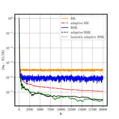
For each experiment, we run independent trials each starting with the initial iterate x0=0subscript𝑥00x_{0}=0 with the following parameters m=2000,n=100,σ=0.05,s=10formulae-sequence𝑚2000formulae-sequence𝑛100formulae-sequence𝜎0.05𝑠10m=2000,n=100,\sigma=0.05,s=10 and M=200𝑀200M=200, i.e. each block is of size mi=10subscript𝑚𝑖10m_{i}=10. The best parameter γ𝛾\gamma for every method aRSK and aRK were obtained by grid search over the set γ{0.005,0.01,0.05,0.1,1,2}𝛾0.0050.010.050.112\gamma\in\{0.005,0.01,0.05,0.1,1,2\}. We measured performance by plotting the average relative residual error 𝐀xkb2/b2subscriptnorm𝐀subscript𝑥𝑘𝑏2subscriptnorm𝑏2\|\mathbf{A}x_{k}-b\|_{2}/\|b\|_{2} and the relative error xkx^2/x^2subscriptnormsubscript𝑥𝑘^𝑥2subscriptnorm^𝑥2\|x_{k}-\hat{x}\|_{2}/\|\hat{x}\|_{2} against the number of iterations in Figure 2.

The RK and RSK methods will be our baseline comparisons. We did a small grid search and selected the λ𝜆\lambda that gives the smallest relative error for RSK and aRSK. With λ𝜆\lambda fixed for both RSK and aRSK, We used the same procedure to select γ𝛾\gamma for the aRSK and aRK(λ=0𝜆0\lambda=0). Having obtained the parameter for RSK, we can estimate γ𝛾\gamma and β0subscript𝛽0\beta_{0} with which we run haRSK.

Figure 2 shows in a semilog plot of the relative residuals and the relative reconstruction errors for all methods. Note that the usual RK and RSK methods reduce the error exponentially at the beginning and stagnate when the order of the total noise level is reached as predicted by Eq (4.1), whereas aRK, aRSK and haRSK thanks to their adaptive stepsize are able to bring down the residuals and the errors to zero according to Corollary 3.3. The parameters of aRK and aRSK giving the best results are obtained through a small grid search. After choosing λ𝜆\lambda and γ𝛾\gamma for aRK and aRSK we used the same λ𝜆\lambda for the haRSK method and estimated γ𝛾\gamma and β0subscript𝛽0\beta_{0} without knowing the true solution. In Figure 2 we see that haRSK has a better performance than the other adaptive methods. The reason behind this can be due to the fact that the best parameters were not part of the grid search space.

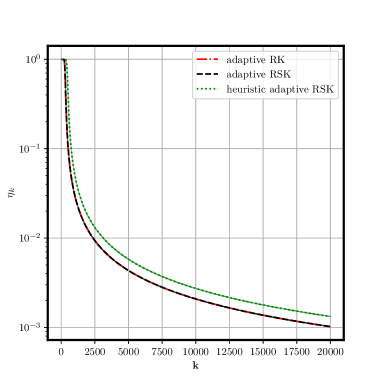
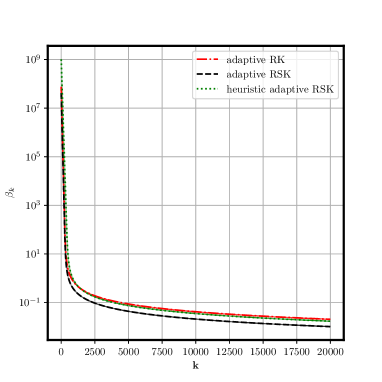
Figure 3 shows in a semilog plot how the parameters ηksubscript𝜂𝑘\eta_{k} and βksubscript𝛽𝑘\beta_{k} evolve during the iteration for all the adaptive methods. The stepsize for the haRSK has a slow decay compared to other stepsizes. All the stepsizes are starting near 1 and decreasing towards zero. The second plot shows the behavior of βksubscript𝛽𝑘\beta_{k} that governs the reconstruction error for different adaptive methods.

Refer to caption
Refer to caption
Figure 2: A comparison of the five methods as described in Section 5.1 for m=2000,n=100,formulae-sequence𝑚2000𝑛100m=2000,n=100, sparsity s=10𝑠10s=10, γaRK=0.05,γaRSK=0.1formulae-sequencesubscript𝛾𝑎𝑅𝐾0.05subscript𝛾𝑎𝑅𝑆𝐾0.1\gamma_{aRK}=0.05,\gamma_{aRSK}=0.1, λ=0.05𝜆0.05\lambda=0.05, N0=400,N1=100formulae-sequencesubscript𝑁0400subscript𝑁1100N_{0}=400,N_{1}=100. From our heuristics we obtained γ~=0.0777~𝛾0.0777\tilde{\gamma}=0.0777 and β~0=1022.60106subscript~𝛽01022.60superscript106\tilde{\beta}_{0}=1022.60*10^{6}. Left: Relative residual. Right: Relative error.
Refer to caption
Refer to caption
Figure 3: Evaluation of the stepsize ηksubscript𝜂𝑘\eta_{k} (left) and the parameter βksubscript𝛽𝑘\beta_{k} (right) in the runs of the adaptive methods in Figure 2.

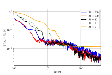
In another experiment, we investigated the influence of the number of blocks on convergence and recovery guarantee. We generated an m×n𝑚𝑛m\times n matrix with m=200𝑚200m=200 rows and n=100𝑛100n=100 columns and a vector x^n^𝑥superscript𝑛\hat{x}\in\mathbb{R}^{n} with s=10𝑠10s=10 non-zero entries. The right-hand side b𝑏b was always evaluated with independent noise with total noise level σ𝜎\sigma such that the relative error was 10%percent1010\%. We investigated numbers of blocks M{200,100,20,5,1}𝑀2001002051M\in\left\{200,100,20,5,1\right\}, each with equally sized blocks, i.e. block sizes of 1,2,10,40,2001210402001,2,10,40,200. We chose λ=1𝜆1\lambda=1. The hyperparameters β0subscript𝛽0\beta_{0} and γ𝛾\gamma depend on block size, and for a fair comparison we decided to use “best possible parameters”, i.e. we always used the exact value of β0subscript𝛽0\beta_{0} (using knowledge of ground truth x^^𝑥\hat{x}) and determined the best γ𝛾\gamma for each M𝑀M by a small grid search. The results are shown in Figure 4 in a log-log plot. One sees that the residual and error go down well below the noise level and also decay further but very slowly in the end. Both error and residual go down fast in the beginning and do so faster for a larger number of blocks, i.e. for smaller blocks. This phenomenon could be observed for other settings as well but depends on an accurate choice of the parameter γ𝛾\gamma.

Refer to caption
Refer to caption
Figure 4: The effect of the block number M𝑀M on the relative error versus epochs for Algorithm 1 (in the aRSK version) m=200,n=100,formulae-sequence𝑚200𝑛100m=200,n=100, sparsity s=10𝑠10s=10, γ𝛾\gamma determined by grid search, β0subscript𝛽0\beta_{0} exact. Left: Relative residual. Right: Relative error.

5.2 Computerized tomography

As an example on computerized tomography (CT), we used the implementation of the Radon transform from the Python library skimage and use it to build a system matrix for a parallel beam CT for a phantom of size N×N𝑁𝑁N\times N with N=50𝑁50N=50 and with 606060 equispaced angles. Hence, the system matrix 𝐀𝐀\mathbf{A} has size 3000×2500300025003000\times 2500, i.e. m=3000𝑚3000m=3000 and n=2500𝑛2500n=2500. We interpret the projection for each angle as one block 𝐀(i)subscript𝐀𝑖\mathbf{A}_{(i)}, i.e. we have M=60𝑀60M=60 and each block has the size mi=50subscript𝑚𝑖50m_{i}=50. The ground truth solution x^^𝑥\hat{x} is fairly sparse (see below) and we generated the exact right-hand side simply as b=𝐀x𝑏𝐀𝑥b=\mathbf{A}x. We used the total noise level of 10%percent1010\%, i.e. we choose σ=0.1b𝜎0.1delimited-∥∥𝑏\sigma=0.1\lVert b\rVert and σi=σ/Msubscript𝜎𝑖𝜎𝑀\sigma_{i}=\sigma/\sqrt{M}.

We used different methods for reconstruction, each run for 202020 epochs, i.e. for 60.00060.00060.000 iterations and using the function f(x)=λx1+12x22𝑓𝑥𝜆subscriptdelimited-∥∥𝑥112superscriptsubscriptdelimited-∥∥𝑥22f(x)=\lambda\lVert x\rVert_{1}+\tfrac{1}{2}\lVert x\rVert_{2}^{2}:

  1. 1.

    adaptive RSK: The adaptive randomized sparse Kaczmarz method, i.e. Algorithm 1 with stepsize ηksubscript𝜂𝑘\eta_{k} defined by (3.10), λ=30𝜆30\lambda=30, an educated guess for γ𝛾\gamma and exact value for β0subscript𝛽0\beta_{0} (using the knowledge of the ground truth solution).

  2. 2.

    RSK: The randomized sparse Kaczmarz method, i.e. Algorithm 1 with ηk=1subscript𝜂𝑘1\eta_{k}=1 (hence, neither γ𝛾\gamma nor β0subscript𝛽0\beta_{0} is needed, especially no ground truth knowledge is needed) and λ=30𝜆30\lambda=30.

  3. 3.

    heuristic adaptive RSK: the heuristic adaptive randomized sparse Kaczmarz method, i.e. Algorithm 1 with ηksubscript𝜂𝑘\eta_{k} from (3.10) and λ=30𝜆30\lambda=30. The parameters γ𝛾\gamma and β0subscript𝛽0\beta_{0} we estimated from the run of RSK as described in Section 4. We used N0=10.000subscript𝑁010.000N_{0}=10.000 in the estimate (4.2) of γ𝛾\gamma and N1=50.000subscript𝑁150.000N_{1}=50.000 in the estimate (4.3) for β0subscript𝛽0\beta_{0}.

  4. 4.

    adaptive RK: The adaptive randomized Kaczmarz method, i.e. Algorithm 1 with ηksubscript𝜂𝑘\eta_{k} defined by (3.10), λ=0𝜆0\lambda=0, an educated guess for γ𝛾\gamma and exact value for β0subscript𝛽0\beta_{0} (using the knowledge of the ground truth solution).

In other words: The RSK method would be our baseline comparison. It can be applied by just choosing λ𝜆\lambda by trial and error to adapt the sparsity of the outcome. With this, we can estimate the hyperparameter γ𝛾\gamma and β0subscript𝛽0\beta_{0} with which we run haRSK. This should produce a reconstruction which is much closer to the ground truth than RSK and even converge to the ground truth if the parameters were estimated exactly. The aRK and the aRSK method are just for further comparison.

To show the relevance of the ”independent noise” assumption, we conduct an additional experiment. Since the assumption of independent noise needs new measurements each time an equation is used, one could also try to do multiple measurements of the right hand side in advance and average the results to get improved measurement with lower noise and then reconstruct the solution. This is exactly what we do.

  1. 5.

    RSK avg: We sampled 20 noisy copies of b𝑏b with the same noise characteristic as other methods, we averaged those 20 copies into one vector bavgsubscript𝑏avgb_{\text{avg}} and ran the standard RSK method with bavgsubscript𝑏avgb_{\text{avg}} and ηk=1subscript𝜂𝑘1\eta_{k}=1 (hence, neither γ𝛾\gamma nor β0subscript𝛽0\beta_{0} is needed). We used λ=30𝜆30\lambda=30 as in the other methods.

In Figure 5 we show the ground truth data and the reconstructions by the adaptive RK, RSK, adaptive RSK and heuristic adaptive RSK. As can be seen, the sparse Kaczmarz methods all produce a clear background due to the sparsity enforcing f𝑓f. The adaptive RSK and the heuristic adaptive RSK also lead to less noise in the non-zero regions. In order to evaluate the quality of the reconstructed image in Figure 5 ensuring that optimization processes result in outputs that are perceptually similar or close to the original data, SSIM and PSNR two commonly used metrics are reported in Table 1.
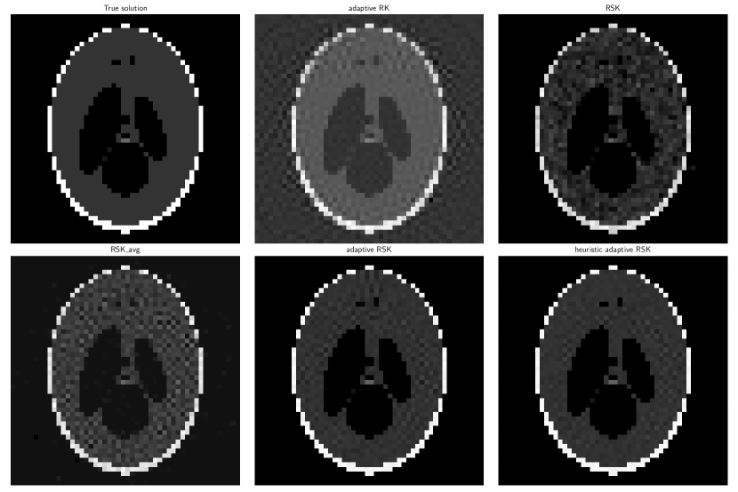
Refer to caption
Figure 5: Ground truth solution and reconstruction by the different methods.
Methods ARK RSK RSK avg ARSK hARSK
SSIM 0.884 0.925 0.918 0.990 0.993
PSNR 27.302 28.240 28.119 38.97 40.407
Table 1: Comparison of the SSIM and PSNR in Figure 5 for different methods: adaptive RK (ARK), RSK, RSK avg, adaptive RSK (ARSK) and heuristic adaptive RSK (hARSK).

SSIM [35] is used to measure how well the reconstructed output preserves the structural information of the original input. SSIM values range from -1 to 1. A value of 1 indicates a perfect similarity, while a value of -1 indicates complete dissimilarity. PSNR is used to quantify the quality of the reconstructed image by comparing it to the original image. Higher PSNR values indicate better quality. As we can see from Table 1, our two methods ARSK and hARSK are the ones giving the best reconstruction of our CT problem.

Figure 6 shows the relative residuals and the relative reconstruction errors for all methods. Averaging 20 noisy copies of b𝑏b reduce the variance by a factor of 2020\sqrt{20}. It can be observed that RSKavgsubscriptRSKavg\text{RSK}_{\text{avg}} is able to decrease faster at the beginning due to low noise variance but both residual and the reconstruction quality settle for worse values than using the adaptive stepsize. While the RSK method brings the residual down to some value in the order of the total noise level, the adaptive methods are able to go way below that and it seems that they even go down further. This indicates that the choice of parameters is quite accurate. We stress that the heuristic adaptive RSK does not need any knowledge of the true solution. The only choice that the user has to make is λ𝜆\lambda (to control the sparsity), and N0subscript𝑁0N_{0} and N1subscript𝑁1N_{1} for the estimation of γ𝛾\gamma and β0subscript𝛽0\beta_{0}. We also see that the reconstruction error for adaptive RSK and heuristic adaptive RSK keeps decaying until the last epoch (and is expected to go down even further). We find it quite remarkable that this is possible even though the heuristic adaptive RSK method only sees corrupted data (with independent noise). As expected, the error in RSK and adaptive RK stagnates at some level (RSK because it is not adaptive and adaptive RK because it does not respect the sparsity). Table 2 shows CPU times for different methods necessary to run for 20 epochs or to bring the relative error below a tolerance of 0.0780.0780.078 for Figure 6. We notice that ARSK and hARSK are the fattest methods to reach the tol meanwhile ARK and RSK are not able to reach the tolerance even after the total number of epochs.
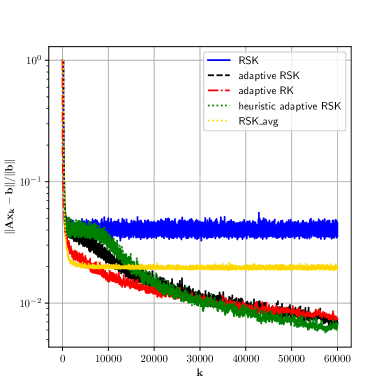
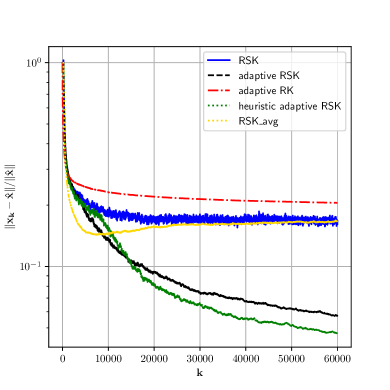
Refer to caption
Refer to caption
Figure 6: Left: Relative residuals for the CT reconstruction for the different methods. Right: Relative errors for the CT reconstruction.
CPU time (s)
ARK 192.456
RSK 264.749
RSK avg 215.851
ARSK 62.329
hARSK 58.539
Table 2: CPU time until a relative error falls below tol=0.078 for Figure 6. Here """""*" indicates that the relative error was not achieved after the total number of iterations.

We remark that the choice of N0subscript𝑁0N_{0} and N1subscript𝑁1N_{1} is crucial for a good estimate of the hyperparameters. The hyperparameter γ𝛾\gamma is related to the asymptotic exponential decay of the Bregman distance. This parameter is quite difficult to estimate since the RSK method converges and reduces the Bregman distance to the solution much faster in the first iterations than in the asymptotic regime. On the other hand, the asymptotic regime is cluttered with effects from the noise. We observed that a fairly large N0subscript𝑁0N_{0} lead to good results in most experiments. For the β0subscript𝛽0\beta_{0} used an even larger number, i.e. we used N1subscript𝑁1N_{1} large but only so large that the pre-asymptotic convergence has already happened.

6 Conclusion

In this work, we have proposed the block Bregman Kaczmarz using adaptive stepsize for solving finite dimensional linear inverse problems under the assumption of independent noise. In this setting, one never sees the noise-free right-hand side but always a new noisy version with noise being independent of every previous information and identically distributed. We showed that with a well-chosen stepsize (3.10) we are able to converge to the exact solution if we have access to a sufficient number of equations with independent noise. We gave a general error bound in terms of total noise variance σ2superscript𝜎2\sigma^{2}, the block number M𝑀M and the constant θ(x^)𝜃^𝑥\theta(\hat{x}). The stepsize depends on two parameters: the signal-to-noise ratio Dfx0(x0,x^)/σ2superscriptsubscript𝐷𝑓superscriptsubscript𝑥0subscript𝑥0^𝑥superscript𝜎2D_{f}^{x_{0}^{*}}(x_{0},\hat{x})/\sigma^{2} and the rate parameter γ𝛾\gamma. However, we showed in Section 4 how to estimate these unknown parameters after having chosen N0,N1subscript𝑁0subscript𝑁1N_{0},N_{1} and demonstrated in various scenarios in experiments the effectiveness of these estimations. We have shown in the experiments part that using a block size of 2 can already speed up the convergence a lot but in general taking a bigger block size gives us faster convergence results. It would be interesting to investigate how the actual rate 𝒪(k1/2)𝒪superscript𝑘12\mathcal{O}(k^{-1/2}) to recover the exact solution can be accelerated.

The heuristic estimates of the hyperparameters γ𝛾\gamma and β0subscript𝛽0\beta_{0} depend on the choices of N0subscript𝑁0N_{0} and N1subscript𝑁1N_{1}, respectively. While these values play a big role, one can usually get good values for these values by inspecting the decay of the residual of a standard Bregman-Kaczmarz run, keeping in mind which regimes should be used for the estimation of the hyperparameters (steady linear decay for γ𝛾\gamma and stagnation for β0subscript𝛽0\beta_{0}).

In this paper, we assumed that the blocks are fixed for the full run of the algorithm. We think that the results can be extended to a framework where the blocks of rows are newly sampled in each iteration (cf. [23, 33]) and expect that similar results than in this paper can be derived.

References

  • [1] Zhong-Zhi Bai and Wen-Ting Wu. On greedy randomized Kaczmarz method for solving large sparse linear systems. SIAM Journal on Scientific Computing, 40(1):A592–A606, 2018.
  • [2] Kui Du, Wu-Tao Si, and Xiao-Hui Sun. Randomized extended average block Kaczmarz for solving least squares. SIAM Journal on Scientific Computing, 42(6):A3541–A3559, 2020.
  • [3] Yonina C Eldar and Deanna Needell. Acceleration of randomized Kaczmarz method via the Johnson-Lindenstrauss lemma. Numerical Algorithms, 58:163–177, 2011.
  • [4] Tommy Elfving, Per Christian Hansen, and Touraj Nikazad. Semi-convergence properties of Kaczmarz’s method. Inverse problems, 30(5):055007, 2014.
  • [5] Heinz Werner Engl, Martin Hanke, and Andreas Neubauer. Regularization of inverse problems, volume 375. Springer Science & Business Media, 1996.
  • [6] Richard Gordon, Robert Bender, and Gabor T Herman. Algebraic reconstruction techniques (art) for three-dimensional electron microscopy and x-ray photography. Journal of theoretical Biology, 29(3):471–481, 1970.
  • [7] Robert M. Gower, Denali Molitor, Jacob Moorman, and Deanna Needell. On adaptive sketch-and-project for solving linear systems. SIAM Journal on Matrix Analysis and Applications, 42(2):954–989, 2021.
  • [8] Robert M Gower and Peter Richtárik. Randomized iterative methods for linear systems. SIAM Journal on Matrix Analysis and Applications, 36(4):1660–1690, 2015.
  • [9] Jamie Haddock and Anna Ma. Greed works: An improved analysis of sampling Kaczmarz-Motzkin. SIAM Journal on Mathematics of Data Science, 3(1):342–368, 2021.
  • [10] Jamie Haddock, Deanna Needell, Elizaveta Rebrova, and William Swartworth. Quantile-based iterative methods for corrupted systems of linear equations. SIAM Journal on Matrix Analysis and Applications, 43(2):605–637, 2022.
  • [11] Markus Haltmeier, Antonio Leitao, and Otmar Scherzer. Kaczmarz methods for regularizing nonlinear ill-posed equations i: Convergence analysis. Inverse Problems and Imaging, 1(2):289, 2007.
  • [12] Yuling Jiao, Bangti Jin, and Xiliang Lu. Preasymptotic convergence of randomized Kaczmarz method. Inverse Problems, 33(12):125012, 2017.
  • [13] S. Kaczmarz. Angenäherte Auflösung von Systemen linearer Gleichungen. Bull. Internat. Acad. Polon. Sci. Lettres A, pages 355–357, 1937.
  • [14] Barbara Kaltenbacher, Andreas Neubauer, and Otmar Scherzer. Iterative regularization methods for nonlinear ill-posed problems, volume 6 of Radon Series on Computational and Applied Mathematics. Walter de Gruyter GmbH & Co. KG, Berlin, 2008.
  • [15] Ji Liu and Stephen Wright. An accelerated randomized Kaczmarz algorithm. Mathematics of Computation, 85(297):153–178, 2016.
  • [16] Dirk A Lorenz, Frank Schöpfer, and Stephan Wenger. The linearized Bregman method via split feasibility problems: analysis and generalizations. SIAM Journal on Imaging Sciences, 7(2):1237–1262, 2014.
  • [17] Dirk A Lorenz, Stephan Wenger, Frank Schöpfer, and Marcus Magnor. A sparse Kaczmarz solver and a linearized Bregman method for online compressed sensing. In 2014 IEEE international conference on image processing (ICIP), pages 1347–1351. IEEE, 2014.
  • [18] Shuai Lu and Peter Mathé. Stochastic gradient descent for linear inverse problems in Hilbert spaces. Mathematics of Computation, 91(336):1763–1788, 2022.
  • [19] Nicholas F Marshall and Oscar Mickelin. An optimal scheduled learning rate for a randomized Kaczmarz algorithm. SIAM Journal on Matrix Analysis and Applications, 44(1):312–330, 2023.
  • [20] Cun-Qiang Miao and Wen-Ting Wu. On greedy randomized average block Kaczmarz method for solving large linear systems. Journal of Computational and Applied Mathematics, 413:114372, 2022.
  • [21] Jacob D Moorman, Thomas K Tu, Denali Molitor, and Deanna Needell. Randomized Kaczmarz with averaging. BIT Numerical Mathematics, 61:337–359, 2021.
  • [22] Jennifer L. Mueller and Samuli Siltanen. Linear and nonlinear inverse problems with practical applications, volume 10 of Computational Science & Engineering. Society for Industrial and Applied Mathematics (SIAM), Philadelphia, PA, 2012.
  • [23] Ion Necoara. Faster randomized block Kaczmarz algorithms. SIAM Journal on Matrix Analysis and Applications, 40(4):1425–1452, 2019.
  • [24] Deanna Needell. Randomized Kaczmarz solver for noisy linear systems. BIT Numerical Mathematics, 50:395–403, 2010.
  • [25] Deanna Needell and Joel A Tropp. Paved with good intentions: analysis of a randomized block Kaczmarz method. Linear Algebra and its Applications, 441:199–221, 2014.
  • [26] Stefania Petra. Randomized sparse block Kaczmarz as randomized dual block-coordinate descent. Analele Stiintifice Ale Universitatii Ovidius Constanta-Seria Matematica, 23(3):129–149, 2015.
  • [27] R. Tyrrell Rockafellar. Convex analysis, volume No. 28 of Princeton Mathematical Series. Princeton University Press, Princeton, NJ, 1970.
  • [28] Frank Schöpfer and Dirk A Lorenz. Linear convergence of the randomized sparse Kaczmarz method. Mathematical Programming, 173(1):509–536, 2019.
  • [29] Frank Schöpfer, Dirk A Lorenz, Lionel Tondji, and Maximilian Winkler. Extended randomized Kaczmarz method for sparse least squares and impulsive noise problems. Lineare Algebra and Applications, 652:132–154, 2022.
  • [30] Stefan Steinerberger. A weighted randomized Kaczmarz method for solving linear systems. Mathematics of Computation, 90(332):2815–2826, 2021.
  • [31] Stefan Steinerberger. Quantile-based random Kaczmarz for corrupted linear systems of equations. Information and Inference: A Journal of the IMA, 12(1):448–465, 2023.
  • [32] Thomas Strohmer and Roman Vershynin. A randomized Kaczmarz algorithm with exponential convergence. Journal of Fourier Analysis and Applications, 15(2):262–278, 2009.
  • [33] Lionel Tondji and Dirk A Lorenz. Faster randomized block sparse Kaczmarz by averaging. Numerical Algorithms, pages 1–35, 2022.
  • [34] Lionel Tondji, Dirk A. Lorenz, and Ion Necoara. An accelerated randomized Bregman-Kaczmarz method for strongly convex linearly constraint optimization*. In 2023 European Control Conference (ECC), pages 1–6, 2023.
  • [35] Zhou Wang, Alan C Bovik, Hamid R Sheikh, and Eero P Simoncelli. Image quality assessment: from error visibility to structural similarity. IEEE transactions on image processing, 13(4):600–612, 2004.
  • [36] Lu Zhang, Hongxia Wang, and Hui Zhang. Quantile-based random sparse Kaczmarz for corrupted, noisy linear inverse systems. arXiv preprint arXiv:2206.07356, 2022.
  • [37] Anastasios Zouzias and Nikolaos M Freris. Randomized extended Kaczmarz for solving least squares. SIAM Journal on Matrix Analysis and Applications, 34(2):773–793, 2013.