Certified Robust Models with Slack Control and Large Lipschitz Constants

Abstract

Despite recent success, state-of-the-art learning-based models remain highly vulnerable to input changes such as adversarial examples. In order to obtain certifiable robustness against such perturbations, recent work considers Lipschitz-based regularizers or constraints while at the same time increasing prediction margin. Unfortunately, this comes at the cost of significantly decreased accuracy. In this paper, we propose a ours that addresses this issue and improves certified robustness by tackling two problems: Firstly, commonly used margin losses do not adjust the penalties to the shrinking output distribution; caused by minimizing the Lipschitz constant $K$. Secondly, and most importantly, we observe that minimization of $K$ can lead to overly smooth decision functions. This limits the model’s complexity and thus reduces accuracy. Our ours addresses these issues by explicitly calibrating the loss w.r.t. margin and Lipschitz constant, thereby establishing full control over slack and improving robustness certificates even with larger Lipschitz constants. On CIFAR-10, CIFAR-100 and Tiny-ImageNet, our models consistently outperform losses that leave the constant unattended. On CIFAR-100 and Tiny-ImageNet, ours improves upon state-of-the-art deterministic $L_{2}$ robust accuracies. In contrast to current trends, we unlock potential of much smaller models without $K$=$1$ constraints.

1 Introduction

Figure 1: Existing Lipschitz margin methods control the Lipschitz constant $K$ to be low, yet we observe decision functions becoming overly smooth when $K$ is too low (left) – impairing accuracy. Our ours loss provides slack control, which we show is inversely proportional to $K$ (see gradients on top). We can control $K$ to be high, avoid the smoothing and achieve improved clean and robust accuracies (right). Incorrect or not robust samples marked red.

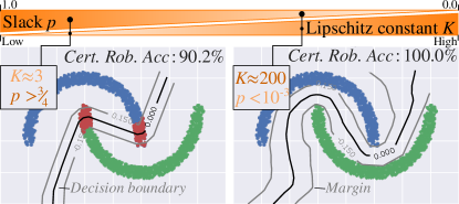
The Lipschitz constant $K$ of a classifier specifies the maximal change in output for a given input perturbation. This simple relation enables building models that are certifiably robust to constrained perturbations in the input space, i.e., those with $L_{2}$-norm below $\epsilon$. This is because the resulting output distance $K\cdot\epsilon$ can be calculated efficiently (i.e., in a closed form) without expensive test-time randomization, such as randomized smoothing [8], or network bound relaxations, e.g. [14, 50]. This way of obtaining certifiable robustness is also directly linked to large margin classifiers, as illustrated in figure 1, where a training sample free area of radius $\epsilon$ is created around the decision boundary. The earliest practical examples implementing Lipschitz margins for certified robustness include [16], which provided first guarantees on deep networks or LMT [38] and GloRo [25] that design Lipschitz margin losses.

A limitation with Lipschitz margin classifiers is their decreased performance, as has been shown on standard datasets like CIFAR-10 or TinyImageNet, both in terms of empirical robustness and clean accuracy. This is emphasized in particular when comparing to approaches such as adversarial training [28, 5] and its variants [49, 6, 45]. Thus, recent work proposed specialized architectures [7, 27, 1, 32, 29, 46, 37, 47, 30, 2, 42] to enforce specific Lipschitz constraints, adjusted losses [38, 25, 32, 47, 48, 30] or tighter upper Lipschitz bounds [24, 18, 10] to address these shortcomings. Despite existing efforts, clean and robust accuracy still lags behind state-of-the-art empirical results.

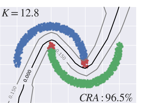
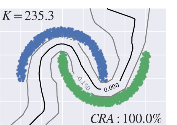
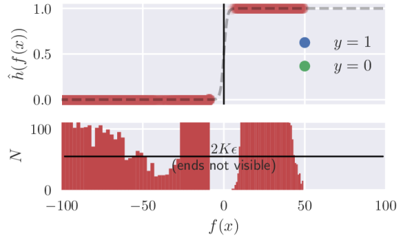
We relate this shortcoming to two interlinked properties of used losses: Firstly, logistic based margin losses, including GloRo [25], SOC [32] and CPL [29] do not adjust their output penalties to the output scaling caused by minimization of $K$. In practice, this results in samples remaining in under-saturated regions of the loss and effectively within margins. And secondly, we identify that controlling the Lipschitz constant $K$ to be too low, may result in overly smooth decision functions – impairing clean and robust accuracy. The result is exemplarily illustrated in figure 2(b) (middle) for GloRo on the two moons dataset. The induced overly smooth decision surface eventually leads to reduced clean and robust accuracy. Contributions: In this work, we propose ours, a loss with improved control over slack and Lipschitz constant $K$ to instrument models with a margin of width $2\epsilon$. Key to our loss is integrating the scale of the logistic loss with $K$, allowing calibration to the margin. This calibration endows ours with explicit control over slack and $K$, which can improve certified robust accuracy. As a result, the classifier avoids learning an overly smooth decision boundary while obtaining optimal margin, as illustrated for two moons in figure 2(c). On CIFAR-10, CIFAR-100 and Tiny-ImageNet, our method allows greater Lipschitz constants while at the same time having tighter bounds and yielding competitive certified robust accuracies (CRA). I.e. applying ours to existing training frameworks consistently improves CRA by multiple percentage points while maintaining or improving clean accuracy.

(a) Cross-Entropy

(b) GloRo

(c) Ours

Figure 2: We illustrate how our loss calibrates the logistic function of the loss w.r.t.  the margin, leading to improved clean and certified robust accuracy (CRA). (a) Cross-Entropy does not guarantee margins, the Lipschitz constant $K$ is large. (b) Uncalibrated margin losses such as GloRo may produce violated margins (gray) and decision boundaries (black) on the two-moons dataset. (c) In contrast, our calibrated loss is better visually and quantitatively for robust and accurate samples. The middle row plots their output probabilities.

2 Related Work

Lipschitz classifiers for robustness. For completeness, we note that many methods exist for certified robustness. For an extensive overview we refer the reader to a recent published summary [26]. Since their discovery in [36], many methods for certified robustness have been published [26]. Among others, Lipschitz regularization was considered as a potential way to improve robustness against adversarial examples. While such regularizers could only improve empirical robustness [7, 20, 17], local Lipschitz bounds where used to obtain certified robustness in [16] at the expense of additional calculations at inference. The use of global Lipschitz bounds has a key advantage over most other methods: certification at inference is deterministic and cheap to compute. Alas, it was originally considered intractable due to very loose bounds [16, 41]. More recently, however, a number of methods allow robustness certification based on global Lipschitz bounds, including [27, 1, 38, 32, 29, 30, 2, 42, 37, 25, 24, 18, 47, 48]. These improvements can fundamentally be attributed to two independent developments: (i) preventing gradient norm attenuation by specialized non-linearities to preserve classifier complexity [27, 1] and (ii) architectural constraints that guarantee a Lipschitz constant of $1$ [27, 37, 32, 29, 46, 30, 2, 42]. Additional work investigated the use of tighter bound estimation [41, 27, 13, 21, 18, 10]. Nevertheless, training deep Lipschitz networks with appropriate expressive power remains an open problem [19, 31]. We approach this issue using a novel loss that provides more control over the Lipschitz constant which bounds expressiveness [4].

Large margin for deep learning. Large margin methods have a long standing history in machine learning to improve generalization of learning algorithms, e.g., see  [39, 40, 9]. While margin optimization is actively researched in the context of deep learning, as well [35, 34, 33, 3, 12, 15], state-of-the-art deep networks usually focus on improving accuracy and remain vulnerable to adversarial examples [28, 5]. This indicates that the obtained margins are generally not sufficient for adversarial robustness. Moreover, the proposed margin losses often require expensive pairwise sample comparison [35], normalization of the spectral norm of weights [3] or linearization of the loss [12, 43, 11]. Adversarial training can also be viewed as large margin training [11], but does not provide certified robustness. This is the focus of our work.

3 ours

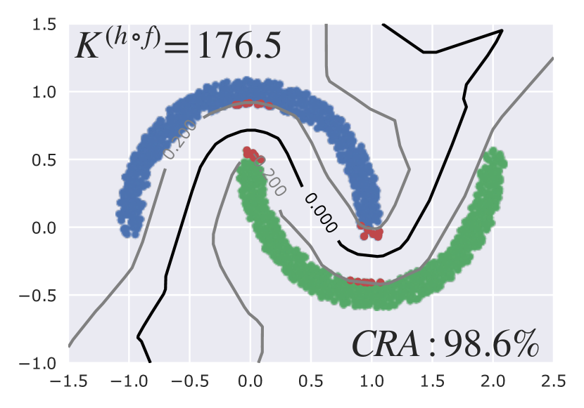
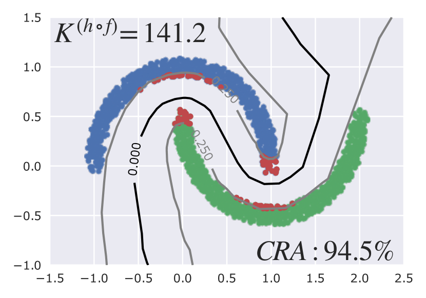
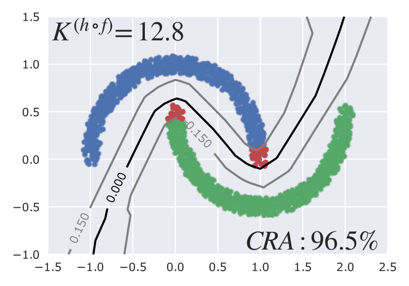
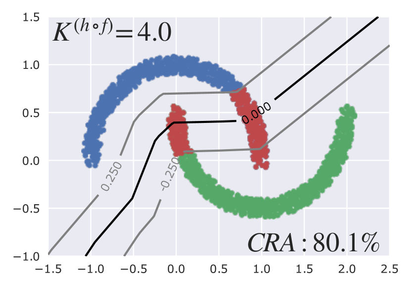
We propose a new margin loss called ours that calibrates the loss to the width of the margin – a property not explicitly accounted for in existing large margin Lipschitz methods. Specifically, we calibrate the logistic functions at the output (sigmoid and softmax), by integrating the Lipschitz constant $K$ into the definition of the logistic scale parameter. This new formulation reveals two properties important for margin training: (i) the scale parameter controls slackness and (ii) slackness influences classifier smoothness. This slack control allows to trade-off certified robust and clean accuracy. But more importantly, we find that this slackness determines $K$ of the whole model. This is illustrated on the two moons dataset in figure 1 (left) with high slack implying small $K$ and right with low slack implying large $K$. Given this improved control, we train models with large constants that produce new state-of-the-art robust accuracy scores.

3.1 Background

Let $(x,y)\in\mathcal{D_{X}}$ be a sample-label pair in a dataset in space $\mathcal{X}$, $f$ be a classifier $f:\mathcal{X}\to\mathcal{S}$ where $\mathcal{S}\subseteq\mathbb{R}^{N}$ is the logit space with $N$ logits and $h$ be a non-linearity like the logistic function or softmax mapping, e.g. $h:\mathcal{S}\to\mathbb{R}^{N}$.

Lipschitz continuity. The Lipschitz continuity states that for every function $f$ with bounded first derivative, there exists a Lipschitz constant $K$ that relates the distance between any two points $x_{1},x_{2}$ in input space $\mathcal{X}$ to a distance in output space. That is, for any input sample distance $\|x_{1}-x_{2}\|_{p}$, the resulting output distance $\|f(x_{1})-f(x_{2})\|_{p}$ is at most $K\cdot\|x_{1}-x_{2}\|_{p}$. Consequently, this inequality enables the construction of losses that measure distances in input space: e.g. the margin width – and importantly: quick input certification. E.g. assume a classifier with two logits $f_{1},f_{2}$. An input $x$ is certified robust w.r.t. radius $\epsilon$ when the Lipschitz bounded distance $\epsilon K$ is less than the distance between the two logits: $\epsilon K<|f_{1}(x)-f_{2}(x)|$. Note that $K$ is not required to be small to allow certification. The inequality also holds when $K$ is large, as long as the distance between logits is greater, as we will see in our experiments in section 4. The exact Lipschitz constant, though, is non-trivial to estimate for highly non-linear functions such as deep networks [41]. Fortunately, it is tractable to calculate an upper bound. For this, it is sufficient to be able to decompose the classifier $f$, e.g., a (convolutional) neural network, into its $L$ individual layers, i.e. $f=g^{(L)}\circ g^{(L-1)}\circ\dots\circ g^{(1)}$. Then $K$ is upper bounded by the product of norms [36],

$$K\leq\prod_{l=1}^{L}\|g^{(l)}\|_{p}=:\hat{K}.$$ (1)

In general, this bound is extremely loose without any form of Lipschitz regularization[41], yet recent work has shown substantially improved tightness, rendering uses in losses tractable (e.g. [25, 32, 29, 30, 2, 42, 18]).

Lipschitz Margin losses. To produce certified robust models, we strive to train models with large margins. This can be achieved by adapting the training objective and specifying a minimal distance $\epsilon$ between any training sample and the decision boundary. A typical example is the hinge loss formulation in SVMs [9]:

$$\min_{f}\mathbb{E}_{(x,y)\sim\mathcal{D_{X}}}\left[h\left(\epsilon-yf(x)\right)+\lambda\|f\|^{2}\right],$$ (2)

where $\epsilon=1$ and $h(\,\cdot\,)=\max\{\,\cdot\,,0\}$. $\|f\|$ denotes a generic measure of classifier complexity, which in the linear SVM case is the norm of the weight matrix. This formulation can be generalized to Lipschitz classifiers, e.g., by minimizing $\|f\|=K$ or by multiplying $\epsilon$ with its Lipschitz factor $\epsilon K$. The latter being used in the GloRo loss [25]. All variants of formulation (2) require strict minimization of $K$ to produce margins. We find these types of losses can be improved when $h$ belongs to the logistic family – as sigmoid and softmax are. Since logistic functions assume a fixed output distribution, we observe that minimizing $K$ can leave samples too close to the decision boundary We present exemplary evidence in figure 2(b) in which red samples remain within the margins. This is specifically true for GloRo, but also for methods that hard constrain $K$ (e.g. [32, 29, 46]). In the following, we address these issues with ours.

3.2 Binary ours

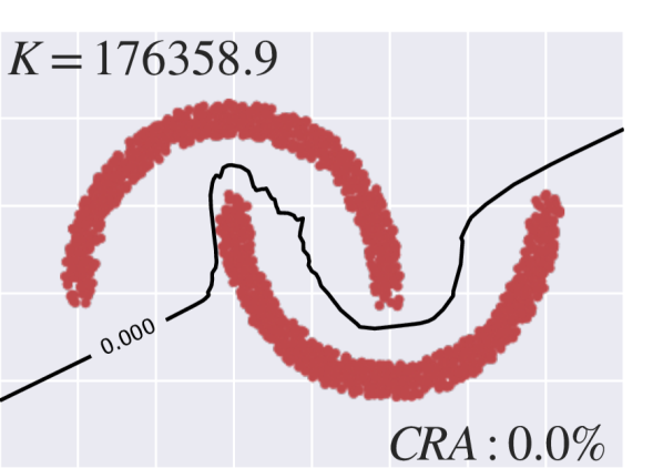
We base our construction of ours on the general margin formulation in equation (2). Key is calibrating the output non-linearity $h$ to the margin. In the binary case, it is common practice in deep learning to set $h$ in equation (2) to a logistic function $h(x)={[1+\exp\{-x/\sigma\}]^{-1}}$ with fixed $\sigma=1$ and minimize the binary cross-entropy loss. Yet the underlying logistic distribution assumes a fixed distribution width $\sigma=1$, which can be detrimental for training Lipschitz classifiers. To demonstrate the limitation of this assumption, we look at figure 2 illustrating margin training on the two-moons dataset. Figure 2(a) illustrates vanilla cross-entropy and no Lipschitz regularization. The decision boundary attains an irregular shape without margin. The Lipschitz constant is very high, the output values attain high probabilities since they are pushed to the tails of the distribution (see $p=h(f(x))$ in middle row). In contrast, a Lipschitz margin loss (GloRo [25], fig. 2(b)) produces a margin, yet non-robust samples (red) remain within margin boundaries. This is a consequence of minimizing $K$, which limits the spread of the distribution. Under this condition, the assumption $\sigma=1$ is inefficient. Additionally, since $\sigma$ of the logistic is fixed, the final probability $p$ at the margin $\pm\epsilon$ can only be determined post-hoc, after the Lipschitz constant $K$ finds a minimum. We can be more efficient about this process by calibrating the width to $K\epsilon$ at each training step and requiring $p$ at $\pm\epsilon$ to be a specific value. The result is shown in figure 2(c) which produces the desired margin with no errors. Our proposed loss is defined as follows.

Definition 1 - Binary ours. Let $y\in\{-1,1\}$, and $\mathcal{L}$ be the binary cross entropy loss $\mathcal{L}(y,h(f(x)))=-\log h(f(x))-(1-y)\log(1-h(f(x)))$. We propose the objective:

$$\min_{f} \,\,\mathbb{E}_{(x,y)\sim\mathcal{D_{X}}}\left[\mathcal{L}(y,\hat{h}(f(x);y))+\lambda K^{2}\right]$$ (3)

with $$\hat{h}(f(x);y)=h\left(-\frac{y\epsilon}{\sigma_{\epsilon}(p)}+\frac{1}{\sigma_{\epsilon}(p)}\frac{f(x)}{K}\right)$$ (4)

and $$\sigma_{\epsilon}(p)=\frac{2\epsilon}{h^{-1}(1-p)-h^{-1}(p)},$$ (5)

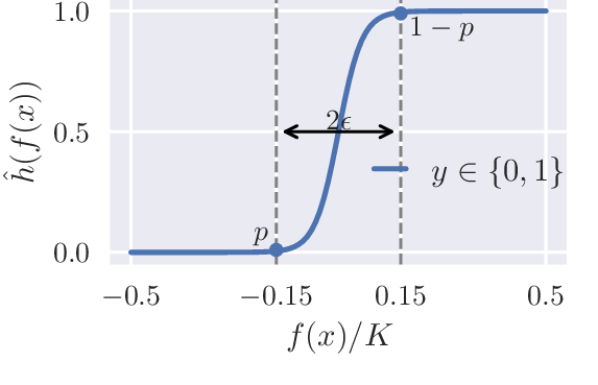
where $\hat{h}$ is our calibrated logistic and $h^{-1}$ is the inverse cdf: $h^{-1}(p)=\log(\nicefrac{{p}}{{1-p}})$. Our proposal follows from calibrating $\sigma$ to $2\epsilon$. For its realization we only require $4$ values to uniquely determine $\sigma$: (i) the two positions of the margin boundaries $\pm\epsilon$ and (ii) the two probabilities $p_{-\epsilon},p_{\epsilon}$ that the logistic distribution should attain at these positions. We illustrate these $4$ values in figure 3, which displays an already calibrated logistic function to $\epsilon=0.15$ (vertical lines) and $p_{-\epsilon}=p=10^{-3}$ and $p_{\epsilon}=1-p=1-10^{-3}$. The theoretical derivation follows from the logistic distribution, which we discuss in the supplement sec. A. We denote the calibrated scale as $\sigma_{\epsilon}(p)$ as it depends on $\epsilon$ and a probability $p$ (equation (5)). So far, this does not express the integration of the Lipschitz constant $K$. Recall that the input distance $2\epsilon$ can be related to the corresponding output distance via $K$, i.e. $2K\epsilon$. We consequently acquire the Lipschitz calibrated version shown in figure 3: $\nicefrac{{f(x)}}{{\sigma_{\epsilon}(p)K}}$. Next, we integrate hard margin offsets $\pm\epsilon$ as in formulation (2) to maximize the penalty on samples within the margin. To integrate, we add $\pm\epsilon K$, depending on the class sign: $[-yK\epsilon+f(x)]/[\sigma_{\epsilon}(p)K]$. This places the probability on the margin to the worst case value $0.5$. Note that this does not invalidate our calibration: the offset is a tool to improve margin training and is removed during inference. ours is easy to generalize to multinomial classification utilizing softmax. We show its implementation in the supplement, sec. A.

Figure 3: Calibrated logistic function as key to our ours loss by parameterizing the scale parameter $\sigma$ to margin width $2\epsilon$. Left: without margin offset; middle: with margin offset $\epsilon$; right: slack in ours is governed by parameter $p$. That is to increase slack, we increase $p$ which decreases loss for samples on the wrong margin side (indicated by arrows).

3.3 Discussion

ours is derived from joining the definition of $\sigma$ with the Lipschitz inequality while adjusting for the margin distance $2\epsilon$. By utilizing the Lipschitz constant, this scale parameter can be calibrated to the margin width as if measured in input space. This is feasible because of the normalization by the Lipschitz constant $\nicefrac{{f(x)}}{{K}}$ in equations (4). This normalization has two additional ramifications. First, it decouples the classifier constant from the loss. $K$ can attain any value, while ours ensures calibration. And secondly, the Lipschitz constant of the whole model $h(f(x))$ is solely dependent on $\sigma_{\epsilon}(p)$. That is $K^{\scalebox{0.5}{$(h\circ f)$}}=K^{\scalebox{0.5}{$(h)$}}=\nicefrac{{1}}{{\sigma_{\epsilon}(p)}}$. Below, we discuss the implications of ours with respect to the tightness of Lipschitz bounds, the interpretation of $\sigma$ as allowed slack and the classifier’s complexity.

Tightness. Tightness dictates the utility of the used Lipschitz bound. To measure, we can estimate a naïve lower bound to $K$ by finding the pair of training samples $x_{1},x_{2}$ that maximizes the quotient $\nicefrac{{\|f(x_{1})-f(x_{2})\|}}{{\|x_{1}-x_{2}\|}}$. Since the input sample distances remain fixed, tightness can only be increased by increasing output distances and bounding $K$ – conceptually bringing the two quantities closer together. Recall that typical losses assume a fixed output distribution $\sigma=1$. The capacity to push values into the saturated area of the loss is thereby limited. Tightness is thereby mainly achieved by minimizing $K$ because output distances cannot be increased significantly. ours instead, does not minimize $K$ but bounds it via normalization. Since our loss is calibrated to $K\epsilon$, we can achieve increased tightness by only maximizing output distances. With the difference of increasing output distances much farther than possible with other margin losses (an example is illustrated in figure 2 (compare x-axis of (b) and (c)). We find this to converge faster (see figure D1 in supplement) and achieve better robust accuracies than related work, as we present in section 4. However, since increasing output distances has a growth influence on $K$, we find it necessary to put slight regularization pressure on $K$ via factor $\lambda$, as stated on the RHS of equation (3).

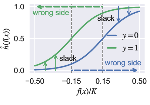
Slack. Since the logistic function has a smooth output transition from $0$ to $1$, values on the wrong margin side can be interpreted as slackness. We illustrate slack in figure 3 which shows a calibrated logistic as in figure 3 and indicates wrong margin sides for each class by dashed arrows. Consider class $y=1$ in green. If a sample falls on the wrong margin side (anywhere along the green arrow at the top) the probability decreases and consequently the loss increases (i.e., negative log-likelihood $\lim_{p\to 0}-\log(p)=\infty$). The governing factor for slack in our loss is the probability $p$ in $\sigma_{\epsilon}(p)$ of equation 4, indicated by the green vertical arrows, which implicitly defines the loss magnitude for samples on the wrong margin side. Note that without calibration, we find the logistic $\sigma$ or temperature in softmax to have no slack effect. We provide empirical evidence in the supplement, sec. D.

Classifier complexity. [4] derive complexity bounds for a $2$-layered neural network (theorem 18). I.e., given $2$ layers with weight norm $B$ and $1$ and non-linearity with Lipschitz constant $L$, the Gaussian complexity of the model is bounded by their product $K=B\cdot L\cdot 1$. This directly applies to hard-constrained $K$=$1$ models, but we find it applies to soft-constrained models as well. Effectively, this bound has implications for training Lipschitz classifiers: if $K$ is too small, it restricts the models ability to fit the data. While theory provides only an upper bound, we find empirical evidence as support. That is, clean and certified robust accuracy can be improved when $L$ of the loss is adjusted – and thus $K$. We find strongest evidence on two-moons (figure 4, bottom row), and consistent support on image data (section 4). With decreasing $K$ (top), the model becomes overly smooth, losing performance. ours offers direct control over $K$, simply by adjusting slack. That is, $K$ is inversely proportional to the slack $p$: $K^{\scalebox{0.5}{$(h\circ f)$}}=\nicefrac{{1}}{{\sigma_{\epsilon}(p)}}$. Consequently, for a fixed $\epsilon$, slack bounds the complexity of the model. Models that can separate the data well require little slack, implying a larger $K^{\scalebox{0.5}{$(h\circ f)$}}$. The next section discusses this in more detail.

Ours

(a) $2\epsilon=0.2$

(b) $2\epsilon=0.3$
(True margin)

(c) $2\epsilon=0.4$

(d) $2\epsilon=0.5$

GloRo

Figure 4: Our ours (top row) vs margin loss GloRo (bottom) on two-moons. Red points denote incorrect or non-robust samples. GloRos formulation leads to consistently smaller Lipschitz constant $K^{\scalebox{0.5}{$(h\circ f)$}}$ restricting the classifier complexity. Already for the true margin $2\epsilon=0.3$ it fits inefficiently. For “too-large” margins, GloRo eventually degenerates to a failure case with a near linear decision boundary. In contrast, our ours produces a $100\%$ accurate and robust model for the true margin and retains sensible margins for increased $\epsilon$.

4 Evaluation

ours offers increased control over slack and classifier complexity, discussed in section 3.3. In this section, we present empirical evidence for these claims. We show that decreasing slack leads to models with less smooth decision boundaries, resulting in higher clean and certified robustness. To this end, we present results on the synthetic two-moons dataset by visualizing the produced margins and discuss the application on natural images: CIFAR-10, CIFAR-100 [22] and Tiny-ImageNet [23]. Implementation of our method involves computing the upper Lipschitz bound. We measure the width of the margin with the $L_{2}$ distance. Consequently, we implement equation (1) with the product of spectral norms [36] and calculate them by performing power iterations. Our training strategy follows the respective method we compare with. That is, we reuse published code (where available) but use our loss. To evaluate, we measure certified robust accuracies (CRA) for three margin widths ($36/255$, $72/255$, $108/255$) and Lipschitz bound tightness. CRA represents the average number of accurately classified samples that are also robust (fall outside the margin). The latter is the fraction between empirical lower bound and upper bound. All training and metric details are listed in the supplement, sec. B and C. Our code is made publicly available at github.com/mlosch/CLL.

4.1 Two-moons dataset

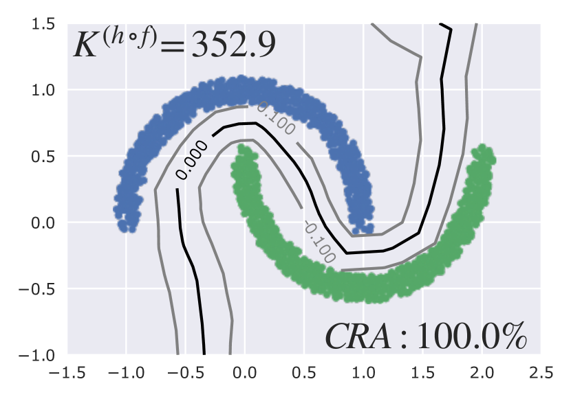
We start with an analysis on two-moons in order to visualize learned decision boundaries and investigate the connection to the Lipschitz constant. using uniform sampled noise of radius $0.1$ around each sample. This results in a true-margin of exactly $2\epsilon=0.3$. In figure 4, we exemplarily compare ours with GloRo, training 7-layered networks for different target margin widths (columns). Individual plots display the decision boundary (black line) and the Lipschitz margin (gray lines). CRAs and Lipschitz constants $K^{\scalebox{0.5}{$(h\circ f)$}}$ are reported in the corners, non-robust or misclassified training samples are marked red. GloRo already loses CRA at the true margin $2\epsilon$ and the decision boundary becomes very smooth with decreasing $K^{\scalebox{0.5}{$(h\circ f)$}}$. In contrast, ours retains $100\%$ CRA for the true margin and only slowly loses CRA beyond. The key is in the control over slack and hence $K^{\scalebox{0.5}{$(h\circ f)$}}$ – we set $p=10^{-12}$ in equation 4. Our decision functions do not become overly smooth.

4.2 Image datasets

We continue our discussion on CIFAR-10, CIFAR-100 and Tiny-ImageNet, evaluating multiple architectures: On CIFAR-10/100, we evaluate 6C2F[24], 4C3F[44], LipConv[32] and XL[29, 2]. On Tiny-ImageNet, we consider 8C2F[24], LipConv, XL and LBDN[42]. We report Tiny-ImageNet results in table 1 and CIFAR results in table 2, considering CRA for three different margin widths and clean accuracy. Hereby, all values produced with ours are averages over $9$ runs with different random seeds. Standard deviations are reported in the supplement, sec D. Additionally, we report tightness and Lipschitz constants of both the classifier $f$, as well as the composition with the loss $h\circ f$ – stating the effective complexity of the model. $\overline{K}^{\scalebox{0.5}{$(f)$}}$ and $\overline{K}^{\scalebox{0.5}{$(h\circ f)$}}$ state the largest constant between pairs of classes, e.g. $\overline{K}^{\scalebox{0.5}{$(f)$}}=\max_{i,j}\hat{K}^{\scalebox{0.5}{$(f)$}}_{i,j}$. Hereby, data scaling factors (e.g. normalization) influence $K^{\scalebox{0.5}{$(h\circ f)$}}$. E.g. a normalization factor of $5$, increases $K^{\scalebox{0.5}{$(h\circ f)$}}$ by the same factor.

Table 1: Results on Tiny-ImageNet on clean and certified robust accuracy (CRA) for six different methods using Lipschitz bounds $\overline{K}^{\scalebox{0.5}{$(h\circ f)$}}$. Applying ours to existing methods consistently improves certified robust accuracy (CRA). Architectures evaluated: 8C2F[24], LipConv[32], XL[29, 2] and Sandwich[42] $\top$ indicates model is additionally trained with TRADES-loss[49]. $\dagger$-flagged numbers are reproduced values with our own code. ours numbers are averaged over $9$ runs.

		Method	Model	Clean (%)	CRA $\frac{36}{255}$ (%)	CRA $\frac{72}{255}$ (%)	CRA $\frac{108}{255}$(%)	$\overline{K}^{\scalebox{0.5}{$(f)$}}$	$\overline{K}^{\scalebox{0.5}{$(h\circ f)$}}$	Tightness (%)
Tiny-ImageNet		GloRo[25]	8C2F⊤	35.5	22.4	-	-	12.5		47
			8C2F${}^{\top}\dagger$	39.5	23.9	14.3	9.0	3.9		53
		Local-Lip-B[18]	8C2F	36.9	23.4	12.7	6.1	-	-	-
		Ours $\epsilon=0.5,p=0.01$	8C2F	39.8 (+0.3)	25.9 (+2.0)	16.5 (+2.2)	10.7 (+1.7)	288.3	10.6	64 (+11)
		SOC[32]	LipConv-10	32.1	21.5	12.4	7.5	6.4		85
			LipConv-20	31.7	21.0	12.9	7.5	6.4		81
		Ours	LipConv-20	32.6 (+0.5)	26.0 (+3.5)	20.2 (+7.3)	15.5 (+8.0)	4.9	11.6	84 (+3)
		SLL[2]	XL	32.1	23.2	16.8	12.0	-	-	-
		LBDN[42]	Sandwich	33.4	24.7	18.1	13.4	-	-	-
		Ours $\epsilon=1.0,p=0.025$	8C2F	33.5 (+0.1)	25.3 (+0.6)	19.0 (+0.9)	13.8 (+0.4)	24.4	4.4	73

Table 2: Continuation of table 1 but on CIFAR-10 and CIFAR-100. Additional architectures evaluated: 4C3F[44], 6C2F[24]. Local-Lip-B tightness is estimated by reading values off of figure 2a [18].

		Method	Model	Clean (%)	CRA $\frac{36}{255}$ (%)	CRA $\frac{72}{255}$ (%)	CRA $\frac{108}{255}$(%)	$\overline{K}^{\scalebox{0.5}{$(f)$}}$	$\overline{K}^{\scalebox{0.5}{$(h\circ f)$}}$	Tightness (%)
CIFAR-10		Local-Lip-B[18]	6C2F	77.4	60.7	-	-	7.5		$\approx$80
		GloRo[25]	6C2F	77.0	58.4	-	-	15.8		70
			4C3F$\dagger$	77.4	59.6	40.8	24.8	7.4		71
		Ours	6C2F	77.6 (+0.6)	61.3 (+2.9)	43.5	27.7	709.3	11.6	78 (+8)
			4C3F	77.6 (+0.2)	61.4 (+1.8)	44.2 (+3.4)	29.1 (+4.3)	72.1	11.6	80 (+9)
		SOC[32]	LipConv-20	76.3	62.6	48.7	36.0	5.6		86
		Ours	LipConv-20	77.4 (+1.1)	64.2 (+1.6)	49.5 (+0.8)	36.7 (+0.7)	35.8	14.7	86
		CPL[29]	XL	78.5	64.4	48.0	33.0	$\sqrt{2}$		78
		Ours	XL	78.8 (+0.3)	65.9 (+1.5)	51.6 (+3.6)	38.1 (+5.1)	34.6	11.8	80 (+2)
		SLL[2]	XL	73.3	65.8	58.4	51.3	$\sqrt{2}$	6.7	88
		Ours	XL	73.0	65.5	57.8	51.0	59.4	10.6	88.0
CIFAR-100		SOC[32]	LipConv-20	47.8	34.8	23.7	15.8	6.5		85 (+1)
		Ours	LipConv-20	48.2 (+0.4)	35.1 (+0.3)	25.3 (+1.6)	18.3 (+2.5)	45.4	9.2	84
		CPL[29]	XL	47.8	33.4	20.9	12.6	1.6		74
		Ours	XL	47.9 (+0.1)	36.3 (+2.9)	28.1 (+7.2)	21.5 (+8.9)	42.0	7.6	79 (+5)
		SLL[2]	XL	46.5	36.5	29.0	23.3	1.5	6.0	81
		Ours	XL	46.9 (+0.4)	36.6 (+0.1)	29.0	23.4 (+0.1)	1.3	6.5	80

Certified robust accuracy. For fair comparison, we adjust $\epsilon$ and $p$ of ours to match or outperform clean accuracy of the respective baseline (details in supplement, sec. D). First, we consider Tiny-ImageNet (table 1). 8C2F is used to compare GloRo, Local-Lip-B and ours, LipConv is used to compare SOC and ours and SLL on XL and LBDN on Sandwich is compared to ours on 8C2F. Here, GloRo on 8C2F achieves $23.9\%$ CRA for $\epsilon=36/255$ and $39.5\%$ clean accuracy. Trained with ours, we achieve a substantial increase for the same margin of $25.9\%(+2.0)$ while improving clean accuracy $39.8\%(+0.3\%)$. We note that GloRo additionally uses the TRADES-loss [49] on 8C2F to trade-off clean for robust accuracy. ours simplifies this trade-off control via slack parameter $p$, see section 4.3. Regarding SOC on LipConv, we find $10$ layers to perform slightly better than $20$ (training setup in supplement, sec B). This is in line with the observation in [32]: adding more layers can lead to degrading performance. ours, in contrast, clearly outperforms SOC on $20$ layers with $26.0\%(+3.5)$ CRA ($\epsilon=36/255$), $15.5\%(+8.0)$ CRA ($\epsilon=108/255$) and $32.6\%(+0.5)$ clean accuracy on LipConv-20. These CRAs outperform the recent best methods SLL and LBDN. Differently to the AOL loss used in SLL and LBDN ours also enables soft-constrained architectures like 8C2F to achieve sota-performances. I.e., when choosing a lower slack value $p=0.025$ and $\epsilon_{\textit{train}}=1.0$, ours on 8C2F out-competes even LBDN [42]. I.e., we increase CRAs for $\epsilon=36/255$ to $25.3\%(+0.6)$ and for $\epsilon=108/255$ to $13.8\%(+0.4)$ while maintaining clean accuracy $33.5\%(+0.1)$. Interestingly, 8C2F has fewer parameters than Sandwich and XL: $4.3M$ vs $39M$ vs $1.1B$ [42],

Next, we consider CIFAR-10 and CIFAR-100 (table 2) GloRo applied to 6C2F and 4C3F produces a CRA ($\epsilon=36/255$) of under $60\%$ ($58.4\%$ and $59.6\%$ respectively) on CIFAR-10. Note that our reimplementation of GloRo improves CRA to $59.6\%(+1.2)$ upon the reported baseline in [25]. Replaced with ours, we report gains to $61.3\%(+2.9)$ and $61.4\%(+1.8)$ respectively. Additionally, we increase clean accuracy to $77.6\%$ for both ($+0.6$ and $+0.2$ respectively). Thereby, outperforming the local Lipschitz bound extension Local-Lip-B[18] ($60.7\%$ CRA), which utilizes expensive sample dependent local Lipschitz bounds to increase tightness. We also compare to SOC [32], CPL [29] and SLL [2], which constrain all layers to have Lipschitz constant $1$. Here, we consider the LipConv-20 architecture for SOC and the XL-architectures for CPL and SLL. LipConv-20 contains $20$ layers and XL $85$. SOC achieves a clean accuracy of $76.3\%$ on CIFAR-10, which ours improves to $77.4\%(+1.1)$ while also improving CRA on all tested margins. E.g. for $\epsilon=36/255$ we report a gain to $64.2\%(+1.6)$ and for $\epsilon=128/255$ a gain to $36.7\%(+0.7)$. Similarly, when applying ours to CPL-XL, we report CRA gains to $65.9\%(+1.5)$ and $38.1\%(+5.1)$ ($\epsilon=36/255$ and $\epsilon=128/255$ respectively) while retaining clean accuracy ($+0.3$). However, ours on SLL-XL provides no improvements. This is due to SLL using the AOL-loss [30], which has similar properties to ours on $K$=$1$ constrained models. We provide a discussion in the supplement, sec. D. On CIFAR-100 though, ours provides improvements on all tested models. On CPL-XL, we improve CRA on $\epsilon=108/255$ to $21.5\%(+8.9)$ while retaining clean accuracy $47.9\%(+0.1)$. On SLL, we report slight gains in clean accuracy to $46.9\%(+0.4)$ and CRA ($+0.1$ for both $\epsilon=36/255$ and $\epsilon=128/255$).

$\epsilon_{\text{train}}$ GloRo Ours 0.15 58.8 60.6 (+3.0$\%$) 0.25 49.6 51.6 (+4.0$\%$) 0.50 35.9 37.0 (+3.0$\%$) 0.75 27.0 28.7 (+6.3$\%$) 1.00 21.2 22.5 (+6.3$\%$) 1.25 16.9 17.4 (+3.3$\%$)

Figure 5: Left column: Slack governs robust accuracy trade-off in 4C3F on CIFAR-10. Remaining columns: Under increasing $0.15\leq\epsilon\leq 1.25$ on CIFAR-10, we compare our method with GloRo on 4C3F. We report consistently better CRA with at least $3\%$ improvement (left table). Our Lipschitz bounds are less constrained and $K^{\scalebox{0.5}{$(f)$}}$ is decoupled from the loss (middle figure). And lastly, our method produces tighter bounds (right).

Lipschitz bound and tightness. ours offers increased control over the Lipschitz bound of the model $K^{\scalebox{0.5}{$(h\circ f)$}}$. Across all datasets, we find ours to increase the Lipschitz constant $K^{\scalebox{0.5}{$(h\circ f)$}}$ over the respective baselines (while improving clean and robust accuracies). On soft-constrained models like 8C2F on Tiny-ImageNet, ours allows a doubling of the constant over GloRo ($7.3$ vs $3.9$). Similarly, on the hard-constrained model LipConv-20 on Tiny-Imagenet, we observe another doubling over SOC ($11.6$ vs $6.4$). This is consistent with $K^{\scalebox{0.5}{$(h\circ f)$}}$ on CIFAR. $K^{\scalebox{0.5}{$(h\circ f)$}}$ of LipConv-20 is increased with ours from $5.6$ to $14.7$. We note an exception for methods that utilize the AOL-loss [30]: SLL and LBDN. On these models, we find the constant $K^{\scalebox{0.5}{$(h\circ f)$}}$ to be highly similar, e.g. SLL-XL on CIFAR-100 ($K^{\scalebox{0.5}{$(h\circ f)$}}=6$ vs $6.5$). Importantly, these constant changes come with increased tightness as well. On Tiny-ImageNet, we increase tightness from $53\%$ to $64\%(+11)$ on 8C2F over GloRo and from $81\%$ to $84\%(+3)$ on LipConv-20 over SOC. Similarly, on CIFAR-10, we increase tightness from $71\%$ to $80\%$ on 4C3F over GloRo. In general, we observe the largest tightness improvements on soft-constrained models, although improvements on CPL are substantial. Here we gain, $+2$ and $+5$ percent points on CIFAR-10 and CIFAR-100 respectively.

4.3 Analysis and ablation

We considered different design choices when training with ours. An important aspect being the robust accuracy trade-off, which we investigate in the following by controlling slack. Furthermore, we investigate the bound, tightness and CRA over increasing margin width on CIFAR-10. An extended discussion on selecting $\epsilon$ and $p$ is discussed on 8C2F for Tiny-ImageNet in the supplement, sec D.

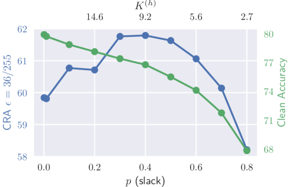
Slack. As discussed in section 3.3, we can regard the calibration probability $p$ as slack, which trades-off CRA and clean accuracy. We report both on 4C3F for $p\in[0.01,0.8]$ in figure 5 (left). An increase in $p$ decreases clean accuracy (green) from $80\%$ to $68\%$ but CRA increases to a peak at $p=0.4$ with $61.9\%$.

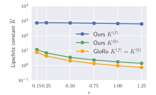
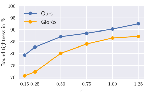
Increasing margin width. In addition to our main results, we compare ours and GloRo for larger $\epsilon$. We train all experiments on 4C3F. Different from before, we evaluate not for $\epsilon=\nicefrac{{36}}{{255}}$ but for the trained target, such that $\epsilon_{\text{train}}=\epsilon_{\text{test}}$. The table in figure 5, reports CRA and relative improvement over GloRo. With a minimum of $3\%$, we report consistent relative improvement for all $\epsilon$. The two right most plots of figure 5, display the Lipschitz constants across $\epsilon$ and tightness respectively. We see ours utilizing higher $K^{\scalebox{0.5}{$(h\circ f)$}}$ throughout while maintaining higher tightness. Note that $K^{\scalebox{0.5}{$(f)$}}$ remains fairly unconstrained at $\approx 10^{3}$ with ours, which is regularized via parameter $\lambda$. We analyzed its effect by choosing values from $10^{-15}$ to $10^{-1}$ and present results in figure D4a in the supplement. We find the performance of the model to be insensitive within $\lambda\in[10^{-10},10^{-3}]$.

5 Conclusion

We proposed a new loss, ours, for Lipschitz margin training that is calibrated to the margin width. ours reveals two intriguing properties: (i) the calibrated distribution width can be interpreted as slackness and (ii) slackness governs the smoothness of the model – and thereby the Lipschitz constant. The ramifications are important for improving certified robustness with Lipschitz constants. The constant can be large – implying increased model complexity and accuracy – if the model is capable of separating the data well. We illustrated these mechanics on two-moons, highlighting the implications for Lipschitz margin training and provided additional results on CIFAR-10, CIFAR-100 and Tiny-ImageNet. Applied across a wide range of datasets and methods, ours consistently improved clean and certified robustness.

References

- [1] Anil, C., Lucas, J., Grosse, R.: Sorting out lipschitz function approximation. ICML (2019)
- [2] Araujo, A., Havens, A.J., Delattre, B., Allauzen, A., Hu, B.: A unified algebraic perspective on lipschitz neural networks. ICLR (2023)
- [3] Bartlett, P.L., Foster, D.J., Telgarsky, M.J.: Spectrally-normalized margin bounds for neural networks. NeurIPS (2017)
- [4] Bartlett, P.L., Mendelson, S.: Rademacher and gaussian complexities: Risk bounds and structural results. JMLR (2002)
- [5] Carlini, N., Athalye, A., Papernot, N., Brendel, W., Rauber, J., Tsipras, D., Goodfellow, I.J., Madry, A., Kurakin, A.: On evaluating adversarial robustness. ICLR (2019)
- [6] Carmon, Y., Raghunathan, A., Schmidt, L., Duchi, J.C., Liang, P.S.: Unlabeled data improves adversarial robustness. NeurIPS (2019)
- [7] Cisse, M., Bojanowski, P., Grave, E., Dauphin, Y., Usunier, N.: Parseval networks: Improving robustness to adversarial examples. ICML (2017)
- [8] Cohen, J., Rosenfeld, E., Kolter, Z.: Certified adversarial robustness via randomized smoothing. ICML (2019)
- [9] Cortes, C., Vapnik, V.: Support-vector networks. Machine learning (1995)
- [10] Delattre, B., Barthélemy, Q., Araujo, A., Allauzen, A.: Efficient bound of lipschitz constant for convolutional layers by gram iteration. ICML (2023)
- [11] Ding, G.W., Sharma, Y., Lui, K.Y.C., Huang, R.: Mma training: Direct input space margin maximization through adversarial training. ICLR (2019)
- [12] Elsayed, G., Krishnan, D., Mobahi, H., Regan, K., Bengio, S.: Large margin deep networks for classification. NeurIPS (2018)
- [13] Fazlyab, M., Robey, A., Hassani, H., Morari, M., Pappas, G.: Efficient and accurate estimation of lipschitz constants for deep neural networks. NeurIPS (2019)
- [14] Gowal, S., Dvijotham, K.D., Stanforth, R., Bunel, R., Qin, C., Uesato, J., Arandjelovic, R., Mann, T., Kohli, P.: Scalable verified training for provably robust image classification. ICCV (2019)
- [15] Guo, Y., Zhang, C.: Recent advances in large margin learning. PAMI (2021)
- [16] Hein, M., Andriushchenko, M.: Formal guarantees on the robustness of a classifier against adversarial manipulation. NeurIPS (2017)
- [17] Hoffman, J., Roberts, D.A., Yaida, S.: Robust learning with jacobian regularization. arXiv preprint (2019)
- [18] Huang, Y., Zhang, H., Shi, Y., Kolter, J.Z., Anandkumar, A.: Training certifiably robust neural networks with efficient local lipschitz bounds. NeurIPS (2021)
- [19] Huster, T., Chiang, C.Y.J., Chadha, R.: Limitations of the lipschitz constant as a defense against adversarial examples. ECML PKDD (2018)
- [20] Jakubovitz, D., Giryes, R.: Improving dnn robustness to adversarial attacks using jacobian regularization. ECCV (2018)
- [21] Jordan, M., Dimakis, A.G.: Exactly computing the local lipschitz constant of relu networks. NeurIPS (2020)
- [22] Krizhevsky, A., Hinton, G., et al.: Learning multiple layers of features from tiny images. Technical report (2009)
- [23] Le, Y., Yang, X.: Tiny imagenet visual recognition challenge. Technical report (2014)
- [24] Lee, S., Lee, J., Park, S.: Lipschitz-certifiable training with a tight outer bound. NeurIPS (2020)
- [25] Leino, K., Wang, Z., Fredrikson, M.: Globally-robust neural networks. ICML (2021)
- [26] Li, L., Xie, T., Li, B.: Sok: Certified robustness for deep neural networks. SP (2023)
- [27] Li, Q., Haque, S., Anil, C., Lucas, J., Grosse, R.B., Jacobsen, J.H.: Preventing gradient attenuation in lipschitz constrained convolutional networks. NeurIPS (2019)
- [28] Madry, A., Makelov, A., Schmidt, L., Tsipras, D., Vladu, A.: Towards deep learning models resistant to adversarial attacks. ICLR (2018)
- [29] Meunier, L., Delattre, B.J., Araujo, A., Allauzen, A.: A dynamical system perspective for lipschitz neural networks. ICML (2022)
- [30] Prach, B., Lampert, C.H.: Almost-orthogonal layers for efficient general-purpose lipschitz networks. ECCV (2022)
- [31] Rosca, M., Weber, T., Gretton, A., Mohamed, S.: A case for new neural networks smoothness constraints. ”I Can’t Believe It’s Not Better!”NeurIPS workshop (2020)
- [32] Singla, S., Singla, S., Feizi, S.: Improved deterministic l2 robustness on cifar-10 and cifar-100. ICLR (2021)
- [33] Sokolić, J., Giryes, R., Sapiro, G., Rodrigues, M.R.: Robust large margin deep neural networks. IEEE Transactions on Signal Processing (2017)
- [34] Sun, S., Chen, W., Wang, L., Liu, T.Y.: Large margin deep neural networks: Theory and algorithms. arXiv preprint (2015)
- [35] Sun, Y., Chen, Y., Wang, X., Tang, X.: Deep learning face representation by joint identification-verification. NeurIPS (2014)
- [36] Szegedy, C., Zaremba, W., Sutskever, I., Bruna, J., Erhan, D., Goodfellow, I., Fergus, R.: Intriguing properties of neural networks. ICLR (2014)
- [37] Trockman, A., Kolter, J.Z.: Orthogonalizing convolutional layers with the cayley transform. ICLR (2020)
- [38] Tsuzuku, Y., Sato, I., Sugiyama, M.: Lipschitz-margin training: Scalable certification of perturbation invariance for deep neural networks. NeurIPS (2018)
- [39] Vapnik, V.: Estimation of dependences based on empirical data. Springer Science & Business Media (1982)
- [40] Vapnik, V.N.: An overview of statistical learning theory. IEEE transactions on neural networks (1999)
- [41] Virmaux, A., Scaman, K.: Lipschitz regularity of deep neural networks: analysis and efficient estimation. NeurIPS (2018)
- [42] Wang, R., Manchester, I.: Direct parameterization of lipschitz-bounded deep networks. ICML (2023)
- [43] Wei, C., Ma, T.: Improved sample complexities for deep neural networks and robust classification via an all-layer margin. ICLR (2019)
- [44] Wong, E., Schmidt, F., Metzen, J.H., Kolter, J.Z.: Scaling provable adversarial defenses. NeurIPS (2018)
- [45] Wu, D., Xia, S.T., Wang, Y.: Adversarial weight perturbation helps robust generalization. NeurIPS (2020)
- [46] Xu, X., Li, L., Li, B.: Lot: Layer-wise orthogonal training on improving l2 certified robustness. NeurIPS (2022)
- [47] Zhang, B., Cai, T., Lu, Z., He, D., Wang, L.: Towards certifying l-infinity robustness using neural networks with l-inf-dist neurons. ICML (2021)
- [48] Zhang, B., Jiang, D., He, D., Wang, L.: Boosting the certified robustness of l-infinity distance nets. ICLR (2022)
- [49] Zhang, H., Yu, Y., Jiao, J., Xing, E., El Ghaoui, L., Jordan, M.: Theoretically principled trade-off between robustness and accuracy. ICML (2019)
- [50] Zhang, H., Chen, H., Xiao, C., Gowal, S., Stanforth, R., Li, B., Boning, D., Hsieh, C.J.: Towards stable and efficient training of verifiably robust neural networks. ICLR (2020)