Spatiotemporal Patterns Induced by Turing-Hopf Interaction and Symmetry on a Disk

Abstract

Turing bifurcation and Hopf bifurcation are two important kinds of transitions giving birth to inhomogeneous solutions, in spatial or temporal ways. On a disk, these two bifurcations may lead to equivariant Turing-Hopf bifurcations. In this paper, normal forms for three kinds of Turing-Hopf bifurcations are given and the breathing, standing wave-like, and rotating wave-like patterns are found in numerical examples.
 
Keywords: Turing-Hopf bifurcation, Disk, Breathing oscillation, Standing wave, Rotating wave

I Introduction

In many reaction-diffusion equations, complex Turing-Hopf spatiotemporal patterns may appear, which is usually used as an explanation for many dynamic phenomena in chemical reactions, epidemics, and metapopulation models (Camara et al., 2016; Yang and Song, 2016; Cao and Jiang, 2018; Kumari and Mohan, 2020; Kumar and Gangopadhyay, 2020). Mathematically, the solution of the reaction-diffusion equation is often written in the form of $u_{j}(\vec{x},t)=u_{j0}\mathrm{e}^{\mathrm{i}\vec{q}\cdot\vec{x}+\sigma t}$ (Cross and Hohenberg, 1993) to characterize its spatiotemporal dynamics, where $\vec{q}$ is the wave vector and $\sigma$ is the eigenvalue with the largest real part. For a Turing-Hopf bifurcation, $\vec{q}$ is nonzero and $\sigma$ is also an imaginary value $\mathrm{i}\omega$. Thus, there exists the interaction of two Fourier modes (Perraud et al., 1993; Heidemann et al., 1993; Vallette et al., 1994; Song and Zou, 2014; An and Jiang, 2018).

There are many methods for studying the Turing-Hopf bifurcation. In numerical experiments, simple hexagonal arrangements of spots, stripes, and other spatiotemporal patterns can be observed in chemical reactions, semiconductors, predator-prey models, and other systems through numerical tools, indicating that this bifurcation can reveal some complex spatiotemporal patterns of dynamic systems (Rovinsky and Menzinger, 1992; Meixner et al., 1997; Bose et al., 2000; Baurmann et al., 2007). In physics, researchers often use multi-scale methods to derive the amplitude equation of the Turing-Hopf bifurcation to analyze pattern formations (Just et al., 2001; Venkov et al., 2007; Ledesma-Durán and Aragón, 2020). Moreover, in recent years, scholars have begun to use normal forms to analyze Turing-Hopf bifurcation. In particular, Song et al. (Song et al., 2016) and Jiang et al. (Jiang et al., 2020) derived the normal form of the Turing-Hopf bifurcation of partial differential equations (PDEs) and partial functional differential equations (PFDEs), respectively. Following the method proposed, there are many subsequent works on normal forms of the Turing-Hopf bifurcation (Song et al., 2019; Wu and Zhao, 2020; Lv, 2021; Duan et al., 2022).

However, most of these previous works have focused on one-dimensional intervals, and a few of them considered two-dimensional spaces, for example, rectangular domains (Just et al., 2001; Cao and Jiang, 2018; Chen et al., 2021) and circular domains(Abid et al., 2015; Paquin-Lefebvre et al., 2019), in which more abundant spatiotemporal patterns will be generated. In fact, the complex spatiotemporal patterns appearing in circular domains can be studied through the equivariant bifurcation. Precisely, the works on symmetric group theory in (Golubitsky et al., 1989) and the theory of equivariant normal forms in (Guo and Wu, 2013) are required. Equivariant Turing-Hopf bifurcation with time delay on a disk has not been considered, to our best knowledge. Therefore, in this paper, we consider a delayed general reaction-diffusion system with homogeneous Neumann boundary conditions on a disk and aim to explain many interesting spatiotemporal patterns induced by Turing-Hopf interaction and the symmetry.

Compared to previous work, our research in this paper has several new features. We gave formulas of the equivariant normal forms truncated to the third order of a general reaction-diffusion system on a disk and divided them into three types: ET-H, T-EH, and ET-EH bifurcations, according to different structure of the center subspace of the equilibrium. We characterize the long-term asymptotic behavior of the solution by normal forms, which can explain the occurrence of many patterns in real life more fitly. The theoretical results indicate the existence of several kinds of interesting patterns, including breathing, standing wave-like, rotating wave-like patterns and so on.

The rest of the paper is organized as follows. In Section II, We give preliminaries required for normal form derivation, including the definition of phase space, the eigenvalue problem of the Laplace operator on a circular domain, and the necessary assumptions for bifurcation. In Section III, main results of normal forms for ET-H, T-EH, and ET-EH bifurcations on a disk are shown respectively. In Section IV, two delayed mussel-algae systems are selected. Rich spatiotemporal patterns are observed near the Turing-Hopf points.

II Preliminaries

We consider a general delayed reaction-diffusion system of $n$ equations with homogeneous Neumann boundary conditions defined on a disk as follows:

$$\frac{\partial U(t,r,\theta)}{\partial t}=D(\mu)\Delta_{r\theta}U(t,r,\theta)+L(\mu)U_{t}(r,\theta)+F\left(U_{t}(r,\theta),\mu\right),~{}(r,\theta)\in\mathbb{D},~{}t>0,$$ (1)

where $\Delta_{r\theta}U=\frac{\partial^{2}U}{\partial r^{2}}+\frac{1}{r}\cdot\frac{\partial U}{\partial r}+\frac{1}{r^{2}}\cdot\frac{\partial^{2}U}{\partial\theta^{2}},~{}\mathbb{D}=\{(r,\theta):0\leq r\leq R,0\leq\theta\leq 2\pi\},~{}{U}_{t}(\vartheta)(r,\theta)=U(t+\vartheta,r,\theta),~{}\vartheta\in[-1,0)$. Here, we normalize the maximum delay to 1. To study the interaction between Turing instability and Hopf bifurcation, we usually select two parameters, i.e. $\mu=(\mu_{1},\mu_{2})\in\mathbb{R}^{2}$.

When considering a reaction-diffusion equation with time delay, one usually use the phase space of functions (Hale, 1977; Wu, 1996),

$${\mathscr{C}}:=C([-1,0],{\mathscr{X}_{\mathbb{C}}}),$$

where ${\mathscr{X}_{\mathbb{C}}}$ is the complexification of

$${\mathscr{X}}=\left\{\tilde{u}(r,\theta)\in{W}^{2,2}(\mathbb{D}):\partial_{r}\tilde{u}(R,\theta)=0,~{}\theta\in[0,2\pi)\right\},$$

with $\mathbb{L}^{2}$ inner product $\langle u(r,\theta),v(r,\theta)\rangle=\iint_{\mathbb{D}}ru(r,\theta)\bar{v}(r,\theta)\mathrm{d}r\mathrm{d}\theta$ weighted $r$. ${U}_{t}\in\mathscr{C}^{n},~{}L:\mathbb{R}\times{\mathscr{C}^{n}}\rightarrow\mathscr{X}_{\mathbb{C}}^{n}$ is a bounded linear operator, and ${F}:{\mathscr{C}}^{n}\times\mathbb{R}\rightarrow\mathscr{X}_{\mathbb{C}}^{n}$ is $C^{k}~{}(k\geq 3)$. Here we only consider the zero equilibrium, that is to say, we assume $F(0,\mu)=0,~{}\forall\mu\in\mathbb{R}^{2}$.

For $\mu=(\mu_{1},\mu_{2})$, the Taylor expansions of $L(\mu)$ and ${D}(\mu)$ are

$$D(\mu)=D_{0}+\mu_{1}D_{1}^{(1,0)}+\mu_{2}D_{1}^{(0,1)}+\frac{1}{2}\left(\mu_{1}^{2}D_{2}^{(2,0)}+2\mu_{1}\mu_{2}D_{2}^{(1,1)}+\mu_{2}^{2}D_{2}^{(0,2)}\right)+\cdots,$$

and

$$L(\mu)=L_{0}+\mu_{1}L_{1}^{(1,0)}+\mu_{2}L_{1}^{(0,1)}+\frac{1}{2}\left(\mu_{1}^{2}L_{2}^{(2,0)}+2\mu_{1}\mu_{2}L_{2}^{(1,1)}+\mu_{2}^{2}L_{2}^{(0,2)}\right)+\cdots.$$

Separating the linear part from system (1) yields

$$\frac{\partial U(t)}{\partial t}=\tilde{L}U_{t}+\tilde{F}(U_{t},\mu),$$ (2)

where $\tilde{L}U=D_{0}\Delta_{r\theta}U+L_{0}U$ with $D_{0}=D(0),~{}L_{0}=L(0)$, and $\tilde{F}(U_{t},\mu)=[D(\mu)-D_{0}]\Delta_{r\theta}U+[L(\mu)-L_{0}]U_{t}+F(U_{t},\mu)$.

The characteristic equation of the linearized equation at zero solution of (2) is

$$\prod_{m_{1}}{\Gamma_{0m_{1}}(\gamma)}\prod_{n,m_{2}}{\tilde{\Gamma}_{nm_{2}}(\gamma)}=0,$$ (3)

with

$$\Gamma_{0m_{1}}(\gamma)=\mathrm{det}\left[\gamma I+\lambda_{0m_{1}}D_{0}-L_{0}(\mathrm{e}^{\gamma\cdot}I)\right]=0,~{}m_{1}=0,1,2,\cdots,$$ (4)

$$\tilde{\Gamma}_{nm_{2}}(\gamma)=\mathrm{det}\left[\gamma I+\lambda_{nm_{2}}D_{0}-L_{0}(\mathrm{e}^{\gamma\cdot}I)\right]^{2}=0,~{}n=1,2,\cdots,~{}m_{2}=1,2,\cdots,$$

and

$$\lambda_{nm}=\left\{\begin{array}[]{ll}\frac{\alpha_{0m_{1}}^{2}}{R^{2}},&m_{1}=0,1,2,\cdots,\\ \frac{\alpha_{nm_{2}}^{2}}{R^{2}},&n=1,2,\cdots,~{}m_{2}=1,2,\cdots,\end{array}\right.$$

where $-\alpha_{0m_{1}}$ and $-\alpha_{nm_{2}}$ are eigenvalues of the Laplacian on the unit disk, see (Murray, 2001; Pinchover and Rubinstein, 2005; Chen et al., 2023) and the corresponding unit eigenfuncitons of the Laplacian are

$$\hat{\phi}_{nm}^{\lambda}=\left\{\begin{array}[]{ll}\hat{\phi}_{0m_{1}}^{c},&m_{1}=0,1,2,\cdots,\\ \hat{\phi}_{nm_{2}}^{c},~{}\phi_{nm_{2}}^{s},&n=1,2,\cdots,~{}m_{2}=1,2,\cdots,\end{array}\right.$$

with

$$\hat{\phi}_{0m_{1}}^{c}=\frac{J_{0}\left(\frac{\alpha_{0m_{1}}}{R}r\right)}{\|J_{0}\left(\frac{\alpha_{0m_{1}}}{R}r\right)\|},~{}\hat{\phi}_{nm_{2}}^{c}=\frac{J_{n}\left(\frac{\alpha_{nm_{2}}}{R}r\right)\mathrm{e}^{\mathrm{i}n\theta}}{2\pi\|J_{n}\left(\frac{\alpha_{nm_{2}}}{R}r\right)\|},~{}\hat{\phi}_{nm_{2}}^{s}=\overline{\hat{\phi}_{nm_{2}}^{c}}=\frac{J_{n}\left(\frac{\alpha_{nm_{2}}}{R}r\right)\mathrm{e}^{-\mathrm{i}n\theta}}{2\pi\|J_{n}\left(\frac{\alpha_{nm_{2}}}{R}r\right)\|},$$

which form an orthonormal basis for $\mathscr{X}_{\mathbb{C}}$.

In order to consider the interaction of Turing instability and Hopf bifurcation, we list the following assumptions for $\mu=(0,0)$ in Table 1.

Table 1: Roots with zero real part of (3) and the dimension of the central subspace (dim).

	(ET-H)	(T-EH)	(ET-EH)
$\Gamma_{0m_{1}}$	$\pm\mathrm{i}\omega_{H_{1}}$	0
$\tilde{\Gamma}_{nm_{2}}$	0 (repeated)	$\pm\mathrm{i}\omega_{H_{2}}$ (repeated)	0 (repeated), $\pm\mathrm{i}\omega_{H_{3}}$ (repeated)
$m_{1},n,m_{2}$	$m_{1}=m_{H_{1}},n=n_{T_{1}},m_{2}=m_{T_{1}}$	$m_{1}=m_{T_{2}},n=n_{H_{2}},m_{2}=m_{H_{2}}$	$n=n_{T_{3}},m_{2}=m_{T_{3}},n=n_{H_{3}},m_{2}=m_{H_{3}}$
dim	4	5	6

• In (ET-EH), for example, the chosen indexes mean that $\tilde{\Gamma}_{n_{T_{3}}m_{T_{3}}}(0)=0,~{}\tilde{\Gamma}_{n_{H_{3}}m_{H_{3}}}(\pm\mathrm{i}\omega_{H_{3}})=0$.

Inspired by (Golubitsky et al., 1989; Guo and Wu, 2013), if (ET-H) holds, we call this is a ET-H bifurcation, which means, the center space is spanned by the eigenvectors of a repeated zero eigenvalue (both geometric multiplicity and algebraic multiplicity are two) and a pair of simple imaginary roots. Similarly, if (T-EH) holds, we call this a T-EH bifurcation. If (ET-EH) holds, we call this a ET-EH bifurcation.

III Main Results

In this section, based on the Turing-Hopf normal forms theory for reaction-diffusion systems in a one-dimensional interval (Song et al., 2016; Jiang et al., 2020), we will derive the normal forms for ET-H, T-EH, and ET-EH bifurcations on a disk, respectively. The normal forms for ET-H and T-EH bifurcations can be considered as parts of the normal form of the ET-EH bifurcation, and the derivation is somewhat simpler. Therefore, we first provide Theorem III.1 on normal forms for the ET-EH bifurcation ($n_{T_{3}}\neq 2n_{H_{3}}$) and Remark III.4 for $n_{T_{3}}=2n_{H_{3}}$, while the other two normal forms are presented as Corollaries III.5 and III.9. In addition, we provide approximate forms for the solutions restricted to the center subspace corresponding to several spatiotemporal patterns in Theorem III.2, Remarks III.6, III.8 and III.10.

III.1 ET-EH bifurcation

If (ET-EH) holds, the center subspace of the equilibrium is six-dimensional. After coordinate transformation, the normal form on the center manifolds can be transformed into a four-dimensional real ordinary differential equations (ODEs) with ${\rho}_{H^{1}},~{}{\rho}_{H^{2}},~{}{\rho}_{T^{1}}$ and ${\rho}_{T^{2}}$ as independent variables, where ${\rho}_{H^{i}},i=1,2$ are variables on the eigenspace corresponding to pure imaginary roots $\pm\mathrm{i}\omega_{H_{3}}$ (Hopf) and ${\rho}_{T^{i}},i=1,2$ correspond to the zero root (Turing). When $n_{T_{3}}\neq 2n_{H_{3}}$, the detailed derivation of the normal form is presented in Appendix A, and the specific transformation can be found in (25). When $n_{T_{3}}=2n_{H_{3}}$, there will be additional terms that make the normal form more complex. Therefore, we can obtain the following results.

Theorem III.1.

When $n_{T_{3}}\neq 2n_{H_{3}}$, the normal form truncated to the third order for the ET-EH bifurcation can be written in polar coordinates as

$$\dot{\rho}_{H^{1}}=(\epsilon_{1}(\mu)+c_{11}\rho_{H^{1}}^{2}+c_{12}\rho_{H^{2}}^{2}+c_{13}\rho_{T^{1}}\rho_{T^{2}})\rho_{H^{1}},$$ (5)

$$\dot{\rho}_{H^{2}}=(\epsilon_{1}(\mu)+c_{11}\rho_{H^{2}}^{2}+c_{12}\rho_{H^{1}}^{2}+c_{13}\rho_{T^{1}}\rho_{T^{2}})\rho_{H^{2}},$$

$$\dot{\rho}_{T^{1}}=(\epsilon_{2}(\mu)+c_{21}\rho_{H^{1}}^{2}+c_{22}\rho_{H^{2}}^{2}+c_{23}\rho_{T^{1}}\rho_{T^{2}})\rho_{T^{1}},$$

$$\dot{\rho}_{T^{2}}=(\epsilon_{2}(\mu)+c_{21}\rho_{H^{1}}^{2}+c_{22}\rho_{H^{2}}^{2}+c_{23}\rho_{T^{1}}\rho_{T^{2}})\rho_{T^{2}}.$$

Theorem III.2.

We are mainly concerned with the properties corresponding to the following fourteen equilibrium points of (5), which are separated into eight categories.
$($ET-EH-$\mathrm{i})$  $(\rho_{H^{1}},\rho_{H^{2}},\rho_{T^{1}},\rho_{T^{2}})=(0,0,0,0)$ corresponds to the origin in the six-dimensional phase space and stands for a stationary solution, which is spatially homogeneous.
$($ET-EH-$\mathrm{ii})$  $(\rho_{H^{1}},\rho_{H^{2}},\rho_{T^{1}},\rho_{T^{2}})=\left(0,0,\rho_{T^{1}},\rho_{T^{2}}\right)$ with $\rho_{T^{1}}\rho_{T^{2}}=-\epsilon_{2}(\mu)/c_{23}$, corresponds to a static Turing pattern.
$($ET-EH-$\mathrm{iii})$  $(\rho_{H^{1}},\rho_{H^{2}},\rho_{T^{1}},\rho_{T^{2}})=\left(0,\sqrt{\frac{-\epsilon_{1}(\mu)}{c_{11}}},0,0\right)$, for $\epsilon_{1}(\mu)c_{11}<0$, corresponds to a periodic solution in the subspace of $(z_{2},z_{3})$, which is a rotating wave solution. At this point, the periodic solution restricted to the center subspace has the following approximate form

$$U(t)(r,\theta)\approx\sum_{i=1}^{n}{2|p_{1i}|\sqrt{\frac{-\epsilon_{1}(\mu)}{c_{11}}}J_{n_{H_{3}}}(\sqrt{\lambda_{n_{H_{3}}m_{H_{3}}}}r)\cos(\mathrm{Arg}(p_{1i})+\omega_{H_{3}}t+n_{H_{3}}\theta)\mathbf{e}_{i}},$$

where $\mathbf{e}_{i}$ is the $i$th unit coordinate vector of $\mathbb{R}^{n}$ and $p_{1i},1\leq i\leq n$ are defined in Appendix A.
$($ET-EH-$\mathrm{iv})$  $(\rho_{H^{1}},\rho_{H^{2}},\rho_{T^{1}},\rho_{T^{2}})=\left(\sqrt{\frac{-\epsilon_{1}(\mu)}{c_{11}}},0,0,0\right)$, for $\epsilon_{1}(\mu)c_{11}<0$, corresponds to a a periodic solution in the subspace of $(z_{1},z_{4})$, which is rotating wave solution in the opposite direction as that in $\mathrm{(ii)}$. At this point, the periodic solution restricted to the center subspace has the following approximate form

$$U(t)(r,\theta)\approx\sum_{i=1}^{n}{2|p_{1i}|\sqrt{\frac{-\epsilon_{1}(\mu)}{c_{11}}}J_{n_{H_{3}}}(\sqrt{\lambda_{n_{H_{3}}m_{H_{3}}}}r)\cos(\mathrm{Arg}(p_{1i})+\omega_{H_{3}}t-n_{H_{3}}\theta){e}_{i}}.$$

$($ET-EH-$\mathrm{v})$  $(\rho_{H^{1}},\rho_{H^{2}},\rho_{T^{1}},\rho_{T^{2}})=\left(\sqrt{\frac{-\epsilon_{1}(\mu)}{c_{11}+c_{12}}},\sqrt{\frac{-\epsilon_{1}(\mu)}{c_{11}+c_{12}}},0,0\right)$ corresponds to a periodic solution, which is a standing wave. At this point, the periodic solution restricted to the center subspace has the following approximate form

$$U(t)(r,\theta)\approx\sum_{i=1}^{n}{4|p_{1i}|\sqrt{\frac{-\epsilon_{1}(\mu)}{c_{11}+c_{12}}}J_{n_{H_{3}}}(\sqrt{\lambda_{n_{H_{3}}m_{H_{3}}}}r)\cos(\mathrm{Arg}(p_{1i})+\omega_{H_{3}}t)\cos(n_{H_{3}}\theta){e}_{i}}.$$

$($ET-EH-$\mathrm{vi})$  $(\rho_{H^{1}},\rho_{H^{2}},\rho_{T^{1}},\rho_{T^{2}})=\left(0,\sqrt{\frac{c_{13}\epsilon_{2}(\mu)-c_{23}\epsilon_{1}(\mu)}{c_{23}c_{11}-c_{13}c_{22}}},\rho_{T^{1}},\rho_{T^{2}}\right)$ with $\rho_{T^{1}}\rho_{T^{2}}=-\frac{\epsilon_{1}(\mu)+c_{11}\rho_{H^{2}}^{2}}{c_{13}}$, or $\left(0,\sqrt{\frac{-\epsilon_{1}(\mu)}{c_{11}}},0,\rho_{T^{2}}\right)$ and $\left(0,\sqrt{\frac{-\epsilon_{1}(\mu)}{c_{11}}},\rho_{T^{1}},0\right)$ with $\frac{\epsilon_{1}(\mu)}{c_{11}}=\frac{\epsilon_{2}(\mu)}{c_{22}}$, correspond to three groups of ET-EH patterns. At these points, the solution of real form restricted to the center subspace has the following approximate form

$$U(t)(r,\theta)\approx \sum_{i=1}^{n}{2|p_{1i}|\rho_{H^{2}}J_{n_{H_{3}}}(\sqrt{\lambda_{n_{H_{3}}m_{H_{3}}}}r)\cos(\mathrm{Arg}(p_{1i})+\omega_{H_{3}}t+n_{H_{3}}\theta){e}_{i}}$$ (6)

$$+\xi_{T}\left(\rho_{T^{1}}+\rho_{T^{2}}\right)J_{n_{T_{3}}}(\sqrt{\lambda_{n_{T_{3}}m_{T_{3}}}}r)\cos(n_{T_{3}}\theta).$$

$($ET-EH-$\mathrm{vii})$  $(\rho_{H^{1}},\rho_{H^{2}},\rho_{T^{1}},\rho_{T^{2}})=\left(\sqrt{\frac{c_{13}\epsilon_{2}(\mu)-c_{23}\epsilon_{1}(\mu)}{c_{23}c_{11}-c_{13}c_{21}}},0,\rho_{T^{1}},\rho_{T^{2}}\right)$ with $\rho_{T^{1}}\rho_{T^{2}}=-\frac{\epsilon_{1}(\mu)+c_{11}\rho_{H^{1}}^{2}}{c_{13}}$, or $\left(\sqrt{\frac{-\epsilon_{1}(\mu)}{c_{11}}},0,0,\rho_{T^{2}}\right)$ and $\left(\sqrt{\frac{-\epsilon_{1}(\mu)}{c_{11}}},0,\rho_{T^{1}},0\right)$ with $\frac{\epsilon_{1}(\mu)}{c_{11}}=\frac{\epsilon_{2}(\mu)}{c_{22}}$, correspond to three groups of ET-EH patterns in the opposite direction as that in $\mathrm{(vi)}$. At these points, the solution restricted to the center subspace has the following approximate form

$$U(t)(r,\theta)\approx \sum_{i=1}^{n}{2|p_{1i}|\rho_{H^{1}}J_{n_{H_{3}}}(\sqrt{\lambda_{n_{H_{3}}m_{H_{3}}}}r)\cos(\mathrm{Arg}(p_{1i})+\omega_{H_{3}}t-n_{H_{3}}\theta){e}_{i}}$$ (7)

$$+\xi_{T}\left(\rho_{T^{1}}+\rho_{T^{2}}\right)J_{n_{T_{3}}}(\sqrt{\lambda_{n_{T_{3}}m_{T_{3}}}}r)\cos(n_{T_{3}}\theta).$$

$($ET-EH-$\mathrm{viii})$  $(\rho_{H^{1}},\rho_{H^{2}},\rho_{T^{1}},\rho_{T^{2}})=\left(\sqrt{\frac{c_{13}\epsilon_{2}(\mu)-c_{23}\epsilon_{1}(\mu)}{c_{23}(c_{11}+c_{12})-c_{13}(c_{21}+c_{22})}},\sqrt{\frac{c_{13}\epsilon_{2}(\mu)-c_{23}\epsilon_{1}(\mu)}{c_{23}(c_{11}+c_{12})-c_{13}(c_{21}+c_{22})}},\rho_{T^{1}},\rho_{T^{2}}\right)$ with $\rho_{T^{1}}\rho_{T^{2}}=-\frac{\epsilon_{1}(\mu)+(c_{11}+c_{12})\rho_{H^{1}}^{2}}{c_{13}}$, or $\left(\sqrt{\frac{-\epsilon_{1}(\mu)}{c_{11}+c_{12}}},\sqrt{\frac{-\epsilon_{1}(\mu)}{c_{11}+c_{12}}},\rho_{T^{1}},0\right)$ and $\left(\sqrt{\frac{-\epsilon_{1}(\mu)}{c_{11}+c_{12}}},\sqrt{\frac{-\epsilon_{1}(\mu)}{c_{11}+c_{12}}},0,\rho_{T^{2}}\right)$ with $\frac{\epsilon_{1}(\mu)}{c_{11}+c_{12}}=\frac{\epsilon_{2}(\mu)}{c_{21}+c_{22}}$ correspond to three groups of ET-EH patterns. At these point, the solution restricted to the center subspace has the following approximate form

$$U(t)(r,\theta)\approx \sum_{i=1}^{n}{4|p_{1i}|\rho_{H^{1}}J_{n_{H_{3}}}(\sqrt{\lambda_{n_{H_{3}}m_{H_{3}}}}r)\cos(\mathrm{Arg}(p_{1i})+\omega_{H_{3}}t)\cos(n_{H_{3}}\theta){e}_{i}}$$ (8)

$$+\xi_{T}\left(\rho_{T^{1}}+\rho_{T^{2}}\right)J_{n_{T_{3}}}(\sqrt{\lambda_{n_{T_{3}}m_{T_{3}}}}r)\cos(n_{T_{3}}\theta).$$

Remark III.3.

$($ET-EH-$\mathrm{vi})$-$($ET-EH-$\mathrm{viii})$ show three types of complex ET-EH patterns. We draw a schematic diagram in Figure 1 of the solution in $($ET-EH-$\mathrm{vi})$ with $n_{T_{3}}=1,m_{T_{3}}=1;~{}n_{H_{3}}=2,m_{H_{3}}=2$ and $\omega_{H_{3}}=1$ as an example, which is

$$U(t)(r,\theta)\approx J_{2}(\sqrt{\lambda_{22}}r)\cos(t+2\theta)+J_{1}(\sqrt{\lambda_{11}}r)\cos{\theta}.$$ (9)

The subfigures in the first row provide ET-EH patterns like (6) at $t=0,~{}T/3,~{}2T/3$, and $T$, respectively, where $T\approx 6$ is the period. Fixing $r=R$ and $r=R/2$, we find that despite (9) is a sum of two regular patterns generating from Hopf bifurcation and Turing instability, under the interaction of the two, the spatial form of (9) is quite complex, making it difficult to summarize general rule. Similarly, the solutions in (7) and (8) can be explained in the same way.

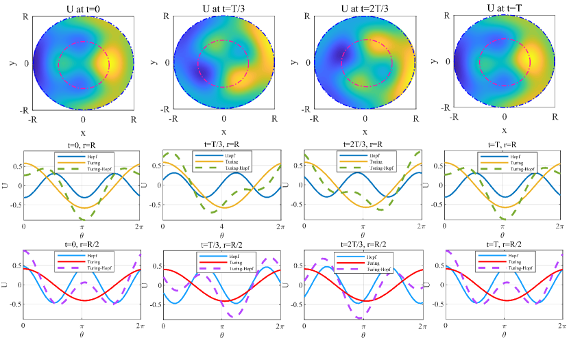
Figure 1: First row: ET-EH patterns in (9). Second/Third row: At $r=R/r=\frac{R}{2}$, the Hopf component, Turing component and there sum of (9) are illustrated.

Remark III.4.

When $n_{T_{3}}=2n_{H_{3}}$, there will be additional terms $B_{001010}z_{3}z_{5},~{}\overline{B_{001010}}z_{4}z_{5}$, $B_{001010}z_{1}z_{6}$, and $\overline{B_{001010}}z_{2}z_{6}$ in the normal form truncated to the third order for the ET-EH bifurcation. If we use the same coordinate transformation as that for $n_{T_{3}}\neq 2n_{H_{3}}$, there will be $\Delta\chi=\chi_{H^{1}}-\chi_{H^{2}}$ as a new variable, due to the presence of these additional terms. This means, by transformations $z_{1}=\rho_{H}\mathrm{e}^{\mathrm{i}\chi_{H^{1}}},~{}z_{4}=\rho_{H}\mathrm{e}^{-\mathrm{i}\chi_{H^{1}}},z_{3}=\rho_{H}\mathrm{e}^{\mathrm{i}\chi_{H^{2}}},~{}z_{2}=\rho_{H}\mathrm{e}^{-\mathrm{i}\chi_{H^{2}}},z_{5}=\rho_{T},~{}z_{6}=\rho_{T}$, we get the normal form written in polar coordinates as

$$\dot{\rho}_{H}=(\epsilon_{1}(\mu)+(c_{11}+c_{12})\rho_{H}^{2}+c_{13}\rho_{T}^{2}+c_{14}\rho_{T}\cos{\Delta\chi})\rho_{H},$$ (10)

$$\dot{\Delta\chi}=-2c_{14}\rho_{T}\sin{\Delta\chi},$$

$$\dot{\rho}_{T}=(\epsilon_{2}(\mu)+(c_{21}+c_{22})\rho_{H}^{2}+c_{23}\rho_{T}^{2})\rho_{T},$$

where $c_{14}=\mathrm{Re}\{B_{001010}\}$.

We are more concerned about the form of the original system solution corresponds to the equilibrium point of (10) with ${\rho}_{H}\neq 0,~{}{\rho}_{T}\neq 0$ and $\Delta\chi\neq 0$, for instance, $({\rho}_{H},{\rho}_{T},\Delta\chi)=\left(\sqrt{\frac{c_{23}\rho_{T}^{2}+\epsilon_{2}(\mu)}{c_{21}+c_{22}}},\right.$ $\left.\frac{-C_{2}\pm\sqrt{C_{2}^{2}-4C_{1}C_{3}}}{2C_{1}},\pi\right)$, with $C_{1}=(c_{11}+c_{12})c_{23}+(c_{21}+c_{22})c_{13},~{}C_{2}=\frac{-(c_{21}+c_{22})c_{14}\pi}{2}$, $C_{3}=(c_{11}+c_{12})\epsilon_{2}(\mu)+(c_{21}+c_{22})\epsilon_{1}(\mu)$. At these points, the solution restricted to the center subspace has the following approximate form

$$U(t)(r,\theta)\approx -\sum_{i=1}^{n}{4|p_{1i}|\rho_{H}J_{n_{H_{3}}}(\sqrt{\lambda_{n_{H_{3}}m_{H_{3}}}}r)\sin(\mathrm{Arg}(p_{1i})+\chi_{H^{1}}(t))\sin(n_{H_{3}}\theta){e}_{i}}$$ (11)

$$+2\xi_{T}\rho_{T}J_{n_{T_{3}}}(\sqrt{\lambda_{n_{T_{3}}m_{T_{3}}}}r)\cos(n_{T_{3}}\theta).$$

It can be observed that due to $\Delta\chi=\chi_{H^{1}}-\chi_{H^{2}}=\pi$, there is also a certain phase difference in the Hopf part and Turing part of the expression (11). Thus, the form of solution maintains standing wave characteristics (Hopf) and static pattern characteristics (Turing) at different positions on the disk.

III.2 ET-H bifurcation

If (ET-H) holds, compared to subsection III.1, the dimension of the eigenspace corresponding to pure imaginary roots $\pm\mathrm{i}\omega_{H_{2}}$ decreases. By (21) and (22), we can obtain the following results.

Corollary III.5.

The normal form truncated to the third order for ET-H bifurcation in polar coordinates is

$$\dot{\rho}_{H}=(\alpha_{1}(\mu)+a_{11}\rho_{H}^{2}+a_{12}\rho_{T^{1}}\rho_{T^{2}})\rho_{H},$$ (12)

$$\dot{\rho}_{T^{1}}=(\alpha_{2}(\mu)+a_{21}\rho_{T^{1}}\rho_{T^{2}}+a_{22}\rho_{H}^{2})\rho_{T^{1}},$$

$$\dot{\rho}_{T^{2}}=(\alpha_{2}(\mu)+a_{21}\rho_{T^{1}}\rho_{T^{2}}+a_{22}\rho_{H}^{2})\rho_{T^{2}}.$$

We can explain dynamics of the system by analyzing five equilibrium points of system (12). The equilibrium points $(0,0,0)$ and $(0,\rho_{T^{1}},\rho_{T^{2}})$ with $\rho_{T^{1}}\rho_{T^{2}}=-\frac{\alpha_{2}(\mu)}{a_{21}}$ are similar to $($ET-EH-$\mathrm{i})$-$($ET-EH-$\mathrm{ii})$, but the dynamic properties of the other equilibrium points are simpler than $($ET-EH-$\mathrm{vi})$-$($ET-EH-$\mathrm{viii})$. Therefore, we only provide the following remark.

Remark III.6.

$(\rho_{H},\rho_{T^{1}},\rho_{T^{2}})=\left(\sqrt{\frac{a_{12}\alpha_{2}(\mu)-a_{21}\alpha_{1}(\mu)}{a_{11}a_{21}-a_{12}a_{22}}},\rho_{T^{1}},\rho_{T^{2}}\right)$ with $\rho_{T^{1}}\rho_{T^{2}}=\frac{\alpha_{1}(\mu)+a_{11}\rho_{H}^{2}}{-a_{12}}$, or $(\sqrt{\frac{-\alpha_{1}(\mu)}{a_{11}}},\rho_{T^{1}},0)$ and $(\sqrt{\frac{-\alpha_{1}(\mu)}{a_{11}}},0,\rho_{T^{1}})$ with $\frac{\alpha_{1}(\mu)}{a_{11}}=\frac{\alpha_{2}(\mu)}{a_{22}}$, correspond to three groups of dynamic Turing-Hopf patterns (breathing patterns). At these points, the solution restricted to the center subspace has the following approximate form

$$U(t)(r,\theta)\approx \sum_{i=1}^{n}{2|p_{1i}|\rho_{H}J_{0}(\sqrt{\lambda_{0m_{T_{1}}}}r)\cos(\mathrm{Arg}(p_{1i})+\omega_{H_{1}}t){e}_{i}}$$

$$+\xi_{T}\left(\rho_{T^{1}}+\rho_{T^{2}}\right)J_{n_{T_{1}}}(\sqrt{\lambda_{n_{T_{1}}m_{T_{1}}}}r)\cos(n_{T_{1}}\theta).$$

Similar to the discussion in Remark III.3, the solution will maintain a fixed inhomogeneous form and oscillate up and down over time (breathing).

Remark III.7.

Let $\rho_{T}^{2}=\rho_{T^{1}}\rho_{T^{2}},~{}\bar{\rho}_{H}={\rho}_{H}\sqrt{|a_{11}|},~{}~{}\bar{\rho}_{T}={\rho}_{T}\sqrt{|a_{21}|}$, and drop the bars, then system (12) can be transformed into

$$\dot{\rho}_{H}=(\alpha_{1}(\mu)+\rho_{H}^{2}+a_{b}\rho_{T}^{2})\rho_{H},$$ (13)

$$\dot{\rho}_{T}=(\alpha_{2}(\mu)+a_{c}\rho_{H}^{2}+a_{d}\rho_{T}^{2})\rho_{T},$$

which has twelve distinct kinds of unfoldings. The stability conditions of equilibrium points can be given, by Chapter 7.5 in (Guckenheimer and Holmes, 1983). Thus, in this case, the stability of spatiotemporal solutions and a complete bifurcation set are easily obtained.

Remark III.8.

By the case VIa of Chapter 7.5 in (Guckenheimer and Holmes, 1983), there is a quasi-periodic solution on the three-dimensional torus, which corresponds to that system (13) has a center and level curves with $\rho_{H}^{2}+\upsilon\rho_{T}^{2}=-\alpha_{1}(\mu)$ where $\upsilon=\frac{a_{b}+1}{a_{c}-1}$. The solution generated by the Hopf bifurcation restricted to the center subspace has the following approximate form

$$U(t)(r,\theta) \approx\sum_{i=1}^{n}{2|p_{1i}|\rho_{H}J_{0}(\sqrt{\lambda_{0m_{T_{1}}}}r)\cos(\mathrm{Arg}(p_{1i})+\omega_{H_{1}}t)\cos(\bar{\omega}t){e}_{i}}$$

$$+\xi_{T}\rho_{T}J_{n_{T_{1}}}(\sqrt{\lambda_{n_{T_{1}}m_{T_{1}}}}r)\cos(n_{T_{1}}\theta)\sin(\bar{\omega}t),$$

where $\bar{\omega}=O(\alpha_{i}(\mu))$. This is a rather complicated pattern including one spatial frequency and two different temporal frequencies, which is actually a quasi-periodic oscillation with spatial inhomogeneous profiles.

III.3 T-EH bifurcation

If (T-EH) holds, compared to subsection III.1, the dimension of the eigenspace corresponding to the zero root decreases and the following results can be obtained.

Corollary III.9.

The normal form truncated to the third order for T-EH bifurcation in polar coordinates is

$$\dot{\rho}_{H^{1}}=(\beta_{1}(\mu)+b_{1}{\rho}_{T}+b_{11}\rho_{H^{1}}^{2}+b_{12}\rho_{H^{2}}^{2}+b_{13}\rho_{T}^{2})\rho_{H^{1}},$$ (14)

$$\dot{\rho}_{H^{2}}=(\beta_{1}(\mu)+b_{1}{\rho}_{T}+b_{11}\rho_{H^{2}}^{2}+b_{12}\rho_{H^{1}}^{2}+b_{13}\rho_{T}^{2})\rho_{H^{2}},$$

$$\dot{\rho}_{T}=(\beta_{2}(\mu)+b_{2}{\rho}_{T}+b_{21}\rho_{H^{1}}^{2}+b_{22}\rho_{H^{2}}^{2}+b_{23}\rho_{T}^{2})\rho_{T}.$$

We can explain dynamics of the system by analyzing at most twelve equilibrium points of system (14). Similar to subsection III.2, several equilibrium points of system (14) are consistent with the results of Theorem III.2. Next, we will explain in detail several solutions for the interaction of Turing-Hopf under (T-EH), which is more clearer than $($ET-EH-$\mathrm{vi})$-$($ET-EH-$\mathrm{viii})$.

Remark III.10.

$\mathrm{(i)}$  $(\rho_{H^{1}},\rho_{H^{2}},\rho_{T})=\left(0,\sqrt{\frac{\beta_{1}(\mu)+b_{1}\rho_{T}+b_{13}\rho_{T}^{2}}{-b_{11}}},\frac{-B_{2}\pm\sqrt{B_{2}^{2}-4B_{1}B_{3}}}{2B_{1}}\right)$ with $B_{1}=b_{1}b_{22}-b_{2}b_{11},~{}B_{2}=b_{22}b_{13}-b_{11}b_{23},~{}B_{3}=b_{22}\beta_{1}(\mu)-b_{11}\beta_{2}(\mu)$, correspond to at most two rotating wave-like dynamic Turing-Hopf patterns, depending on the sign of $B_{2}^{2}-4B_{1}B_{3}$. At these points, the periodic solution restricted to the center subspace has the following approximate form

$$U(t)(r,\theta)\approx \sum_{i=1}^{n}{2|p_{1i}|\rho_{H^{2}}J_{n_{H_{2}}}(\sqrt{\lambda_{n_{H_{2}}m_{H_{2}}}}r)\cos(\mathrm{Arg}(p_{1i})+\omega_{H_{2}}t+n_{H_{2}}\theta){e}_{i}}$$

$$+\xi_{T}\rho_{T}J_{0}(\sqrt{\lambda_{0m_{T_{2}}}}r).$$

Similarly, the spatial form of the Turing component is constant. Therefore, along with a circle with radius $r$ on the disk, the solution will be in the form of a rotating wave.
$\mathrm{(ii)}$  $(\rho_{H^{1}},\rho_{H^{2}},\rho_{T})=\left(\sqrt{\frac{\beta_{1}(\mu)+b_{1}\rho_{T}+b_{13}\rho_{T}^{2}}{-b_{11}}},0,\frac{-B_{5}\pm\sqrt{B_{5}^{2}-4B_{4}B_{6}}}{2B_{4}}\right)$ with $B_{4}=b_{1}b_{21}-b_{2}b_{11},~{}B_{5}=b_{21}b_{13}-b_{11}b_{23},~{}B_{6}=b_{21}\beta_{1}(\mu)-b_{11}\beta_{2}(\mu)$, correspond to at most two rotating wave-like dynamic Turing-Hopf patterns in the opposite direction as that in $\mathrm{(i)}$. At these points, the periodic solution restricted to the center subspace has the following approximate form

$$U(t)(r,\theta)\approx \sum_{i=1}^{n}{2|p_{1i}|\rho_{H^{2}}J_{n_{H_{2}}}(\sqrt{\lambda_{n_{H_{2}}m_{H_{2}}}}r)\cos(\mathrm{Arg}(p_{1i})+\omega_{H_{2}}t-n_{H_{2}}\theta){e}_{i}}$$

$$+\xi_{T}\rho_{T}J_{0}(\sqrt{\lambda_{0m_{T_{2}}}}r).$$

$\mathrm{(iii)}$  $(\rho_{H^{1}},\rho_{H^{2}},\rho_{T})=\left(\sqrt{\frac{\beta_{1}(\mu)+b_{1}\rho_{T}+b_{13}\rho_{T}^{2}}{-(b_{11}+b_{12})}},\sqrt{\frac{\beta_{1}(\mu)+b_{1}\rho_{T}+b_{13}\rho_{T}^{2}}{-(b_{11}+b_{12})}},\frac{-B_{8}\pm\sqrt{B_{8}^{2}-4B_{7}B_{9}}}{2B_{7}}\right)$ with $B_{7}=(b_{21}+b_{22})b_{13}-(b_{11}+b_{12})b_{23},~{}B_{8}=(b_{21}+b_{22})b_{1}-(b_{11}+b_{12})b_{2},~{}B_{9}=(b_{21}+b_{22})\beta_{1}(\mu)-(b_{11}+b_{12})\beta_{2}(\mu)$, correspond to at most two standing wave-like dynamic Turing-Hopf patterns. At these points, the periodic solution restricted to the center subspace has the following approximate form

$$U(t)(r,\theta)\approx \sum_{i=1}^{n}{4|p_{1i}|\rho_{H^{1}}J_{n_{H_{2}}}(\sqrt{\lambda_{n_{H_{2}}m_{H_{2}}}}r)\cos(\mathrm{Arg}(p_{1i})+\omega_{H_{2}}t)\cos(n_{H_{2}}\theta){e}_{i}}$$

$$+\xi_{T}\rho_{T}J_{0}(\sqrt{\lambda_{0m_{T_{2}}}}r).$$

IV Numerical Simulations

In (Shen and Wei, 2019), Shen and Wei investigated a delayed mussel-algae system. Here, we investigate the dynamics of such a model on a disk.

$$\left\{\begin{array}[]{l}\frac{\partial m(t,r,\theta)}{\partial t}=d_{1}\Delta_{r\theta}m(t,r,\theta)+m(t,r,\theta)\left(ba(t-\tau,r,\theta)-\frac{1}{1-m(t-\tau,r,\theta)}\right),~{}(r,\theta)\in\mathbb{D},~{}t>0,\\ \kappa\frac{\partial a(t,r,\theta)}{\partial t}=\Delta_{r\theta}a(t,r,\theta)+\alpha\left(1-a(t,r,\theta)\right)-m(t,r,\theta)a(t,r,\theta),~{}(r,\theta)\in\mathbb{D},~{}t>0,\\ \partial_{r}m(\cdot,R,\theta)=\partial_{r}a(\cdot,R,\theta)=0,~{}\theta\in[0,2\pi),\end{array}\right.$$ (15)

where the parameters are defined in (Shen and Wei, 2019). In real-world, limited source, like nutrients and light, can lead to nonlocal intraspecific competition among algae in the ocean (Steen, 2003; Manoylov, 2009). Therefore, based on system (15), we introduced nonlocal effects by replacing $\alpha\left(1-a(t,r,\theta)\right)$ by $\alpha\left(1-\hat{a}(t,r,\theta)\right)$ with

$$\hat{a}(t,r,\theta)=\frac{1}{\pi R^{2}}\int_{0}^{R}\int_{0}^{2\pi}\bar{r}a\left(t,\bar{r},\bar{\theta}\right)\mathrm{d}\bar{\theta}\mathrm{d}\bar{r}.$$

Then, system (15) becomes

$$\left\{\begin{array}[]{l}\frac{\partial m(t,r,\theta)}{\partial t}=d_{1}\Delta_{r\theta}m(t,r,\theta)+m(t,r,\theta)\left(ba(t-\tau,r,\theta)-\frac{1}{1-m(t-\tau,r,\theta)}\right),~{}(r,\theta)\in\mathbb{D},~{}t>0,\\ \kappa\frac{\partial a(t,r,\theta)}{\partial t}=\Delta_{r\theta}a(t,r,\theta)+\alpha\left(1-\hat{a}(t,r,\theta)\right)-m(t,r,\theta)a(t,r,\theta),~{}(r,\theta)\in\mathbb{D},~{}t>0,\\ \partial_{r}m(\cdot,R,\theta)=\partial_{r}a(\cdot,R,\theta)=0,~{}\theta\in[0,2\pi).\end{array}\right.$$ (16)

Fixing $b=1.5,~{}\kappa=1,~{}\alpha=0.3,~{}R=6$, we obtain partial bifurcation curves on the $d_{1}-\tau$ plane of system (15) and system (16) shown in Figure 2, respectively. For system (15), we select $(d_{1},\tau)=(0.042,6)$ and get a type of breathing patterns (see Figure 3). For system (16), we select $(d_{1},\tau)=(0.036,2.7)$, and get two different types of dynamic Turing-Hopf patterns. Similar to the results in (Chen et al., 2023), Turing-Hopf pattern is standing wave-like with a specific initial value (see Figure 4), and with other initial values, rotating wave-like Turing-Hopf patterns appear (see Figure 5).

The standing wave-like pattern has a fixed axis (see the subgraph corresponding to $y=0$ in Figure 4) and a hot/cold spot indicating local maximum/minimum that does not change position over time (see the area on the right side of the fixed axis). The other parts of the pattern oscillate in the form of standing waves on both sides of the fixed axis (as shown in the subgraph corresponding to $x=0$ in Figure 4). The rotating wave-like pattern in Figure 5 has a portion of the pattern that remains unchanged in position and the other parts of the pattern that change in the form of rotating wave.

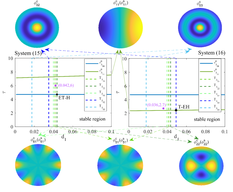
Figure 2: Partial bifurcation curves on the $d_{1}-\tau$ plane for two systems and eigenfuncitons related to Turing instability.

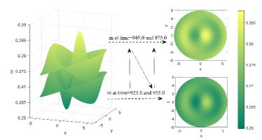
(a) (b)

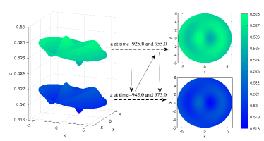
Figure 3: System (15) produces breathing patterns with parameters: $b=1.5,~{}\kappa=1,~{}\alpha=0.3,~{}R=6,~{}d_{1}=0.042,~{}\tau=6$. Initial values are $m(t,r,\theta)=0.2727+0.01\cdot\cos t\cdot\cos r\cdot\cos\theta,~{}a(t,r,\theta)=0.5238+0.01\cdot\cos t\cdot\cos r\cdot\cos\theta,~{}t\in[-\tau,0)$. $(a):m,~{}(b):a$.

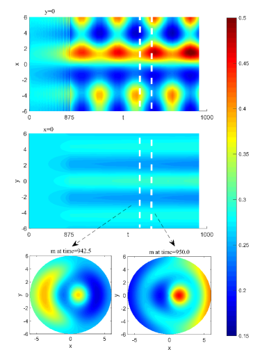
(a) (b)

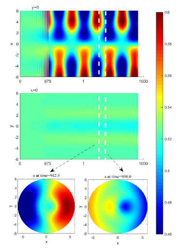
Figure 4: System (16) produces standing wave-like dynamic Turing-Hopf patterns with parameters: $b=1.5,~{}\kappa=1,~{}\alpha=0.3,~{}R=6,~{}d_{1}=0.036,~{}\tau=2.7$. Initial values are $m(t,r,\theta)=0.2727+0.01\cdot\cos t\cdot\cos r\cdot\cos\theta,~{}a(t,r,\theta)=0.5238+0.01\cdot\cos t\cdot\cos r\cdot\cos\theta,~{}t\in[-\tau,0)$. $(a):m,~{}(b):a$.

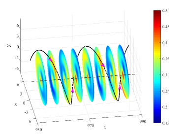
(a) (b)

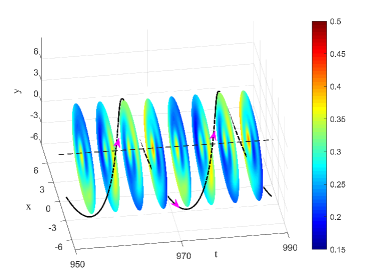
Figure 5: Rotating wave-like dynamic Turing-Hopf patterns of $m$ with parameters: $b=1.5,~{}\kappa=1,~{}\alpha=0.3,~{}R=6,~{}d_{1}=0.036,~{}\tau=2.7$. Initial values are $m(t,r,\theta)=0.2727+0.01\cdot\cos t\cdot\cos r\cdot\Theta_{1}(\theta),~{}a(t,r,\theta)=0.5238+0.01\cdot\cos t\cdot\cos r\cdot\Theta_{2}(\theta),~{}t\in[-\tau,0)$. $(a):(\Theta_{1}(\theta),\Theta_{2}(\theta))=(\cos\theta,\sin\theta)-clockwise,~{}(b):(\Theta_{1}(\theta),\Theta_{2}(\theta))=(\sin\theta,\cos\theta)-anticlockwise$.

V Concluding Remarks

In this paper, we investigate the interaction of Turing instability and Hopf bifurcation on a disk. We first present three Turing-Hopf normal forms based on different types of eigenspaces. In addition, we analyzed the possible solutions for each normal form, which can guide us to find solutions with physical significance in real-world systems. Finally, breathing, standing wave-like, and rotating wave-like patterns were simulated in a specific mussel-algae model.

Under the case (ET-EH), the possible solutions are complex, and there are several questions that can be further discussed. We believe that quasi-periodic solutions may also exist, which is quite difficult to study. In addition, in previous studies on double Hopf bifurcation, the resonance may occur: if the ratio of two imaginary roots $\mathrm{i}\omega_{1}$ and $\mathrm{i}\omega_{2}$ is rational, some additional terms cannot be eliminated. In this paper, another kind of resonance of Turing and Hopf appears, i.e. $n_{T_{3}}=2n_{H_{3}}$. Combining these factors and investigating the corresponding normal forms is a noteworthy issue to be further considered.

Appendix A The proof of Theorem III.1

In this section, we provide the decomposition of the phase space and the derivation of normal forms, by applying the method in (Faria, 2000; Song et al., 2016; Jiang et al., 2020), which leads to the results in Throrem III.1.

Let $\Lambda_{1}=\left\{\gamma:\Gamma_{0m_{1}}(\gamma)=0,~{}\mathrm{Re}{\gamma}=0\right\},~{}\Lambda_{2}=\left\{\gamma:\tilde{\Gamma}_{nm_{2}}(\gamma)=0,~{}\mathrm{Re}{\gamma}=0\right\}$. Define a bilinear pairing

$$(\psi,\varphi) =\int_{0}^{R}\int_{0}^{2\pi}r\left[\overline{\psi(0)}\varphi(0)-\int_{-\tau}^{0}\int_{\xi=0}^{\vartheta}\overline{\psi(\xi-\vartheta)}\mathrm{d}\eta(\hat{\nu},\vartheta)\varphi(\xi)\mathrm{d}\xi\right]\mathrm{d}r\mathrm{d}\theta,~{}\psi\in\left(\mathscr{C^{*}}\right)^{n},~{}\varphi\in\mathscr{C}^{n},$$ (17)

where $\left(\mathscr{C^{*}}\right)^{n}$ is the dual space of $\mathscr{C}^{n}$. By (Hale, 1977; Wu, 1996), one can decompose ${C}^{n}:=C([-1,0],\mathbb{C}^{n})$ by $\Lambda_{i}$ as

$${C}^{n}={P}_{i}\oplus{Q}_{i},~{}i=1,2,$$

where ${P}_{i}$ is the generalised eigenspace associated with $\Lambda_{i}$ and ${Q}_{i}=\{\phi\in\mathscr{C}:~{}\left(\psi,\phi\right)=0,~{}for~{}all~{}\psi\in{P}_{i}^{*}\}$. Here, ${P}_{i}^{*}$ is the dual space of ${P}_{i}$. Suitably, choose the bases $\Phi_{r\theta}^{i}$ and $\Psi_{r\theta}^{i}$ of ${P}_{i}$ and ${P}_{i}^{*}$, respectively, such that $\left(\Psi_{r\theta}^{i},\Phi_{r\theta}^{i}\right)=I_{n_{i}}$, where $n_{i}=\mathrm{dim}P_{i}$. Analogously, the phase space $\mathscr{C}^{n}$ can be decomposed as

$$\mathscr{C}^{n}=\mathscr{P}\oplus\mathscr{Q},~{}\mathscr{P}=\mathrm{Im}{\pi},~{}\mathscr{Q}=\mathrm{Ker}{\pi},$$ (18)

where $\mathrm{dim}{\mathscr{P}}=\sum_{i=1}^{2}{n_{i}}$, and $\pi:~{}\mathscr{X}\rightarrow\mathscr{P}$ is a projection defined by

$$\pi(U_{t})=\sum_{i=1}^{2}\left(\Phi_{r\theta}^{i}\langle\Psi_{r\theta}^{i},U_{t}\rangle\right)^{\mathrm{T}}.$$ (19)

In Table 1, we list roots with zero real part of the characteristic equation. By (ET-EH), we get that $\Lambda_{1}=\emptyset,~{}\Lambda_{2}=\{\pm\mathrm{i}\omega_{H_{3}},0\}$. Let

$$\Phi_{r\theta}^{2}= \left(\Phi^{2(1)}\cdot\hat{\phi}_{nm_{2}}^{c},~{}\Phi^{2(2)}\cdot\hat{\phi}_{nm_{2}}^{c},~{}\Phi^{2(3)}\cdot\hat{\phi}_{nm_{2}}^{s},~{}\Phi^{2(4)}\cdot\hat{\phi}_{nm_{2}}^{s},~{}\Phi^{2(5)}\cdot\hat{\phi}_{nm_{2}}^{c},~{}\Phi^{2(6)}\cdot\hat{\phi}_{nm_{2}}^{s}\right)$$

$$= \left(\xi_{H}\mathrm{e}^{\mathrm{i}\omega_{H_{3}}\vartheta}\hat{\phi}_{n_{H_{3}}m_{H_{3}}}^{c},~{}\overline{\xi_{H}}\mathrm{e}^{-\mathrm{i}\omega_{H_{3}}\vartheta}\hat{\phi}_{n_{H_{3}}m_{H_{3}}}^{c},~{}\xi_{H}\mathrm{e}^{\mathrm{i}\omega_{H_{3}}\vartheta}\hat{\phi}_{n_{H_{3}}m_{H_{3}}}^{s},~{}\overline{\xi_{H}}\mathrm{e}^{-\mathrm{i}\omega_{H_{3}}\vartheta}\hat{\phi}_{n_{H_{3}}m_{H_{3}}}^{s},\right.$$

$$\left.~{}~{}\xi_{T}\hat{\phi}_{n_{T_{3}}m_{T_{3}}}^{c},~{}{\xi_{T}}\hat{\phi}_{n_{T_{3}}m_{T_{3}}}^{s}\right),$$

$$\Psi_{r\theta}^{2}= \mathrm{col}\left(\Psi^{2(1)}\cdot\hat{\phi}_{nm_{2}}^{c},~{}\Psi^{2(2)}\cdot\hat{\phi}_{nm_{2}}^{c},~{}\Psi^{2(3)}\cdot\hat{\phi}_{nm_{2}}^{s},~{}\Psi^{2(4)}\cdot\hat{\phi}_{nm_{2}}^{s},~{}\Psi^{2(5)}\cdot\hat{\phi}_{nm_{2}}^{c},~{}\Psi^{2(6)}\cdot\hat{\phi}_{nm_{2}}^{s}\right)$$

$$= \mathrm{col}\left(\eta_{H}^{\mathrm{T}}\mathrm{e}^{\mathrm{i}\omega_{H_{3}}\varrho}\hat{\phi}_{n_{H_{3}}m_{H_{3}}}^{c},~{}\overline{\eta_{H}}^{\mathrm{T}}\mathrm{e}^{-\mathrm{i}\omega_{H_{3}}\varrho}\hat{\phi}_{n_{H_{3}}m_{H_{3}}}^{c},~{}\eta_{H}^{\mathrm{T}}\mathrm{e}^{\mathrm{i}\omega_{H_{3}}\varrho}\hat{\phi}_{n_{H_{3}}m_{H_{3}}}^{s},~{}\overline{\eta_{H}}^{\mathrm{T}}\mathrm{e}^{-\mathrm{i}\omega_{H_{3}}\varrho}\hat{\phi}_{n_{H_{3}}m_{H_{3}}}^{s}\right.$$

$$\left.~{}~{}~{}~{}~{}~{}~{}\eta_{T}^{\mathrm{T}}\hat{\phi}_{n_{T_{3}}m_{T_{3}}}^{c},~{}\eta_{T}^{\mathrm{T}}\hat{\phi}_{n_{T_{3}}m_{T_{3}}}^{s}\right),$$

where $\vartheta\in[-1,0),~{}\varrho\in(0,1]$, $\xi_{H}=(p_{11},p_{12},\cdots,p_{1n})^{\mathrm{T}}\in\mathbb{C}^{n}$ is the eigenvector associated with the eigenvalue $\mathrm{i}\omega$ and $\xi_{T}=(q_{11},q_{12},\cdots,q_{1n})^{\mathrm{T}}\in\mathbb{R}^{n}$ is the eigenvector associated with the eigenvalue 0. $\eta_{H}\in\mathbb{C}^{n}$ and $\eta_{T}\in\mathbb{R}^{n}$ are the corresponding adjoint eigenvectors that satisfy $\left(\Psi_{r\theta}^{2},\Phi_{r\theta}^{2}\right)=I_{6}.$

According to (19), $U_{t}=({u_{1}}_{t},{u_{2}}_{t},\cdots,{u_{n}}_{t})$ can be decomposed as

$$U_{t} =\left(\Phi_{r\theta}^{1}\langle\Psi_{r\theta}^{1},U_{t}\rangle\right)^{\mathrm{T}}+\left(\Phi_{r\theta}^{2}\langle\Psi_{r\theta}^{2},U_{t}\rangle\right)^{\mathrm{T}}+w_{t}$$ (20)

$$=\Phi_{r\theta}^{2}(z_{1},z_{2},z_{3},z_{4},z_{5},z_{6})^{\mathrm{T}}+w_{t}$$

$$=\Phi_{r\theta}z+w_{t},$$

with $\Phi_{r\theta}=\Phi_{r\theta}^{2},~{}z=(z_{1},z_{2},z_{3},z_{4},z_{5},z_{6})^{\mathrm{T}}$, and $w_{t}\in\mathscr{Q}$. Notice that the part $\Phi_{r\theta}^{2}(z_{1},z_{2},z_{3},z_{4},z_{5},z_{6})^{\mathrm{T}}$ stands for the solution on the center manifold, by which solutions on the center manifold are approximatively given.

It is easy to verify that

$$M_{j}^{1}(\mu^{l}z^{p}e_{k})=D_{z}(z^{p}\mu^{l}e_{k})Bz-Bz^{p}\mu^{l}e_{k}=\mathrm{i}\omega_{H_{3}}\left(p_{1}-p_{2}+(-1)^{k}\right)z^{p}\mu^{l}e_{k},~{}k=1,2,3,4$$ (21)

$$M_{j}^{1}(\mu^{l}z^{p}e_{k})=D_{z}(z^{p}\mu^{l}e_{k})Bz-Bz^{p}\mu^{l}e_{k}=\mathrm{i}\omega_{H_{3}}\left(p_{1}-p_{2}\right)z^{p}\mu^{l}e_{k},~{}k=5,6,$$

with $M_{j}^{1}$ defined in (Faria, 2000), ${B}=\mathrm{diag}\{\mathrm{i}\omega_{H_{3}},-\mathrm{i}\omega_{H_{3}},\mathrm{i}\omega_{H_{3}},-\mathrm{i}\omega_{H_{3}},0,0\}$, $j\geq 2,~{}z^{p}=z_{1}^{p_{1}}z_{2}^{p_{2}}z_{3}^{p_{3}}z_{4}^{p_{4}}z_{5}^{p_{5}}z_{6}^{p_{6}},~{}\mu^{l}=\mu_{1}^{l_{1}}\mu_{2}^{l_{2}},~{}p_{1}+p_{2}+p_{3}+p_{4}+l_{1}+l_{2}=j$, and $\{e_{1},e_{2},e_{3},e_{4},e_{5},e_{6}\}$ being the canonical basis for $\mathscr{C}^{6}$. Therefore,

$$\mathrm{Im}(M_{2}^{1})^{\mathrm{c}}=\mathrm{span} \left\{z_{1}z_{5}e_{1},z_{2}z_{5}e_{2},z_{3}z_{5}e_{3},z_{4}z_{5}e_{4},z_{3}z_{5}e_{1},z_{4}z_{5}e_{2},z_{1}z_{5}e_{3},z_{2}z_{5}e_{4},z_{5}^{2}e_{5},z_{6}^{2}e_{5},z_{5}z_{6}e_{5},\right.$$

$$\left.z_{1}z_{6}e_{1},z_{2}z_{6}e_{2},z_{3}z_{6}e_{3},z_{4}z_{6}e_{4},z_{3}z_{6}e_{1},z_{4}z_{6}e_{2},z_{1}z_{6}e_{3},z_{2}z_{6}e_{4},z_{5}^{2}e_{6},z_{6}^{2}e_{6},z_{5}z_{6}e_{6},\right.$$

$$\left.z_{1}\mu_{i}e_{1},z_{2}\mu_{i}e_{2},z_{3}\mu_{i}e_{3},z_{4}\mu_{i}e_{4},z_{3}\mu_{i}e_{1},z_{4}\mu_{i}e_{2},z_{1}\mu_{i}e_{3},z_{2}\mu_{i}e_{4},\right.$$

$$\left.z_{5}\mu_{i}e_{5},z_{5}\mu_{i}e_{6},z_{6}\mu_{i}e_{5},z_{6}\mu_{i}e_{6},\mu_{1}\mu_{2}e_{5},\mu_{i}^{2}e_{5},\mu_{1}\mu_{2}e_{6},\mu_{i}^{2}e_{6}\right\},$$

$$\mathrm{Im}(M_{3}^{1})^{\mathrm{c}}=\mathrm{span} \left\{z_{1}^{2}z_{2}e_{1},z_{3}^{2}z_{2}e_{1},z_{1}^{2}z_{4}e_{1},z_{3}^{2}z_{4}e_{1},z_{1}z_{5}^{2}e_{1},z_{1}z_{6}^{2}e_{1},z_{1}z_{5}z_{6}e_{1},z_{3}z_{5}^{2}e_{1},z_{3}z_{6}^{2}e_{1},z_{3}z_{5}z_{6}e_{1},\right.$$

$$\left.z_{1}\mu_{i}^{2}e_{1},z_{3}\mu_{i}^{2}e_{1},z_{1}z_{5}\mu_{i}e_{1},z_{1}z_{6}\mu_{i}e_{1},z_{3}z_{5}\mu_{i}e_{1},z_{3}z_{6}\mu_{i}e_{1},z_{1}\mu_{1}\mu_{2}e_{1},z_{3}\mu_{1}\mu_{2}e_{1},\right.$$

$$\left.z_{1}z_{2}z_{3}e_{1},z_{1}z_{3}z_{4}e_{1},\right.$$

$$\left.z_{1}^{2}z_{2}e_{3},z_{3}^{2}z_{2}e_{3},z_{1}^{2}z_{4}e_{3},z_{3}^{2}z_{4}e_{3},z_{1}z_{5}^{2}e_{3},z_{1}z_{6}^{2}e_{3},z_{1}z_{5}z_{6}e_{3},z_{3}z_{5}^{2}e_{3},z_{3}z_{6}^{2}e_{3},z_{3}z_{5}z_{6}e_{3},\right.$$

$$\left.z_{1}\mu_{i}^{2}e_{3},z_{3}\mu_{i}^{2}e_{3},z_{1}z_{5}\mu_{i}e_{3},z_{1}z_{6}\mu_{i}e_{3},z_{3}z_{5}\mu_{i}e_{3},z_{3}z_{6}\mu_{i}e_{3},z_{1}\mu_{1}\mu_{2}e_{3},z_{3}\mu_{1}\mu_{2}e_{3},\right.$$

$$\left.z_{1}z_{2}z_{3}e_{3},z_{1}z_{3}z_{4}e_{3},\right.$$

$$\left.z_{2}^{2}z_{1}e_{2},z_{4}^{2}z_{1}e_{2},z_{2}^{2}z_{3}e_{2},z_{4}^{2}z_{3}e_{2},z_{2}z_{5}^{2}e_{2},z_{2}z_{6}^{2}e_{2},z_{2}z_{5}z_{6}e_{2},z_{4}z_{5}^{2}e_{2},z_{4}z_{6}^{2}e_{2},z_{4}z_{5}z_{6}e_{2},\right.$$

$$\left.z_{2}\mu_{i}^{2}e_{2},z_{4}\mu_{i}^{2}e_{2},z_{2}z_{5}\mu_{i}e_{2},z_{2}z_{6}\mu_{i}e_{2},z_{4}z_{5}\mu_{i}e_{2},z_{4}z_{6}\mu_{i}e_{2},z_{2}\mu_{1}\mu_{2}e_{2},z_{4}\mu_{1}\mu_{2}e_{2},\right.$$

$$\left.z_{1}z_{2}z_{4}e_{2},z_{2}z_{3}z_{4}e_{2},\right.$$

$$\left.z_{2}^{2}z_{1}e_{4},z_{4}^{2}z_{1}e_{4},z_{2}^{2}z_{3}e_{4},z_{4}^{2}z_{3}e_{4},z_{2}z_{5}^{2}e_{4},z_{2}z_{6}^{2}e_{4},z_{2}z_{5}z_{6}e_{4},z_{4}z_{5}^{2}e_{4},z_{4}z_{6}^{2}e_{4},z_{4}z_{5}z_{6}e_{4},\right.$$

$$\left.z_{2}\mu_{i}^{2}e_{4},z_{4}\mu_{i}^{2}e_{4},z_{2}z_{5}\mu_{i}e_{4},z_{2}z_{6}\mu_{i}e_{4},z_{4}z_{5}\mu_{i}e_{4},z_{4}z_{6}\mu_{i}e_{4},z_{2}\mu_{1}\mu_{2}e_{4},z_{4}\mu_{1}\mu_{2}e_{4},\right.$$

$$\left.z_{1}z_{2}z_{4}e_{4},z_{2}z_{3}z_{4}e_{4},\right.$$

$$\left.z_{1}z_{2}z_{5}e_{5},z_{1}z_{4}z_{5}e_{5},z_{3}z_{2}z_{5}e_{5},z_{3}z_{4}z_{5}e_{5},z_{1}z_{2}z_{6}e_{5},z_{1}z_{4}z_{6}e_{5},z_{3}z_{2}z_{6}e_{5},z_{3}z_{4}z_{6}e_{5},\right.$$

$$\left.z_{1}z_{2}\mu_{i}e_{5},z_{1}z_{4}\mu_{i}e_{5},z_{3}z_{2}\mu_{i}e_{5},z_{3}z_{4}\mu_{i}e_{5},z_{5}\mu_{i}^{2}e_{5},z_{5}\mu_{1}\mu_{2}e_{5},z_{6}\mu_{i}^{2}e_{5},z_{6}\mu_{1}\mu_{2}e_{5},\right.$$

$$\left.z_{5}^{3}e_{5},z_{6}^{3}e_{5},z_{5}^{2}z_{6}e_{5},z_{6}^{2}z_{5}e_{5},\mu_{i}^{3}e_{5},\mu_{1}^{2}\mu_{2}e_{5},\mu_{1}\mu_{2}^{2}e_{5},\right.$$

$$\left.z_{1}z_{2}z_{5}e_{6},z_{1}z_{4}z_{5}e_{6},z_{3}z_{2}z_{5}e_{6},z_{3}z_{4}z_{5}e_{6},z_{1}z_{2}z_{6}e_{6},z_{1}z_{4}z_{6}e_{6},z_{3}z_{2}z_{6}e_{6},z_{3}z_{4}z_{6}e_{6},\right.$$

$$\left.z_{1}z_{2}\mu_{i}e_{6},z_{1}z_{4}\mu_{i}e_{6},z_{3}z_{2}\mu_{i}e_{6},z_{3}z_{4}\mu_{i}e_{6},z_{5}\mu_{i}^{2}e_{6},z_{5}\mu_{1}\mu_{2}e_{6},z_{6}\mu_{i}^{2}e_{6},z_{6}\mu_{1}\mu_{2}e_{6},\right.$$

$$\left.z_{5}^{3}e_{6},z_{6}^{3}e_{6},z_{5}^{2}z_{6}e_{6},z_{6}^{2}z_{5}e_{6},\mu_{i}^{3}e_{6},\mu_{1}^{2}\mu_{2}e_{6},\mu_{1}\mu_{2}^{2}e_{6}\right\},$$

In fact, according to (Song et al., 2016), the normal forms for Turing-Hopf bifurcation has the following form

$$\dot{z}={B}_{1}z+\frac{1}{2!}g_{2}^{1}(z,0,\mu)+\frac{1}{3!}g_{3}^{1}(z,0,0)+o(|z||\mu|^{2}).$$ (22)

where $g_{2}^{1}(z,0,\mu)$ and $g_{3}^{1}(z,0,0)$ are defined in (Song et al., 2016). By the analysis in (Chen et al., 2023; Faria, 2000; Song et al., 2016), noticing the fact

$$\int_{0}^{R}\int_{0}^{2\pi}r\left(\hat{\phi}_{n_{H_{3}}m_{H_{3}}}^{c}\right)^{k_{1}}\left(\hat{\phi}_{n_{H_{3}}m_{H_{3}}}^{s}\right)^{k_{2}}\left(\hat{\phi}_{n_{T_{3}}m_{T_{3}}}^{c}\right)^{k_{3}}\left(\hat{\phi}_{n_{T_{3}}m_{T_{3}}}^{s}\right)^{k_{4}}\mathrm{d}\theta\mathrm{d}r\left\{\begin{array}[]{cc}\neq 0,&k_{1}n_{H_{3}}-k_{2}n_{H_{3}}+k_{3}n_{T_{3}}-k_{4}n_{T_{3}}=0,\\ =0,&others,\end{array}\right.$$

and the relationship of $\Phi_{r\theta}$ and $\Psi_{r\theta}$, we obtain that when $n_{T_{3}}\neq 2n_{H_{3}}$, the normal forms truncated to the third order for ET-EH bifurcation can be summarized as

$$\dot{z}_{1}= \mathrm{i}\omega_{H_{3}}z_{1}+B_{11}\mu_{1}z_{1}+B_{21}\mu_{2}z_{1}+B_{100020}z_{1}z_{5}^{2}+B_{001020}z_{3}z_{5}^{2}+B_{100002}z_{1}z_{6}^{2}+B_{001002}z_{3}z_{6}^{2}$$ (23)

$$+B_{210000}z_{1}^{2}z_{2}+B_{200100}z_{1}^{2}z_{4}+B_{012000}z_{3}^{2}z_{2}+B_{002100}z_{3}^{2}z_{4}+B_{111000}z_{1}z_{2}z_{3}+B_{101100}z_{1}z_{3}z_{4}$$

$$+B_{100011}z_{1}z_{5}z_{6}+B_{001011}z_{3}z_{5}z_{6},$$

$$\dot{z}_{2}= -\mathrm{i}\omega_{H_{3}}z_{2}+\overline{B_{11}}\mu_{1}z_{2}+\overline{B_{21}}\mu_{2}z_{2}+\overline{B_{100020}}z_{2}z_{6}^{2}+\overline{B_{001020}}z_{4}z_{6}^{2}+\overline{B_{100002}}z_{2}z_{5}^{2}+\overline{B_{001002}}z_{4}z_{5}^{2}$$

$$+\overline{B_{210000}}z_{1}z_{2}^{2}+\overline{B_{200100}}z_{2}^{2}z_{3}+\overline{B_{012000}}z_{4}^{2}z_{1}+\overline{B_{002100}}z_{4}^{2}z_{3}+\overline{B_{111000}}z_{1}z_{2}z_{4}+\overline{B_{101100}}z_{2}z_{3}z_{4},$$

$$+\overline{B_{100011}}z_{2}z_{5}z_{6}+\overline{B_{001011}}z_{2}z_{5}z_{6},$$

$$\dot{z}_{3}= \mathrm{i}\omega_{H_{3}}z_{3}+B_{11}\mu_{1}z_{3}+B_{21}\mu_{2}z_{3}+B_{100020}z_{3}z_{5}^{2}+B_{001020}z_{1}z_{5}^{2}+B_{100002}z_{3}z_{6}^{2}+B_{001002}z_{1}z_{6}^{2}$$

$$+B_{210000}z_{3}^{2}z_{4}+B_{200100}z_{3}^{2}z_{2}+B_{012000}z_{1}^{2}z_{4}+B_{002100}z_{1}^{2}z_{2}+B_{111000}z_{1}z_{3}z_{4}+B_{101100}z_{1}z_{2}z_{3},$$

$$+B_{100011}z_{3}z_{5}z_{6}+B_{001011}z_{1}z_{5}z_{6},$$

$$\dot{z}_{4}= -\mathrm{i}\omega_{H_{3}}z_{4}+\overline{B_{11}}\mu_{1}z_{4}+\overline{B_{21}}\mu_{2}z_{2}+\overline{B_{10002}}z_{4}z_{6}^{2}+\overline{B_{00102}}z_{2}z_{6}^{2}+\overline{B_{100002}}z_{4}z_{5}^{2}+\overline{B_{001002}}z_{2}z_{5}^{2}$$

$$+\overline{B_{21000}}z_{3}z_{4}^{2}+\overline{B_{20010}}z_{4}^{2}z_{1}+\overline{B_{01200}}z_{2}^{2}z_{3}+\overline{B_{00210}}z_{1}^{2}z_{2}+\overline{B_{11100}}z_{2}z_{3}z_{4}+\overline{B_{10110}}z_{1}z_{2}z_{4},$$

$$+\overline{B_{100002}}z_{4}z_{6}^{2}+\overline{B_{001002}}z_{2}z_{6}^{2}$$

$$\dot{z}_{5}= B_{15}\mu_{1}z_{5}+B_{25}\mu_{2}z_{5}+B_{110010}z_{1}z_{2}z_{5}+B_{100110}z_{1}z_{4}z_{5}+B_{011010}z_{2}z_{3}z_{5}+B_{001110}z_{3}z_{4}z_{5}$$

$$+B_{110001}z_{1}z_{2}z_{6}+B_{100101}z_{1}z_{4}z_{6}+B_{011001}z_{2}z_{3}z_{6}+B_{001101}z_{3}z_{4}z_{6}$$

$$+B_{000030}z_{5}^{3}+B_{000003}z_{6}^{3}+B_{000021}z_{5}^{2}z_{6}+B_{000012}z_{5}z_{6}^{2},$$

$$\dot{z}_{6}= B_{15}\mu_{1}z_{6}+B_{25}\mu_{2}z_{6}+B_{110010}z_{1}z_{2}z_{6}+B_{100110}z_{1}z_{4}z_{6}+B_{011010}z_{2}z_{3}z_{6}+B_{001110}z_{3}z_{4}z_{6}$$

$$+B_{110001}z_{1}z_{2}z_{5}+B_{100101}z_{1}z_{4}z_{5}+B_{011001}z_{2}z_{3}z_{5}+B_{001101}z_{3}z_{4}z_{5}$$

$$+B_{000030}z_{6}^{3}+B_{000003}z_{5}^{3}+B_{000021}z_{6}^{2}z_{5}+B_{000012}z_{6}z_{5}^{2}.$$

By (van Gils and Mallet-Paret, 1986), after a sequence of local invertible transformations, the normal form truncated to the third order can be reduced to

$$\dot{z}_{1}=\mathrm{i}\omega_{H_{3}}z_{1}+B_{11}\mu_{1}z_{1}+B_{21}\mu_{2}z_{1}+B_{200100}z_{1}^{2}z_{4}+B_{111000}z_{1}z_{2}z_{3}+B_{100011}z_{1}z_{5}z_{6},$$ (24)

$$\dot{z}_{2}=-\mathrm{i}\omega_{H_{3}}z_{2}+\overline{B_{11}}\mu_{1}z_{2}+\overline{B_{21}}\mu_{2}z_{2}+\overline{B_{200100}}z_{3}z_{2}^{2}+\overline{B_{111000}}z_{1}z_{2}z_{4}+\overline{B_{100011}}z_{2}z_{5}z_{6},$$

$$\dot{z}_{3}=\mathrm{i}\omega_{H_{3}}z_{3}+B_{11}\mu_{1}z_{3}+B_{21}\mu_{2}z_{3}+B_{200100}z_{3}^{2}z_{2}+B_{111000}z_{1}z_{3}z_{4}+B_{100011}z_{3}z_{5}z_{6},$$

$$\dot{z}_{4}=-\mathrm{i}\omega_{H_{3}}z_{4}+\overline{B_{11}}\mu_{1}z_{4}+\overline{B_{21}}\mu_{2}z_{4}+\overline{B_{200100}}z_{1}z_{4}^{2}+\overline{B_{111000}}z_{2}z_{3}z_{4}+\overline{B_{100011}}z_{4}z_{5}z_{6},$$

$$\dot{z}_{5}=B_{15}\mu_{1}z_{5}+B_{25}\mu_{2}z_{5}+B_{100110}z_{1}z_{4}z_{5}+B_{011010}z_{2}z_{3}z_{5}+B_{000021}z_{5}^{2}z_{6},$$

$$\dot{z}_{6}=B_{15}\mu_{1}z_{6}+B_{25}\mu_{2}z_{6}+B_{100110}z_{1}z_{4}z_{6}+B_{011010}z_{2}z_{3}z_{6}+B_{000021}z_{5}z_{6}^{2}.$$

The proof is similar to Lemma III.2 of (Chen et al., 2023).

Through the change of variables

$$\begin{array}[]{lll}z_{1}=\rho_{H^{1}}\mathrm{e}^{\mathrm{i}\chi_{H^{1}}},{}&z_{4}=\rho_{H^{1}}\mathrm{e}^{-\mathrm{i}\chi_{H^{1}}},\\ z_{3}=\rho_{H^{2}}\mathrm{e}^{\mathrm{i}\chi_{H^{2}}},{}&z_{2}=\rho_{H^{2}}\mathrm{e}^{-\mathrm{i}\chi_{H^{2}}},\\ z_{5}=\rho_{T^{1}},{}&z_{6}=\rho_{T^{2}},\end{array}$$ (25)

we obtain (5) with

$$\epsilon_{1}(\mu)=\mathrm{Re}\{B_{11}\}\mu_{1} +\mathrm{Re}\{B_{21}\}\mu_{2},~{}\epsilon_{2}(\mu)=B_{15}\mu_{1}+B_{25}\mu_{2},$$

$$c_{11}=\mathrm{Re}\{B_{200100}\},{} c_{12}=\mathrm{Re}\{B_{111000}\},~{}c_{13}=\mathrm{Re}\{B_{100011}\},$$

$$c_{21}=B_{100110},{} c_{22}={B_{011010}},~{}c_{23}={B_{000021}}.$$

References

- Camara et al. (2016) B. I. Camara, M. Haque, and H. Mokrani, Physica A: Statistical Mechanics and its Applications 461, 374 (2016).
- Yang and Song (2016) R. Yang and Y. Song, Nonlinear Analysis: Real World Applications 31, 356 (2016).
- Cao and Jiang (2018) X. Cao and W. Jiang, Nonlinear Analysis: Real World Applications 43, 428 (2018).
- Kumari and Mohan (2020) N. Kumari and N. Mohan, Nonlinear Dynamics 100, 763 (2020).
- Kumar and Gangopadhyay (2020) P. Kumar and G. Gangopadhyay, Physical Review E 101, 042204 (2020).
- Cross and Hohenberg (1993) M. C. Cross and P. C. Hohenberg, Review of Modern Physics 65, 851 (1993).
- Perraud et al. (1993) J. J. Perraud, A. De Wit, E. Dulos, P. De Kepper, G. Dewel, and P. Borckmans, Physical Review Letters 71, 1272 (1993).
- Heidemann et al. (1993) G. Heidemann, M. Bode, and H. G. Purwins, Physics Letters A 177, 225 (1993).
- Vallette et al. (1994) D. P. Vallette, W. S. Edwards, and J. P. Gollub, Physical Review E 49, R4783 (1994).
- Song and Zou (2014) Y. Song and X. Zou, Computers & Mathematics with Applications 67, 1978 (2014).
- An and Jiang (2018) Q. An and W. Jiang, International Journal of Bifurcation and Chaos 28, 1850108 (2018).
- Rovinsky and Menzinger (1992) A. Rovinsky and M. Menzinger, Physical Review A 46, 6315 (1992).
- Meixner et al. (1997) M. Meixner, A. De Wit, S. Bose, and E. Schöll, Physical Review E 55, 6690 (1997).
- Bose et al. (2000) S. Bose, P. Rodin, and E. Schöll, Physical Review E 62, 1778 (2000).
- Baurmann et al. (2007) M. Baurmann, T. Gross, and U. Feudel, Journal of Theoretical Biology 245, 220 (2007).
- Just et al. (2001) W. Just, M. Bose, S. Bose, H. Engel, and E. Schöll, Physical Review E 64, 026219 (2001).
- Venkov et al. (2007) N. A. Venkov, S. Coombes, and P. C. Matthews, Physica D: Nonlinear Phenomena 232, 1 (2007).
- Ledesma-Durán and Aragón (2020) A. Ledesma-Durán and J. L. Aragón, Communications in Nonlinear Science and Numerical Simulation 83, 105145 (2020).
- Song et al. (2016) Y. Song, T. Zhang, and Y. Peng, Communications in Nonlinear Science and Numerical Simulation 33, 229 (2016).
- Jiang et al. (2020) W. Jiang, Q. An, and J. Shi, Journal of Differential Equations 268, 6067 (2020).
- Song et al. (2019) Y. Song, H. Jiang, and Y. Yuan, Journal of Applied Analysis and Computation 9, 1132 (2019).
- Wu and Zhao (2020) D. Wu and H. Zhao, Journal of Nonlinear Science 30, 1015 (2020).
- Lv (2021) Y. Lv, Nonlinear Dynamics 107, 1357 (2021).
- Duan et al. (2022) D. Duan, B. Niu, and J. Wei, Discrete and Continuous Dynamical Systems-Series B 27, 3683 (2022).
- Chen et al. (2021) M. Chen, R. Wu, H. Liu, and X. Fu, Chaos, Solitons & Fractals 153, 111509 (2021).
- Abid et al. (2015) W. Abid, R. Yafia, M. Aziz-Alaoui, H. Bouhafaa, and A. Abichoua, Applied Mathematics and Computation 260, 292 (2015).
- Paquin-Lefebvre et al. (2019) F. Paquin-Lefebvre, W. Nagata, and M. J. Ward, SIAM Journal on Applied Dynamical Systems 18, 1334 (2019).
- Golubitsky et al. (1989) M. Golubitsky, I. Stewart, and D. G. Schaeffer, Singularities and Groups in Bifurcation Theory: Volume II (Springer-Verlag, New York, 1989).
- Guo and Wu (2013) S. Guo and J. Wu, Bifurcation Theory of Functional Differential Equations (Springer-Verlag, New York, 2013).
- Hale (1977) J. K. Hale, Theory of Functional Differential Equations (Springer-Verlag, New York, 1977).
- Wu (1996) J. Wu, Theory and Applications of Partial Functional Differential Equations (Springer-Verlag, New York, 1996).
- Murray (2001) J. D. Murray, Mathematical Biology II: Spatial Models and Biomedical Applications (Springer-Verlag, New York, 2001).
- Pinchover and Rubinstein (2005) Y. Pinchover and J. Rubinstein, An Introduction to Partial Differential Equations (Cambridge University Press, 2005).
- Chen et al. (2023) Y. Chen, X. Zeng, and B. Niu, “Equivariant Hopf bifurcation in a class of partial functional differential equations on a circular domain,” (2023), arXiv:2305.05979 [math.DS] .
- Guckenheimer and Holmes (1983) J. Guckenheimer and P. Holmes, Nonlinear Oscillations, Dynamical Systems, and Bifurcations of Vector Fields (Springer-Verlag, New York, 1983).
- Shen and Wei (2019) Z. Shen and J. Wei, International Journal of Bifurcation and Chaos 29, 1950144 (2019).
- Steen (2003) H. Steen, Botanica Marina 46, 36 (2003).
- Manoylov (2009) K. M. Manoylov, Journal of Freshwater Ecology 24, 145 (2009).
- Faria (2000) T. Faria, Transactions of the American Mathematical Society 352, 2217 (2000).
- van Gils and Mallet-Paret (1986) S. A. van Gils and J. Mallet-Paret, Proceedings of the Royal Society of Edinburgh Section A: Mathematics 104, 279 (1986).