Inspection planning under execution uncertainty

Abstract

Autonomous inspection tasks necessitate effective path-planning mechanisms to efficiently gather observations from points of interest (POI). However, localization errors commonly encountered in urban environments can introduce execution uncertainty, posing challenges to the successful completion of such tasks. To tackle these challenges, we present IRIS-under uncertainty (IRIS-U²), an extension of the incremental random inspection-roadmap search (IRIS) algorithm, that addresses the offline planning problem via an A*-based approach, where the planning process occurs prior the online execution. The key insight behind IRIS-U² is transforming the computed localization uncertainty, obtained through Monte Carlo (MC) sampling, into a POI probability. IRIS-U² offers insights into the expected performance of the execution task by providing confidence intervals (CI) for the expected coverage, expected path length, and collision probability, which becomes progressively tighter as the number of MC samples increase. The efficacy of IRIS-U² is demonstrated through a case study focusing on structural inspections of bridges. Our approach exhibits improved expected coverage, reduced collision probability, and yields increasingly-precise CIs as the number of MC samples grows. Furthermore, we emphasize the potential advantages of computing bounded sub-optimal solutions to reduce computation time while still maintaining the same CI boundaries.

I Introduction and related work

We consider the problem of planning in an offline phase a collision-free path for a robot to inspect a set of points of interest (POIs) using onboard sensors. This can be a challenging task, especially in urban environments as dynamics (e.g., control constraints) and localization errors (e.g., inaccuracies in location estimates) increase the task’s complexity. In particular, localization can be a significant source of uncertainty in urban environments, leading to missed POIs and compromising the efficiency and accuracy of inspection missions.

One application that motivates this work is the inspection of bridges using unmanned aerial vehicles (UAVs) [1]. Almost $40\%$ of the bridges in the United States of America exceed their $50$-year design life [2], and regular inspections are critical to ensuring bridge safety. UAVs, or drones, can be used to efficiently inspect the bridge structure, allowing it to be visually assessed at close range without the need for human inspectors to walk across the deck or utilize under-bridge inspection units [3]. In such settings, the UAV is usually equipped with a camera to inspect the POIs, and a navigation system to determine its location. The navigation system typically fuses information from different sensors such as a global navigation satellite system (GNSS) and inertial sensors. However, GNSS signals can be blocked or distorted by the bridge, leading to location inaccuracies that rely mainly on inertial measurements and can compromise the effectiveness of the inspection mission (see Fig. 1).

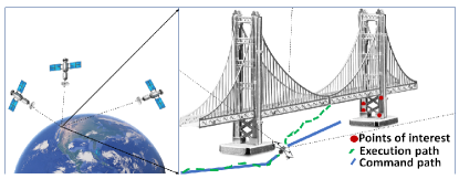
Figure 1: A UAV executing a bridge-inspection task, following a command path pre-computed offline (dark blue). The UAV relies on GNSS satellite signals for navigation but the bridge obstructs one satellite signal during a particular segment of its path (light blue), leading to a substantial deviation from the command path. This deviation hinders the UAV’s ability to inspect the desired POIs and may result in a collision with the bridge.

In this study, we aim to address the problem of offline path planning for inspection tasks in urban environments, where uncertainty during mission execution can lead to missed POIs. Our objective is to devise a method that can pre-compute a path before the inspection mission begins, which serves as a command path robust enough to accommodate uncertainties during execution.

Several approaches have been proposed to perform inspection planning without accounting for uncertainty. Some algorithms decompose the region containing the POIs into sub-regions and solve for each sub-region separately [4], while others divide the problem into two NP-hard problems: (i) solving the art gallery problem to compute a small set of viewpoints that collectively observe all the POIs, and (ii) solving the traveling salesman problem to compute the shortest path to visit this set of viewpoints [5, 6, 7, 8]. Another common approach is to simultaneously compute both inspection points (i.e., points from which POIs are inspected) and the trajectory to visit these inspection points using sampling-based techniques [9, 10]. However, these approaches do not consider the execution uncertainty, which can lead to missed POIs due to differences between the path executed and the path planned.

Using these methods for planning with low uncertainty can be done using an upgraded navigation system that does not rely on GNSS, such as RF tools like WIFI [11], Bluetooth [12], or acoustic waves [13], or more expensive and heavy sensors like mobile LIDAR mapping [14], or tactical grade inertial sensors and RTK/dGNSS [15]. However, these solutions may require a supportive communication infrastructure or more expensive and heavy sensors.

Various approaches have been proposed to address localization uncertainty for safe path planning (which only considers a motion between states without inspection points). For instance, minimum-distance collision-free paths can be computed while bounding the uncertainty by, e.g., a self-localization error ellipsoid, or uncertainty corridor [16, 17, 18]. Another approach [19], uses a mixed-observability Markov decision process approach to account for a-priori probabilistic sensor availability and path execution error propagation. Englot et al. [20] suggest an RRT*-based method which minimizes the maximum path segment of the uncertainty metric encountered during the path traversal. Sampling-based planners that explicitly reason about the evolution of the robot’s belief have also been proposed [21, 22, 23, 24].

However, when it comes to localization uncertainty in inspection tasks, additional challenges arise due to the uncertainty of inspecting the POIs. Papachristos et al. [8] proposed a planner that propagates the covariance matrix of the extended Kalman filter (EKF) to maintain a belief state about the robot’s location and the POI inspected. However, while this approach excels in online scenarios where it can utilize real-time measurements, it may encounter challenges in offline inspection planning where the planning process occurs before the actual execution. Specifically, the covariance matrix is established based on a specific online scenario, utilizing received GNSS signals, and it characterizes the extent of uncertainty associated with the localization process tied that of a particular signal. Consequently, this uncertainty may encompass areas where GNSS outages are anticipated but not pertinent within the context of that specific scenario. However, when transitioning from an offline planning phase to an execution phase, there’s a possibility that new localization errors can emerge, distinct from those encountered during the offline planning phase and potentially compromising the inspection task.

This leads to our main insight: We can maximize POI inspection by transforming the computed localization uncertainty, derived via Monte Carlo (MC) sampling, into a POI probability. This transformed probability then serves as the optimization objective for the algorithm. Here, we rely on the incremental random inspection-roadmap search (IRIS) algorithm [25] which naturally allows us to maximize POI inspection. We extend the algorithm to consider POI uncertainty resulting in a new algorithm which we term IRIS-under uncertainty (IRIS-U²). IRIS-U² considers a variety of possible paths produced by MC samples and estimates the POI inspection probability, the collision probability, and the path length of the execution phase.

Using MC sampling, IRIS-U² estimates with a certain confidence level (CL) the desired performance criteria (i.e., path length, coverage, and collision probabilities) within some confidence interval (CI) depending on the number of the MC samples used [26]. However, when selecting an execution path from multiple optional paths, straightforward statistical analysis may be biased toward false negatives and either require offline prepossessing to provide guarantees or should be used as guidelines (see details in Appendix D). We choose the latter approach and outline a procedure to set a user-defined parameter for providing a CI, which becomes tighter as the number of samples increases and which becomes true asymptotically. Additionally, we highlight the potential benefits of using a bounded sub-optimal solution in certain situations to reduce computation time while still providing guarantees through the CI boundaries.

We demonstrate the effectiveness of IRIS-U² through a simulated case study of structural inspections of bridges using a UAV in an urban environment. Our results show that IRIS-U² is able to achieve a desired level of coverage, while also reducing collision probability and tightening the CI lower boundaries as the number of MC samples increases.

The rest of this paper is organized as follows. In Sec. II, we formulate the problem of offline path planning for inspection tasks under execution uncertainty. In Sec. III, we describe the algorithmic background and in Sec. IV we describe our proposed approach in detail. Then in Sec. VI and VII we present the results of our simulated experiments. Finally, in Sec. VIII, we summarize our main contributions and discuss future work.

II Problem Definition

In this section, we provide a formal definition of the inspection-planning problem under execution uncertainty. We start by introducing basic definitions and notations, and discuss the uncertainity considerations (Sec. II-A). Next, we formally describe the inspection-planning problem in the deterministic (uncertainity-free) regime (Sec. II-B). Then, we introduce the inspection-planning problem under execution uncertainty which will be the focus of this work (Sec. II-C).

II-A Basic definitions and notations

We have a holonomic robot $\mathcal{R}$ operating in a workspace $\mathcal{W}\subset~{}\mathbb{R}^{3}$ amidst a set of (known) obstacles $\mathcal{W}_{\rm obs}\subset\mathcal{W}$. A configuration $q$ is a $d$-dimensional vector uniquely describing the robot’s pose (position and orientation) and let $\mathcal{X}\subset\mathbb{R}^{d}$ denote the robot’s configuration space.  Let $\text{Shape}:\mathcal{X}\rightarrow 2^{\mathcal{W}}$ be a function mapping a configuration $q$ to the workspace region occupied by $\mathcal{R}$ when placed at $q$ (here, $2^{\mathcal{W}}$ is the power set of $\mathcal{W}$). We say that $q\in\mathcal{X}$ is collision free if $\text{Shape}(q)\bigcap\mathcal{W}_{obs}=\emptyset$.

A path $\pi=(q_{0},q_{1},\ldots)\subset\mathcal{X}$ is a sequence of configurations called milestones connected by straight-line edges $\overline{q_{i}q_{i+1}}$. A path $\pi$ is collision free if every configuration along the path (i.e., either one of the milestones or along the edges connecting milestones) is collision-free. We use the binary function $\mathcal{C}(\pi)$ to express the collision state of a path $\pi$ where $\mathcal{C}(\pi)=0$ and $\mathcal{C}(\pi)=1$ correspond to $\pi$ being collision free and in-collision, respectively. Finally, we use $\ell(\pi)$ to denote the length of a given path $\pi$.

When a path $\pi$ is computed in an offline phase to be later executed by the robot, we refer to it as a command path. Unfortunately, when following the command path, the system typically deviates from $\pi$ due to different sources of uncertainty. In particular, we assume that the robot operates under two sources of uncertainty: (i) control uncertainty and (ii) localization uncertainty. A simple toy example demonstrating these concepts is detailed in Sec. IV.

The control uncertainty could result from various sources, such as a mismatch between the robot model used during planning and the real robot model, and disturbances in the environment (e.g., wind gusts). When attempting to follow the pre-computed command path $\pi$, even in the absence of localization uncertainty, control uncertainty could result in deviations of the robot from $\pi$ [27].

Localization uncertainty (which is usually the main source of uncertainty in an urban environment) corresponds to navigation-model parameters that determine the robot’s configuration which is not accurately known. Those parameters need to be modeled as random variables and may include biases of the inertial sensors or GNSS error terms [28].

To this end, we assume that we have access to distributions $\mathcal{D}_{\rm unc}$ from which the parameter governing the execution uncertainty $\mathcal{N}_{\rm unc}$ is drawn (see example in Sec. IV-B1).. In addition, we assume to have access to the initial true location (i.e., there is no uncertainty in the initial configuration of any execution path regardless of the command path provided). Finally, we assume that we have access to a black-box simulator of a motion model $\mathcal{M}$ that, given a command-path $\pi$ the uncertainty parameters $\mathcal{N}_{\rm unc}$ and the initial location outputs the path that the robot will pursue starting from the initial location while following $\pi$ assuming uncertainty parameters $\mathcal{N}_{\rm unc}$. Note that after $\mathcal{N}_{\rm unc}$ is drawn, the model is deterministic.

II-B Inspection planning (without execution uncertainty)

In the inspection-planning problem, we receive as input a set of POI $\mathcal{I}=\{\iota_{1},\ldots,\iota_{k}\}\subset\mathcal{W}$ which should be inspected using some on-board inspection sensors (e.g., a camera). We model the inspection sensors as a mapping $\mathcal{S}:\mathcal{X}\rightarrow 2^{\mathcal{I}}$ such that $\mathcal{S}(q)$ denotes the subset of $\mathcal{I}$ that are inspected from a configuration $q\in\mathcal{X}$. By a slight abuse of notation, we define $\mathcal{S}(\pi):=\bigcup_{i}\mathcal{S}(q_{i})$ to be the POI that can be inspected by traversing the path $\pi=(q_{0},q_{1},\ldots)$. For simplicity, we only inspect POIs along milestones (rather than edges). We start with a simplified setting of the inspection problem which involves no uncertainty on the side of controls or localization. That is, a robot performing the inspection can precisely follow a path during execution time and its location is known exactly. Such a setting was solved by IRIS (see Sec. III-A).

Problem 1 (Deterministic problem)

In the inspection-planning problem we wish to compute in an offline phase a path $\pi$ that maximizes its coverage $|{\mathcal{S}}(\pi)|$. Out of all such paths we wish to compute the paths whose length ${\ell}(\pi)$ is minimal.

Note. In practice, one may be interested in minimizing mission completion time or energy consumption (and not path length which is a first-order approximation for these metrics). Optimizing for these metrics is slightly more complex and is left for future work.

Prob. 1 can be defined for the continuous setting (i.e., when we consider all paths in $\mathcal{X}$ between a given start configuration $q_{\rm start}$ and goal configuration $q_{\rm goal}$) or for the discrete setting where we restrict the set of available paths to those defined via a given roadmap. Here, a roadmap $\mathcal{G}=(\mathcal{V},\mathcal{E})$ is a graph embedded in the configuration space $\mathcal{X}$ such that each vertex is associated with a configuration and each edge with a local path connecting close-by configurations. Roadmaps are commonly used in motion-planning algorithms (see, e.g., [31, 32]) and, as we will see, will be the focus of this work as well.

II-C Inspection-planning problem under execution uncertainty

In the inspection-planning problem under execution uncertainty, we calculate a command-path $\pi$ in an offline stage. To account for localization and control uncertainty when executing $\pi$, the following definitions extend the notion of path length, path coverage, and collision state to be their expected values:

Definition 1

The expected collision, coverage, and length probabilities are defined as:

$$\bar{\mathcal{C}}(\pi) :=E_{\mathcal{N}_{\rm unc}\sim\mathcal{D}_{\rm unc}}\left[\mathcal{C}\left(\mathcal{M}(\pi,\mathcal{N}_{\rm unc})\right)\right],$$ (1a)

$$|\bar{\mathcal{S}}(\pi)| :=E_{\mathcal{N}_{\rm unc}\sim\mathcal{D}_{\rm unc}}\left[|\mathcal{S}\left(\mathcal{M}(\pi,\mathcal{N}_{\rm unc})\right)|\right],$$ (1b)

$$\bar{\ell}(\pi) :=E_{\mathcal{N}_{\rm unc}\sim\mathcal{D}_{\rm unc}}\left[\ell\left(\mathcal{M}(\pi,\mathcal{N}_{\rm unc})\right)\right],$$ (1c)

respectively. Here, $\bar{\mathcal{C}}(\pi)\in\left[0,1\right]$, where $\bar{\mathcal{C}}(\pi)=0$ and $\bar{\mathcal{C}}(\pi)=1$ correspond to $\pi$ being guaranteed to be collision-free and in-collision, respectively.

We are now ready to formally introduce the optimal inspection-planning problem under execution uncertainty.

Problem 2 (Optimal problem)

In the optimal inspection-planning problem under execution uncertainty we are given a user-provided threshold $\rho_{\text{coll}}\in[0,1]$ and we wish to compute in an offline phase a command-path $\pi$ such that its expected execution collision probability is below $\rho_{\text{coll}}$ (i.e., $\bar{\mathcal{C}}(\pi)\leq\rho_{\text{coll}}$), and which maximizes the expected coverage $|\bar{\mathcal{S}}(\pi)|$. Of all such paths, we wish to choose the one whose expected length $\bar{\ell}(\pi)$ is minimal.

Finally, we introduce a relaxation of the above problem to reduce its computational cost.

Problem 3 (Sub-optimal problem)

Let $\pi^{*}$ be the solution to the optimal inspection-planning problem under uncertainty. In addition, let $\varepsilon\geq 0$, and $\kappa\in(0,1]$ be user-provided approximation factors with respect to path length and coverage, respectively. Then, in the sub-optimal inspection-planning problem under execution uncertainty we wish to compute in an offline phase a command path $\pi$ such that:

$$\bar{\mathcal{C}}(\pi)\leq \rho_{\text{coll}},$$ (2a)

$$|\bar{\mathcal{S}}(\pi)|\geq \kappa\cdot|{\mathcal{S}}(\pi^{*})|,$$ (2b)

$$\bar{\ell}(\pi)\leq (1+\varepsilon)\cdot{\ell}(\pi^{*}).$$ (2c)

Notice that, by setting $\kappa=1$ and $\varepsilon=0$ the sub-optimal Prob. 3 is equivalent to Prob. 2. Unfortunately, as we are only given a black-box model of $\mathcal{M}$, it is infeasible to directly compute the expected values for coverage, collision probability, and length, $|\bar{\mathcal{S}}(\pi)|$, $\bar{\mathcal{C}}(\pi)$ and $\bar{\ell}(\pi)$, respectively. As we will see, our approach will be to solve Prob. 3 using estimates of these values.

III Algorithmic background

In this section, we provide algorithmic background. We begin by describing IRIS [25], a state-of-the-art algorithm for solving the continuous inspection-planning problem in the deterministic regime (Prob. 1). We then continue to outline the statistical methods we will use. Throughout the text we assume familiarity with the A* algorithm [33].

III-A Incremental Random Inspection-roadmap Search (IRIS)

IRIS solves Prob. 1 by incrementally constructing a sequence of increasingly dense graphs, or roadmaps, embedded in $\mathcal{X}$ and computes an inspection plan over the roadmaps as they are constructed. The roadmap $\mathcal{G}=(\mathcal{V},E)$ is a Rapidly-exploring Random Graph (RRG) [34] rooted at the start configuration (though other types of graphs, such as PRM*, can be used as well). For simplicity, when describing IRIS below (and IRIS-U² later on), we focus on the behavior of the algorithm for a given roadmap. More information on how to construct such roadmaps can be found in [25].

Let $\mathcal{I}_{\mathcal{G}}:=\{\iota\in\mathcal{I}|\exists v\in\mathcal{V}\text{ s.t. }\iota\in\mathcal{S}(v)\}$ be the set of all inspection points that can be inspected from some roadmap vertex. To compute an inspection plan, IRIS considers the inspection graph $\mathcal{G}_{\mathcal{S}}=(\mathcal{V}_{\mathcal{S}},\mathcal{E}_{\mathcal{S}})$ induced by the roadmap $\mathcal{G}$. Here, vertices are pairs comprised of a vertex $u\in\mathcal{V}$ in the roadmap $\mathcal{G}$ and subsets of $\mathcal{I}_{\mathcal{G}}$. Namely, $\mathcal{V}_{\mathcal{S}}=\mathcal{V}\times 2^{\mathcal{I}_{\mathcal{G}}}$, and note that $|\mathcal{V}_{\mathcal{S}}|=O\left(|\mathcal{V}|\cdot 2^{|\mathcal{I}_{\mathcal{G}}|}\right)$. An edge $e\in\mathcal{E}_{\mathcal{S}}$ between vertices $(u,\mathcal{I}_{u})$ and $(v,\mathcal{I}_{v})$ exists if $(u,v)\in\mathcal{E}$ and $\mathcal{I}_{u}\cup\mathcal{S}(v)=\mathcal{I}_{v}$. The cost of such an edge is simply the the length of the edge $(u,v)\in\mathcal{E}$, namely $\ell(u,v)$. The graph $\mathcal{G}_{\mathcal{S}}$ has the property that a shortest path in the inspection graph corresponds to an optimal inspection path $\pi^{*}$ over $\mathcal{G}$. However, the size of $\mathcal{G}_{\mathcal{S}}$ is exponential in the number of POIs $|\mathcal{I}_{\mathcal{G}}|$. Thus, to reduce the runtime complexity IRIS uses a search algorithm that approximates $\pi^{*}$, which allows to prune the search space of paths over $\mathcal{G}_{\mathcal{S}}$.

Specifically, the powerful approach for pruning the search space used by IRIS is through the notion of approximate dominance, which allows to only consider paths that can significantly improve the quality (either in terms of length or the set of points inspected) of a given path. In particular, let $\pi,\pi^{\prime}$ be two paths in $\mathcal{G}$ that start and end at the same vertices and let $\varepsilon\geq 0$ and $\kappa\in(0,1]$ be some approximation parameters. We say that $\pi$ $(\varepsilon,\kappa)$-dominates $\pi^{\prime}$ if $\ell(\pi)\leq(1+\varepsilon)\cdot\ell(\pi^{\prime})$ and $|\mathcal{S}(\pi)|\geq\kappa\cdot|\mathcal{S}(\pi)\cup\mathcal{S}(\pi^{\prime})|$. If $\pi$ indeed $(\varepsilon,\kappa)$-dominates $\pi^{\prime}$ then $\pi^{\prime}$ can potentially be pruned. However, if we prune away approximate-dominated paths, we need to efficiently account for all paths that were pruned away in order to bound the quality of the solution obtained. This is done through the notion of potentially-achievable paths described below.

The search algorithm used by IRIS employs an A*-like search over $\mathcal{G}_{\mathcal{S}}$, where each node in the search tree is associated with a path pair (PP) corresponding to a vertex $v$ in $\mathcal{G}_{\mathcal{S}}$ (rather than only a path). Here, a PP is a tuple $(\pi,\tilde{\pi})$, where $\pi$ and $\tilde{\pi}$ are the so-called achievable path (AP) and potentially achievable path (PAP), respectively. The AP $\pi$ represents a realizable path in $\mathcal{G}_{\mathcal{S}}$, from the start vertex to $v$, and is associated with two scalars corresponding to the path’s length and coverage, respectively. The PAP $\tilde{\pi}$ is a pair of scalars $\tilde{\ell},\tilde{S}$ representing length and coverage, respectively, which are used to bound the quality of any achievable paths to $v$ represented by a specific PP. Note that $\tilde{\pi}$ does not imply necessarily that there exists any path $\pi^{\prime}$ from from the start to $v$ such that $\ell(\pi^{\prime})=\ell(\tilde{\pi})$ and $\mathcal{S}(\pi)=\mathcal{S}(\tilde{\pi})$. It merely states that such a path could exist.

A PP is said to be $(\varepsilon,\kappa)$-bounded if (i) the length of the AP is no more than $(1+\varepsilon)$ times the length of the PAP and (ii) the coverage of the PAP is at least $\kappa$ percent of the coverage of the AP.

The search algorithm starts with a path pair rooted at the start vertex $v_{\rm start}$ where both the AP and the PAP represent the trivial paths that only contain $v_{\rm start}$ (i.e., the scalars associated with the length of the AP and the PAP are zero and the scalars associated with the coverage of the AP and the PAP is $\mathcal{S}(v_{\rm start})$). It operates in a manner similar to A*, with an OPEN list and a CLOSED set to track nodes that have not and have been considered, respectively. Each iteration begins with popping a node from the OPEN list and checking if an inspection path has been found. If this is not the case, the popped node from the OPEN list is inserted into the CLOSED set and the iteration continues.

The next step is extending this node and testing whether its successors are dominated by an existing node. If this is the case, the node is discarded. Otherwise, IRIS tests whether the node can be subsumed by or subsume another node.

These three core operations (extending, dominating, and subsuming) are key to the efficiency of IRIS. When extending a node, a path pair $\textsf{PP}_{u}=(\pi_{u},\tilde{\pi}_{u})$ to some vertex $u$ is extended by an edge $e=(u,v)\in\mathcal{E}_{\mathcal{S}}$ to create the path pair $\textsf{PP}_{v}=(\pi_{v},\tilde{\pi}_{v})$. The length and coverage of the AP of $\pi_{u}$ are defined by $\ell(\pi_{u})+\ell(e)$ and $\mathcal{S}(\pi_{u})\cup\mathcal{S}(v)$, respectively. Similarly, the length and coverage of the PAP $\tilde{\pi}_{v}$ are $\ell(\tilde{\pi}_{v})+\ell(e)$ and $\mathcal{S}(\tilde{\pi}_{u})\cup\mathcal{S}(\tilde{\pi}_{v})$, respectively. When testing domination, two path pairs $\textsf{PP}_{u,1}$ and $\textsf{PP}_{u,2}$ to some vertex $u\in\mathcal{V}_{\mathcal{S}}$ are considered. $\textsf{PP}_{u,1}$ is said to dominate $\textsf{PP}_{u,2}$ if both $\ell(\pi_{u,1})\leq\ell(\pi_{u,2})$ and $\mathcal{S}(\pi_{u,2})\subseteq\mathcal{S}(\pi_{u,1})$. In such a case, $\textsf{PP}_{u,1}$ is preferable to $\textsf{PP}_{u,2}$ and so $\textsf{PP}_{u,2}$ can be discarded. However, in many settings two path pairs will not dominate each other but their respective path lengths and coverage will be similar. To avoid maintaining and extending such similar path pairs, IRIS uses the subsuming operation. This operation is denoted by $\textsf{PP}_{u,1}\oplus\textsf{PP}_{u,2}$, which creates a new path pair $\textsf{PP}_{u,3}$ whose AP’s length and coverage are identical to those of $\textsf{PP}_{u,1}$. The PAP’s length of $\textsf{PP}_{u,3}$ is the minimum PAP’s length of $\textsf{PP}_{1},\textsf{PP}_{2}$, and the PAP’s coverage is the union of the coverage of the PAPs of $\textsf{PP}_{1}$ and $\textsf{PP}_{2}$. Subsuming is only performed as long as the resultant PP is $(\varepsilon,\kappa)$-bounded which allows to guarantee bounds on the solution quality. For additional details, see [25].

The algorithm’s asymptotic convergence to an optimal solution is achieved through a process of iterative roadmap densification and parameter tightening. This iterative approach involves systematically refining the roadmap $\mathcal{G}$ (i.e., adding vertices and edges) while progressively reducing the parameters $\varepsilon$ and $\kappa$. Roadmap densification ensures that the algorithm considers larger sets of configurations, leading to more accurate and refined solutions. Meanwhile, the tightening of parameters focuses the algorithm on increasingly promising paths within the roadmap.

III-B Monte-Carlo methods & confidence intervals

Monte Carlo methods are a family of statistical techniques used to simulate and analyze complex systems that involve randomness. These methods involve generating multiple random samples and using them to estimate the value of a process being studied. Due to the finite number of samples, there is uncertainty regarding the true value of the process. To quantify this uncertainty, a common approach is CI and CL [26, 35].

A CI is a range of values likely to contain the true value of a population’s parameter (such as its mean) with a certain confidence levels. For example, in our setting this could be the expected path length. The size of the CI reflects the uncertainty around the estimated value and is influenced by the number of samples used. As the number of samples increases, the accuracy of the estimate improves (i.e., CL increases) and the CI decreases. See additional background on the statistical tools we use in Appendix A.

IV Method

In this section, we present our method called IRIS under uncertainty, or IRIS-U², to solve Prob. 3. This is done by extending the algorithmic framework of IRIS to consider execution uncertainty within the inspection-planning algorithm. We start with a general description of our algorithmic approach (Sec. IV-A), and then describe how the operations used in IRIS are modified to account for localization uncertainty (Sec. IV-B). We conclude by describing how those updated operations are used by IRIS-U² to compute an inspection path (Sec. IV-C).

IV-A IRIS-U²—Algorithmic approach

A naïve approach to address execution uncertainty is to penalize paths with high localization uncertainty. We describe one such approach as a baseline in Sec. VI-B. As we will see, while highly efficient in collision avoidance, even minor deviations from the command path due to execution uncertainty can lead to discrepancies between the intended POI coverage of the command path and the actual path taken during execution, particularly when obstacles are present. Thus, instead of reasoning about localization uncertainty, in IRIS-U², we directly consider and maximize POI coverage.

Unfortunately, we cannot directly compute the expected values for coverage, collision probability, and length, $|\bar{\mathcal{S}}(\pi)|$, $\bar{\mathcal{C}}(\pi)$ and $\bar{\ell}(\pi)$, respectively. Thus, we tackle Prob. 3 using the estimated values $\hat{\mathcal{S}}(\pi),\hat{\mathcal{C}}(\pi)$ and $\hat{\ell}(\pi)$ instead of the expectation values $|\bar{\mathcal{S}}(\pi)|,\bar{\mathcal{C}}(\pi)$ and $\bar{\ell}(\pi)$ such that the command path $\pi$, satisfies:

$$\hat{\mathcal{C}}(\pi)\leq \rho_{\text{coll}},$$ (3a)

$$|\bar{\mathcal{S}}(\pi)|\geq \kappa\cdot|\hat{\mathcal{S}}(\pi^{*})|,$$ (3b)

$$\bar{\ell}(\pi)\leq (1+\varepsilon)\cdot\hat{\ell}(\pi^{*}).$$ (3c)

Here, the estimated coverage $\hat{\mathcal{S}}(\pi)$, the estimated collision probability $\hat{\mathcal{C}}(\pi)$ and the estimated path length $\hat{\ell}(\pi)$ are computed by simulating $m\geq 1$ different executions (with respect to uncertainty) of $\pi$ (see details below).

Similar to IRIS, IRIS-U² solves the inspection-planning problem by sampling an initial roadmap. It then iteratively (i) plans a command path on this roadmap and (ii) densifies the roadmap and refines the algorithm’s parameters. Importantly, the focus of this work is on the path-planning part of the algorithmic framework wherein a command path is computed for a given roadmap. This is visualized in Fig. 2 where the path-planning part is highlighted. For completeness, we reiterate that graph refinement is done by continuing to grow the RRG as described in Sec. III.

Figure 2: Planning a command path $\pi$ to inspect set of POI $\mathcal{I}$ given the input of IRIS— $\mathcal{G}$, $\kappa$ and $\varepsilon$, and the additional parameters of IRIS-U²— $m$ the $\rho_{\text{coll}}$.

Specifically, we start by initializing our algorithm by sampling $m$ different parameters $\mathcal{N}_{\rm unc}^{1},\ldots,\mathcal{N}_{\rm unc}^{m}$ from $\mathcal{D}_{\rm unc}$. For any command path $\pi$ considered by the algorithm, we will estimate $\bar{\ell}(\pi)$ and $\bar{\mathcal{S}}(\pi)$ by simulating $m$ execution paths $\pi^{e}_{1},\ldots,\pi^{e}_{m}$ using the $m$ motion models. Namely,

$$\pi^{e}_{i}:=\mathcal{M}(\pi,\mathcal{N}_{\rm unc}^{i}).$$ (4)

To estimate the expected coverage, let $\xi_{i,j}\in\{0,1\}$ be a variable that will be set to one if path $\pi^{e}_{i}$ covers the $j$’th POI. Namely,

$$\xi_{i,j}:=\begin{cases}1&\iota_{j}\in\mathcal{S}(\pi^{e}_{i}),\\ 0&\text{else}.\end{cases}$$ (5)

Then, we define for the command path $\pi$ the inspection probability vector (IPV):

$$\textup{IPV}(\pi):=\{\hat{p}_{1}^{\pi},\ldots,\hat{p}_{k}^{\pi}\}.$$ (6)

where:

$$\hat{p}_{j}^{\pi}:=\frac{1}{m}\sum_{i=1}^{i=m}\xi_{i,j},$$ (7)

is the estimated probability that the $j$’th POI is viewed when executing the command path $\pi$. Finally, the estimated expected coverage is defined as:

$$|\hat{\mathcal{S}}(\pi)|:=\sum_{j=1}^{j=k}\hat{p}^{\pi}_{j}.$$ (8)

Assumption 1

Here, we assume that the probability $\hat{p}^{\pi}_{j}$ of inspecting each POI $j$ is independent of other POIs.

As we will see, Assumption 1 will both (i) simplify the analysis and (ii) will not hinder the guarantees obtained from the analysis in practice. Relaxing the assumption is left for future work.

To estimate the collision probability $\hat{\mathcal{C}}(\pi)$ of a path $\pi$, IRIS-U² maintains for the command path $\pi$ a collision vector (CV):

$$\rm{CV}(\pi):=\{\zeta_{1}^{\pi},\zeta_{2}^{\pi},\ldots\}.$$ (9)

Here, $\zeta_{j}^{\pi}$ indicates whether the path $\pi_{j}^{e}$ was found to be in a collision. Namely:

$$\zeta_{j}^{\pi}:=\begin{cases}1&\pi_{j}^{e}~{}\text{is in collision},\\ 0&\text{else}.\end{cases}$$ (10)

Subsequently, the estimated collision probability $\hat{\mathcal{C}}(\pi)$ of a path $\pi$ is defined as:

$$\hat{\mathcal{C}}(\pi):=\frac{1}{m}\sum_{j=1}^{j=m}\zeta_{j}^{\pi}.$$ (11)

Similarly, the estimated expected path length $\bar{\ell}(\pi)$ is defined as:

$$\hat{\ell}(\pi):=\frac{1}{m}\sum_{j=1}^{j=m}\ell~{}(\pi^{e}_{j}).$$ (12)

IV-B IRIS-U²—Modified search operations

Recall that, while IRIS maintains the POIs inspected using a set representation, IRIS-U² maintains an inspection probability vector (IPV) for each path. In addition, IRIS-U² maintains estimations of the expected path length and expected collision probability of its command path. This requires to modify the node’s operations used by IRIS’s search algorithm to account for the uncertainty values. Next we will explain how to modify the operations used in IRIS-U²’s A*-like search that were originally used in IRIS. We start by introducing a toy problem that will be used as running example in Sec. IV-B1. Then, we formally define nodes in Sec. IV-B2 and detail the node extension, collision, and domination operations in Sec. IV-B3, IV-B4 and IV-B5. Finally, we describe the node subsuming operation in Sec. IV-B6 and termination criteria in Sec. IV-B7.

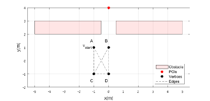
Figure 3: Toy scenario for running example with one POI (red dot), two obstacles (red rectangles), and four vertices (black dots) connected with six edges (black dashed lines).

IV-B1 Toy problem

Consider the toy problem illustrated in Fig. 3. The roadmap $\mathcal{G}$ contains four vertices $A$, $B$, $C$, and $D$ which represent configurations of a point robot (namely, each configuration defines the location $(x,y)$ of the point robot). Here, we assume that the single POI can be seen from any configuration as long as the straight-line connecting them does not intersect an obstacle.

Here, we use a simple toy motion model $\mathcal{M}_{\text{toy}}$ to define the execution localization uncertainty in which we assume that the position of every configuration along the command path is normally distributed around the position of the corresponding configuration. Specifically, parameters $\mathcal{N}_{\rm unc}:=(r,\theta)$ are drawn from the distribution $\mathcal{D}_{\rm unc}$ such that $r\sim|\mathcal{N}(0,1)|$, and $\theta\sim\mathcal{N}(0,2\pi)$. Now, given a command path $\pi^{c}$ with $n>1$ configurations $\pi^{c}=\{\langle x_{1}^{c},y_{1}^{c}\rangle,\ldots\langle x_{n}^{c},y_{n}^{c}\rangle\}$, the corresponding executed path (which is also a random variable) is $\pi_{e}=\{\langle x_{1}^{e},y_{1}^{e}\rangle,\ldots\langle x_{n}^{e},y_{n}^{e}\rangle\}$ such that $x_{i}^{e}=x_{i}^{c}+r\cdot\cos\theta$ and $y_{i}^{e}=y_{i}^{c}+r\cdot\sin\theta$ for $i>1$.

Note that (i) as we assume that there is no uncertainty in the initial location, $\langle x_{1}^{c},y_{1}^{c}\rangle=\langle x_{1}^{e},y_{1}^{e}\rangle$ and that (ii) in contrast to the general setting, here uncertainty is only a function of the current configuration and not of the entire command path.

Finally, in the running example, we assume that the algorithm uses three MC planning samples $(m=3)$ and the start configuration is located at vertex $A$.

IV-B2 Node definition

A node $n$ in our search algorithm is a tuple:

$$n=\langle u,\pi_{u},\Pi^{e}_{u},\hat{\rm{IPV}}_{u},\hat{\ell}_{u},\tilde{\rm{IPV}}_{u},\tilde{\ell}_{u},\hat{\mathcal{C}}_{u}\rangle,$$ (13)

where $u\in\mathcal{V}$ is a roadmap vertex, $\pi_{u}$ is a path from the start vertex $v_{\rm start}\in\mathcal{G}$ to $u$, $\Pi_{u}^{e}=\{\pi_{1,u}^{e},\ldots,\pi_{m,u}^{e}\}$ are $m$ simulated execution paths calculated using Eq. (4), $\hat{\rm{IPV}}_{u}=\{\hat{p}_{1}^{\pi_{u}},\ldots,\hat{p}_{k}^{\pi_{u}}\}$ is the estimated IPV (see Eq. (6)), and $\hat{\ell}_{u}$ is the estimated path length (see Eq. (12)) with respect to the command path $\pi_{u}$. In addition, $\tilde{\textup{IPV}}_{u}=\{\hat{p}_{1}^{\tilde{\pi}_{u}},\ldots,\hat{p}_{k}^{\tilde{\pi}_{u}}\}$ and $\tilde{\ell}_{u}$ are the estimated IPV and estimated length of the PAP. Finally, $\hat{\mathcal{C}}_{u}$ is the estimated collision probability of $\pi_{u}$ (see Eq. (11)).

We define the initial node as:

$$n_{\text{init}}:=\langle v_{\rm start},\{v_{\rm start}\},\Pi^{e}_{v_{\rm start}},\text{IPV}_{v_{\rm start}},0,\text{IPV}_{v_{\rm start}},0,0\rangle,$$ (14)

where the command path $\pi$ of $n_{\text{init}}$ consists of the trivial path starting and ending at $v_{\rm start}$ whose estimated length and collision are initialized to zero (we assume that $v_{\rm start}$ corresponds to a collision-free configuration). In addition, the $m$ MC starting configurations are set to be $v_{\rm start}$ (namely, $\Pi^{e}_{v_{\rm start}}=\{v_{\rm start},\ldots,v_{\rm start}\}$) which induce the initial inspection probability vector $\text{IPV}_{v_{\rm start}}=\{\mathcal{S}(v_{\rm start}),\ldots,\mathcal{S}(v_{\rm start})\}$. Finally, analogously to IRIS, the IPV and estimated length of the PAP are initialized to be the same as the AP.

Example 1

For the running example, the first location of each MC planning sample is at $v_{\rm start}$ and the POI cannot be inspected from that location. Specifically, $n_{\text{init}}$ is defined such that:

$$v_{\rm start}= A,$$

$$\Pi^{e}_{v_{\rm start}}= \{\langle-1,1\rangle;\langle-1,1\rangle;\langle-1,1\rangle\},$$

$$\text{IPV}_{v_{\rm start}}= \{\hat{p}_{1}^{\pi_{v_{\rm start}}}\}=\{0\}.$$

IV-B3 Node extension

Let $u,v\in\mathcal{V}$ be two roadmap vertices such that $(u,v)\in\mathcal{E}$. and let $n_{u}=\langle u,\pi_{u},\Pi^{e}_{u},\hat{\rm{IPV}}_{u},\hat{\ell}_{u},\tilde{\rm{IPV}}_{u},\tilde{\ell}_{u},\hat{\mathcal{C}}_{u}\rangle$ be a node in the search algorithm associated with vertex $u$. We define the operation of extending $n_{u}$ by the edge $(u,v)$ as creating a new node $n_{v}=\langle v,\pi_{v},\Pi^{e}_{v},\hat{\rm{IPV}}_{v},\hat{\ell}_{v},\tilde{\rm{IPV}}_{v},\tilde{\ell}_{v},\hat{\mathcal{C}}_{v}\rangle$ such that:

• $\pi_{v}$ is the result of concatenating $\pi_{v}$ with the path $\pi_{u\rightarrow v}$ from $u$ to $v$. Namely,

  $$\pi_{v}:=\pi_{u}\circ\pi_{u\rightarrow v}.$$ (15)

• $\Pi^{e}_{v}:=\{\pi_{1,v}^{e}\ldots\pi_{m,v}^{e}\}$ is a set of execution paths such that $\pi^{e}_{j,v}:=\mathcal{M}(\pi_{v},\mathcal{N}_{\rm unc}^{j})$. Notice that this can be efficiently computed by denoting:

  $$\pi^{e}_{j,u\rightarrow v}:=\mathcal{M}(\pi_{u\rightarrow v},\mathcal{N}_{\rm unc}^{j},\pi^{e}_{j,u}),$$ (16)

  and setting:

  $$\pi^{e}_{j,v}:=\pi^{e}_{j,u}\circ\pi^{e}_{j,u\rightarrow v}.$$ (17)

• $\hat{\rm{IPV}}_{v}:=\{\hat{p}_{1}^{\pi_{v}},\ldots,\hat{p}_{k}^{\pi_{v}}\}$ is obtained by leveraging the assumptions, that (i) POI inspections are conducted at vertices (see Sec. II-A) and that (ii) each inspection is independent (see Assumption. 1).

  $$\forall j\in[1,m]~{}\hat{p}_{j}^{\pi_{v}}:=1-(1-\hat{p}^{\pi_{u\rightarrow v}}_{j})\cdot~{}(1-\hat{p}_{j}^{\pi_{u}}).$$ (18)

• $\hat{\ell}_{v}$ is the estimated path length of $\pi_{v}$. Notice that this can be efficiently computed by setting:

  $$\hat{\ell}_{v}:=\hat{\ell}_{u}+\hat{\ell}(\pi_{u\rightarrow v}).$$ (19)

• The estimated IPV of the PAP is updated such that:

  $$\forall j\in[1,m]~{}\tilde{p}_{j}^{\pi_{v}}:=1-(1-\hat{p}^{\pi_{u\rightarrow v}}_{j})\cdot~{}(1-\hat{p}_{j}^{\tilde{\pi}_{u}}).$$ (20)

  and the estimated path length of the PAP is:

  $$\tilde{\ell}_{v}:=\tilde{\ell}_{u}+\hat{\ell}(\pi_{u\rightarrow v}).$$ (21)

• $\hat{\mathcal{C}}_{v}$ is the collision probability of node $v$, such that:

  $$\hat{\mathcal{C}}_{v}:=1-\left(1-\hat{\mathcal{C}}_{u}\right)\cdot\left(1-\hat{\mathcal{C}}_{u\rightarrow v}\right).$$ (22)

Example 2

Extending the node $n_{\text{init}}$ defined in Ex. 1 by edge $e(A,B)$ will result in a new node:

$$n_{B}=\langle B,\pi_{B},\Pi^{e}_{B},\hat{\rm{IPV}}_{B},\hat{\ell}_{B},\tilde{\rm{IPV}}_{B},\tilde{\ell}_{B},\hat{\mathcal{C}}_{B}\rangle,$$

where $\pi_{B}=\{A,B\}$ and $\Pi^{e}_{B}$ is calculated using $\mathcal{M}_{\text{toy}}$ to be:

$$\Pi^{e}_{B}=\{ \langle-1,1\rangle,\langle 0.6,2.1\rangle;$$

$$\langle-1,1\rangle,\langle 0.5,1.2\rangle;$$

$$\langle-1,1\rangle,\langle-0.2,1.6\rangle\}.$$

As a result, since POI $1$ can only be seen from $\Pi^{e}_{B,2}$ and $\Pi^{e}_{B,3}$, then $\hat{p}^{\pi_{A\rightarrow B}}_{1}\cong 0.67$. Using these values, we can calculate $\hat{p}_{1}^{\pi_{B}}$ and $\hat{p}_{1}^{\tilde{\pi}_{B}}$ as:

$$\hat{p}_{1}^{\pi_{B}}= 1-(1-\hat{p}^{\pi_{A\rightarrow B}}_{1})\cdot(1-\hat{p}_{1}^{\pi_{A}})=$$

$$= 1-(1-0.67)\cdot(1-0)=0.67,$$

$$\hat{p}_{1}^{\tilde{\pi}_{B}}= \max(\hat{p}^{\pi_{A\rightarrow B}}_{1},\hat{p}_{1}^{\tilde{\pi}_{A}})=0.67.$$

Thus, $\hat{\rm{IPV}}_{B}=\tilde{\rm{IPV}}_{B}=0.67$. As $\hat{\ell}(\pi_{u\rightarrow v})\cong 1.48$ (using $\Pi^{e}_{B}$), we have that $\hat{\ell}_{B}=\tilde{\ell}_{B}=0+1.48$. Finally, $\Pi^{e}_{B,1}$ collides with the middle obstacle, and $\hat{\mathcal{C}}_{B}=\frac{1}{3}$.

IV-B4 Node collision

Recall that the collision probability of a node estimates the probability that the command path associated with $n$ will intersect an obstacle. Now, let $n_{u}=\langle u,\pi_{u},\Pi^{e}_{u},\hat{\rm{IPV}}_{u},\hat{\ell}_{u},\tilde{\rm{IPV}}_{u},\tilde{\ell}_{u},\hat{\mathcal{C}}_{u}\rangle$ be a node in the search algorithm associated with vertex $u$. Then, given a user-defined threshold $\rho_{\text{coll}}\in[0,1]$ a node $n$ will be considered in collision (and hence pruned by the search) if its collision probability $\hat{\mathcal{C}}_{u}$ satisfies $\hat{\mathcal{C}}_{u}\geq\rho_{\text{coll}}$.

Example 3

Assuming $\rho_{\text{coll}}=0$ (i.e., we only allow collision-free paths), then in Ex. 2, $\hat{\mathcal{C}}_{B}=\frac{1}{3}\geq\rho_{\text{coll}}$ is considered in collision and this extension is discarded.

IV-B5 Node domination

As in many A*-like algorithms, node domination is used to prune away nodes that cannot improve the solution compared to other nodes expanded by the algorithm. We introduce a similar notion that accounts for both converge (via IPVs) and path length.

Specifically, let $n_{1}$ and $n_{2}$ be two nodes that start at $v_{\text{start}}\in\mathcal{V}$ and end at the same vertex $u\in\mathcal{V}$. Here, we assume that for each $i\in\{1,2\}$,

$$n_{i}=\langle u,\pi_{u,i},\Pi^{e}_{u,i},\hat{\rm{IPV}}_{u,i},\hat{\ell}_{u,i},\tilde{\rm{IPV}}_{u,i},\tilde{\ell}_{u,i},\hat{\mathcal{C}}_{u}\rangle.$$ (23)

Then, we say that $n_{1}$ dominates $n_{2}$ if:

$$\forall j\in[1\ldots k],~{}\hat{p}_{j}^{\tilde{\pi}_{1}}\geq\hat{p}_{j}^{\tilde{\pi}_{2}}\quad\text{and}\quad\hat{\ell}(\tilde{\pi}_{1})\leq\hat{\ell}(\tilde{\pi}_{2}).$$ (24)

Example 4

Assume that node $n_{{D},1}$ represents the command path $A\mbox{-}D$ in the running example and its IPV and estimated length of the AP and the PAP are:

$$\hat{\rm{IPV}}_{{D},1}=\{0.67\},\quad \hat{\ell}_{{D},1}=2.4$$

$$\tilde{\rm{IPV}}_{{D},1}=\{0.67\},\quad \tilde{\ell}_{{D},1}=2.4.$$

In addition, assume that later in the search node $n_{{D},2}$ represents another command path $A\mbox{-}C\mbox{-}D$. This path also reached vertex $D$ and its IPV and estimated length of the AP and the PAP are:

$$\hat{\rm{IPV}}_{{D},2}=\{0.77\},\quad \hat{\ell}_{{D},2}=2.9$$

$$\tilde{\rm{IPV}}_{{D},2}=\{0.77\},\quad \tilde{\ell}_{{D},2}=2.9.$$

Here, the estimated length of $2.9$ is the sum of the estimated lengths of $A\mbox{-}C$ and $C\mbox{-}D$. In addition, the IPV of the AP and PAP contains a probability of $0.33$ to inspect the POI from vertex $C$ and $0.67$ to inspect it from vertex $D$. Thus, the value of $\hat{\rm{IPV}}_{{D},2}$ equals $1-(1-0.67)\cdot(1-0.33)\cong 0.77$ (using Eq. (18)). Similarly, the value of $\tilde{\rm{IPV}}_{{D},2}$ is also equal to $0.77$. Notice that, the path lengths and IPVs of the AP and PAP are identical here. This will change shortly when we introduce node subsuming (Sec IV-B6).

Here, despite that $\tilde{\ell}_{{D},1}=2.4\leq 2.9=\tilde{\ell}_{{D},2}$ (namely, the path to $n_{D,1}$ is shorter than the path to $n_{D,2}$), we have that $\hat{p}_{1}^{\tilde{\pi}_{{D},1}}=0.67\leq 0.77=\hat{p}_{1}^{\tilde{\pi}_{{D},2}}$ (namely, the path to $n_{D,1}$ has a smaller probability of inspecting the POI). Thus, $n_{{D},1}$ does not dominates $n_{{D},2}$.

IV-B6 $(\varepsilon,\kappa)$-bounded nodes & node subsuming

Similar to IRIS, we need to ensure that the PAP bounds the AP given the user-provided parameters $\varepsilon>0$ and $\kappa\in[0,1]$. Specifically, let $n_{u}=\langle u,\pi_{u},\Pi^{e}_{u},\hat{\rm{IPV}}_{u},\hat{\ell}_{u},\tilde{\rm{IPV}}_{u},\tilde{\ell}_{u},\hat{\mathcal{C}}_{u}\rangle$ be a node such that $\hat{\rm{IPV}}(\pi_{u}):=\{\hat{p}_{1}^{\pi_{u}},\ldots,\hat{p}_{k}^{\pi_{u}}\}$ and $\tilde{\rm{IPV}}(\pi_{u}):=\{\tilde{p}_{1}^{\pi_{u}},\ldots,\tilde{p}_{k}^{\pi_{u}}\}$ are the IPVs of $n$’s AP and PAP, respectively. Similarly, let $\hat{\ell}_{u}$ and $\tilde{\ell}_{u}$ be the estimated lengths of $n$’s AP and PAP, respectively. We say that $n$ is $(\varepsilon,\kappa)$-bounded if:

$$\sum_{j=1}^{j=k}\hat{p}_{j}^{\pi_{u}}\geq\kappa\cdot\sum_{j=1}^{j=k}\hat{p}_{j}^{{\pi}_{u}}\quad\text{and}\quad\hat{\ell}_{u}\leq~{}(1+\varepsilon)\cdot\tilde{\ell}_{u}.$$ (25)

Similar to IRIS, $(\varepsilon,\kappa)$-bounded nodes will be used together with node subsuming to reduce the number of paths considered by the search while retaining bounds on path quality. Specifically we define node subsuming as follows: Let $n_{1}$ and $n_{2}$ be two nodes both starting at the same vertex and ending at the same vertex $u$ such that:

$$n_{i}=\langle u,\pi_{u,i},\Pi^{e}_{u,i},\hat{\rm{IPV}}_{u,i},\hat{\ell}_{u,i},\tilde{\rm{IPV}}_{u,i},\tilde{\ell}_{u,i},\hat{\mathcal{C}}_{u,i}\rangle.$$ (26)

Then, the operation of $n_{1}$ subsuming $n_{2}$ (denoted as $n_{1}\oplus n_{2}$) will create the new node (that will be used to replace $n_{1}$ and prune $n_{2}$):

$$\begin{split}n_{1}\oplus n_{2}:&=\\ n_{3}&=\langle u,\pi_{u,3},\Pi^{e}_{u,3},\hat{\rm{IPV}}_{u,3},\hat{\ell}_{u,3},\tilde{\rm{IPV}}_{u,3},\tilde{\ell}_{u,3},\hat{\mathcal{C}}_{u,3}\rangle.\end{split}$$ (27)

Here, the components of $n_{3}$’s AP are identical to $n_{1}$’s. Namely, $n_{3}$’s components associated with the AP are defined as follows:

$$\pi_{u,3} =\pi_{u,1},$$

$$\Pi^{e}_{u,3} =\Pi^{e}_{u,1},$$

$$\hat{\rm{IPV}}_{u,3} =\hat{\rm{IPV}}_{u,1},$$

$$\hat{\ell}_{u,3} =\hat{\ell}_{u,1},$$

$$\hat{\mathcal{C}}_{u,3} =\hat{\mathcal{C}}_{u,1},$$

and $n_{3}$’s components associated with the PAP are defined as follows:

$$\begin{split}\tilde{\ell}_{u,3}&:=\min{(\tilde{\ell}_{u,1},\tilde{\ell}_{u,2})},\\ \tilde{p}_{j}^{\pi_{u,3}}&:=\max{(\tilde{p}_{j}^{\pi_{u,1}},\tilde{p}_{j}^{\pi_{u,2}})}.\\ ~{}\end{split}$$

Example 5

Assume we have nodes $n_{{D},1}$ and $n_{{D},2}$ defined in Ex. 4. Then, the operation $n_{{D},1}\oplus n_{{D},2}$ will result a new node $n_{{D},3}$ such that its IPV and estimated length of the AP and the PAP are:

$$\hat{\rm{IPV}}_{{D},3} =\{0.67\},$$

$$\tilde{\rm{IPV}}_{{D},3} =\max(\{0.67\},\{0.77\})=\{0.77\}$$

$$\hat{\ell}_{{D},3} =2.4,$$

$$\tilde{\ell}_{{D},3} =\min(2.4,2.9)=2.4.$$

Here, if we choose $\kappa=0.85$ and $\varepsilon=0$, then $n_{{D},3}$ is $(\varepsilon,\kappa)$-bounded, namely:

$$\sum_{j=1}^{i=k}\hat{p}_{j}^{\pi_{{D},3}}=0.67; \quad\kappa\cdot\sum_{j=1}^{i=k}\hat{p}_{j}^{\tilde{\pi}_{{D},3}}=0.85\cdot 0.77\cong 0.66;$$

$$\hat{\ell}_{{D},3}=2.4; \quad(1+\varepsilon)\cdot\tilde{\ell}_{{D},3}=2.4.$$

and indeed both $0.67\geq 0.66$ and $2.4\geq 2.4$

IV-B7 Termination criteria

To terminate the search in IRIS-U² given a node $n_{v}$ we check whether $n_{v}$ satisfies:

$$\sum_{j=1}^{j=k}\hat{p}_{j}^{\hat{\pi}_{u}}\geq k\cdot\kappa.$$ (28)

Here $\{\hat{p}_{1}^{\tilde{\pi}_{v}},\ldots,\hat{p}_{k}^{\tilde{\pi}_{v}}\}$ is the IPV of $n$’s PAP and $k$ is the number of POIs.

Example 6

Assume that we perform the subsume operation in Ex. 5 such that $n_{{D},3}=n_{{D},2}\oplus n_{{D},1}$. As a result, the IPV of $n_{{D},3}$’s AP and PAP are:

$$\hat{\rm{IPV}}_{{D},3}=\tilde{\rm{IPV}}_{{D},3}=\{0.77\}.$$

Furthermore, assume that $\kappa=0.97$ and recall that we have one POI. As $0.77<1\cdot 0.97$, the algorithm cannot terminate. However, assume we extend this path by returning to vertices $C$ and $D$ to obtain the command path $A\mbox{-}C\mbox{-}D\mbox{-}C\mbox{-}D\mbox{-}C\mbox{-}D$ in which we perform inspection three times from $C$ and and three times from $D$ and recall that the coverage probability of $C$ and $D$ equals $0.33$ and $0.67$, respectively. Thus, the coverage of the command path $A\mbox{-}C\mbox{-}D\mbox{-}C\mbox{-}D\mbox{-}C\mbox{-}D$ equals:

$$1-\underbrace{(1-0.33)^{3}}_{\text{Three times~{}$C$}}\cdot\underbrace{(1-0.67)^{3}}_{\text{Three times~{}$D$}}\cong 0.98.$$

Finally,

$$\sum_{j=1}^{j=k}\hat{p}_{j}^{\hat{\pi}_{A-C-D-C-D-C-D}}=0.98\geq 1\cdot 0.97,$$

and the algorithm terminates.

IV-C IRIS-U²—Algorithmic description

In the previous section, we described how IRIS-U² modifies the search operations of IRIS to account for localization uncertainty. In this section, we complete the description of the algorithm. As we will see, despite these modifications, the high-level framework of IRIS remains the same, and subsequently, its original guarantees, such as asymptotic convergence to an optimal solution. This is done while also incorporating execution uncertainty and providing statistical guarantees (Sec. V). To this end, we proceed to outline an iteration of IRIS-U² given a tuple $\langle\mathcal{G},m,\kappa,\varepsilon,\rho_{\text{coll}}\rangle$ (see Fig. 2) whose pseudo-code is detailed in Alg. 1.

In particular, similar to IRIS’s graph search, IRIS-U² uses a priority queue OPEN and a set CLOSED while ensuring that all nodes are always $(\varepsilon,\kappa)$-bounded. IRIS-U² starts with an empty CLOSED list and with an OPEN list initialized with the start node $n_{\text{init}}$. At each step, the search proceeds by iteratively popping a node $n$ from the OPEN list whose PAP coverage $\tilde{\rm{IPV}}_{u}$ is maximal. Then, if $n$ satisfies the termination criteria (see Eq. (28)) we terminate the search and return $n$’s command path (Lines 4-7). Otherwise, we create a new node $n^{\prime}$ by extending $n$ along its neighboring edges (see Lines 8–9). However, if the estimated probability of collision for node $n^{\prime}$ exceeds a certain threshold $\rho_{\text{coll}}$, then the newly created node $n^{\prime}$ is discarded (see Lines 10–11).

If $n^{\prime}$ was not discarded, then, we perform the following operations (here we assume that the vertex corresponding with $n^{\prime}$ is $v$):

• We start by discarding $n^{\prime}$ if there exists a node $n^{\prime\prime}$ in CLOSED that also reaches $v$ and dominates $n^{\prime}$ (Lines 13-18).

• We continue by testing whether there exists a node $n^{\prime\prime}$ in OPEN that also reaches $v$ that may subsume $n^{\prime}$, be $(\varepsilon,\kappa)$-bounded (Lines 19-26) and has a better AP coverage than $n^{\prime}$ (Line. 21). If so, $n^{\prime}$ is discarded and $n^{\prime\prime}$ is set to be $n^{\prime\prime}\oplus n^{\prime}$.

• Then, we test whether there exists a node $n^{\prime\prime}$ in OPEN that also reaches $v$ that may be subsumed by $n^{\prime}$ while the resultant node being $(\varepsilon,\kappa)$-bounded (Lines 27-31), and the AP coverage of $n^{\prime}$ is better than $n^{\prime\prime}$ (Line  29). If so, $n^{\prime\prime}$ is removed from OPEN and $n^{\prime}$ is set to be $n^{\prime}\oplus n^{\prime\prime}$.

Finally, if $n^{\prime}$ was not discarded, it is inserted into the OPEN list (Line 32).

Algorithm 1 IRIS-U²

Input: $\langle\mathcal{G},m,\kappa,\varepsilon,\rho_{\text{coll}}\rangle$
    Output: Command path $\pi$

1:Initialize $n_{\text{init}}$ //See IV-B2

2:OPEN $\leftarrow~{}n_{\text{init}}$,    CLOSED $\leftarrow~{}\emptyset$

3:while OPEN $\neq~{}\emptyset$ do

4:    $n\leftarrow$ OPEN.extract_node_with_max_coverage()

5:   CLOSED.insert($n$)

6:   if $n$.is_goal_node() then //See IV-B7

7:     return  $n.\pi~{}$ //command path    

8:   for $v\in\text{neighbour}(u,\mathcal{G})$ do //$u$ is $n$’s vertex

9:      $n^{\prime}\leftarrow$ $n$.extend($u,v$) //See IV-B3

10:     if $n$.is_in_collision()  then //See IV-B4

11:       continue      

12:     valid = True

13:     for $n^{\prime\prime}\in$ CLOSED with vertex $v$ do

14:       if $n^{\prime\prime}\text{ dominates }n^{\prime}$ then //See IV-B5

15:         valid = False

16:         break              

17:     if !valid then //$n^{\prime}$ was dominated

18:       continue      

19:     for $n^{\prime\prime}\in$ OPEN with vertex $v$ do

20:       if $n^{\prime\prime}\oplus n^{\prime}$ is $(\varepsilon,\kappa)-\text{bounded}$ then //See IV-B6

21:         if $n^{\prime\prime}$ has a better AP coverage than $n^{\prime}$  then

22:            $n^{\prime\prime}\leftarrow n^{\prime\prime}\oplus n^{\prime}$

23:           valid = False

24:           break                       

25:     if !valid then //$n^{\prime}$ was subsumed

26:       continue      

27:     for $n^{\prime\prime}\in$ OPEN with vertex $v$ do

28:       if $n^{\prime}\oplus n^{\prime\prime}$ is $(\varepsilon,\kappa)-\text{bounded}$ then //See IV-B6

29:         if $n^{\prime}$ has a better AP coverage than $n^{\prime\prime}$  then

30:           OPEN.remove($n^{\prime\prime}$) //$n^{\prime\prime}$ was subsumed

31:            $n^{\prime}\leftarrow n^{\prime}\oplus n^{\prime\prime}$                         

32:   OPEN.insert$(n^{\prime})$

33:return NULL

Note. When there is no execution uncertainty, running IRIS-U² with $m=1$ is identical to IRIS.

V IRIS-U²—Statistical guarantees

In this section, we detail in Sec. V-A different statistical guarantees regarding a given command path (proofs are provided in Appendix. C). Then, we discuss the implication for the command path computed by IRIS-U² in Sec.V-B and provide guidelines on how to choose parameters for IRIS-U² given the statistical guarantees and the aforementioned implications.

V-A Guarantees for a given command path

Consider a command path $\pi$ and consider $m$ MC simulated executions of $\pi$ such that $\hat{\rm{IPV}}(\pi):=\{\hat{p}_{1}^{\pi},\ldots,\hat{p}_{k}^{\pi}\}$ is the associated inspection probability vector, $\hat{\mathcal{C}}(\pi)$ is the associated estimated collision probability, and $\hat{\ell}(\pi)$ and $\hat{s}_{\hat{\ell}}(\pi)$ are the associated average and standard deviation of the path’s length, respectively.

Lemma V.1 (Executed path’s expected coverage)

For any desired CL of $1-\alpha\in[0,1]$, the expected coverage of an executed path following $\pi$, denoted by $|\bar{\mathcal{S}}(\pi)|$, is at least:

$$|\bar{\mathcal{S}}(\pi)|^{-}:=\sum_{j=1}^{j=k}\hat{p}^{-}(\hat{p}_{j}^{\pi},m,\alpha).$$ (29)

Here, the function $\hat{p}^{-}$ is obtained from the Clopper-Pearson method [36] and is defined in Eq. (37) in Appendix A.

Lemma V.2 (Executed path’s collision probability)

For any desired CL of $1-\alpha\in[0,1]$, the expected collision probability of an executed path following $\pi$, denoted by $\bar{\mathcal{C}}(\pi)$ is at most:

$$\bar{\mathcal{C}}(\pi)^{+}:=\hat{p}^{+}(\hat{\mathcal{C}}(\pi),m,\alpha).$$ (30)

Here, the function $\hat{p}^{+}$ is defined in Eq. (37).

Lemma V.3 (Executed path’s expected length)

For any desired CL of $1-\alpha\in[0,1]$, the expected length of an executed path following $\pi$, denoted by $\bar{\ell}$ is bounded such that:

$$\bar{\ell}(\pi)\in\left[\bar{X}^{-}(\hat{\ell}(\pi),m,\alpha),\bar{X}^{+}(\hat{\ell}(\pi),m,\alpha)\right].$$ (31)

Here, $\bar{X}^{-}$ and $\bar{X}^{+}$ are defined in Eq. (39) and are calculated also using the estimated standard deviation $\hat{s}_{\hat{\ell}}(\pi)$.

Lemma V.4 (Executed path’s length variance)

For any desired CL of $1-\alpha\in[0,1]$, the variance of the length of an executed path following $\pi$, denoted by  $\bar{s}_{\hat{\ell}}(\pi)^{2}$ is bounded such that:

$$\bar{s}_{\hat{\ell}}^{2}(\pi)\in\left[\bar{s}^{-}(\hat{s}_{\hat{\ell}}(\pi),m,\alpha),\bar{s}^{+}(\hat{s}_{\hat{\ell}}(\pi),m,\alpha)\right].$$ (32)

Here, $\bar{s}^{-}$ and $\bar{s}^{+}$ are defined in Eq. (40).

Lemma V.5 (Distribution of executed path’s length)

Let $\bar{X}^{-}(\hat{\ell}(\pi),m,\alpha)$ and $\bar{X}^{+}(\hat{\ell}(\pi),m,\alpha)$ be the CI bound of $\hat{\ell}(\pi)$ (see Lemma V.3). Similarly, let $\bar{s}^{-}(\hat{s}_{\hat{\ell}}(\pi),m,\alpha)$ and $\bar{s}^{+}(\hat{s}_{\hat{\ell}}(\pi),m,\alpha)$ be the CI bound of $\hat{s}_{\hat{\ell}}(\pi)$ (see Lemma V.4).

Let $\ell$ be the length of an execution path. Then, for any CL of $1-\alpha$ where $\alpha\in[0,1]$, we have a probability $p_{\text{sig lvl}}(n_{l})$ that any possible value of $\ell$ will be within the following CI:

$$\begin{split}[&\bar{X}^{-}(\hat{\ell}(\pi),m,\alpha)-n\bar{s}^{+}(\hat{s}_{\hat{\ell}}(\pi),m,\alpha),\\ &\bar{X}^{+}(\hat{\ell}(\pi),m,\alpha)+n\bar{s}^{+}(\hat{s}_{\hat{\ell}}(\pi),m,\alpha)]\end{split}$$ (33)

Here, $n_{l}$ is the sigma level and $p_{\text{sig lvl}}(n_{l})$ is the safety probability as detailed Appendix A and in Eq. (43).

Before stating our final Lemma, we introduce the following assumption:

Assumption 2

For any fixed values of $m$ and $\alpha$, the function $\hat{p}^{-}(\hat{p}_{j}^{\pi},m,\alpha)$, which depends solely on $\hat{p}_{j}^{\pi}$, is both monotonically increasing and strictly convex.

Lemma V.6 ( Bounding executed path’s sub-optimal coverage )

Recall that for any desired CL of $1-\alpha\in[0,1]$, $|\bar{\mathcal{S}}(\pi)|^{-}$ is the lower bound value of the expected coverage of an executed path following $\pi$ and can be expressed as $\sum_{j=1}^{k}\hat{p}^{-}(\hat{p}_{j}^{\pi},m,\alpha)$ (see Lemma V.1 and Eq. (37)).

If Assumption 2 holds, then minimizing $|\bar{\mathcal{S}}(\pi)|^{-}$ subject to (i) $\hat{p}_{j}^{\pi}\in[0,1]$ for all $j$, and (ii) $\sum_{j=1}^{k}\hat{p}_{j}^{\pi}\geq\kappa\cdot k$ yields that $\forall j,\hat{p}_{j}^{\pi}=\kappa$. Consequently,

$$\min_{\hat{\rm{IPV}}(\pi)}|\bar{\mathcal{S}}(\pi)|^{-}=k\cdot\hat{p}^{-}(\kappa,m,\alpha).$$ (34)

As we will see, Assumption 2 is used to prove Lemma V.6. Proving that Assumption 2 holds is non-trivial. However, in Appendix C we numerically demonstrate that it holds for all tested values.

V-B Implication of statistical guarantees to IRIS-U²

One may be tempted to use the bounds on the expected coverage (Lemma V.1), the collision probability (Lemma V.2) and the safety probability of the length of an executed (Lemma V.5) on the command path computed by IRIS-U². Indeed, these bounds hold if the estimations (e.g., the path’s IPV) computed via MC simulated executions were computed after the command path was computed by IRIS-U² and not on the fly while the command path is computed by IRIS-U². That is, using these guarantees may lead to false negatives (e.g., estimation of a collision-free path despite the expectation of a collision occurring) since the command path is computed from a pool of multiple optional paths. A detailed illustrative example to explain this is provided in Appendix D.

To summarize, the different statistical guarantees provided in Sec. V-A can be used if the command path outputed by IRIS-U² is simulated multiple times (an alternative is to use the Bonferroni correction, which is a multiple-comparison correction used when conducting multiple dependent or independent statistical tests simultaneously [37]). However, we can use them to understand the relationship between the system’s parameters $m$, $\kappa$, and $\rho_{\text{coll}}$ and as guidelines on how to choose them.

Lemma V.6—implications

Recall that Lemma V.6 states that for any desired CL, and regardless of the values of $m$ and $\kappa$, the minimum lower bound on the executed path’s coverage is $\min_{\hat{\rm{IPV}}(\pi)}|\bar{\mathcal{S}}(\pi)|^{-}=k\cdot\hat{p}^{-}(\kappa,m,\alpha)$. This allows us to provide guidelines on how to choose the algorithm’s parameters $m$ and $\kappa$ according to the desired CL which is application specific. As an example, in Fig. 4(a) we plot $\hat{p}^{-}(\kappa,m,\alpha)$ for $\alpha=0.05$ for various values of $m$ and $\kappa$. Now, consider a user requirement that the POI coverage of the executed path will exceed $93\%$ with a CL of $95\%$ (i.e., $\alpha=0.05)$. This corresponds to choosing any point on the line of $93\%$ which can be, e.g., $m=70$ and $\kappa=0.99$ or $m=95$ and $\kappa=0.98$.

Lemma V.2—implications

Similar to Lemma V.6, Lemma V.2 can be used as a guideline on how to choose the algorithm’s parameters $m$ and $\rho_{\text{coll}}$ according to the desired CL. As an example, in Fig. 4(b) we plot $\hat{p}^{+}(\rho_{\text{coll}},m,\alpha)$ for $\alpha=0.05$ and various values of $m$ and $\rho_{\text{coll}}$. Now, consider a user requirement that the executed path’s collision probability does not exceed $7\%$ with a CL of $95\%$ (i.e., $\alpha=0.05$). This can be achieved by selecting a point on the $7\%$ line, for instance, $m=94$ and $\rho_{\text{coll}}=0.02$.

Lemma V.3—note

Both Lemma V.6 and Lemma V.2 gave clear guidelines on how to choose parameters for desired confidence levels. This was possible because there exists a bound on the best possible outcome (i.e., $100\%$ coverage of POIs and $0\%$ collision probability) and the system parameters $\kappa$ and $\rho_{\text{coll}}$ are defined with respect to these bounds. In contrast, there is no a-priory bound on path length and the parameter $\varepsilon$ is only defined with respect to the (unknown) optimal length (i.e., $\hat{\ell}_{u}~{}\leq~{}(1+\varepsilon)~{}\cdot~{}\tilde{\ell}_{u}$).

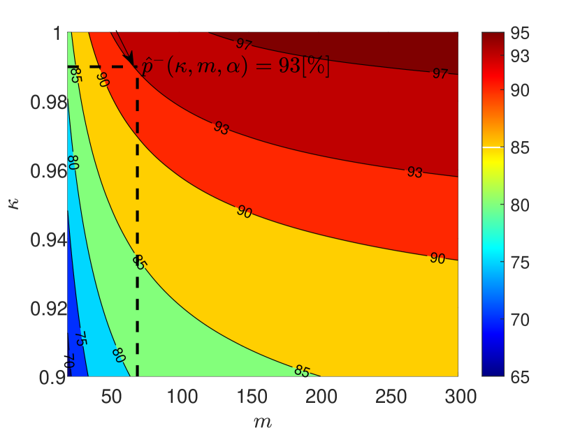
((a))

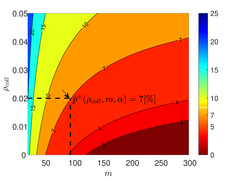
((b))

Figure 4: (4(a)), (4(b)) Values (in percentage) of $\hat{p}^{-}(\kappa,m,\alpha)$ and $\hat{p}^{+}(\rho_{\text{coll}},m,\alpha)$ for $\alpha=0.05$ as a function of the number of MC samples $m$ ($x$-axis) and the coverage approximation factors $\kappa$ and $\rho_{\text{coll}}$ ($y$-axis), respectively.

VI Illustrative Scenario

In this section, we demonstrate the performance of IRIS-U² in a toy scenario using a simple motion model. We start (Sec. VI-A) by describing the setting and continue to describe the methods we will be comparing IRIS-U² with (Sec. VI-B). We finish with a discussion of the results and their implications (Sec. VI-C). Implementation details and code repositories are described in Appendix B.

VI-A Setting

Here we consider the toy scenario depicted in Fig. 5(a) in which we have a two-dimensional workspace that contains $10$ obstacles (red rectangles) and $27$ POIs (red points in seven groups of three). The robot is described by three degrees of freedom—its location $(x,y)$ and heading $\psi$. We model its sensor as having a field-of-view of $94^{\circ}$ and a range of $10[m]$.

We choose a roadmap $\mathcal{G}$ with $27$ vertices (where vertex $0$ is the initial vertex) such that the configuration associated with every vertex is facing up towards the POIs. We note that in the toy scenario, we hand-pick the roadmap only for illustrative purposes, and in practical settings the roadmap would be generated by the systematic approach of IRIS (as in the following section). In the roadmap $\mathcal{G}$, from vertices $0,9$ and $18$, the first three POIs can be seen. Similarly, from vertices $1,10$ and $19$, the next three POIs can be seen, and so on.

Finally, we assume that the environment contains two types of regions corresponding to different levels of uncertainty (to be explained shortly): one (pink, containing vertices $0-9$) with a standard deviation of $\sigma=3[m]$ and the other (light blue, containing vertices $9-26$) with $\sigma=1[m]$.

The motion model we use here, denoted as $\mathcal{M}_{\text{simple}}$, is an extension of $\mathcal{M}_{\text{toy}}$ where parameters $\mathcal{N}_{\rm unc}:=(r,\theta)$ are drawn from the distribution $\mathcal{D}_{\rm unc}$ such that $r=|\mathcal{N}(0,1)|$ if the robot is located in low (pink) uncertainty region and $r=|\mathcal{N}(0,3)|$ if the robot is located in high (light blue) uncertainty region and $\theta=\mathcal{N}(0,2\pi)$. Just as in $\mathcal{M}_{\text{toy}}$, given a command path $\pi^{c}$ with $n>1$ configurations $\pi^{c}=\{\langle x_{1}^{c},y_{1}^{c}\rangle,\ldots\langle x_{n}^{c},y_{n}^{c}\rangle\}$, the corresponding executed path is $\pi_{e}=\{\langle x_{1}^{e},y_{1}^{e}\rangle,\ldots\langle x_{n}^{e},y_{n}^{e}\rangle\}$ such that $x_{i}^{e}=x_{i}^{c}+r\cdot\cos\theta$ and $y_{i}^{e}=y_{i}^{c}+r\cdot\sin\theta$ for $i>1$.

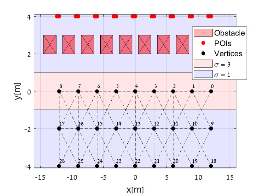
((a))

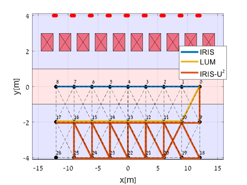
((b))

Figure 5: (5(a)) Illustrative scenario for empirical evaluation. (5(b)) Command paths are computed by IRIS (blue), UP-IRIS (yellow), and IRIS-U² (orange) with $m=100$.

VI-B Baselines

We consider two baselines—the original IRIS algorithm and a straw-man approach which we call uncertainty-penalizing IRIS (UP-IRIS). In UP-IRIS, the cost of an edge is its length added to a penalty factor which is proportional to the uncertainty associated with the edge. As the original IRIS minimizes path length, this modification will compute paths that are both short and have low uncertainty.

We compare the algorithms by obtaining a command-path $\pi^{c}$ from each algorithm and comparing their performance in the execution phase. In preparation for the results, we highlight the distinction between MC samples used in planning and in execution. Planning MC samples are used by IRIS-U² to compute the command-path (referred to as $m$). In contrast, execution MC samples do not affect the command-path and are only used to evaluate the performance of the executed path and IRIS-U²’s CI boundaries.

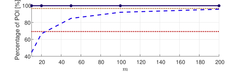
((a))

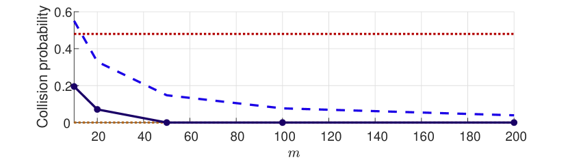
((b))

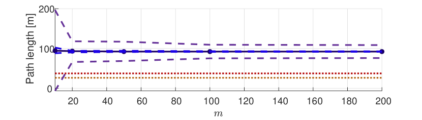
((c))

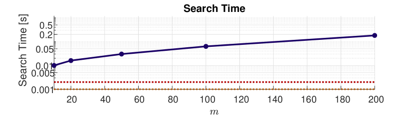
((d))

Figure 6: (6(a))-(6(d)) POI coverage, collision probability, path length, and search time as a function of $m$ for IRIS-U² (blue line) both with the baseline performance of IRIS (red dotted line) and UP-IRIS (orange dotted line) for the toy scenario. Each of figures (6(a))-(6(c)) displays the average of $10,000$ MC execution samples, with the corresponding CI of the expected performance as detailed in Lemma. V.1, V.2, and V.3. In addition, Figure (6(c)) also displays the CI for the sigma level with $n=3$ as detailed in Lemma. V.5.

VI-C Results

To compare IRIS-U² with our baseline, IRIS and UP-IRIS, we ran the planning phase with $\varepsilon=3$ and $\kappa=0.99$. As expected, IRIS (without accounting for uncertainty) computed a command path which is the straight line connecting vertices $0$ and $9$ (blue path in Fig. 5(b)) as it is the shortest path that results in full coverage (when ignoring uncertainty). UP-IRIS on the toy scenario computes a command path (depicted as the yellow path in Fig. 5(b)) which prioritizes regions with low localization uncertainty. This path moves towards vertex $10$ and then proceeding in a straight line towards vertex $17$ while staying within the low-uncertainty region. Similarly, the command path computed by IRIS-U² (represented by the red path in Fig. 5(b)) also prioritizes regions with low localization uncertainty, even though this is not its explicit objective. However, instead of simply traversing through the low-uncertainty region once, IRIS-U² revisits multiple vertices to ensure full coverage.

Numerical results concerning these command paths in the execution phase are depicted in Fig. 6. IRIS achieved an average coverage of $69\%$, significantly lower than the $96\%$ coverage achieved by UP-IRIS. Additionally, the collision probability of IRIS’s path was found to be $47\%$ as opposed to the collision-free execution path of UP-IRIS, as shown in Fig. 6(a) and 6(b).

When looking at the performance of IRIS-U² as a function of $m$, one can see (as to be expected) that the expected POI covered increases up to $99\%$ and that the collision probability decreases down to $0\%$ as $m$ increases (Fig. 6(a) and 6(b), respectively). This comes at the price of longer paths and longer computation times (Fig. 6(c) and 6(d), respectively).

Noteworthy is that in all cases, the CI bounds hold empirically. This is important as our analysis relies on the fact that the probability of inspecting each POI is independent of other POIs (Assumption 1) which may not necessarily hold.

VII Bridge Scenario

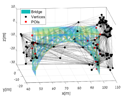
Figure 7: Bridge scenario with $17$ POIs (marked in red). Search is performed on a roadmap $\mathcal{G}$ (marked in black).

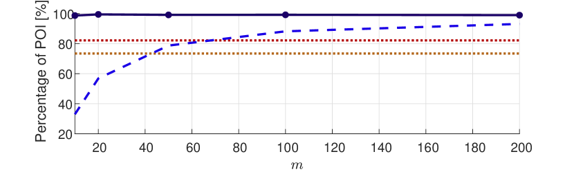
((a))

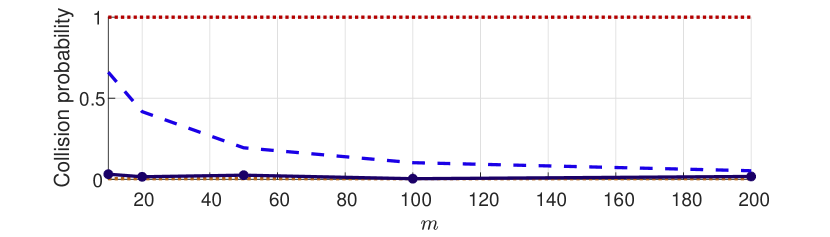
((b))

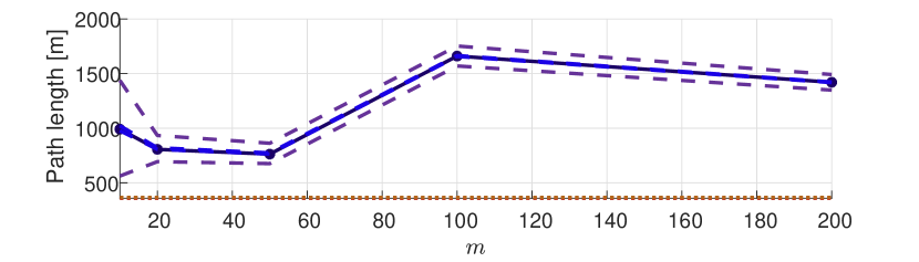
((c))

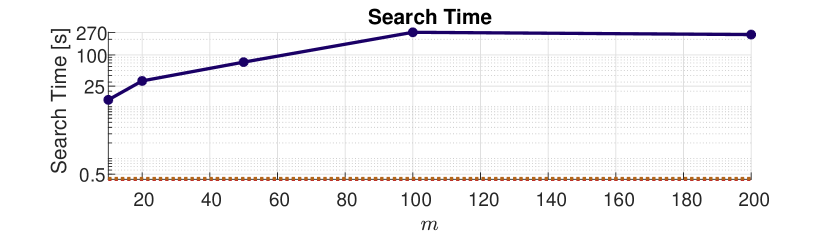
((d))

Figure 8: (8(a))-(8(d)) POI coverage, collision probability, path length, and planning search time as a function of $m$ for IRIS-U² (blue line) both with the baseline performance of IRIS (red dotted line) and UP-IRIS (orange dotted line) for the bridge scenario with $\mathcal{M}_{\text{simple}}$. Each of figures (8(a))-(8(c)) displays the average of $10\,000$ MC execution samples (blue dots), corresponding to the CI of the expected performance (red line) as detailed in Lemma. V.1, V.2, and V.3. In addition, Figure (8(c)) also displays the CI for the sigma level (blue line) with $n=3$ as detailed in Lemma. V.5.

VII-A Motivation and setting

Recall that a key motivation for our work is autonomous bridge inspection [38]. To this end, we consider a UAV with six degrees of freedom corresponding to its location $(x,y,z)\in\mathbb{R}^{3}$ and its orientation $(\phi,\theta,\psi)\in\mathbb{R}^{3}$. We model the sensor as having a field-of-view of $94^{\circ}$ and a range of $10m$. We use the 3D model of a bridge as depicted in Fig. 7 and set the values $\varepsilon=3$ and $\kappa=0.99$. Finally, following [25] the roadmap $\mathcal{G}$ was generated using an RRG [34] with $100$ vertices.

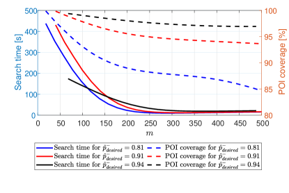
Figure 9: Search time in the planning phase (left $y$-axis) and POI coverage in the execution phase (right $y$-axis) in the bridge scenario using the simple motion model as a function of $m$ for several values of $\hat{p}^{-}_{\text{desired}}$. Here, for each value of $m$, $\kappa$ is the smallest value for which $\hat{p}^{-}(\kappa,m,\alpha)\geq\hat{p}^{-}_{\text{desired}}$ (see Fig. 4).

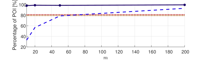
((a))

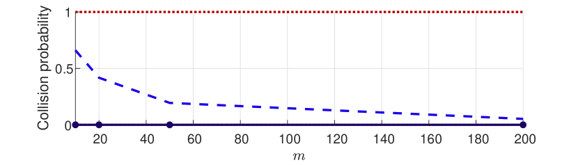
((b))

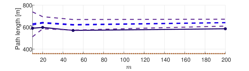
((c))

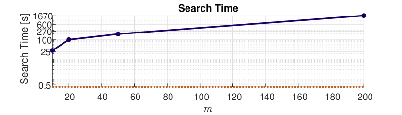
((d))

Figure 10: (10(a))-(10(d)) POI coverage, collision probability, path length, and search time as a function of $m$ for IRIS-U² (blue line) both with the baseline performance of IRIS (red dotted line) and UP-IRIS (orange dotted line) for the bridge scenario with $\hat{\mathcal{M}}_{\text{Simple-GNSS-INS}}$ for the planning and $\mathcal{M}_{\text{full}}$ for the execution. Each of figures (10(a))-(10(c)) displays the average of $100$ MC execution samples (blue dots), corresponding to the CI of the expected performance (red line) as detailed in Lemma. V.1, V.2, and V.3. In addition, Figure (10(c)) also displays the CI for the sigma level (blue line) with $n=3$ as detailed in Lemma. V.5.

VII-B Incorporating the full motion model

We extend the simple motion model $\mathcal{M}_{\text{simple}}$ described in Section VI-A to the 3D setting. Namely, now we sample normally in a sphere around the given location. Specifically, the position error of a specific configuration $(x_{i},y_{i},z_{i},\phi_{i},\theta_{i},\psi_{i})\in\mathbb{R}^{6}$ is given by $d_{x_{i}}=r\cdot\cos\theta\cos\psi$, $d_{y_{i}}=r\cdot\cos\theta\sin\psi$, and $d_{z_{i}}=-r\sin\theta$, where $r\sim|\mathcal{N}(0,\sigma)|$, $\theta\sim\mathcal{N}(0,2\pi)$, and $\psi=\mathcal{N}(0,2\pi)$, where the value $\sigma$ is location dependent. The location uncertainty of an execution path, ${\langle x_{1}^{e},y_{1}^{e},z_{1}^{e}\rangle;\langle x_{2}^{e},y_{2}^{e},z_{1}^{e}\rangle;\ldots}$, when following the command path, ${\langle x_{1}^{c},y_{1}^{c},z_{1}^{c}\rangle;\langle x_{2}^{c},y_{2}^{c},z_{2}^{c}\rangle;\ldots}$, is defined such that (i) $x_{i}^{e}=x_{i}^{c}+d_{x_{i}}$, (ii) $y_{i}^{e}=y_{i}^{c}+d_{y_{i}}$, and (iii) $z_{i}^{e}=z_{i}^{c}+d_{z_{i}}$. We set $\sigma$ to be either $1$ or $3$ corresponding to low and high uncertainty regions, respectively. Specifically, the high uncertainty region is motivated by GNSS outages which typically occur under bridges.

The numerical results concerning these command paths in the execution phase are depicted in Fig. 8. IRIS achieved an average coverage of $82\%$, again, significantly lower than the $98.5\%$ coverage achieved by IRIS-U² even when using only $m=10$. Additionally, the path computed by IRIS was found to be in collision in all cases as opposed to IRIS-U² whose path was found to be collision-free in all tested execution paths.

In the case of UP-IRIS, despite its shorter calculation time and the production of a command path with a low collision probability, it achieved an average coverage of only $73\%$. This highlights the critical significance of considering uncertainty not only in terms of localization uncertainty, which impacts collision probability and path length but also in projecting its effects on the primary objective of inspecting the POIs.

Not surprisingly, to obtain better execution coverage and fewer collisions, IRIS-U² requires longer planning times (see Fig. 8(d)). However, as described in Sec. V-B, for a desired confidence level, we can choose between several parameters. We plot in Fig. 9 the search time for different values of $\kappa$ and $m$. Roughly speaking, increasing $m$ (and thus decreasing $\kappa$) reduces computation time. This is because higher values of $\kappa$ do not allow IRIS-U² to subsume nodes and the computational price of maintaining more nodes is typically larger than using more MC samples. However, after a certain number of MC samples is reached, this trend is reversed. This trade-off is dramatic, for example, when considering a desired value of $\hat{p}^{-}=0.81$ (i.e., at least $81\%$ POIs will be covered for a CL of $1-\alpha=0.95$), the planning times range from $437$ seconds for $\langle m,\kappa\rangle=\langle 18,0.999\rangle$ to $7$ seconds for $\langle m,\kappa\rangle=\langle 200,0.868\rangle$.

VII-C Planning with a simplified motion model

In Sec. VII-B we used a simple motion model both for the planning and the execution phases. A more realistic model (detailed in Appendix B) requires fusing measurements from the GNSS and inertial navigation system (INS) via an EKF, known as inertial navigation system GNSS-INS fusion. Unfortunately, planning with this model yields computation times that are an order of magnitude larger than the already long planning times of IRIS-U². For instance, when comparing the computation time of a single execution path using the full motion model with that of the simplified model, we observed that the former takes approximately $700$ times longer than the latter for the same command path.

To this end, we now demonstrate how IRIS-U² can use a simplified motion model during planning while the full model is only used during execution to evaluate performance. Specifically, in our motion model $\hat{\mathcal{M}}_{\text{Simple-GNSS-INS}}$, we assume that the GNSS-INS system can achieve the same level of accuracy as in the simple motion model described in Sec. VII-B. Underneath the bridge, where GNSS signal reception is typically compromised, the uncertainty accumulates over time. For this region, we adopt a simplified motion model where the robot moves at a constant speed in a straight line between nodes. Following [28], The location uncertainty of an execution path, ${\langle x_{1}^{e},y_{1}^{e},z_{1}^{e}\rangle;\langle x_{2}^{e},y_{2}^{e},z_{1}^{e}\rangle;\ldots}$, when following the command path, ${\langle x_{1}^{c},y_{1}^{c},z_{1}^{c}\rangle;\langle x_{2}^{c},y_{2}^{c},z_{2}^{c}\rangle;\ldots}$, can be expressed as follows:

$$[x_{i}^{e},y_{i}^{e},z_{i}^{e}]=[x_{i}^{c},y_{i}^{c},z_{i}^{c}]+\frac{1}{2}\bm{C_{b_{i}}}\mathbf{b_{a}}t^{2}+\frac{1}{6}\bm{C_{b_{i}}}(\mathbf{b_{g}}\times\mathbf{g})t^{3}.$$ (35)

Here, $\mathbf{g}=\left(0,0,-g\right)$ is the gravity vector, $\mathbf{b_{a}}$ and  $\mathbf{b_{g}}$ are the accelerometer and gyro biases. In addition, ${C_{b_{i}}}$ is the rotation matrix that transforms from the body frame $b$ to the inertial frame $i$, and $t$ is the continuous time spent in the GNSS outages region.

Note that as we use a different execution model from the one used when planning, CI bounds do not necessarily hold. The CI bound of IRIS-U² in this scenario may not accurately reflect the true uncertainty during the execution phase. Indeed, as depicted in Fig. 10, this results in disparities between the executed path length and the CI bounds of IRIS-U². However, despite using a simplified model, IRIS-U² is effective in achieving high execution coverage, with CI bounds that appropriately encapsulate this coverage.

Furthermore, search time is longer here than for the simple motion model as the position error in GNSS outages in this setting is accumulated over time. As a result, the performance (i.e., coverage, collision, and path length) at each vertex in these regions depends on the path history and requires more complex updates. However, we can use the same approach of reducing the search time by using the guidelines described in Sec. V-B. We plot in Fig. 11 the search time for different values of $\kappa$ and $m$ and see similar trends to the results described in Sec. VII-B. Specifically, by accurately balancing $m$ and $\kappa$, we can obtain a speedup of up to $\times 4$ and get a path whose coverage is still above $\hat{p}_{\text{desired}}^{-}$.

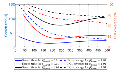
Figure 11: Search time in the planning phase (left $y$-axis) and POI coverage in the execution phase (right $y$-axis) in the bridge scenario using the simplified motion model as a function of $m$ for several values of $\hat{p}^{-}_{\text{desired}}$. Here, for each value of $m$, $\kappa$ is the smallest value for which $\hat{p}^{-}(\kappa,m,\alpha)\geq\hat{p}^{-}_{\text{desired}}$ (see Fig. 4).

We summarize this section with a high-level comparison of the different approaches, also visualized in the accompanying video. As IRIS does not account for uncertainty, the executed path tends to miss POIs and may even collide with the bridge. UP-IRIS, on the other hand, prioritizes low-uncertainty regions and hence typically yields a collision-free executed path, albeit it can still miss POIs. Finally, the planned path of IRIS-U² is typically longer, often traversing edges several times to ensure that no POIs are missed. This is done while ensuring that the path is collision free, even in regions with high uncertainty.

VIII Conclusion and future work

In this study, we proposed IRIS-U², an extension of the IRIS offline path-planning algorithm that considers execution uncertainty through the use of MC sampling. Our empirical results demonstrate that IRIS-U² provides better performance under uncertainty in terms of coverage and collision while providing statistical guarantees via confidence intervals. In addition, we provide a guideline on how to choose parameters to reduce the computation time based on the statistical guarantees.

However, as we discussed in Sec. V-B, the guarantees on the execution path could be affected by a false-negative bias, particularly when there are multiple optional paths in the planning process. As a promising direction, we suggest to explore the Bonferroni correction method [37], and combine it with the information about the number of optional paths considered during planning. By doing so, we can strengthen our CI bounds and enhance the robustness and reliability of our guarantees.

Additionally, recall that we made two key assumptions in this work: (i) that inspecting different POIs is i.i.d (Assumption 1) and (ii) that we wish to minimize path length and not energy consumption or mission completion time (see note following Prob. 1). In future work, we plan to relax both assumptions.

Another direction for future research involves exploring alternative methods to decrease search time. One promising approach is to reduce the number of MC samples by implementing alternative sampling methods such as Latin hypercube sampling (LHS) [39], which better distributes samples across the parameter space. The number of samples can be further reduced by leveraging information from the covariance matrix of the EKF (see, e.g., [8]), particularly when navigation sensors uniformly cover the entire uncertainty region.

Appendix A Statistical Background

In this paper we use CI to evaluate two different types of quantities with respect to the behavior of the IRIS-U² algorithm. The first type is the probability of success for some event, such as the collision probability of a given path being above a certain value. The second type is the mean of a population, such as the expectation of a path’s length. Calculating the CI for these two quantities is done differently and we now detail each method:

Probability of success

To calculate the CI of the success probability of a random variable, we use the Clopper-Pearson method [36]. This method evaluates the maximum likelihood of the probability and its CI assuming a binomial distribution given finite independent trials. Specifically, let $X$ be a random variable whose true unknown probability of success is $\bar{p}$. Let $x_{1},\ldots,x_{m}$ be the outcome of $m$ samples drawn from $X$ (i.e., $x_{i}\in\{0,1\}$) and let $\hat{p}:=\frac{1}{m}\sum_{i=1}^{i=m}{x_{i}}$ be the estimated success probability. Then, according to the Clopper-Pearson method for any $\alpha\in[0,1]$, we can say with CL of $1-\alpha$ that $\bar{p}$, the true unknown success probability of $X$, is within the following the CI:

$$\bar{p}\in\left[\hat{p}^{-}(\hat{p},m,\alpha),\hat{p}^{+}(\hat{p},m,\alpha)\right],$$ (36)

where,

$$\hat{p}^{-}(\hat{p},m,\alpha) :=\frac{\hat{p}\cdot F^{-1}\left(2\hat{p},2\lambda^{-}_{\hat{p},m},1-\frac{\alpha}{2}\right)}{\lambda^{-}_{\hat{p},m}+\hat{p}\cdot F^{-1}\left(2\hat{p},2\lambda^{-}_{\hat{p},m},1-\frac{\alpha}{2}\right)},$$ (37a)

$$\hat{p}^{+}(\hat{p},m,\alpha) :=\frac{\hat{p}^{\prime}\cdot F^{-1}\left(2\hat{p}^{\prime},2\lambda^{+}_{\hat{p},m},\frac{\alpha}{2}\right)}{\lambda^{+}_{\hat{p},m}+\hat{p}^{\prime}\cdot F^{-1}\left(2\hat{p}^{\prime},2\lambda^{+}_{\hat{p},m},\frac{\alpha}{2}\right)}.$$ (37b)

Here, $F^{-1}$ is the inverse F-distribution function [40], $\lambda^{-}_{\hat{p},m}:=m-\hat{p}+1~{}$, $\lambda^{+}_{\hat{p},m}:=m-\hat{p}~{}$ and $\hat{p}^{\prime}:=\hat{p}+1$.

Mean of a population

To calculate the CI of the mean of a population, we follow Habtzghi et al. [36]. Specifically, let $X$ be some random process with unknown mean value $\bar{X}$. In addition, let $x_{1},\ldots,x_{m}$ be $m$ be samples drawn from $X$ and let $\hat{X}:=\frac{1}{m}\sum_{i=1}^{i=m}{x_{i}}$ and $\hat{s}:=\sqrt{\frac{1}{m-1}\sum_{i=1}^{i=m}{\left(x_{i}-\hat{x}\right)^{2}}}$ be their estimated mean and standard deviation, respectively. Then, for any $\alpha\in[0,1]$ we can say with CL of $1-\alpha$ that $\bar{X}$, the true unknown mean value of $X$, is within the following CI:

$$\bar{X}\in\left[\bar{X}^{-}(\hat{X},m,\alpha),\bar{X}^{+}(\hat{X},m,\alpha)\right].$$ (38)

Where,

$$\bar{X}^{-}(\hat{X},m,\alpha):=\hat{X}-t^{*}\frac{\hat{s}}{\sqrt{m}},$$ (39a)

$$\bar{X}^{+}(\hat{X},m,\alpha):=\hat{X}+t^{*}\frac{\hat{s}}{\sqrt{m}}.$$ (39b)

Here, $t^{*}$ is computed according to standard t-tables [41].

It can be useful to bound not only the mean of the population but also its standard deviation. Specifically, following Sheskin et al. [42] for any $\alpha\in[0,1]$ we can say with CL of $1-\alpha$ that $\bar{s}^{2}$, the squared standard deviation of $X$, is within the following CI:

$$\bar{s}^{2}\in\left[\bar{s}^{-}(\hat{s},m,\alpha),\bar{s}^{+}(\hat{s},m,\alpha)\right],$$ (40)

where

$$\bar{s}^{-}(\hat{s},m,\alpha)=\sqrt{\frac{(m-1)\hat{s}^{2}}{\chi^{2}(1-\frac{\alpha}{2})}},$$ (41a)

$$\bar{s}^{+}(\hat{s},m,\alpha)=\sqrt{\frac{(m-1)\hat{s}^{2}}{\chi^{2}(\frac{\alpha}{2})}}.$$ (41b)

Here, $\chi$ is the chi-square distribution [40] and $\hat{s}$ is the estimated standard deviation.

Now, we can use the notion of sigma levels to provide some so-called safety probability that $X$ will not exceed a certain range [43]. Specifically, the sigma level is expressed as a multiple of the standard deviation and is used to determine how many standard deviations a process deviates from its mean, or average, and indicate the degree to which a process is producing results within specifications. Following Shimoyama et al. [43], given a sigma level $n_{l}$, we have a probability $p_{\text{sig lvl}}(n_{l})$ that any possible value of $X$ will be within the following CI:

$$\left[\mu-n\sigma,\mu+n\sigma\right]$$ (42)

where $\mu$ and $\sigma$ are the true unknown mean and standard deviation of $X$, respectively. The number $n_{l}$ is the sigma level (i.e., number of standard deviations) and $p_{\text{sig lvl}}(n_{l})$ is a probability that provided in [43]. For example, $p_{\text{sig lvl}}(1)=68.25\%,p_{\text{sig lvl}}(2)=95.46\%,p_{\text{sig lvl}}(3)=99.73\%$. Thus, we can estimate $\mu$ and $\sigma$ (using Eq. (38) and (40), using the bound value of Eq. (39) and (41) say with CL of $1-\alpha$ that we have a probability $p_{\text{sig lvl}}(n_{l})$ that any possible value of $X$ will be within the following CI:

$$\begin{split}[&\bar{X}^{-}(\hat{X},m,\alpha)-n\bar{s}^{+}(\hat{s},m,\alpha),\\ &\bar{X}^{+}(\hat{X},m,\alpha)+n\bar{s}^{+}(\hat{s},m,\alpha)].\end{split}$$ (43)

Appendix B Code resources

All tests were run on an Intel(R) Core(TM) i7-4510U CPU @ 2.00GHz with 12GB of RAM. The implementation IRIS-U² algorithm is available at https://github.com/CRL-Technion/IRIS-UU.git. We based our implementation of the UAV simulator on the ardupilot model whose implementation can be found at https://wilselby.com/research/arducopter/. This model was extended by incorporating an EKF [28]. The updated version of the UAV simulator, incorporating the EKF, is available at https://github.com/CRL-Technion/Simulator-IRIS-UU.git.

Appendix C Proofs

We provide proofs for our lemmas.

Proof of Lemma V.1: We treat the executed path’s coverage probability as a random variable and recall that $\hat{p}_{j}^{\pi}$ is the estimated probability to inspect POI $j$ computed by $m$ independent samples of execution paths. Then, for any desired CL of $1-\alpha$, the lower bound on the coverage is defined as $\hat{p}{{}_{j}^{\pi}}^{-}=\hat{p}^{-}(\hat{p}_{j}^{\pi},m,\alpha)$. Here, the function $\hat{p}^{-}$ is defined in Eq. (37). Since we assume that the inspection of each POI is independent of the inspection outcomes of the other POIs (see Assumption. 1), we can add up the lower bounds of the individual POIs to obtain a lower bound on the executed path’s coverage. Namely, we can say with a CL of at least $1-\alpha$, a lower bound on the executed path’s coverage is:

$$|\bar{\mathcal{S}}(\pi)|^{-}:=\sum_{j=1}^{j=k}\hat{p}{{}_{j}^{\pi}}^{-}=\sum_{j=1}^{j=k}(\hat{p}_{j}^{\pi},m,\alpha).$$ (44)

$\blacksquare$

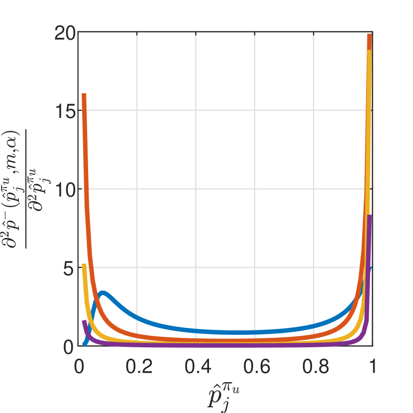
((a)) $\alpha=0.1$

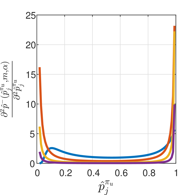
((b)) $\alpha=0.05$

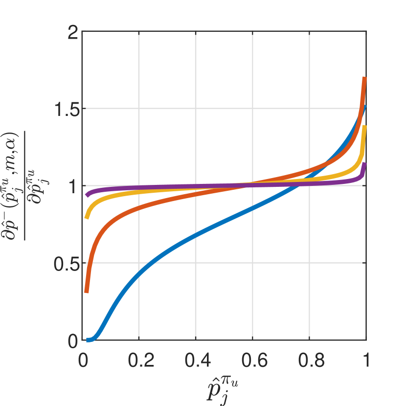
((c)) $\alpha=0.1$

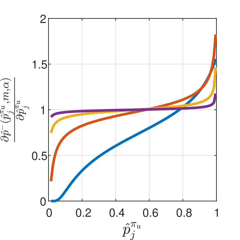
((d)) $\alpha=0.05$

Figure 12: Numerical demonstration that Eq. (49) (12(a) and 12(b)) and Eq. (50) (12(c) and 12(d)) hold for different values of $\alpha$ and $m$.

We now proceed to address the next four lemmas, whose proofs are straightforward. For Lemma V.2, note that since we can treat the executed path’s collision probability as a random variable, Eq. (30) is an immediate application of the Clopper-Pearson method (see Eq. (37)). Similarly, for Lemma V.3 we treat the executed path’s expected length as random variable and Eq. (31) follows from Eq. (38). For Lemma V.4, Eq. (32) is an immediate application of Eq. (40). Finally, for Lemma V.5, Eq. (33) immediately follows from Eq. (43). We proceed to the final proof.

Proof of Lemma V.6: Considering that both values $m$ and $\alpha$ are fixed, it would be convenient to define:

$$f(x):=\hat{p}^{-}(x,m,\alpha).$$ (45)

Assume that minimization of $\sum_{j=1}^{j=k}f(x_{j})$ is achieved for some values $x_{1}^{*},\ldots,x_{k}^{*}$ where $x_{j}^{*}\in[0,1]$ and $\sum_{j=1}^{j=k}x_{j}^{*}\geq k\cdot\kappa$. We need to show that $\forall j,x_{j}^{*}=\kappa$. Finally, recall that $\kappa\in[0,1]$. Thus, we distinguish between the cases where $\kappa=1$ and $\kappa<1$.

Case 1 ($\kappa=1$): Here, $\sum_{j=1}^{j=k}x_{j}^{*}\geq k\cdot\kappa=k$. As $x_{j}^{*}\in[0,1]$, it follows that $\forall j,x_{j}^{*}=1$.

Case 2 ($\kappa<1$): In this case, the proof will be done in two steps: In step 1, we show that minimization of $\sum_{j=1}^{j=k}f(x_{j})$ is achieved when all values of $x_{j}^{*}$ are equal. Namely, $\exists\kappa^{\prime}\geq\kappa$ s.t. $\forall j,x_{j}^{*}=\kappa^{\prime}$. In step 2, we show that this value is obtained for $\kappa^{\prime}=\kappa$ These steps require that Assumption 2 holds. Namely, that $f(x)$ is convex and monotonically increasing.

Case 2, step 1: Let $\kappa^{\prime}\in[\kappa,1)$ be a constant such that $\sum_{j=1}^{j=k}x_{j}^{*}=k\cdot\kappa^{\prime}$ (note that such $\kappa^{\prime}$ always exists). We will prove by contradiction that $\forall j,x_{j}^{*}=\kappa^{\prime}$ which concludes this step.

W.l.o.g., $x_{1}^{*}>\kappa$, i.e., there exists $\delta_{1}>0$ such that $x_{1}^{*}=\kappa+\delta_{1}$. As $\sum_{j=1}^{j=k}x_{j}^{*}=k\cdot\kappa^{\prime}$, there at least one $j\neq 1$ s.t. $x_{j}^{*}<\kappa^{\prime}$. Additionally, w.l.o.g. $x_{2}^{*}<\kappa^{\prime}$. Namely, there exists $\delta_{2}>0$ such that $x_{2}^{*}=\kappa^{\prime}-\delta_{2}$.

Let $\delta=\min(\delta_{1},\delta_{2})$ and consider the following solution $x_{1}^{\prime},\ldots,x_{k}^{\prime}$ to our minimization problem: $x_{1}^{\prime}=x_{1}^{*}-\delta$, $x_{2}^{\prime}=x_{2}^{*}+\delta$ and $x_{j}^{\prime}=x_{j}^{*}$ for $2<j\leq k$. Notice that this is a valid solution (i.e., $\forall j,x_{j}^{\prime}\in[0,1]$ and $\sum_{j=1}^{j=k}x_{j}^{\prime}\geq k\cdot\kappa$). We will show that $\sum_{j=1}^{j=k}f(x_{j}^{\prime})<\sum_{j=1}^{j=k}f(x_{j}^{*})$ which will lead to a contradiction that minimizing $\sum_{j=1}^{j=k}f(x_{j})$ is achieved for $x_{1}^{*},\ldots,x_{k}^{*}$.

As $x_{j}^{\prime}=x_{j}^{*}$ for $2<j\leq k$, to show that $\sum_{j=1}^{j=k}f(x_{j}^{\prime})<\sum_{j=1}^{j=k}f(x_{j}^{*})$, it suffices to prove that:

$$f(x_{1}^{\prime})+f(x_{2}^{\prime})<f(x_{1}^{*})+f(x_{2}^{*}).$$ (46)

This will be done using Assumption 2 (i.e., that $f(\cdot)$ is a strictly convex function). Namely, that $\frac{\partial^{2}f(x)}{\partial^{2}x}>0,\forall x\in[0,1]$ which implies (see, e.g., [44]) that $\forall\lambda$ s.t. $0<\lambda<1$ we have:

$$f(\lambda x_{1}+(1-\lambda)x_{2})<\lambda f(x_{1})+(1-\lambda)f(x_{2}).$$ (47)

Thus,

$$\begin{split}f(x_{1}^{\prime})+f(x_{2}^{\prime})&=f(x_{1}^{*}-\delta)+f(x_{2}^{*}+\delta)\\ &\stackrel{{\scriptstyle(a)}}{{=}}f(x_{1}^{*}-\lambda(x_{1}^{*}-x_{2}^{*}))+f(x_{2}^{*}+\lambda(x_{1}^{*}-x_{2}^{*}))\\ &=f(\lambda x_{2}^{*}+(1-\lambda)x_{1}^{*})+f(\lambda x_{1}^{*}+(1-\lambda)x_{2}^{*})\\ &\stackrel{{\scriptstyle(b)}}{{<}}(1-\lambda)f(x_{1}^{*})+\lambda f(x_{2}^{*})+\\ &~{}~{}~{}~{}\lambda f(x_{1}^{*})+(1-\lambda)f(x_{2}^{*})\\ &=f(x_{1}^{*})+f(x_{2}^{*}).\end{split}$$ (48)

In (a) we use the equation $\lambda=\delta/(x_{1}^{*}-x_{2}^{*})$ and note that $0<\lambda<1$. (b) follows from Eq. (47).

Case 2, step 2: We will prove this step by contradiction. Assume that minimizing $\sum_{j=1}^{j=k}f(x_{j})$ is achieved when $\sum_{j=1}^{j=k}x_{j}^{*}>k\cdot\kappa$. Namely, $\exists\delta>0$ s.t. $\sum_{j=1}^{j=k}x_{j}^{*}=k\cdot(\kappa+\delta)$. Following step 1, $\forall j,x_{j}^{*}=\kappa+\delta$ and $\sum_{j=1}^{j=k}f(x_{j}^{*})=k\cdot f(\kappa+\delta)$.

However, setting $x_{j}^{*}=\kappa$ is also a valid solution for which $\sum_{j=1}^{j=k}f(x_{j}^{*})=k\cdot f(\kappa)$. Following Assumption 2, $f(\cdot)$ is a monotonically increasing function which leads to a contradiction.

$\blacksquare$

As a supplement to the proof of Lemma V.6 we numerically demonstrate that Assumption 2 holds. Specifically, recall that we used $f(x)$ to denote $\hat{p}^{-}(x,m,\alpha)$. Thus, to show that $f(\cdot)$ monotonically increases and is a strictly convex function we wish to show that $\forall\hat{p}_{j}^{\pi_{u}}\in[0,1]$ both:

$$\frac{\partial\hat{p}^{-}(\hat{p}_{j}^{\pi_{u}},m,\alpha)}{\partial\hat{p}_{j}^{\pi_{u}}}>0,$$ (49)

and

$$\frac{\partial^{2}\hat{p}^{-}(\hat{p}_{j}^{\pi_{u}},m,\alpha)}{\partial^{2}\hat{p}_{j}^{\pi_{u}}}>0.$$ (50)

This is demonstrated in Fig. 12 for different values of $m$ and $\alpha$.

Appendix D Illustrative example for possible false negatives

In this section, we present an illustrative example that serves to elucidate the notion of false negatives eluded to in Sec.V. The purpose of this example is to shed light on how the use of statistical guarantees, such as those outlined in Sec.V-A, can potentially lead to erroneous conclusions when applied to the output of the IRIS-U² algorithm under specific conditions.

Specifically, consider a scenario in which IRIS-U² is configured with $\rho_{\rm coll}=0$, meaning that if the algorithm outputs a path $\pi$, it confidently asserts that $\hat{C}(\pi)=0$, indicating that the path is collision-free.

Furthermore, assume that the algorithm uses $m=120$. As established in Lemma V.2, when considering a given path $\pi$ and setting $\alpha=0.05$, we find that $\bar{C}(\pi)^{+}\approx 0.03$. This implies a $95\%$ probability that if this path is executed $100$ times, at most $3$ of these executions will result in collisions.

Now, let’s examine a situation where the false-negative bias comes into play — when there is more than one option for the command path. For instance, assume we have $k=100$ paths, denoted as $\pi_{1},\ldots,\pi_{k}$, connecting the start and the goal where each of these paths has a true collision probability of $\bar{C}(\pi_{i})=0.04$. The probability that a specific path will be estimated to be collision-free is:

$$(1-\bar{C}(\pi_{i}))^{m}=0.96^{120}\approx 0.0075.$$

However, the false-negative bias effect lies in the probability that at least one of the $k$ paths will be estimated as collision-free:

$$1-\left(1-(\bar{C}(\pi_{i}))^{m}\right)^{k}\approx 1-\left(1-0.0075\right)^{100}\approx 0.52.$$

Namely, there is more than $50\%$ chance that the algorithm will output a path $\pi_{i}$ assumed to be collision-free whose true collision probability is $4\%$ (which, of course, is larger than the upper bound of $\bar{C}(\pi_{i})^{+}\approx 0.03$ guaranteed with $95\%$ confidence if Lemma V.2 was wrongly used).

References

- [1] A. Bircher, M. Kamel, K. Alexis, M. Burri, P. Oettershagen, S. Omari, T. Mantel, and R. Siegwart, “Three-dimensional coverage path planning via viewpoint resampling and tour optimization for aerial robots,” Autonomous Robots, vol. 40, no. 6, pp. 1059–1078, 2016.
- [2] B. McGuire, R. Atadero, C. Clevenger, and M. Ozbek, “Bridge information modeling for inspection and evaluation,” Journal of Bridge Engineering, vol. 21, no. 4, p. 04015076, 2016.
- [3] B. Chan, H. Guan, J. Jo, and M. Blumenstein, “Towards UAV-based bridge inspection systems: A review and an application perspective,” Structural Monitoring and Maintenance, vol. 2, no. 3, pp. 283–300, 2015.
- [4] E. Galceran and M. Carreras, “A survey on coverage path planning for robotics,” Robotics and Autonomous systems, vol. 61, no. 12, pp. 1258–1276, 2013.
- [5] T. Danner and L. E. Kavraki, “Randomized planning for short inspection paths,” in Proceedings 2000 ICRA. Millennium Conference. IEEE International Conference on Robotics and Automation. Symposia Proceedings (Cat. No. 00CH37065), vol. 2. IEEE, 2000, pp. 971–976.
- [6] B. Englot and F. Hover, “Inspection planning for sensor coverage of 3d marine structures,” in 2010 IEEE/RSJ International Conference on Intelligent Robots and Systems. IEEE, 2010, pp. 4412–4417.
- [7] B. J. Englot and F. S. Hover, “Sampling-based coverage path planning for inspection of complex structures,” in Twenty-Second International Conference on Automated Planning and Scheduling, 2012.
- [8] C. Papachristos, M. Kamel, M. Popović, S. Khattak, A. Bircher, H. Oleynikova, T. Dang, F. Mascarich, K. Alexis, and R. Siegwart, “Autonomous exploration and inspection path planning for aerial robots using the robot operating system,” in Robot Operating System (ROS). Springer, 2019, pp. 67–111.
- [9] G. Papadopoulos, H. Kurniawati, and N. M. Patrikalakis, “Asymptotically optimal inspection planning using systems with differential constraints,” in 2013 IEEE International Conference on Robotics and Automation. IEEE, 2013, pp. 4126–4133.
- [10] A. Bircher, K. Alexis, U. Schwesinger, S. Omari, M. Burri, and R. Siegwart, “An incremental sampling-based approach to inspection planning: the rapidly exploring random tree of trees,” Robotica, vol. 35, no. 6, pp. 1327–1340, 2017.
- [11] Y. Sun, M. Liu, and M. Q.-H. Meng, “Wifi signal strength-based robot indoor localization,” in 2014 IEEE International Conference on Information and Automation (ICIA). IEEE, 2014, pp. 250–256.
- [12] M. E. Rida, F. Liu, Y. Jadi, A. A. A. Algawhari, and A. Askourih, “Indoor location position based on bluetooth signal strength,” in 2015 2nd International Conference on Information Science and Control Engineering. IEEE, 2015, pp. 769–773.
- [13] L. L. Whitcomb, D. R. Yoerger, H. Singh, and J. Howland, “Combined doppler/lbl based navigation of underwater vehicles,” in Proceedings of the the 11th international symposium on unmanned untethered submersible technology, vol. 9818. Citeseer, 1999.
- [14] N. Haala, M. Peter, J. Kremer, and G. Hunter, “Mobile lidar mapping for 3d point cloud collection in urban areas—a performance test,” Int. Arch. Photogramm. Remote Sens. Spat. Inf. Sci, vol. 37, pp. 1119–1127, 2008.
- [15] I. Klein, S. Filin, and T. Toledo, “Vehicle constraints enhancement for supporting ins navigation in urban environments,” NAVIGATION, Journal of the Institute of Navigation, vol. 58, no. 1, pp. 7–15, 2011.
- [16] R. Pepy and A. Lambert, “Safe path planning in an uncertain-configuration space using rrt,” in 2006 IEEE/RSJ International Conference on Intelligent Robots and Systems. IEEE, 2006, pp. 5376–5381.
- [17] R. Alami and T. Simeon, “Planning robust motion strategies for a mobile robot,” in Proceedings of the 1994 IEEE International Conference on Robotics and Automation. IEEE, 1994, pp. 1312–1318.
- [18] S. Candido and S. Hutchinson, “Minimum uncertainty robot path planning using a pomdp approach,” in 2010 IEEE/RSJ International Conference on Intelligent Robots and Systems. IEEE, 2010, pp. 1408–1413.
- [19] J.-A. Delamer, Y. Watanabe, and C. P. Carvalho Chanel, “Solving path planning problems in urban environments based on a priori sensors availabilities and execution error propagation,” in AIAA Scitech 2019 Forum, 2019, p. 2202.
- [20] B. Englot, T. Shan, S. D. Bopardikar, and A. Speranzon, “Sampling-based min-max uncertainty path planning,” in 2016 IEEE 55th Conference on Decision and Control (CDC). IEEE, 2016, pp. 6863–6870.
- [21] A. Wu, T. Lew, K. Solovey, E. Schmerling, and M. Pavone, “Robust-rrt: Probabilistically-complete motion planning for uncertain nonlinear systems,” in International Foundation of Robotics Research, 2022.
- [22] D. Zheng and P. Tsiotras, “Ibbt: Informed batch belief trees for motion planning under uncertainty,” arXiv preprint arXiv:2304.10984, 2023.
- [23] Q. H. Ho, Z. N. Sunberg, and M. Lahijanian, “Gaussian belief trees for chance constrained asymptotically optimal motion planning,” in International Conference on Robotics and Automation. IEEE, 2022, pp. 11 029–11 035.
- [24] A. R. Pedram, R. Funada, and T. Tanaka, “Gaussian belief space path planning for minimum sensing navigation,” IEEE Trans. Robotics, vol. 39, no. 3, pp. 2040–2059, 2023.
- [25] M. Fu, A. Kuntz, O. Salzman, and R. Alterovitz, “Asymptotically optimal inspection planning via efficient near-optimal search on sampled roadmaps,” Int. J. Robotics Res., vol. 42, no. 4-5, pp. 150–175, 2023.
- [26] A. Hazra, “Using the confidence interval confidently,” Journal of thoracic disease, vol. 9, no. 10, p. 4125, 2017.
- [27] S. Thrun, W. Burgard, and D. Fox, Probabilistic robotics. MIT Press, 2005.
- [28] P. Groves, Principles of GNSS, Inertial, and Multisensor Integrated Navigation Systems, Second Edition, 03 2013.
- [29] J. N. Gross, Y. Gu, and M. B. Rhudy, “Robust uav relative navigation with dgps, ins, and peer-to-peer radio ranging,” IEEE Transactions on Automation Science and Engineering, vol. 12, no. 3, pp. 935–944, 2015.
- [30] M. Khaghani and J. Skaloud, “Autonomous vehicle dynamic model-based navigation for small uavs,” NAVIGATION: Journal of the Institute of Navigation, vol. 63, no. 3, pp. 345–358, 2016.
- [31] S. M. LaValle, Planning Algorithms. Cambridge, U.K.: Cambridge University Press, 2006.
- [32] O. Salzman, “Sampling-based robot motion planning,” Commun. ACM, vol. 62, no. 10, pp. 54–63, 2019.
- [33] P. E. Hart, N. J. Nilsson, and B. Raphael, “A formal basis for the heuristic determination of minimum cost paths,” IEEE Trans. Systems Science and Cybernetics, vol. 4, no. 2, pp. 100–107, 1968.
- [34] S. Karaman and E. Frazzoli, “Sampling-based algorithms for optimal motion planning,” Int. J. Robotics Research, vol. 30, no. 7, pp. 846–894, Jun. 2011.
- [35] J. Neyman, “Outline of a theory of statistical estimation based on the classical theory of probability,” Philosophical Transactions of the Royal Society of London. Series A, Mathematical and Physical Sciences, vol. 236, no. 767, pp. 333–380, 1937.
- [36] D. Habtzghi, C. Midha, and A. Das, “Modified clopper-pearson confidence interval for binomial proportion.” J. Stat. Theory Appl., vol. 13, no. 4, pp. 296–310, 2014.
- [37] E. W. Weisstein, “Bonferroni correction,” https://mathworld. wolfram. com/, 2004.
- [38] J. Wells and B. Lovelace, “Improving the quality of bridge inspections using unmanned aircraft systems (uas),” Tech. Rep., 2018.
- [39] W.-L. Loh, “On latin hypercube sampling,” The annals of statistics, vol. 24, no. 5, pp. 2058–2080, 1996.
- [40] L. Knüsel, “Computation of the chi-square and poisson distribution,” SIAM Journal on Scientific and Statistical Computing, vol. 7, no. 3, pp. 1022–1036, 1986.
- [41] P. A. Games, “An improved t table for simultaneous control on g contrasts,” Journal of the American Statistical Association, vol. 72, no. 359, pp. 531–534, 1977.
- [42] D. J. Sheskin, Handbook of parametric and nonparametric statistical procedures. Chapman and Hall/CRC, 2011.
- [43] K. Shimoyama, A. Oyama, and K. Fujii, “Development of multi-objective six sigma approach for robust design optimization,” Journal of aerospace computing, information, and communication, vol. 5, no. 8, pp. 215–233, 2008.
- [44] M. Grasmair, “Basic properties of convex functions,” Department of Mathematics, Norwegian University of Science and Technology, 2016.