Real time evolution of scalar fields with kernelled Complex Langevin equation

Abstract

The real time evolution of a scalar field in 0+1 dimensions is investigated on a complex time contour. The path integral formulation of the system has a sign problem, which is circumvented using the Complex Langevin equation. Measurement of the boundary terms allow for the detection of correct results (for contours with small real time extents) or incorrect results (at large real time extents), as confirmed by comparison to exact results calculated using diagonalization of the Hamiltonian. We introduce a constant matrix kernel in the Complex Langevin equation, which is optimized with the requirement that distributions of the fields on the complexified manifold remain close to the real manifold. We observe that reachable real times are roughly twice as large with the optimal kernel. We also investigate field dependent kernels represented by a neural network for a toy model as well as for the scalar field, providing promising first results.

I Introduction

Ab initio calculations of real-time quantities in Quantum field theories (QFT) is one of the main challenges of theoretical physics. Non-equilibrium physics of quantum field theories can be tackled using various approximations such as the classical approximation, functional equations and the kinetic approximation, however these approaches have systematic errors which are very hard to control. In contrast, lattice discretisation has relatively easy to control systematics, and has proven to be a very useful tool in studying QFTs. Lattice calculations are usually formulated in imaginary time, leading to a theory suitable for importance sampling Monte Carlo simulations. In contrast, using real-time lattices (e.g. with the aim of investigating non-equilibrium phenomena) leads to a path integral with complex measure $\exp(iS)$ with the (real valued) action $S$, so naive importance sampling simulations are invalidated by the sign-problem. Even some equilibrium quantities are affected by this problem: real-time correlators such as those needed in the Kubo formulas for hydrodynamical transport coefficients, spectral functions of bounded states or parton distribution functions, while in principle accessible starting from the euclidean theory, they require the inversion of an integral kernel, which often leads to an underdetermined system of equations, usually solved with Bayesian methods or with the usage of further assumptions or modeling of the system (see the recent review Rothkopf:2022ctl ). Other problems, such as the tunneling rate between metastable vacua in QFTs or the equilibration of the matter in the initial stages of a heavy ion collision present a non-equilibrium problem inaccessible to euclidean simulations.

The sign problem can be (partially) circumvented in various ways, for a recent reviews of different methods see Berger:2019odf ; Alexandru:2020wrj ; Nagata:2021ugx . In this paper we concentrate on the Complex Langevin equation (CLE)Klauder:1983nn ; Parisi:1984cs , which was proposed to circumvent the sign problem by complexifying the simulation manifold, such that the original theory is recovered in expectation values using analytic continuation of the observables. Among many applications ranging from systems at nonzero density or theta-term to condensed matter models with fermionic imbalance (for a recent review see Berger:2019odf ; Attanasio:2020spv ), the CLE was also used to study Quantum Field theories in Minkowski spacetime Huffel:1984mq ; Callaway:1985vz ; Nakazato:1985zj . The CLE was first applied to investigate non-equilibrium physics in Berges2005b . In Berges:2006xc ; Berges:2007nr a variant of the Schwinger-Keldysh contour was introduced for the lattice discretisation, which allows equilibrium as well as non-equilibrium simulations, and a scalar oscillator and a 3+1 dimensional SU(2) pure gauge theory was investigated.

The problem of real-time simulations has also been tackled by a close relative of the Complex Langevin method: optimized complexified manifolds Alexandru:2016gsd ; Alexandru:2020wrj (as inspired by simulations on Lefschetz-thimbles Cristoforetti:2012su ), observing that similarly to complex Langevin, real time extents with the magnitude of about a period of the oscillator are reachable (for larger time extents the costs of the simulation get too high).

The Langevin equation (as well as the CLE) allows a modification with a kernel Soderberg:1987pd ; Okamoto:1988ru ; Okano:1991tz , which leaves the stationary solution of the corresponding Fokker-Planck equation unchanged. In this paper we introduce a kernel in the Complex Langevin equation such that boundary terms are reduced. We search for an optimal kernel using Machine Learning inspired methods. We first use field independent kernels, afterwards we do the first exploratory steps in finding field dependent kernels. We study an anharmonic quantum oscillator as well as a toy model to help understand the behavior of the kernel optimization process. A study with a similar aim has appeared recently Alvestad:2022abf which was carried out independently from our study. Another recent application of an anisotropic, constant kernel has been studied in real-time simulations of a SU(2) pure gauge theory Boguslavski:2022dee .

The paper is organized as follows: In section II, we introduce the Complex Langevin equation, boundary terms, kernels. Section III is devoted to the anharmonic quantum oscillator: we show results using naive CLE, discuss our optimization procedure for a constant kernel, and show the results of the optimally kernelled CLE. In section IV we discuss field dependent kernels, described with a suitable ansatz as well as with a neural network, as applied to a toy model and the quantum oscillator. Finally in section V we summarize our results and conclude.

II Complex Langevin eq., Kernels and numerical setup

In the path integral formulation, a quantum mechanical system is defined in terms of its path integral with the measure $\exp(iS)$ with the action $S$. For an imaginary time contour the action is imaginary, giving a real and positive measure. For a non-strictly imaginary time-contour the action is in general complex, which leads to the appearance of the sign-problem, invalidating importance sampling Monte Carlo simulations. To circumvent this problem, we use the complex Langevin equation (CLE) Parisi:1984cs ; Klauder:1983nn , which is given by

$${\partial\phi_{i}(\tau)\over\partial\tau}=-{\partial S\over\partial\phi_{i}}+\eta_{i}(\tau),$$ (1)

where we introduced the Langevin time $\tau$, and $i$ indexes the fields on a space-time lattice along some complex-time contour, and $\eta_{i}(\tau)$ is a Gaussian noise term satisfying $\langle\eta_{i}(\tau)\rangle=0,\ \ \langle\eta_{i}(\tau)\eta_{j}(\tau^{\prime})\rangle=2\delta_{ij}\delta(\tau-\tau^{\prime})$.

The complex Langevin equation is known to sometimes produce wrong results due to either insufficient decay of the distribution at infinity or non-holomorphic actions Aarts:2009uq ; Aarts:2011ax ; Aarts:2017vrv ; Seiler:2023kes . These can be characterised by boundary terms, which can be measured using the complexified process only boundaryterms1 ; boundaryterms2 . The boundary terms are given in terms of some norm $N(\phi)$ and a cutoff variable $Y$, such that $N(\phi)<Y$ defines a compact set containing the original real manifold. To extract the boundary terms for some observable $O(\phi)$, one has to measure

$$\lim_{Y\rightarrow\infty}\left\langle\theta(Y-N(\phi))\sum_{i}(\partial_{i}+K_{i})\partial_{i}O(\phi)\right\rangle,$$ (2)

such that a nonzero value signals an incorrect CLE result. (For a more detailed explanation, see boundaryterms1 ; boundaryterms2 ).

Setting up the Langevin equation one has a great amount of freedom. One of the allowed modifications is called a kernel Soderberg:1987pd ; Okamoto:1988ru ; Okano:1991tz . The kernelled Langevin equation for a single degree of freedom reads

$${dz\over d\tau}=-K(z){\partial S\over\partial z}+{\partial K(z)\over\partial z}+\sqrt{2K(z)}\eta(\tau),$$ (3)

where we have defined $K(z)$, the field dependent kernel. For scalar fields $\phi_{i},\ i=1..N$ we write

$${d\phi_{i}\over d\tau}=-H_{ij}(\phi)H^{T}_{jk}(\phi){\nabla_{k}S}+\partial_{k}(H_{ij}(\phi)H^{T}_{jk}(\phi))+H_{ij}(\phi)\eta_{j},$$ (4)

where $\nabla_{i}$ is differentiation with respect to the $i$-th scalar variable and using a field dependent matrix $H_{ij}(\phi)$, which is assumed to be symmetric below. In older literature the square of this matrix $K_{ij}(\phi)=H_{ik}(\phi)H_{kj}(\phi)$ is called the kernel. Such a kernel can be used for e.g. Fourier acceleration of the Langevin simulations Batrouni:1985jn . Using $H_{ij}=\delta_{ij}$ gives back the original Langevin equation. Note that a constant kernel $H_{ij}=C\delta_{ij}$ is just a redefinition of the Langevin time using the scaling $\tau^{\prime}=\sqrt{C}\tau$. It has been shown in Aarts:2012ft that a subclass of kernels is equivalent to setting up the Langevin equation after a variable change in the path integral has taken place. It’s easy to show that a kernel changes the scalar Fokker-Planck equation into

$$\partial_{\tau}P(\phi,\tau)=\nabla_{i}(H_{ik}H_{jk}(\nabla_{j}+\nabla_{j}S))P(\phi,\tau),$$ (5)

where $P(\phi,\tau)$ is the probability distribution of the variables at Langevin time $\tau$. From this one notices that the standard $P=e^{-S}$ remains a stationary solution of the Fokker-Planck operator. The stability properties as well as the uniqueness of this solution might change in general. It is shown below that with a careful choice of the kernel one can improve the stability properties of the equilibrium distribution, and in practice one might use a kernel to reduce boundary terms in the simulation of the Complex Langevin equation.

III Real-time evolution of the anharmonic quantum oscillator

The model we investigate is a scalar field theory with a quartic self-coupling, defined by the action

$$S=\int dtd^{d}x\left({1\over 2}\dot{\phi}^{2}-{1\over 2}(\nabla\phi)^{2}-V(\phi)\right),\quad V(\phi)={1\over 2}m^{2}\phi^{2}+{\lambda\over 24}\phi^{4}.$$ (6)

The path integral describing the quantum mechanical evolution of the system in turn contains the measure $\exp(iS)$. An imaginary temporal path starting at $t=0$ and ending at $t=-i\beta$ allows the description of a thermal state with temperature $T=1/\beta$, when one uses periodical boundary conditions. To study real-time correlators (or in general, real time evolution), we discretise the system on a complex time-contour Berges:2006xc , using $C_{t},\ \ t=0...N$ with $C_{0}=0$ and $\textrm{Re}C_{N}=0$, and the complex time-step $\Delta_{t}=C_{t+1}-C_{t}$. We use periodic boundary conditions $\phi_{0}(x)=\phi_{N}(x)$ such that the system is in thermal equilibrium. The discretised action for a $d+1$ dimensional theory then reads

$$S={1\over 2}\sum_{t,x}\left({(\phi_{t+1}(x)-\phi_{t}(x))^{2}\over\Delta_{t}}-{\Delta_{t}\over 2}\sum_{\nu=1}^{d}\left((\phi_{t}(x+\hat{\nu})-\phi_{t}(x))^{2}+(\phi_{t+1}(x+\hat{\nu})-\phi_{t+1}(x))^{2}\right)-\Delta_{t}\left(V(\phi_{t})+V(\phi_{t+1})\right)\right)$$ (7)

with the field $\phi_{t}(x)=\phi(C_{t},x)$ and $x+\hat{\nu}$ denoting the neighbouring lattice site in spatial direction $\nu$. In the following we consider a 0+1 dimensional system corresponding to an anharmonic quantum oscillator.

We have used a triangle contour on the complex time plane, starting at $t_{\textrm{start}}=0$, following a straight line to the turning point $t_{\textrm{mid}}=t_{\textrm{max}}-0.01i\beta$, and again following a straight line to the endpoint $t_{\textrm{end}}=-i\beta$. (We have checked that our results remain unchanged when using a horizontal upper part of the triangle contour such that $t_{\textrm{mid}}=t_{\textrm{max}}$.) We use periodic boundary conditions such that the path integral describes the oscillator in thermal equilibrium. This temporal path is discretised to $N_{t}/2$ equidistant points on the upper part of the contour and $N_{t}/2$ equidistant points on the lower part. We use the parameters $m^{2}=1,\lambda=24$ and $\beta=1$, and various $t_{\textrm{max}}$ values. An improved update equation as well as adaptive step size are used for all calculations. The maximal Langevin step size is chosen to be $\Delta\tau=10^{-5}$.

Our two main observables are the equal-time two point function $\langle\phi(t)^{2}\rangle$ (which is time independent in thermal equilibrium), and the unequal-time two point function $\langle\phi(0)\phi(t)\rangle$. The exact results for these correlators for a general complex $t$ parameter can be calculated using the truncation of the Hamiltonian operator in particle number basis, and performing the exponentiation of the truncated matrix in its eigenbasis. To get precise results for the purposes of this study, one needs to truncate to about $N=32$ states.

Judging whether the CLE (with or without a kernel) delivers correct results can proceed in various ways. As the system we are studying is in thermal equilibrium, all correlators should be time translation invariant. First, the easiest check is therefore to study an equal-time two point function (The one point function is zero, even if the CLE results are wrong for other observables.), $\langle\phi(t)^{2}\rangle$. Significant deviations from a constant in time mean that boundary terms are non-zero and the results are incorrect. Second, we can explicitly measure boundary terms as discussed above. Third, for this simple model we can calculate the exact results using diagonalization, this is however going to be infeasible for eventual applications of this method for scalar field theories as we study the theory in $d>0$ spatial dimensions.

III.1 Boundary terms

In this subsection we show the results of the naive (un-kernelled) Langevin equation and the boundary terms. In Fig. 1 we show the results for the two point function $\langle\phi(t)^{2}\rangle$ as a function of time for two different time extents. In thermal equilibrium this quantity has to be time independent, therefore one notes that a time dependent CLE result is certainly wrong for the larger real-time extents. This is confirmed by comparing to the exact results gained by diagonalization, as showed on the plot.

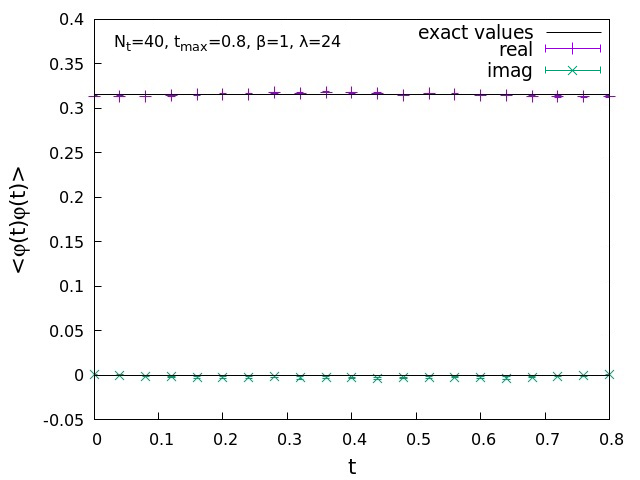
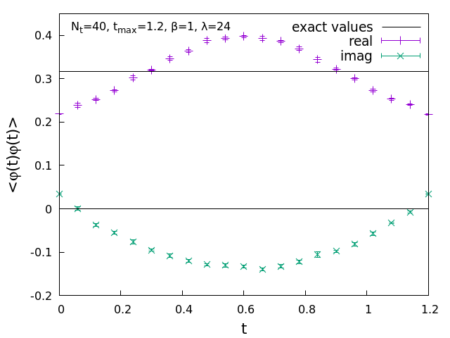
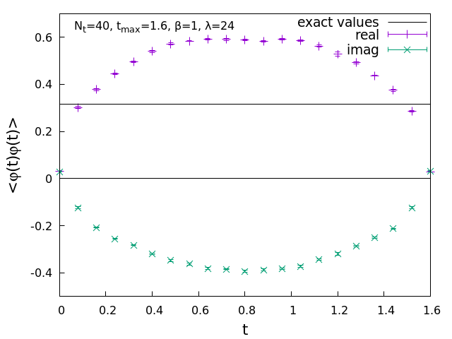
Figure 1: Results for the two point function $\langle\phi(t)^{2}\rangle$ for a real-time extent of 0.8 (left), 1.2 (middle) and a real-time extent of 1.6 (right), calculated with the CLE without a kernel.

In Fig. 2 we show the corresponding boundary terms, and one observes that they nicely signal incorrect results from the CLE dynamics itself, without needing to know the exact results beforehand.

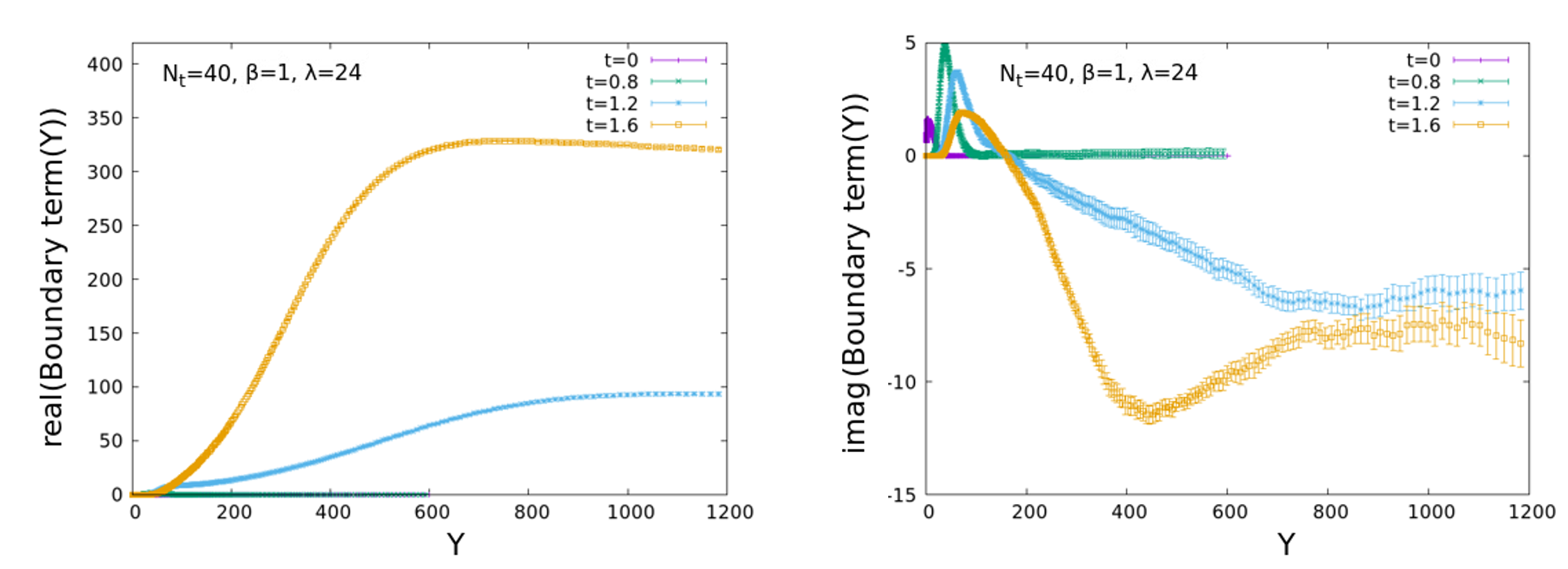
Figure 2: Real part (left) and imaginary part (right) of the boundary terms for the observable $\phi^{2}$ for different real-time extents, as calculated from a simulation with the un-kernelled CLE.

The unequal-time two point function $\langle\phi(0)\phi(t)\rangle$ is shown in Fig. 3, where, similarly to $\langle\phi(t)^{2}\rangle$, the short time extent shows correct results while for the larger time extents discrepancies appear.

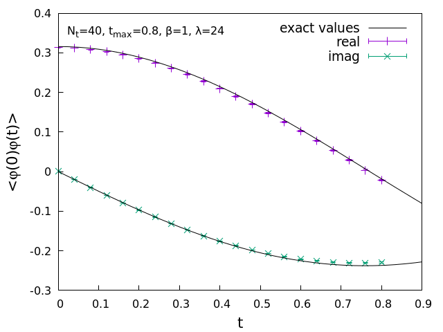
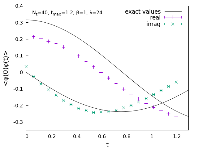
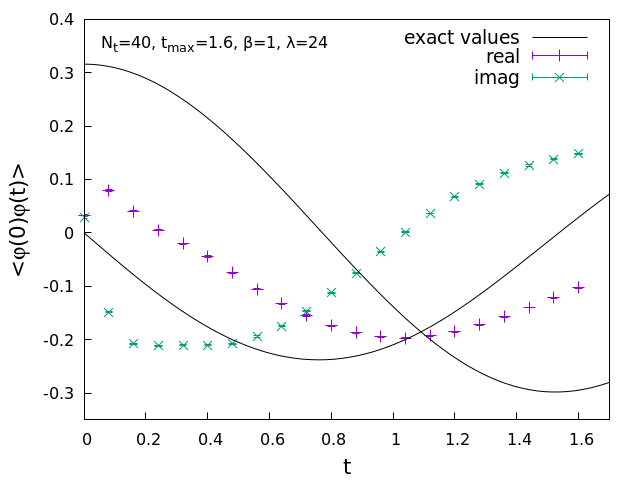
Figure 3: Results for the two point function $\langle\phi(0)\phi(t)\rangle$ for a real-time extent of 0.8 (left), 1.2 (middle) and 1.6 (right), as calculated from a simulation with the un-kernelled CLE.

III.2 Introducing a constant kernel in the CLE

In this subsection we investigate the performance of a constant kernel in the complex Langevin equation for the real-time anharmonic oscillator, such that the CLE is given by

$${d\phi_{i}\over d\tau}=-H_{ij}H^{T}_{jk}{\nabla_{k}S}+H_{ij}\eta_{j},$$ (8)

To find the optimal kernel, we use the stochastic gradient descent method. Our loss function to be minimized is the norm

$$N(\phi)=\sum_{i}F_{1}(\textrm{Re}\,\phi)^{2}+F_{2}(\textrm{Im}\,\phi)^{2},$$ (9)

where we use $F_{1}=0,\ F_{2}=1$ below, if not otherwise noted. The updated field from the CLE reads as

$$\phi_{i}^{\prime}=\phi_{i}-H_{iz}(\phi)H^{T}_{zy}(\phi){\nabla_{y}S}\Delta\tau+H_{iy}(\phi)\eta_{y}\sqrt{\Delta\tau}.$$ (10)

To make the norm minimal after the timestep, we can update our matrix split to real and imaginary parts $H_{ij}=a_{ij}+ib_{ij}$ using

$$a^{\prime}_{ij}=a_{ij}-\Delta L{\partial N(\phi^{\prime})\over a_{ij}},\quad b^{\prime}_{ij}=b_{ij}-\Delta L{\partial N(\phi^{\prime})\over b_{ij}},$$ (11)

where $\Delta L$ is the learning step size. In practice we average the gradient terms using the following procedure: we start out with $H_{ij}=\delta_{ij}$ and set the $\phi_{i}$ fields to zero. We update the Langevin equation with the current kernel, and thermalize for a Langevin time of 100. We then collect all the configurations for a Langevin time interval of 1. Since we use an adaptive step size with a maximal step $\Delta\tau=10^{-5}$, this means at least $10^{5}$ configurations. We use the configurations to calculate and average the gradient terms in eq. (11). We then update $a_{ij}$ and $b_{ij}$ using the averaged gradients. After $10^{6}$ of such learning steps, the fields are again set to 0 (to prevent them from wondering too far) and the process is repeated until the matrix is sufficiently converged. We typically use $\Delta L=10^{-4}-10^{-3}$. To avoid an overall rescaling of the Langevin time, we scale the matrix such that the sum squared of matrix elements is fixed. In Fig. 4 we show a sample of the learning process for some elements of the matrix $H$, for a simulation with real-time extent 1.2 and $N_{t}=20$. One observes that the matrix elements typically equilibrate after $10^{7}$ learning steps.

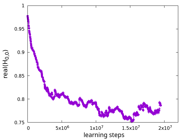
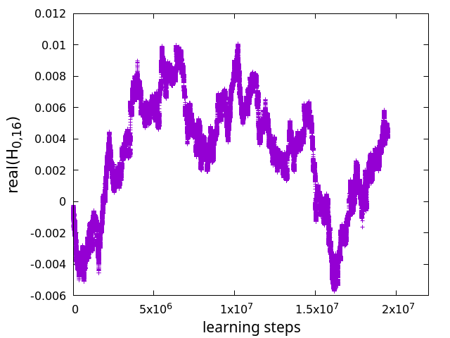
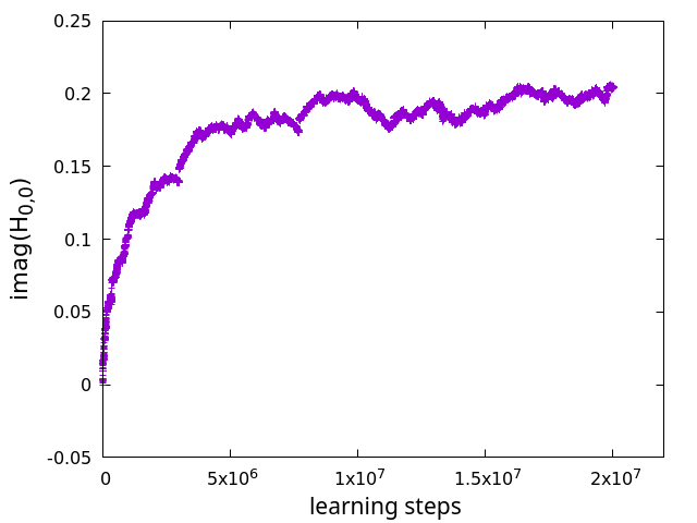
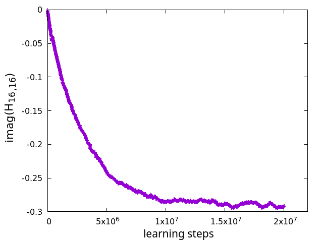
Figure 4: Convergence of different matrix elements of a constant kernel for a real-time extent of 1.2 during the learning process for N=20.

The converged kernels have their largest magnitude elements on the diagonal, with significant contributions also to the first super- and sub-diagonal elements (with periodic boundary conditions). These nearest neighbour ”couplings” have their largest magnitude values near the turning points of the contour. The rest of the matrix elements are small, nonzero values. In Fig. 5 we show the converged kernels for real-time extents $t=1.2$ and $t=2.0$.

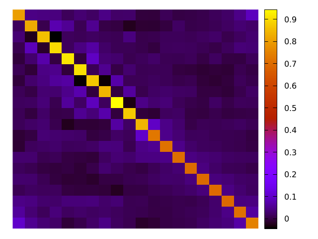
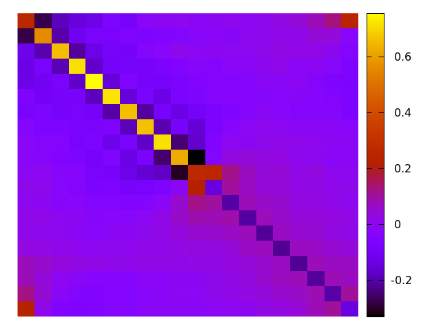
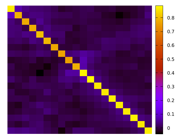
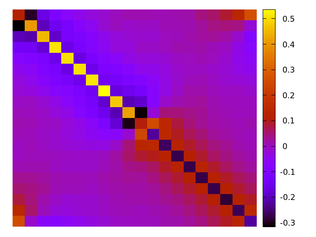
Figure 5: Converged kernel matrices for real-time extents of 1.2 (real part top left, imaginary part top right) and 2.0 (real part bottom left, imaginary part bottom right), using $N_{t}=20$ points on the contour.

In Fig. 6 we show the boundary terms of the observable $\langle\phi^{2}\rangle$ calculated with the optimally kernelled Langevin equation. We show calculations with real-time extents $t=1.2,\ 1.6,\ 2.0$. One observes that now the $t=1.2$ real-time extents shows zero boundary terms (within statistical errors). At $t=1.6$ we observe a small boundary term, while the simulation at $t=2.0$ has the largest statistical errors, technically it is still consistent with zero, but it hints at a nonzero boundary term.

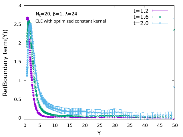
Figure 6: Real part of the boundary term for real-time extents of 1.2, 1.6 and 2.0 from a kernelled CLE simulation with an optimized field-independent kernel.

This behaviour is nicely confirmed on the correlators, shown in Fig. 7. The shortest simulation at $t=1.2$ shows that results agree with the exact results. At $t=1.6$ small deviations from the exact results start to emerge, while at $t=2.0$ we see a clearly non-time translation invariant equal-time two point function and an unequal-time two point function that deviates from the exact one.

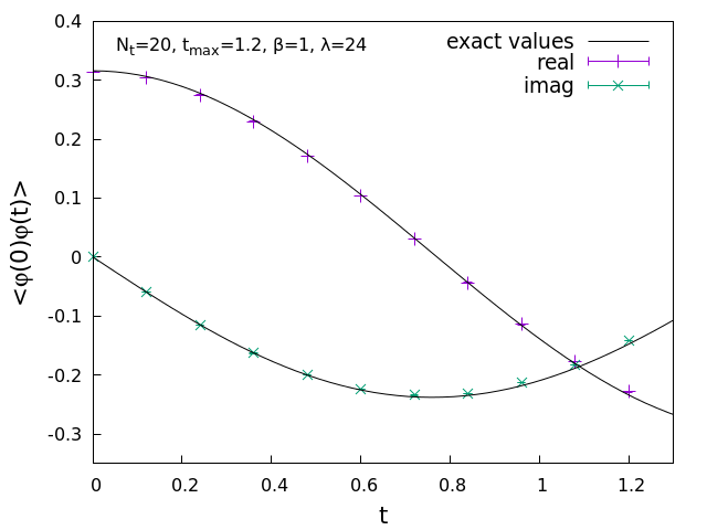
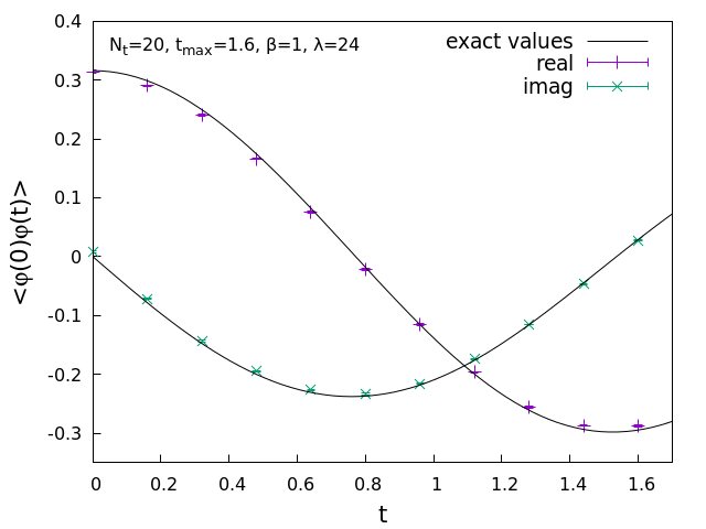
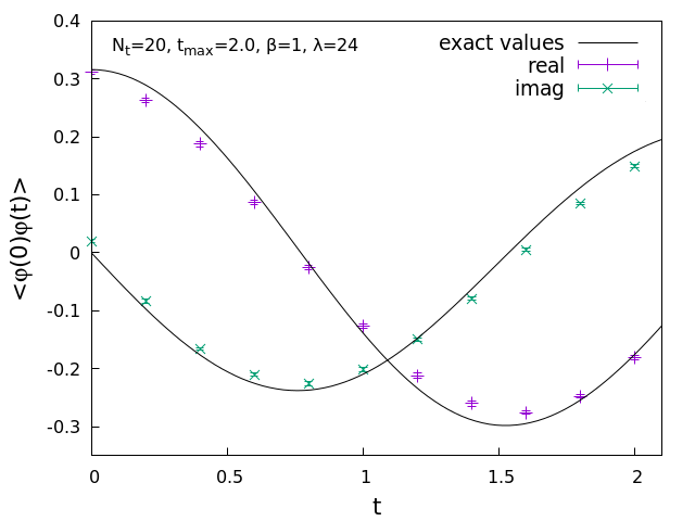
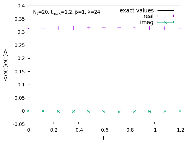
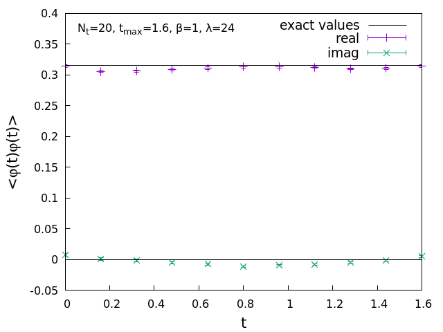
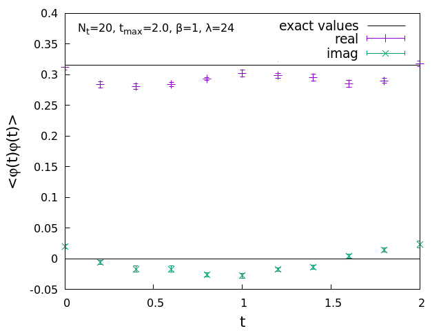
Figure 7: Correlator $\langle\phi(0)\phi(t)\rangle$ (top) and $\langle\phi(t)^{2}\rangle$ (bottom) for optimally kernelled simulations at real time-extents of 1.2, 1.6 and 2.0, respectively. The discretisation used $N_{t}=20$ .

In summary, we have shown in this section that an optimized constant kernel can significantly extend the region of reachable real-time extents for an anharmonic scalar oscillator.

IV Machine Learning for a field dependent kernel

In this section we study field dependent kernels. To keep complications to a minimum, first we study a simple one variable toy model with the action

$$S(x)={1\over 2}\sigma x^{2}+{1\over 4}\lambda x^{4}.$$ (12)

This model was previously investigated in Okano:1991tz . Here we test the model using the parameters $\sigma=-1+4i,\ \lambda=2$, where we have the approximate result $\langle x^{2}\rangle=0.106875-i0.440711$, as calculated by e.g. numerical integration using the trapezoid rule.

To overcome the problem of wrong convergence we introduce a field dependent kernel $K(z)$, such that the CLE is modified to eq. (3). We use various kernels: first, we use the ansatz

$$K(z)=C_{1}e^{-z^{2}/a}e^{-i\Theta_{1}}+C_{2}\left(1-e^{-z^{2}/a}\right)e^{-i\Theta_{2}}$$ (13)

inspired by Okano:1991tz , where parameters $C_{1},\,C_{2},\,\Theta_{1},\,\Theta_{2},\,a$ are to be optimized. (In Okano:1991tz they were chosen explicitly using theoretical considerations.) We use the loss function $N=F_{1}(\textrm{Re}z)^{2}+F_{2}(\textrm{Im}z)^{2}$, and a similar optimization procedure to the one used in section III. In some cases the system achieves a small loss function by simply choosing a small kernel (that is, small $C_{1}$ and $C_{2}$). This is equivalent to using very small Langevin timesteps, which means the field doesn’t have time to grow large and reach larger loss function values. As this is an undesired behavior, we introduced a new term in the loss function which punishes small kernel values. In practice one can use e.g. this expression

$$L_{\textrm{timestep}}={0.01\over\sum_{ij}(\textrm{Re}H_{ij})^{2}+(\textrm{Im}H_{ij})^{2}},$$ (14)

where we used the notation for a general matrix kernel. With this prescription the optimization procedure works well and finds a kernel such that the kernelled CLE delivers results close to the exact results.

Second, we use a neural network to build a $K(z)$ function. The first difficulty that needs to be addressed is the choice of the activation function, as we want to keep a holomorphic kernel. A kernel with some singularities is expected to be acceptable, as long as the process vanishes sufficiently fast near the singularities. A general non-holomorphic kernel, dependent separately on the real and imaginary parts of the field is not expected to work. If one wants to have no singularities on the complex plane (except at infinity), on is basically left with polynomials, exponentials, and combinations (sums or products) thereof. For the purposes of this study, we have chosen the activation function

$$y(z)=e^{-z^{2}/a}.$$ (15)

Note that the universal approximation theorem for complex neural networks does not hold for holomorphic functions voigtlaender2023universal . We also did some experiments with the activation function

$$y(z)={1\over 2}\left(1+\cos(\arg(z))\right)z,$$ (16)

which violates holomorphicity, but the universal approximation theorem is valid voigtlaender2023universal . Similarly to the previous case, we need a term in the loss function which does not allow small kernel values. With an optimization procedure similar to what has been used before, we get results close to the exact ones, however in the case of the non-holomorphic kernel we see significant deviations especially in the imaginary part of the observable $\langle z^{2}\rangle$.

We also investigated field dependent kernels for the real time evolution studied in Section III. The kernels used were of the form $H(\phi)=H_{\textrm{const}}+H_{\textrm{nn}}(\phi)$, where $H_{\textrm{const}}$ is a constant kernel we have first optimized using the procedure in Section III. $H_{nn}(\phi)$ is a field dependent kernel that is given by a neural network. We have chosen again the activation function $\exp(-z^{2})$. The neural network consisted of 4 layers with 32,32,64,and $N_{t}^{2}$ nodes, such that its output can be used as an $N_{t}$ by $N_{t}$ complex matrix. Using this formulation we can efficiently compute the kernel as well as its derivative (which we need for the CLE), with forward and backward propagation on the network. We choose random initial values for the network parameters such that $H_{\textrm{nn}}$ are small.

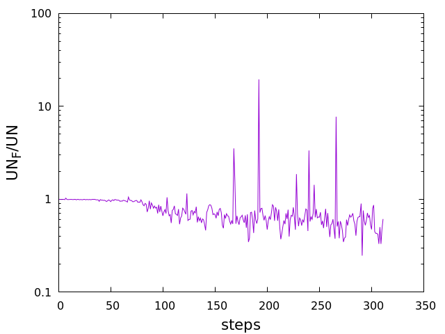
Figure 8: Imaginary norm with a field dependent kernel UN_F divided by the imaginary norm with a field independent kernel UN over optimization steps.

In Fig. 8 we show the behavior of the imaginary norm $N(\phi)=\sum_{x,t}(\textrm{Im}\phi_{t}(x))^{2}$ in ratio to the average imaginary norm with a constant kernel, as the training of the network progresses. One notes that the majority of the values are indeed smaller for the field dependent kernel, however there are huge spikes in the values. This is probably caused by the neural network amplifying the tails of the complexified distributions in the imaginary directions, as $\exp((\textrm{Im}z)^{2})$ is growing rapidly. Unfortunately this also means that expectation values of observables are contaminated by the spikes, and thus are unusable. In summary, field dependent kernels for the real time oscillator are showing promising first results, but more work is definitely needed to solve its problems.

V Conclusions

In this paper we have investigated the application of kernels to solve the problem of the Complex Langevin approach: occasional convergence to incorrect results due to boundary terms or wrong spectral properties of the $L_{c}$ operator Seiler:2023kes .

We studied an anharmonic quantum oscillator in thermal equilibrium on a Schwinger-Keldysh-like complex time-contour. The naive CLE gives correct results at small real-time extents and wrong results at large real-time extents, as confirmed by measurement of the boundary terms, as well as comparison to exact results (calculated by diagonalization of the Hamiltonian). The incorrect results are also signalled by a time dependent equal-time two point function.

Next, we have introduced a constant matrix kernel in the CLE. We have optimized the kernel using stochastic gradient descent by requiring that the distance of the complexified distribution from the real manifold is minimal. This in turn has led to sizeable reduction of the boundary terms. The reachable real-time extent (where the boundary terms are zero within statistical errors) with the optimized kernel is roughly twice as large as with the naive CLE, for the parameters used in this study.

Finally we have explored possibilities of field dependent kernels, for which we use a simple ansatz or we represent them with a neural network. As we want to choose a holomorphic kernel function, this requires a careful choice of the neural network architecture and especially the activation function. We have studied a one variable toy model and we have seen that the optimization procedure used before works also in this case, if the loss function is modified such that low kernel values are avoided (these would correspond to ”slowing” the Langevin dynamics such that field values remain stuck). Promising first results were also gained for the field dependent kernel of the quantum oscillator, however the results we gained tend to have a long tailed distribution, probably caused by large magnitude kernel values, so more work is needed to better understand this behavior, perhaps a different network architecture would be more suitable for the complex kernels. We plan to come back to this issue in a subsequent study.

Note that an independent but similar study has appeared recently Alvestad:2022abf , with similar results and some important differences: The loss function in Alvestad:2022abf used a condition on the drift terms to achieve field-independent kernels such that the drift attracts field values to the origin, and also used boundary terms, symmetries of the system and results from euclidean simulations in the loss function. In contrast, here we use a simpler loss function which just aims at the minimization of the average distance of fields from the real axis (or the origin), and we achieved robust convergence to an optimal kernel. In this study we also report on our first experiments with field dependent kernels.

One of the main advantages of the CLE approach to real-time evolution is the volume scaling of the costs of the simulations, as CLE is expected to scale roughly linearly with the volume, in contrast with the exponential scaling for diagonalization. This makes studying field theories feasible, and an extension of the study of scalar field theory with nonzero spatial extent is already underway arsinprep .

In summary, we have shown that using kernels can decrease boundary terms such that the CLE delivers (within statistical errors) correct results. In particular for the scalar oscillator, an optimized constant kernel allows calculation of the observables on real-time contours that are significantly longer than what the un-kernelled CLE allows. First indications show that field dependent kernels might lead to an even better behavior, however, more work is needed in this line of study.

- (1) A. Rothkopf, Bayesian inference of real-time dynamics from lattice QCD, Front. Phys. 10 (2022) 1028995 [2208.13590].
- (2) C.E. Berger, L. Rammelmüller, A.C. Loheac, F. Ehmann, J. Braun and J.E. Drut, Complex Langevin and other approaches to the sign problem in quantum many-body physics, Phys. Rept. 892 (2021) 1 [1907.10183].
- (3) A. Alexandru, G. Basar, P.F. Bedaque and N.C. Warrington, Complex paths around the sign problem, Rev. Mod. Phys. 94 (2022) 015006 [2007.05436].
- (4) K. Nagata, Finite-density lattice QCD and sign problem: Current status and open problems, Prog. Part. Nucl. Phys. 127 (2022) 103991 [2108.12423].
- (5) J.R. Klauder, STOCHASTIC QUANTIZATION, Acta Phys.Austriaca Suppl. 25 (1983) 251.
- (6) G. Parisi, On complex probabilities, Phys.Lett. B131 (1983) 393.
- (7) F. Attanasio, B. Jäger and F.P.G. Ziegler, Complex Langevin simulations and the QCD phase diagram: Recent developments, Eur. Phys. J. A 56 (2020) 251 [2006.00476].
- (8) H. Huffel and H. Rumpf, Stochastic Quantization in Minkowski Space, Phys. Lett. B 148 (1984) 104.
- (9) D.J.E. Callaway, F. Cooper, J.R. Klauder and H. Rose, Langevin Simulations in Minkowski Space, Nucl. Phys. B 262 (1985) 19.
- (10) H. Nakazato and Y. Yamanaka, MINKOWSKI STOCHASTIC QUANTIZATION, Phys. Rev. D 34 (1986) 492.
- (11) J. Berges and I.-O. Stamatescu, Simulating nonequilibrium quantum fields with stochastic quantization techniques, Phys. Rev. Lett. 95 (2005) 202003.
- (12) J. Berges, S. Borsanyi, D. Sexty and I.O. Stamatescu, Lattice simulations of real-time quantum fields, Phys. Rev. D 75 (2007) 045007 [hep-lat/0609058].
- (13) J. Berges and D. Sexty, Real-time gauge theory simulations from stochastic quantization with optimized updating, Nucl. Phys. B799 (2008) 306 [0708.0779].
- (14) A. Alexandru, G. Basar, P.F. Bedaque, S. Vartak and N.C. Warrington, Monte Carlo Study of Real Time Dynamics on the Lattice, Phys. Rev. Lett. 117 (2016) 081602 [1605.08040].
- (15) AuroraScience collaboration, New approach to the sign problem in quantum field theories: High density QCD on a Lefschetz thimble, Phys.Rev. D86 (2012) 074506 [1205.3996].
- (16) B. Soderberg, On the Complex Langevin Equation, Nucl. Phys. B295 (1988) 396.
- (17) H. Okamoto, K. Okano, L. Schulke and S. Tanaka, The Role of a Kernel in Complex Langevin Systems, Nucl. Phys. B324 (1989) 684.
- (18) K. Okano, L. Schulke and B. Zheng, Kernel controlled complex Langevin simulation: Field dependent kernel, Phys. Lett. B258 (1991) 421.
- (19) D. Alvestad, R. Larsen and A. Rothkopf, Towards learning optimized kernels for complex Langevin, JHEP 04 (2023) 057 [2211.15625].
- (20) K. Boguslavski, P. Hotzy and D.I. Müller, Stabilizing complex Langevin for real-time gauge theories with an anisotropic kernel, JHEP 06 (2023) 011 [2212.08602].
- (21) G. Aarts, E. Seiler and I.-O. Stamatescu, The Complex Langevin method: When can it be trusted?, Phys.Rev. D81 (2010) 054508 [0912.3360].
- (22) G. Aarts, F.A. James, E. Seiler and I.-O. Stamatescu, Complex Langevin: Etiology and Diagnostics of its Main Problem, Eur.Phys.J. C71 (2011) 1756 [1101.3270].
- (23) G. Aarts, E. Seiler, D. Sexty and I.-O. Stamatescu, Complex Langevin dynamics and zeroes of the fermion determinant, JHEP 05 (2017) 044 [1701.02322].
- (24) E. Seiler, D. Sexty and I.-O. Stamatescu, Complex Langevin: Correctness criteria, boundary terms and spectrum, 2304.00563.
- (25) M. Scherzer, E. Seiler, D. Sexty and I.-O. Stamatescu, Complex Langevin and boundary terms, Phys. Rev. D99 (2019) 014512 [1808.05187].
- (26) M. Scherzer, E. Seiler, D. Sexty and I.O. Stamatescu, Controlling Complex Langevin simulations of lattice models by boundary term analysis, Phys. Rev. D 101 (2020) 014501 [1910.09427].
- (27) G.G. Batrouni, G.R. Katz, A.S. Kronfeld, G.P. Lepage, B. Svetitsky and K.G. Wilson, Langevin Simulations of Lattice Field Theories, Phys. Rev. D 32 (1985) 2736.
- (28) G. Aarts, F.A. James, J.M. Pawlowski, E. Seiler, D. Sexty and I.-O. Stamatescu, Stability of complex Langevin dynamics in effective models, JHEP 03 (2013) 073 [1212.5231].
- (29) F. Voigtlaender, The universal approximation theorem for complex-valued neural networks, Applied and Computational Harmonic Analysis 64 (2023) 33.
- (30) D. Alvestad, A. Rothkopf and D. Sexty, Lattice real-time simulations with learned optimal kernels, in preparation (2023) .