$L^{q}$-spectra of box-like graph-directed self-affine measures: closed forms, with rotation

Abstract.

We consider $L^{q}$-spectra of planar graph-directed self-affine measures generated by diagonal or anti-diagonal matrices. Assuming the directed graph is strongly connected and the system satisfies the rectangular open set condition, we obtain a general closed form expression for the $L^{q}$-spectra. Consequently, we obtain a closed form expression for box dimensions of associated planar graph-directed box-like self-affine sets. We also provide a precise answer to a question of Fraser in 2016 concerning the $L^{q}$-spectra of planar self-affine measures generated by diagonal matrices.

1. Introduction

Let $\{T_{1},\cdots,T_{N}\}$ be a finite collection of affine contracting non-singular matrices, and let $\Psi=\{\psi_{i}(\cdot)=T_{i}(\cdot)+t_{i}\}_{i=1}^{N}$ be an iterated function system (IFS) with $t_{i}\in\mathbb{R}^{n}$ for all $i\in\{1,\cdots,N\}$. It is well known that there exists a unique non-empty compact set $X$ such that

$$X=\bigcup_{i=1}^{N}\psi_{i}(X).$$

We call $\Psi$ a self-affine IFS and $X$ a self-affine set. In the special case when $T_{i}$’s are all similarities, call $\Psi$ a self-similar IFS and $X$ a self-similar set.

For a positive probability vector $\mathcal{P}=(p_{i})_{i=1}^{N}$, there exists a probability measure $\mu$ satisfying

$$\mu=\sum_{i=1}^{N}p_{i}\cdot\mu\circ\psi_{i}^{-1}.$$

Call $\mu$ a self-affine measure (resp. self-similar measure) when $\Psi$ is a self-affine IFS (resp. self-similar IFS).

The dimension theory of self-affine sets or measures is one of central problems in fractal geometry. Historically, there are two basic strands to determine the Hausdorff and box dimensions of self-affine sets, one of which is to study generic self-affine sets basing on the singular value functions, and to make almost sure statements

$$\dim_{H}X=\dim_{B}X=d(T_{1},\cdots,T_{N})\text{ for Lebesgue-almost sure }\textbf{t}=(t_{1},\cdots,t_{N})\in\mathbb{R}^{nN},$$

pioneered by Falconer [9]. The critical number $d(T_{1},\cdots,T_{N})$, called affinity dimension, is determined in terms of singular values of $\{T_{1},\cdots,T_{N}\}$. The original consideration of Falconer requires that all norms of $T_{i}$’s are less than $1/3$, which was later improved by Solomyak [46] to $1/2$ and the constant $1/2$ is proved to be sharp in [7, 46]. Along this direction, the study is thriving, see [24, 2, 12, 39, 37, 4, 19] and the references therein.

The other strands of study is to focus on special classes of self-affine sets, and to determine sure statements for the dimensions of attractors, which was pioneered by McMullen [35] and Bedford [3], considering planar box-like self-affine sets with homogeneous grid structure. Their approaches were further developed by Lalley and Gatzouras [30] and Barański [1] to box-like sets with certain geometric arrangement or general grid structure. See [27, 8, 29, 23] for extensions to high dimensions.

The planar box-like self-affine sets without grid structure were firstly considered by Feng and Wang [16], and later extended by Fraser [20, 21] allowing the IFS’s have non-trivial rotations and reflections (later called self-affine carpets), i.e. linear parts of maps were allowed to be diagonal or anti-diagonal. All these works [16, 20, 21] on self-affine carpets focus on computing the $L^{q}$-spectra of their associated self-affine measures. See also [11] for an extension to non-conformal measures.

In this paper, we continue to study the $L^{q}$-spectra of self-affine measures. Let $\nu$ be a compactly supported Borel probability measure on $\mathbb{R}^{n}$ with $n\geq 1$. For $\delta>0$, let $\mathcal{M}_{\delta}$ be the collection of closed cubes in the $\delta$-mesh of $\mathbb{R}^{n}$. For $q\geq 0$, write

$$\mathcal{D}_{\delta}^{q}(\nu)=\sum_{Q\in\mathcal{M}_{\delta}}\nu(Q)^{q}.$$

Definition 1.1.

For $q\geq 0$, the upper and lower $L^{q}$-spectra of $\nu$ are defined to be

$$\overline{\tau}_{\nu}(q)=\limsup_{\delta\to 0+}\frac{\log\mathcal{D}_{\delta}^{q}(\nu)}{-\log\delta}$$

and

$$\underline{\tau}_{\nu}(q)=\liminf_{\delta\to 0+}\frac{\log\mathcal{D}_{\delta}^{q}(\nu)}{-\log\delta},$$

respectively. If these two values coincide, we define the $L^{q}$-spectra of $\nu$ to be their common value, and denote it as $\tau_{\nu}(q)$.

It is known that as functions of $q$, both $\underline{\tau}_{\nu}(q),\overline{\tau}_{\nu}(q)$ are decreasing, and equal to zero at $q=1$. Also, they are convex, continuous on $(0,\infty)$, and Lipschitz on $[\lambda,\infty)$ for any $\lambda>0$. Note that when $q=0$, the upper and lower $L^{q}$-spectra are equal to the upper and lower box dimensions of $supp\nu$, respectively. Another important property of $L^{q}$-spectra is that if it is differential at $q=1$, then the measure $\nu$ is exactly dimensional, and the Hausdorff dimension of $\nu$ equals to $-\tau^{\prime}(1)$. The concept of $L^{q}$-spectra is an important fundamental ingredient in the study of fractal geometry, particularly in multifractal analysis. See [31, 13, 15, 33, 14, 28, 43, 10] and references therein for more details.

For a self-similar measure $\mu$ with probability vector $\mathcal{P}=(p_{i})_{i=1}^{N}$, for $q\in\mathbb{R}$, the $L^{q}$-spectrum of $\mu$ is given by a closed form expression that

$$\sum_{i=1}^{N}p_{i}^{q}r_{i}^{\tau_{\mu}(q)}=1,$$ (1.1)

where $r_{i}$ is the contraction ratio of $\psi_{i}$. See Cawley and Mauldin [5] and Olsen [42].

For self-affine measures, Feng and Wang [16, Theorem 2] obtained the analogous closed form expression for diagonal self-affine carpets in terms of the $L^{q}$-spectra of the projections of measures onto $y$-axis providing that the contraction ratios on $x$-axis are less than on $y$-axis for all elements in the IFS’s. In a different way, Fraser [21] introduced the concept of modified singular value functions (modified from Falconer’s original definition [9]), and used which to compute the closed form expression for $L^{q}$-spectra of self-affine measures on self-affine carpets without limitation of relative sizes of contraction ratios on $x$-axis or $y$-axis, but still requiring that all $T_{i}$’s are diagonal.

In their setting, all $T_{i}$’s are of the form $T_{i}=diag\{\pm a_{i},\pm b_{i}\}$ with $0<a_{i},b_{i}<1$. Let $\gamma_{A}(q),\gamma_{B}(q)$ be the unique solutions of

$$\sum_{i=1}^{N}p_{i}^{q}a_{i}^{\tau_{\mu^{x}}(q)}b_{i}^{\gamma_{A}(q)-\tau_{\mu^{x}}(q)}=1$$

and

$$\sum_{i=1}^{N}p_{i}^{q}a_{i}^{\gamma_{B}(q)-\tau_{\mu^{y}}(q)}b_{i}^{\tau_{\mu^{y}}(q)}=1,$$

where $\mu^{x}$(resp. $\mu^{y}$) is the projection of $\mu$ onto $x$-axis (resp. $y$-axis). The result in [21] states that $\tau_{\mu}(q)=\max\{\gamma_{A}(q),\gamma_{B}(q)\}$ if $\max\{\gamma_{A}(q),\gamma_{B}(q)\}\leq\tau_{\mu^{x}}(q)+\tau_{\mu^{y}}(q)$, and

$$\tau_{\mu}(q)\leq\min\{\gamma_{A}(q),\gamma_{B}(q)\}$$

if $\min\{\gamma_{A}(q),\gamma_{B}(q)\}\geq\tau_{\mu^{x}}(q)+\tau_{\mu^{y}}(q)$ and equality occurs if

$$\textit{ either }\sum_{i=1}^{N}p_{i}^{q}a_{i}^{\tau_{\mu^{x}}(q)}b_{i}^{\gamma_{A}(q)-\tau_{A}(q)}\log a_{i}/b_{i}\geq 0,$$ (1.2a)

$$\textit{ or }\sum_{i=1}^{N}p_{i}^{q}b_{i}^{\tau_{\mu^{y}}(q)}a_{i}^{\gamma_{B}(q)-\tau_{\mu^{y}}(q)}\log a_{i}/b_{i}\leq 0.$$ (1.2b)

Naturally it remains a question [21, Question 2.14] raised by Fraser that whether the additional condition (1.2) can be removed, i.e.

Question 1.2 ([21, Question 2.14]).

When $\min\{\gamma_{A}(q),\gamma_{B}(q)\}\geq\tau_{\mu^{x}}(q)+\tau_{\mu^{y}}(q)$, is

$$\tau_{\mu}(q)=\min\{\gamma_{A}(q),\gamma_{B}(q)\}$$

still true if (1.2) dose not hold?

This question was answered by Fraser, Lee, Morris and Yu [22] in the negative by a special family of counterexamples. In particular, they consider a family of diagonal systems consisting of two maps equipped with a Bernoulli-$(1/2,1/2)$ measure. For this family, it may really happen that

$$\tau_{\mu}(q)<\min\{\gamma_{A}(q),\gamma_{B}(q)\}$$ (1.3)

for all $q>1$, and the exact expression of $\tau_{\mu}(q)$ was obtained recently by Kolossváry [29, Proposition 4.4] in the setting that grid structure of carpets (could be in high dimensional) are required.

Nevertheless, it remains unclear that:

$\bullet$ What is the general exact expression of $\tau_{\mu}(q)$ when $\min\{\gamma_{A}(q),\gamma_{B}(q)\}\geq\tau_{\mu^{x}}(q)+\tau_{\mu^{y}}(q)$?

$\bullet$ What is the general comparison between the values of $\tau_{\mu}(q)$ and $\min\{\gamma_{A}(q),\gamma_{B}(q)\}$?

All the above considerations require that maps in IFS’s are diagonal.

$\bullet$ What would it be when allowing maps in IFS’s to be anti-diagonal?

Along this direction, Morris [38, Proposition 5] derived a closed form expression for box dimensions (taking $q=0$ in $\tau_{\mu}(q)$) for self-affine carpets, requiring that at least one of $T_{i}$’s in IFS’s is anti-diagonal.

Figure 1. An example of graph-directed self-affine carpet families.

Our main aim in this paper is to answer the above questions. We will extend the consideration from the IFS setting to the more general graph-directed IFS (GIFS) setting, allowing contracting maps to be either diagonal or anti-diagonal, i.e. each associated matrix $T_{i}$ is of the form

$$T_{i}=\left(\begin{array}[]{cc}\pm a_{i}&0\\ 0&\pm b_{i}\\ \end{array}\right)\text{ or }\left(\begin{array}[]{cc}0&\pm a_{i}\\ \pm b_{i}&0\\ \end{array}\right).$$

See Figure 1 for an example of associated graph-directed self-affine carpet families. We will obtain a general exact closed form expression for $L^{q}$-spectra of graph-directed self-affine measures, for general $q\geq 0$. Specifically, returning to the diagonal IFS setting concerned by Question 1.2, our result will state that the strict inequality (1.3) generally holds when (1.2) does not hold. Indeed, we will prove when $\min\{\gamma_{A}(q),\gamma_{B}(q)\}\geq\tau_{\mu^{x}}(q)+\tau_{\mu^{y}}(q)$,

$$\tau_{\mu}(q) =\min\{x+y:\sum_{i=1}^{N}p_{i}^{q}a_{i}^{x}b_{i}^{y}=1,\tau_{A}(q)\leq x\leq\gamma_{B}(q)-\tau_{B}(q)\}$$ (1.4)

$$=\left\{\begin{aligned} &\gamma_{A}(q)&\quad&\text{ if \eqref{e90a} holds},\\ &\gamma_{B}(q)&\quad&\text{ if \eqref{e90b} holds},\\ &<\min\{\gamma_{A}(q),\gamma_{B}(q)\}&\quad&\textit{otherwise. }\end{aligned}\right.$$

Not only that, we will illustrate that the above expression can alternatively be directly derived from Feng and Wang’s original result [16, Theorem 1] by using a careful Lagrange multipliers method. Another improvement of (1.4) is that it specifies the necessary and sufficient condition that $\tau_{\mu}(q)$ equals to $\gamma_{A}(q)$ (resp. $\gamma_{B}(q)$), compared with that in [21].

When allowing some maps to be anti-diagonal, our result is also a non-trivial extension of that of Morris’s [38] for box dimension (the $q=0$ case) to all $q\geq 0$ and to the GIFS setting. In his IFS setting, the graph-directed self-affine measure family degenerates to a single measure $\mu$. The requirement that at least one of $T_{i}$’s in the IFS is anti-diagonal ensures that $\tau_{\mu^{x}}(0)=\tau_{\mu^{y}}(0)$ (taking $q=0$) since $\{\mu^{x},\mu^{y}\}$ becomes a strongly connected graph-directed self-similar measure family. However, in the GIFS setting, the graph-directed self-affine measure family $\{\mu_{v}\}_{v}$ will generate a collection of projection measures $\{\mu_{v}^{x},\mu_{v}^{y}\}_{v}$, which will be proved to be a disjoint union of one or two strongly connected self-similar measure families, and consequently it may happen that $\tau_{\mu_{v}^{x}}(0)\neq\tau_{\mu_{v}^{y}}(0)$. This will cause the main difficulty in GIFS setting. Another main difficulty is to properly divide the consideration into distinct cases for distinct $q\geq 0$.

The motivation that we extend the consideration to the GIFS setting is the potential application that we can use which to consider box-like self-affine IFS’s of finite overlapping types, analogous to that of Ngai and Wang [40] and the extension [32] for self-similar IFS’s. We illustrate this in a recent paper [44] concerning the $L^{q}$-spectra for lower triangular planar non-conformal measures. We mention that there are also some previous works in box-like self-affine GIFS setting. In [26], Kenyon and Peres extended the results of Bedford [3] and McMullen [35] computing the Hausdorff and box dimensions of graph-directed self-affine carpets with homogeneous grid structure. In [41], Ni and Wen considered the $L^{q}$-spectra for graph-directed self-affine measures on Feng and Wang’s sets [16], in the setting that contraction ratios on $x$-axis are always less than that on $y$-axis for all maps in the GIFS’s, but additionally requiring contraction ratios on $x$-axis to be arithmetic.

Basic setting and notations.

The concept of graph-directed iterated function system (GIFS) was firstly introduced by Mauldin and Williams [34].

Let $(V,E)$ be a finite directed graph with $V$ being the vertex set and $E$ being the directed edge set, allowing loops and multiple edges. For $e\in E$, denote by $i(e)$ the initial vertex, $t(e)$ the terminal vertex of $e$, and sometimes write this as $i(e)\stackrel{{\scriptstyle e}}{{\rightarrow}}t(e)$. We always assume that for each $v\in V$, there exists at least one edge $e\in E$ satisfying $i(e)=v$.

Denote the collection of all finite admissible words by

$$E^{*}=\{w=w_{1}\cdots w_{k}:t(w_{i-1})=i(w_{i}),\forall 1<i\leq k,k\in\mathbb{N}\}.$$

For $w=w_{1}\cdots w_{k}\in E^{*}$, denote $|w|=k$ the length of $w$, $i(w)=i(w_{1})$, $t(w)=t(w_{k})$ the initial and terminal vertices of $w$, and also write $i(w)\stackrel{{\scriptstyle w}}{{\rightarrow}}t(w)$. For $w,w^{\prime}\in E^{*}$ with $t(w)=i(w^{\prime})$, write $ww^{\prime}$ the concatenation of $w$ and $w^{\prime}$, and call $w$ a prefix of $ww^{\prime}$. Denote $E^{k}$ the collection of all admissible words of length $k\geq 1$.

For $v,v^{\prime}\in V$, we say that there exists a directed path from $v$ to $v^{\prime}$ if there exists $w\in E^{*}$ satisfying $v\stackrel{{\scriptstyle w}}{{\rightarrow}}v^{\prime}$ (write simply $v\to v^{\prime}$ when we do not emphasize $w$). Write $v\nrightarrow v^{\prime}$ if there is not a directed path form $v$ to $v^{\prime}$. We say $(V,E)$ is strongly connected (or irreducible), if $v\to v^{\prime}$ for all pairs $v,v^{\prime}\in V$.

For each $e\in E$, we assume that there exists a contraction $\psi_{e}$ in the form of $\psi_{e}(\cdot)=T_{e}(\cdot)+t_{e}$, where $T_{e}$ is an $n\times n$ affine contracting matrix and $t_{e}\in\mathbb{R}^{n}$. We write $\Psi=\{\psi_{e}\}_{e\in E}$ the collection of all contractions $\psi_{e}$’s. Call the triple $(V,E,\Psi)$ a self-affine GIFS. It is well known that there exists a unique family of compact sets $\{X_{v}\}_{v\in V}$ satisfying

$$X_{v}=\bigcup_{e\in E:i(e)=v}\psi_{e}(X_{t(e)}),\quad\text{for all }v\in V.$$

We call $\{X_{v}\}_{v\in V}$ a graph-directed self-affine set family associated with $(V,E,\Psi)$. Note that if $V$ is a singleton, $(V,E,\Psi)$ degenerates to a self-affine IFS and $\{X_{v}\}_{v\in V}$ degenerates to a self-affine set $X$.

Let $\mathcal{P}=(p_{e})_{e\in E}$ be a positive vector satisfying

$$\sum_{e\in E:i(e)=v}p_{e}=1,\quad\text{for all }v\in V.$$ (1.5)

It is known that there exists a unique finite family of probability measures $\{\mu_{v}\}_{v\in V}:=\{\mu_{\mathcal{P},v}\}_{v\in V}$ supported on $\{X_{v}\}_{v\in V}$ such that

$$\mu_{v}=\sum_{e\in E:i(e)=v}p_{e}\cdot\mu_{t(e)}\circ\psi_{e}^{-1},\quad\text{for all }v\in V.$$

We call $\{\mu_{v}\}_{v\in V}$ a graph-directed self-affine measure family associated with $\mathcal{P}$.

Throughout the paper, we assume that for each $e\in E$, $T_{e}$ is a $2\times 2$ diagonal or anti-diagonal matrix of the form

$$T_{e}=\left(\begin{array}[]{cc}\pm a_{e}&0\\ 0&\pm b_{e}\\ \end{array}\right)\text{ or }\left(\begin{array}[]{cc}0&\pm a_{e}\\ \pm b_{e}&0\\ \end{array}\right)$$ (1.6)

where $0<a_{e},b_{e}<1$. We call $(V,E,\Psi)$ a planar box-like self-affine GIFS, $\{X_{v}\}_{v\in V}$ a graph-directed self-affine carpet family associated with $(V,E,\Psi)$ and $\{\mu_{v}\}_{v\in V}$ a graph-directed box-like self-affine measure family. See Figures 2-3 for an example.

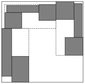
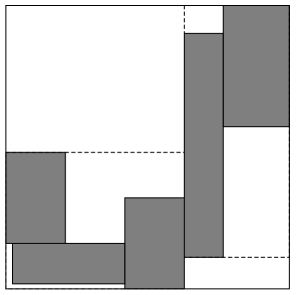
Figure 2. A planar box-like self-affine GIFS with $\#V=2,\#E=5$. Images of $[0,1]^{2}$ under the first and second level iterations of maps in the GIFS.

Figure 3. The graph-directed self-affine carpet family generated by the GIFS in Figure 2.

In this paper, we care about the $L^{q}$-spectra of strongly connected planar graph-directed box-like self-affine measures $\{\mu_{v}\}_{v\in V}$. For calculating the $L^{q}$-spectra, we need the following separating condition for the planar box-like self-affine GIFS’s, which was firstly proposed by Feng and Wang [16] and plays crucial roles in subsequent works [20, 21, 22, 11].

Definition 1.3 (Rectangular open set condition).

We say a planar box-like self-affine GIFS $(V,E,\Psi)$ satisfies the rectangular open set condition (ROSC) if for all $v$ in $V$,

$$\bigcup_{e\in E:i(e)=v}\psi_{e}((0,1)^{2})\subseteq(0,1)^{2}$$

and the union is disjoint.

Our results rely on the $L^{q}$-spectra of the projections of measures onto $x$-axis or $y$-axis. Let $\pi_{x}$, $\pi_{y}:\mathbb{R}^{2}\to\mathbb{R}$ be defined by $\pi_{x}(\xi_{1},\xi_{2})=\xi_{1}$ and $\pi_{y}(\xi_{1},\xi_{2})=\xi_{2}$ for $(\xi_{1},\xi_{2})\in\mathbb{R}^{2}$, respectively. For each $v$ in $V$, define

$$\mu_{v}^{x}=\mu_{v}\circ\pi_{x}^{-1},\quad\mu_{v}^{y}=\mu_{v}\circ\pi_{y}^{-1}$$

the projection measures of $\mu_{v}$ onto $x$-axis and $y$-axis. Note that $\{\mu_{v}^{x},\mu_{v}^{y}\}_{v\in V}$ is a family of graph-directed self-similar measures.

Proposition 1.4 ([21, Theorem 2.1]).

For a strongly connected graph-directed self-similar measure family $\{\nu_{v}\}_{v\in V}$, for all $q\geq 0$ and $v,v^{\prime}\in V$, we have

$$\underline{\tau}_{\nu_{v}}(q)=\overline{\tau}_{\nu_{v}}(q)=\underline{\tau}_{\nu_{v^{\prime}}}(q)=\overline{\tau}_{\nu_{v^{\prime}}}(q),$$

i.e. the $L^{q}$-spectra exist and are the same for all $\nu_{v}$’s.

When $(V,E)$ is strongly connected and all $T_{e}$’s are diagonal, both $\{\mu_{v}^{x}\}_{v\in V}$ and $\{\mu_{v}^{y}\}_{v\in V}$ are two strongly connected graph-directed self-similar measure families; when $V$ is a singleton and $T_{e}$ is anti-diagonal for some $e\in E$, $\{\mu_{v}^{x},\mu_{v}^{y}\}_{v\in V}$ is a strongly connected graph-directed self-similar measure family; for general strongly connected case, $\{\mu_{v}^{x},\mu_{v}^{y}\}_{v\in V}$ can be divided into one or two families of strongly connected graph-directed self-similar measures (see Proposition 2.1). By Proposition 1.4, we always have the $L^{q}$-spectra exist for all $\mu_{v}^{x}$’s, $\mu_{v}^{y}$’s.

Throughout the paper, we will write $a\lesssim b$ for two variables (functions) if there is a constant $C>0$ such that $a\leq C\cdot b$, and write $a\asymp b$ if both $a\lesssim b$ and $b\lesssim a$ hold. We write $a\lesssim_{\theta}b$ to mean that the constant depends on some parameter $\theta$. Similarly, write $a\asymp_{\theta}b$ if both $a\lesssim_{\theta}b$ and $b\lesssim_{\theta}a$ hold. For two vectors $u=(u_{i})$ and $v=(v_{i})$, we write $u\geq v$ if all $u_{i}\geq v_{i}$. Also for two matrices $A=(a_{ij})$ and $B=(b_{ij})$, we write $A\geq B$ if all $a_{ij}\geq b_{ij}$. For a $N\times N$ matrix $A$, for indices $\{i_{1},\cdots,i_{k}\},\{j_{1},\cdots,j_{l}\}$ with $k,l\leq N$, we write $A[\{i_{1},\cdots,i_{k}\},\{j_{1},\cdots,j_{l}\}]$ for a submatrix of $A$ (lying in rows $\{i_{1},\cdots,i_{k}\}$ and columns $\{j_{1},\cdots,j_{l}\}$). We always denote $\|\cdot\|$ the $1$-norm of a matrix, i.e. $\|A\|=\sum_{i,j}|a_{ij}|$.

2. Results

In this section, we list the results in the paper but postpone their proofs to later sections. Our main aim is to obtain the closed form expression for the $L^{q}$-spectra of planar graph-directed box-like self-affine measures.

Throughout the following, we always let $(V,E,\Psi)$ be a strongly connected planar box-like self-affine GIFS, $\mathcal{P}$ be a positive vector satisfying (1.5), and $\{\mu_{v}\}_{v\in V}$ be a graph-directed box-like self-affine measure family associated with $(V,E,\Psi)$ and $\mathcal{P}$. Note that for each $e\in E$, there exists a contraction $\psi_{e}$ in the form of $\psi_{e}(\cdot)=T_{e}(\cdot)+t_{e}$ for some $2\times 2$ diagonal or anti-diagonal contracting matrix $T_{e}$ and $t_{e}\in\mathbb{R}^{2}$. For $v\in V$, we use $\mu_{v}^{x}$ (resp. $\mu_{v}^{y}$) to denote the projection of $\mu_{v}$ onto $x$-axis (resp. $y$-axis).

We will separate our consideration basing on two basic settings:

first, assume all $T_{e}$’s are diagonal;

then, extend the consideration to general case, i.e. allowing some $T_{e}$’s to be anti-diagonal.

Before proceeding, we will prove in general that the $L^{q}$-spectra of measures $\tau_{\mu_{v}^{x}}(q)$, $\tau_{\mu_{v}^{y}}(q)$ and $\tau_{\mu_{v}}(q)$ exist for all $q\geq 0$ and $v\in V$, which will play fundamental roles in our later consideration. We will achieve this through the following Proposition 2.1 and Theorem 2.2 dealing with projection measures and original measures separately.

Proposition 2.1.

Let $(V,E,\Psi)$ be a strongly connected planar box-like self-affine GIFS, $\mathcal{P}$ be an associated positive vector, and $\{\mu_{v}\}_{v\in V}$ be an associated graph-directed box-like self-affine measure family. Then

$$\tau_{\mu_{v}^{x}}(q)\text{ and }\tau_{\mu_{v}^{y}}(q)\text{ exist }\quad\text{ for all }q\geq 0,v\in V.$$ (2.1)

Moreover, $\{\mu_{v}^{x},\mu_{v}^{y}\}_{v\in V}$ can be divided into two disjoint families $A$ and $B$ so that

$$\#A=\#B=\#V,$$

for all $q\geq 0$ there exist $\tau_{A}(q),\tau_{B}(q)$ satisfying

$$\tau_{\nu}(q)=\tau_{A}(q)\quad\text{ for all }\nu\in A,$$ (2.2)

$$\tau_{\nu}(q)=\tau_{B}(q)\quad\text{ for all }\nu\in B,$$

and for all $v\in V$,

$$\text{ either }\quad\mu_{v}^{x}\in A,\mu_{v}^{y}\in B\quad\text{ or }\quad\mu_{v}^{x}\in B,\mu_{v}^{y}\in A.$$ (2.3)

In particular, when all $T_{e}$’s are diagonal, we could take

$$A=\{\mu_{v}^{x}\}_{v\in V}\text{ and }B=\{\mu_{v}^{y}\}_{v\in V}.$$

Due to Proposition 2.1, for $q\geq 0$, $v\in V$, $e\in E$, throughout the paper, we will write

$$\tau_{x,v}(q) :=\tau_{\mu_{v}^{x}}(q)\quad \tau_{y,v}(q):=\tau_{\mu_{v}^{y}}(q),$$ and

$$\tau_{x,e}(q) :=\tau_{x,t(e)}(q) \tau_{y,e}(q):=\tau_{y,t(e)}(q).$$ and

for short. Also, write

$$t(q):=\tau_{A}(q)+\tau_{B}(q)$$

for later use. Clearly, for all $v\in V$, $\tau_{x,v}(q)+\tau_{y,v}(q)=t(q)$.

Next, with Proposition 2.1 in hand, inspired by Fraser’s works [21, 20] dealing with the self-affine carpets, i.e. the case that $(V,E)$ degenerates to a singleton, we will introduce (in Section 3) a pressure function in graph-directed setting,

$$P:\mathbb{R}\times[0,\infty)\to\mathbb{R},$$

basing on certain modified singular value function matrices. For each $q\geq 0$, as a function of $s$, $P(s,q)$ will be strictly decreasing and continuous, tending to $0$ as $s\to+\infty$ and to $+\infty$ as $s\to-\infty$. Using this we will define a function $\gamma:[0,\infty)\to\mathbb{R}$ by setting

$$P(\gamma(q),q)=1.$$

Theorem 2.2.

Let $(V,E,\Psi)$ be a strongly connected planar box-like self-affine GIFS satisfying ROSC, $\mathcal{P}$ be an associated positive vector, and $\{\mu_{v}\}_{v\in V}$ be an associated graph-directed box-like self-affine measure family. Then for all $q\geq 0$ and $v\in V$, $\tau_{\mu_{v}}(q)$ exist and equal to $\gamma(q)$.

Proposition 2.1 will be proved in Section 3. The details for pressure function $P$ will be presented also in Section 3. The proof of Theorem 2.2 will be postponed to Section 6.

From definition, for $q\geq 0$, $\gamma(q)$ does not seem to be able to be explicitly computed through a finite amount of steps. So our next aim attributes to find a closed form expression for $\gamma(q)$, we will separate our consideration into two parts.

Non-rotational setting.

First we will assume that all $T_{e}$’s are diagonal matrices, i.e. each $T_{e}$ is of the form

$$T_{e}=\left(\begin{array}[]{cc}\pm a_{e}&0\\ 0&\pm b_{e}\\ \end{array}\right).$$

In this setting, by Proposition 2.1, $A=\{\mu_{v}^{x}\}_{x\in V}$, $B=\{\mu_{v}^{y}\}_{v\in V},$ and for all $v\in V$, $\tau_{x,v}(q)=\tau_{A}(q)$, $\tau_{y,v}(q)=\tau_{B}(q)$ and $\tau_{x,v}(q)+\tau_{y,v}(q)=t(q).$ For $q\geq 0$, $x,y\in\mathbb{R}$, we will introduce (in Section 4) a $\#E\times\#E$ function matrix $F^{(q)}_{x,y}$ with entries defined by

$$F^{(q)}_{x,y}(e,e^{\prime})=\left\{\begin{aligned} &p_{e^{\prime}}^{q}a_{e^{\prime}}^{x}b_{e^{\prime}}^{y}&\quad&\text{ if }t(e)=i(e^{\prime}),\\ &0&\quad&\text{ otherwise}.\end{aligned}\right.$$ (2.4)

Then define two functions $\gamma_{A},\gamma_{B}:[0,\infty]\to\mathbb{R}$ such that for $q\geq 0$, $\gamma_{A}(q)$ and $\gamma_{B}(q)$ are the unique solutions of

$$\rho(F^{(q)}_{\tau_{A}(q),\gamma_{A}(q)-\tau_{A}(q)})=1$$ (2.5)

and

$$\rho(F^{(q)}_{\gamma_{B}(q)-\tau_{B}(q),\tau_{B}(q)})=1,$$ (2.6)

respectively (to be well-defined in Section 4), where $\rho(\cdot)$ is the spectral radius of a matrix. For fixed $q\geq 0$, for $x\in\mathbb{R}$, we will prove that there exists a unique $y(x)\in\mathbb{R}$ satisfying $\rho(F^{(q)}_{x,y(x)})=1$ and introduce a positive unit row vector $f^{(q)}(x)=(f^{(q)}_{e}(x))_{e\in E}$ (in Section 4).

Theorem 2.3.

Let $(V,E,\Psi)$, $\mathcal{P}$, $\{\mu_{v}\}_{v\in V}$ and $\gamma$ be same as in Theorem 2.2. Assume that all $T_{e}$’s are diagonal. Then for $q\geq 0$,

$$\text{ either }\max\{\gamma_{A}(q),\gamma_{B}(q)\}\leq t(q)$$ (2.7a)

$$\text{ \hskip 5.69046pt or \hskip 11.38092pt}\min\{\gamma_{A}(q),\gamma_{B}(q)\}\geq t(q).$$ (2.7b)

• If (2.7a) holds,

  $$\gamma(q) =\max\{\gamma_{A}(q),\gamma_{B}(q)\}$$ (2.8)

  $$=\max\{x+y:\rho(F^{(q)}_{x,y})=1,\gamma_{B}(q)-\tau_{B}(q)\leq x\leq\tau_{A}(q)\}$$

  $$=\max\{x+y:\rho(F^{(q)}_{x,y})=1,\gamma_{A}(q)-\tau_{A}(q)\leq y\leq\tau_{B}(q)\}.$$

• If (2.7b) holds,

  $$\gamma(q) =\min\{x+y:\rho(F^{(q)}_{x,y})=1,\tau_{A}(q)\leq x\leq\gamma_{B}(q)-\tau_{B}(q)\}$$ (2.9)

  $$=\min\{x+y:\rho(F^{(q)}_{x,y})=1,\tau_{B}(q)\leq y\leq\gamma_{A}(q)-\tau_{A}(q)\}.$$

  Moreover,

  • if $\sum_{e\in E}f^{(q)}_{e}(\tau_{A}(q))\log(a_{e}/b_{e})\geq 0$,

    $$\gamma(q)=\gamma_{A}(q),$$

  • if $\sum_{e\in E}f^{(q)}_{e}(\gamma_{B}(q)-\tau_{B}(q))\log(a_{e}/b_{e})\leq 0$,

    $$\gamma(q)=\gamma_{B}(q),$$

  • otherwise, there exist $x\in[\tau_{A}(q),\gamma_{B}(q)-\tau_{B}(q)]$ and $y\in[\tau_{B}(q),\gamma_{A}(q)-\tau_{A}(q)]$ with $\rho(F^{(q)}_{x,y})=1$ satisfying $\sum_{e\in E}f^{(q)}_{e}(x)\log(a_{e}/b_{e})=0$ and

    $$\gamma(q)=x+y.$$

Recall that when $q=0$, the $L^{q}$-spectrum of a measure $\nu$ is equal to the box dimension of $supp\nu$.

Corollary 2.4.

Let $(V,E,\Psi)$ be same as in Theorem 2.3. Let $\{X_{v}\}_{v\in V}$ be the unique graph-directed self-affine carpet family associated with $(V,E,\Psi)$. Then for all $v\in V$,

$$\dim_{B}X_{v}=\max\{\gamma_{A}(0),\gamma_{B}(0)\}.$$

When $V$ is a singleton, $(V,E,\Psi)$ degenerates to a box-like self-affine IFS, $\mathcal{P}$ degenerates to a positive probability vector, and $\{\mu_{v}\}_{v\in V}$ degenerates to a single measure $\mu$. The directed edge set $E$ can be written as $\{1,\cdots,N\}$. At this time, all rows of the matrix $F^{(q)}_{x,y}$ are same. So by Perron-Frobenius Theorem, $\rho(F^{(q)}_{x,y})=\sum_{i=1}^{N}p_{i}^{q}a_{i}^{x}b_{i}^{y}$. Thus $\gamma_{A},\gamma_{B}$ can be reduced to the unique solutions satisfying

$$\sum_{i=1}^{N}p_{i}^{q}a_{i}^{\tau_{A}(q)}b_{i}^{\gamma_{A}(q)-\tau_{A}(q)}=1$$

and

$$\sum_{i=1}^{N}p_{i}^{q}a_{i}^{\gamma_{B}(q)-\tau_{B}(q)}b_{i}^{\tau_{B}(q)}=1,$$

respectively. Also, for $q\geq 0,x\in\mathbb{R}$, $f^{(q)}(x)$ will be reduced to $f^{(q)}(x)=(p_{i}^{q}a_{i}^{x}b_{i}^{y})_{i=1}^{N}$ where $y$ is the unique solution satisfying $\sum_{i=1}^{N}p_{i}^{q}a_{i}^{x}b_{i}^{y}=1$ (see details in Section 4). Therefore, the conditions (b1), (b2) of Theorem 2.3 will become

$$\sum_{i=1}^{N}p_{i}^{q}a_{i}^{\tau_{A}(q)}b_{i}^{\gamma_{A}(q)-\tau_{A}(q)}\log a_{i}/b_{i}\geq 0,$$ (2.10a)

and

$$\sum_{i=1}^{N}p_{i}^{q}b_{i}^{\tau_{B}(q)}a_{i}^{\gamma_{B}(q)-\tau_{B}(q)}\log a_{i}/b_{i}\leq 0.$$ (2.10b)

Then we will obtain the following corollary, a precise answer to [21, Question 2.14].

Corollary 2.5.

Let $\{\psi_{i}(\cdot)=T_{i}(\cdot)+t_{i}\}_{i=1}^{N}$ be a box-like self-affine IFS satisfying ROSC. Assume that all $T_{i}$’s are diagonal. Let $\mathcal{P}=(p_{i})_{i=1}^{N}$ be a positive probability vector. Let $\mu$ be the self-affine measure associated with $\mathcal{P}$. For $q\geq 0$,

$$\text{ either }\max\{\gamma_{A}(q),\gamma_{B}(q)\}\leq t(q)$$ (2.11a)

$$\text{ \hskip 5.69046pt or \hskip 11.38092pt}\min\{\gamma_{A}(q),\gamma_{B}(q)\}\geq t(q).$$ (2.11b)

• If (2.11a) holds,

  $$\tau_{\mu}(q) =\max\{\gamma_{A}(q),\gamma_{B}(q)\}$$

  $$=\max\{x+y:\sum_{i=1}^{N}p_{i}^{q}a_{i}^{x}b_{i}^{y}=1,\gamma_{B}(q)-\tau_{B}(q)\leq x\leq\tau_{A}(q)\}$$

  $$=\max\{x+y:\sum_{i=1}^{N}p_{i}^{q}a_{i}^{x}b_{i}^{y}=1,\gamma_{A}(q)-\tau_{A}(q)\leq y\leq\tau_{B}(q)\}.$$

• If (2.11b) holds,

  $$\tau_{\mu}(q) =\min\{x+y:\sum_{i=1}^{N}p_{i}^{q}a_{i}^{x}b_{i}^{y}=1,\tau_{A}(q)\leq x\leq\gamma_{B}(q)-\tau_{B}(q)\}$$

  $$=\min\{x+y:\sum_{i=1}^{N}p_{i}^{q}a_{i}^{x}b_{i}^{y}=1,\tau_{B}(q)\leq y\leq\gamma_{A}(q)-\tau_{A}(q)\}.$$

  Moreover,

  • if (2.10a) holds, $\tau_{\mu}(q)=\gamma_{A}(q),$

  • if (2.10b) holds, $\tau_{\mu}(q)=\gamma_{B}(q),$

  • otherwise, there exist $x\in[\tau_{A}(q),\gamma_{B}(q)-\tau_{B}(q)]$ and $y\in[\tau_{B}(q),\gamma_{A}(q)-\tau_{A}(q)]$ satisfying $\sum_{i=1}^{N}p_{i}^{q}a_{i}^{x}b_{i}^{y}=1$ such that $\sum_{i=1}^{N}p_{i}^{q}a_{i}^{x}b_{i}^{y}\log(a_{i}/b_{i})=0$ and

    $$\tau_{\mu}(q)=x+y<\min\{\gamma_{A}(q),\gamma_{B}(q)\}.$$

Remarks 2.6.

(a). There is a slight difference between the statements in Theorem 2.3 and Corollary 2.5. For the case (b3) in Corollary 2.5, we can further know that

$$\tau_{\mu}(q)<\min\{\gamma_{A}(q),\gamma_{B}(q)\}.$$

(b). Fraser [21, Theorem 2.10] proved that if (2.11b) holds, $\tau_{\mu}(q)\leq\min\{\gamma_{A}(q),\gamma_{B}(q)\}$ with equality if either (2.10a) or (2.10b) holds. Indeed, he proved that $\tau_{\mu}(q)=\gamma_{A}(q)$ if (2.10a) holds, and $\tau_{\mu}(q)=\gamma_{B}(q)$ if (2.10b) holds, but did not specify the sufficient condition for $\tau_{\mu}(q)=\gamma_{A}(q)$ (resp. $\gamma_{B}(q)$).

(c). Corollary 2.5 can also be directly derived by using [16, Theorem 1] without using Theorem 2.3, see Subsection 4.3.

The non-rotational setting will be considered in Section 4, where Theorem 2.3 and Corollaries 2.4, 2.5 will be proved. Particularly, we will provide an alternative proof of Corollary 2.5 in Subsection 4.3.

General setting.

Next we will turn to the general setting by allowing some $T_{e}$ to be anti-diagonal, i.e. some of $T_{e}$’s may be of the form

$$T_{e}=\left(\begin{array}[]{cc}0&\pm a_{e}\\ \pm b_{e}&0\\ \end{array}\right).$$

Note that when no such $T_{e}$ exists, this reduces to the non-rotational setting.

Before proceeding, we point out that, considering a box-like self-affine IFS $\{\psi_{i}\}_{i=1}^{N}$ (i.e. the case that $(V,E)$ degenerates to a singleton), requiring that their exists at least one anti-diagonal $T_{e}$, Morris [38] has derived a closed form expression for the box dimension of the associated self-affine carpet. In his setting, $\{\mu_{v}\}_{v\in V}$ degenerates to a single measure $\mu$, $\tau_{A}(0)=\tau_{B}(0)$ (taking $q=0$) since $\{\mu^{x},\mu^{y}\}$ becomes a strongly connected graph-directed self-similar measure family. To deal with the general $q\geq 0$ and general GIFS setting, inspired by his work, we will replace the $\#E\times\#E$ matrix $F_{x,y}^{(q)}$ considered in non-rotational setting by an $\#E\times\#E$ block matrix $\mathcal{G}_{x,y}^{(q)}$ with entries being $2\times 2$ matrices according to the rotational or anti-rotational choice of each $T_{e}$. However, the main difficulties emerge from two aspects: firstly, it is non-trivial to adapt and extend some ideas of the proof for the non-rotational setting, in particular, to properly divide the consideration into distinct cases for distinct $q\geq 0$; secondly, due to Proposition 2.1, it may happen $\tau_{A}(q)\neq\tau_{B}(q)$ and so the $(2\#E)\times(2\#E)$ matrix $\mathcal{G}_{x,y}^{(q)}$ is not always irreducible.

For $q\geq 0,x,y\in\mathbb{R}$, $e,e^{\prime}\in E$, define a $2\times 2$ matrix with indices $\{e(1),e(2)\}\times\{e^{\prime}(1),e^{\prime}(2)\}$,

$$G^{(q)}_{x,y,e,e^{\prime}}=\left\{\begin{aligned} &\left(\begin{array}[]{cc}p_{e^{\prime}}^{q}a_{e^{\prime}}^{x+\tau_{x,e^{\prime}}(q)}b_{e^{\prime}}^{y-\tau_{x,e^{\prime}}(q)}&0\\ 0&p_{e^{\prime}}^{q}b_{e^{\prime}}^{x+\tau_{y,e^{\prime}}(q)}a_{e^{\prime}}^{y-\tau_{y,e^{\prime}}(q)}\\ \end{array}\right)&\quad&\text{ if }t(e)=i(e^{\prime})\text{ and }T_{e^{\prime}}\text{ is diagonal, }\\ &\left(\begin{array}[]{cc}0&p_{e^{\prime}}^{q}a_{e^{\prime}}^{x+\tau_{y,e^{\prime}}(q)}b_{e^{\prime}}^{y-\tau_{y,e^{\prime}}(q)}\\ p_{e^{\prime}}^{q}b_{e^{\prime}}^{x+\tau_{x,e^{\prime}}(q)}a_{e^{\prime}}^{y-\tau_{x,e^{\prime}}(q)}&0\\ \end{array}\right)&\quad&\text{ if }t(e)=i(e^{\prime})\text{ and }T_{e^{\prime}}\text{ is anti-diagonal,}\\ &\left(\begin{array}[]{cc}0&0\\ 0&0\\ \end{array}\right)&\quad&\textit{otherwise. }\end{aligned}\right.$$

Define a $\#E\times\#E$ block function matrix $\mathcal{G}_{x,y}^{(q)}$ with entries being $2\times 2$ matrices,

$$\mathcal{G}_{x,y}^{(q)}[\{e(1),e(2)\},\{e^{\prime}(1),e^{\prime}(2)\}]=G_{x,y,e,e^{\prime}}^{(q)},$$

and regard $\mathcal{G}_{x,y}^{(q)}$ as a $(2\#E)\times(2\#E)$ matrix. Define a function $\hat{\gamma}(q):[0,+\infty)\to\mathbb{R}$ so that for each $q$, $\hat{\gamma}(q)$ is the unique solution of

$$\rho(\mathcal{G}^{(q)}_{0,\hat{\gamma}(q)})=\rho(\mathcal{G}^{(q)}_{\hat{\gamma}(q)-t(q),t(q)})=1$$ (2.12)

(to be well-defined in Section 5). The following theorem is our main result.

Theorem 2.7.

Let $(V,E,\Psi),\mathcal{P},\{\mu_{v}\}_{v\in V}$ and $\gamma$ be same as in Theorem 2.2. For $q\geq 0$, we have

• if $\hat{\gamma}(q)\leq t(q)$,

  $$\gamma(q) =\hat{\gamma}(q)$$ (2.13)

  $$=\max\{x+y:\rho(\mathcal{G}^{(q)}_{x,y})=1,\hat{\gamma}(q)-t(q)\leq x\leq 0\}$$

  $$=\max\{x+y:\rho(\mathcal{G}^{(q)}_{x,y})=1,\hat{\gamma}(q)\leq y\leq t(q)\},$$

• if $\hat{\gamma}(q)>t(q)$,

  $$\gamma(q) =\min\{x+y:\rho(\mathcal{G}^{(q)}_{x,y})=1,0\leq x\leq\hat{\gamma}(q)-t(q)\}$$ (2.14)

  $$=\min\{x+y:\rho(\mathcal{G}^{(q)}_{x,y})=1,t(q)\leq y\leq\hat{\gamma}(q)\}.$$

Corollary 2.8.

Let $(V,E,\Psi)$ be same as in Theorem 2.7. Let $\{X_{v}\}_{v\in V}$ be the unique graph-directed self-affine carpet family associated with $(V,E,\Psi)$. Then for all $v\in V$,

$$\dim_{B}X_{v}=\hat{\gamma}(0).$$

Return to the case that $V$ is a singleton. Let $E=\{1,\cdots,N\}$ and $\mu$ be the associated self-affine measure. Without loss of generality, by rearranging the order of $\{\psi_{i}\}_{i=1}^{N}$, we can assume that there is a $k\in\{1,\cdots,N+1\}$ so that

$$T_{i}=\left\{\begin{aligned} &\left(\begin{array}[]{cc}\pm a_{i}&0\\ 0&\pm b_{i}\\ \end{array}\right)\quad&&\text{ if }1\leq i<k,\\ &\left(\begin{array}[]{cc}0&\pm a_{i}\\ \pm b_{i}&0\\ \end{array}\right)\quad&&\text{ if }k\leq i\leq N.\end{aligned}\right.$$

Note that when $k=N+1$, all $T_{i}$’s are diagonal.

For $q\geq 0,x,y\in\mathbb{R}$, define a $2\times 2$ function matrix

$$H^{(q)}_{x,y}=\left(\begin{array}[]{cc}\sum\limits_{i=1}^{k-1}p_{i}^{q}a_{i}^{x+\tau_{\mu^{x}}(q)}b_{i}^{y-\tau_{\mu^{x}}(q)}&\sum\limits_{i=k}^{N}p_{i}^{q}a_{i}^{x+\tau_{\mu^{y}}(q)}b_{i}^{y-\tau_{\mu^{y}}(q)}\\ \sum\limits_{i=k}^{N}p_{i}^{q}b_{i}^{x+\tau_{\mu^{x}}(q)}a_{i}^{y-\tau_{\mu^{x}}(q)}&\sum\limits_{i=1}^{k-1}p_{i}^{q}b_{i}^{x+\tau_{\mu^{y}}(q)}a_{i}^{y-\tau_{\mu^{y}}(q)}\\ \end{array}\right).$$ (2.15)

Corollary 2.9.

Let $\{\psi_{i}(\cdot)=T_{i}(\cdot)+t_{i}\}_{i=1}^{N}$ be a box-like self-affine IFS satisfying ROSC. Let $\mathcal{P}=(p_{i})_{i=1}^{N}$ be a positive probability vector. Let $\mu$ be the self-affine measure associated with $\mathcal{P}$. For $q\geq 0$, $\hat{\gamma}(q)$ satisfies

$$\rho(H^{(q)}_{0,\hat{\gamma}(q)})=\rho(H^{(q)}_{\hat{\gamma}(q)-t(q),t(q)})=1.$$ (2.16)

In addition,

• if $\hat{\gamma}(q)\leq t(q)$,

  $$\tau_{\mu}(q) =\hat{\gamma}(q)$$

  $$=\max\{x+y:\rho(H^{(q)}_{x,y})=1,\hat{\gamma}(q)-t(q)\leq x\leq 0\}$$

  $$=\max\{x+y:\rho(H^{(q)}_{x,y})=1,\hat{\gamma}(q)\leq y\leq t(q)\},$$

• if $\hat{\gamma}(q)>t(q)$,

  $$\tau_{\mu}(q) =\min\{x+y:\rho(H^{(q)}_{x,y})=1,0\leq x\leq\hat{\gamma}(q)-t(q)\}$$

  $$=\min\{x+y:\rho(H^{(q)}_{x,y})=1,t(q)\leq y\leq\hat{\gamma}(q)\}.$$

Remark 2.10.

Morris’ closed form expression [38, Proposition 5] for box dimensions of self-affine carpets can be seen by combining Corollaries 2.8 and 2.9 together and taking $q=0$.

We will consider the general setting in Section 5, where we will prove Theorem 2.7 and Corollaries 2.8, 2.9.

3. Pressure functions

Let $(V,E,\Psi)$, $\mathcal{P}=(p_{e})_{e\in E}$ and $\{\mu_{v}\}_{v\in V}$ be same as before. Firstly, we prove the existence of $L^{q}$-spectra of measures in $\{\mu_{v}^{x},\mu_{v}^{y}\}_{v\in V}.$

Proof of Proposition 2.1.

Regard $\bar{V}=\{\mu_{v}^{x},\mu_{v}^{y}\}_{v\in V}$ as a vertex set. Write $v_{x}=\mu_{v}^{x}$, $v_{y}=\mu_{v}^{y}$ for short, i.e. $\bar{V}=\{v_{x},v_{y}\}_{v\in V}$. For each $e\in E$ with $v=i(e),v^{\prime}=t(e)$, if $T_{e}$ is diagonal, we associate an edge $e_{x}$ so that $v_{x}\stackrel{{\scriptstyle e_{x}}}{{\longrightarrow}}v^{\prime}_{x}$ (resp. $e_{y}$ so that $v_{y}\stackrel{{\scriptstyle e_{y}}}{{\longrightarrow}}v^{\prime}_{y}$); if $T_{e}$ is anti-diagonal, we associate an edge $e_{x}$ so that $v_{x}\stackrel{{\scriptstyle e_{x}}}{{\longrightarrow}}v^{\prime}_{y}$ (resp. $e_{y}$ so that $v_{y}\stackrel{{\scriptstyle e_{y}}}{{\longrightarrow}}v^{\prime}_{x}$). Let $\psi_{e_{x}}=\pi_{x}(\psi_{e})$, $\psi_{e_{y}}=\pi_{y}(\psi_{e})$ and $p_{e_{x}}=p_{e_{y}}=p_{e}$. Denote $\bar{E}=\{e_{x},e_{y}\}_{e\in E}$, $\bar{\Psi}=\{\psi_{e_{x}},\psi_{e_{y}}\}_{e\in E}$ and $\bar{\mathcal{P}}=(p_{e_{x}},p_{e_{y}})_{e\in E}.$ Then $(\bar{V},\bar{E},\bar{\Psi})$ becomes a self-similar GIFS, and $\{\mu_{v}^{x},\mu_{v}^{y}\}_{v\in V}$ is the unique (but not necessarily strongly connected) graph-directed self-similar measure family associated with $(\bar{V},\bar{E},\bar{\Psi})$ and $\bar{\mathcal{P}}$.

Consider the adjacency matrix $\mathcal{A}$ associated with $(\bar{V},\bar{E})$, i.e.

$$\mathcal{A}(\bar{v},\bar{v}^{\prime})=\left\{\begin{aligned} &1\quad&&\text{if there exists }\bar{e}\in\bar{E}\text{ such that }\bar{v}\stackrel{{\scriptstyle\bar{e}}}{{\to}}\bar{v}^{\prime},\\ &0&&\text{ otherwise}.\end{aligned}\right.$$

When $\mathcal{A}$ is irreducible (i.e. for $\bar{v},\bar{v}^{\prime}\in\bar{V},\mathcal{A}^{k}(\bar{v},\bar{v}^{\prime})>0$ for some $k\in\mathbb{N}$), $(\bar{V},\bar{E},\bar{\Psi})$ is a strongly connected self-similar GIFS. By Proposition 1.4, we know that all $\tau_{\mu_{v}^{x}}(q),\tau_{\mu_{v}^{y}}(q)$ exist and equal to a common value.

When $\mathcal{A}$ is not irreducible, pick a pair $\bar{v}^{\prime},\bar{v}^{\prime\prime}\in\bar{V}$ such that

$$\bar{v}^{\prime}\nrightarrow\bar{v}^{\prime\prime}.$$ (3.1)

Define

$$\bar{V}^{\prime} =\{\bar{v}\in\bar{V}:\bar{v}^{\prime}\to\bar{v}\},\quad\bar{V}^{\prime\prime} =\{\bar{v}\in\bar{V}:\bar{v}\to\bar{v}^{\prime\prime}\}.$$

Clearly $\bar{V}^{\prime}\cap\bar{V}^{\prime\prime}=\emptyset.$ For each $v\in V$, noticing that there exist $k_{1},k_{2}\in\mathbb{N}$ such that

$$\mathcal{A}^{k_{1}}[\{\bar{v}^{\prime}\},\{v_{x},v_{y}\}]\text{ and }\mathcal{A}^{k_{2}}[\{v_{x},v_{y}\},\{\bar{v}^{\prime\prime}\}]\text{ are non-zero matrix},$$

using (3.1), we have

$$0=\mathcal{A}^{k_{1}+k_{2}}(\bar{v}^{\prime},\bar{v}^{\prime\prime})\geq\mathcal{A}^{k_{1}}[\{\bar{v}^{\prime}\},\{v_{x},v_{y}\}]\cdot\mathcal{A}^{k_{2}}[\{v_{x},v_{y}\},\{\bar{v}^{\prime\prime}\}].$$

Thus

$$\text{ either }\quad v_{x}\in\bar{V}^{\prime},v_{y}\in\bar{V}^{\prime\prime}\quad\text{ or }\quad v_{x}\in\bar{V}^{\prime\prime},v_{y}\in\bar{V}^{\prime},$$ (3.2)

which implies that

$$\bar{V}^{\prime}\cup\bar{V}^{\prime\prime}=\bar{V},\quad\text{ and }\quad\#\bar{V}^{\prime}=\#\bar{V}^{\prime\prime}=\#\bar{V}/2.$$ (3.3)

For the above $v$, we continue to consider two cases.

Case 1: $v_{x}\in\bar{V}^{\prime},v_{y}\in\bar{V}^{\prime\prime}$.

We have

$$v_{x}\nrightarrow v_{y}.$$

Define

$$\bar{V}_{v}^{\prime} =\{\bar{v}\in\bar{V}:v_{x}\to\bar{v}\},\quad\bar{V}_{v}^{\prime\prime} =\{\bar{v}\in\bar{V}:\bar{v}\to v_{y}\}.$$

We can see that $\bar{V}_{v}^{\prime\prime}\cap\bar{V}^{\prime}=\emptyset$, which by (3.3) immediately implies that $\bar{V}_{v}^{\prime}=\bar{V}^{\prime}$ and $\bar{V}_{v}^{\prime\prime}=\bar{V}^{\prime\prime}.$ Indeed, suppose that $\bar{V}_{v}^{\prime\prime}\cap\bar{V}^{\prime}\neq\emptyset$, then we have

$$\bar{v}^{\prime}\to\tilde{v}\to v_{y}\to\bar{v}^{\prime\prime}\text{ for some }\tilde{v}\in\bar{V}_{v}^{\prime\prime}\cap\bar{V}^{\prime},$$

which contradicts to (3.1). Also, we have $\bar{v}^{\prime}\in\bar{V}_{v}^{\prime}=\bar{V}^{\prime}$, since if $\bar{v}^{\prime}\in\bar{V}_{v}^{\prime\prime}$, then $\bar{v}^{\prime}\to v_{y}\in\bar{V}^{\prime},$ which contradicts to $v_{y}\in\bar{V}^{\prime\prime}$.

Case 2: $v_{x}\in\bar{V}^{\prime\prime},v_{y}\in\bar{V}^{\prime}$.

Define

$$\bar{V}_{v}^{\prime} =\{\bar{v}\in\bar{V}:v_{y}\to\bar{v}\},\quad\bar{V}_{v}^{\prime\prime} =\{\bar{v}\in\bar{V}:\bar{v}\to v_{x}\}.$$

By a similar argument as above, we also have $\bar{v}^{\prime}\in\bar{V}_{v}^{\prime}=\bar{V}^{\prime}$ and $\bar{V}_{v}^{\prime\prime}=\bar{V}^{\prime\prime}$.

Thus in both cases, $\mathcal{A}[\bar{V}^{\prime},\bar{V}^{\prime}]$ is irreducible and $\mathcal{A}[\bar{V}^{\prime},\bar{V}^{\prime\prime}]$ is a zero matrix.

Let $\kappa:\bar{V}\to\bar{V}$ be a one-to-one map defined as $\kappa(v_{x})=v_{y}$, $\kappa(v_{y})=v_{x}$, for any $v\in V$. By (3.2) and the definition of $(\bar{V},\bar{E})$, we know that $\kappa(\bar{V}^{\prime})=\bar{V}^{\prime\prime}$ and $\mathcal{A}(\tilde{v},\tilde{v}^{\prime})=\mathcal{A}({\kappa(\tilde{v}),\kappa(\tilde{v}^{\prime})})$. Thus $\mathcal{A}[\bar{V}^{\prime\prime},\bar{V}^{\prime\prime}]$ is also irreducible and $\mathcal{A}[\bar{V}^{\prime\prime},\bar{V}^{\prime}]$ is a zero matrix.

Let $A=\bar{V}^{\prime}$ and $B=\bar{V}^{\prime\prime}$. Then $A,B$ satisfy (2.3) and are two strongly connected self-similar measure families. By Proposition 1.4, (2.1) and (2.2) holds.

Finally, if all $T_{e}$’s are diagonal. It is easy to see that $\{\mu_{v}^{x}\}_{v\in V}$ and $\{\mu_{v}^{y}\}_{v\in v}$ are two strongly connected graph-directed self-similar measure families. So we may choose $A=\{\mu_{v}^{x}\}_{v\in V}$ and $B=\{\mu_{v}^{y}\}_{v\in V}$. ∎

For $w=w_{1}\cdots w_{k}\in E^{*}$, denote $p_{w}$ the product $p_{w_{1}}\cdots p_{w_{k}}$, $T_{w}$ the product $T_{w_{1}}\cdots T_{w_{k}}$, and $\psi_{w}$ the composition $\psi_{w_{1}}\circ\cdots\circ\psi_{w_{k}}$. Let

$$c_{w}=\big{|}\pi_{x}\left(\psi_{w}([0,1]^{2})\right)\big{|}\quad\text{ and }\quad d_{w}=\big{|}\pi_{y}\left(\psi_{w}([0,1]^{2})\right)\big{|}$$

denote the width and height of the rectangle $\psi_{w}([0,1]^{2})$. Define

$$\pi_{w}=\left\{\begin{aligned} &\pi_{x}\quad&&\text{ if }c_{w}\geq d_{w}\text{ and }T_{w}\text{ is diagonal},\\ &\pi_{y}&&\text{ if }c_{w}<d_{w}\text{ and }T_{w}\text{ is diagonal},\\ &\pi_{y}&&\text{ if }c_{w}\geq d_{w}\text{ and }T_{w}\text{ is anti-diagonal},\\ &\pi_{x}&&\text{ if }c_{w}<d_{w}\text{ and }T_{w}\text{ is anti-diagonal}.\end{aligned}\right.$$ (3.4)

For $q\geq 0,$ define

$$\tau_{w}(q)=\tau_{\pi_{w}(\mu_{t(w)})}(q).$$

In other words, $\tau_{w}(q)$ is the $L^{q}$-spectrum of the projection of $\mu_{t(w)}\circ\psi_{w}^{-1}$ onto the longest side of the rectangle $\psi_{w}([0,1]^{2})$, and it always equals to either $\tau_{A}(q)$ or $\tau_{B}(q)$ by Proposition 2.1.

For $i=1,2$, denote $\alpha_{i}(T)$ the $i$-th singular value of a $2\times 2$ non-singular matrix $T$, i.e. the positive square root of the $i$-th (in decreasing order) eigenvalue of $T^{*}T$, where $T^{*}$ is the transpose of $T$. For $w\in E^{*}$, we write $\alpha_{i}(w)$ instead of $\alpha_{i}(T_{w})$ for short. Now we are able to give the definition of modified singular value function matrices (differs from the original definition [9]), inspired by Fraser [20, 21] dealing with the IFS setting.

Definition 3.1 (modified singular value function matrices).

For $s\in\mathbb{R}$ and $q\geq 0$, define a function $\varphi^{s,q}:E^{*}\to(0,\infty)$ by

$$\varphi^{s,q}(w)=p_{w}^{q}\alpha_{1}(w)^{\tau_{w}(q)}\alpha_{2}(w)^{s-\tau_{w}(q)}.$$

For $k\in\mathbb{N}$, define a $\#V\times\#V$ matrix $A_{k}^{s,q}$ with entries

$$A_{k}^{s,q}(v,v^{\prime})=\sum_{w\in E^{k}:v\stackrel{{\scriptstyle w}}{{\rightarrow}}v^{\prime}}\varphi^{s,q}(w),$$

where the empty sum is taken to be 0. Denote $A_{0}^{s,q}=id$, i.e. the identity matrix, for convention. Call $\{A_{k}^{s,q}\}$ a sequence of modified singular value function matrices.

Lemma 3.2.

For $w=w_{1}\cdots w_{k},w^{\prime}=w^{\prime}_{1}\cdots w^{\prime}_{l}\in E^{*}$ with $t(w)=i(w^{\prime}),$

$$\tau_{x,w_{k}}(q)=\tau_{x,w^{\prime}_{l}}(q),\quad\tau_{y,w_{k}}(q)=\tau_{y,w^{\prime}_{l}}(q)\quad \text{ if }T_{w^{\prime}}\text{ is diagonal,}$$

$$\tau_{x,w_{k}}(q)=\tau_{y,w^{\prime}_{l}}(q),\quad\tau_{y,w_{k}}(q)=\tau_{x,w^{\prime}_{l}}(q)\quad \text{ if }T_{w^{\prime}}\text{ is anti-diagonal.}$$

Proof.

It suffices to prove that for $e,e^{\prime}\in E$ with $t(e)=i(e^{\prime})$,

$$\tau_{x,e}(q)=\tau_{x,e^{\prime}}(q),\quad\tau_{y,e}(q)=\tau_{y,e^{\prime}}(q)\quad \text{ if }T_{e^{\prime}}\text{ is diagonal,}$$ (3.5)

$$\tau_{x,e}(q)=\tau_{y,e^{\prime}}(q),\quad\tau_{y,e}(q)=\tau_{x,e^{\prime}}(q)\quad \text{ if }T_{e^{\prime}}\text{ is anti-diagonal.}$$

It follows from the proof of Proposition 2.1, we know that if $T_{e^{\prime}}$ is diagonal, either

$$\mu_{t(e)}^{x},\mu_{t(e^{\prime})}^{x}\in A,\quad\mu_{t(e)}^{y},\mu_{t(e^{\prime})}^{y}\in B,$$

or

$$\mu_{t(e)}^{x},\mu_{t(e^{\prime})}^{x}\in B,\quad\mu_{t(e)}^{y},\mu_{t(e^{\prime})}^{y}\in A,$$

unless $\tau_{A}(q)=\tau_{B}(q)$. By Proposition 2.1, (3.5) holds in this case. Also, if $T_{e^{\prime}}$ is anti-diagonal, using a same argument, we still have (3.5). ∎

Lemma 3.3.

Let $s\in\mathbb{R},q\geq 0$.

• For $w,w^{\prime}\in E^{*}$ with $t(w)=i(w^{\prime})$, we have

  • if $s<t(q)$, $\varphi^{s,q}(ww^{\prime})\leq\varphi^{s,q}(w)\varphi^{s,q}(w^{\prime})$,

  • if $s=t(q)$, $\varphi^{s,q}(ww^{\prime})=\varphi^{s,q}(w)\varphi^{s,q}(w^{\prime})$,

  • if $s>t(q)$, $\varphi^{s,q}(ww^{\prime})\geq\varphi^{s,q}(w)\varphi^{s,q}(w^{\prime})$.

• For $k,l\in\mathbb{N}$, we have

  • if $s\leq t(q)$, $\|A_{k+l}^{s,q}\|\leq\|A_{k}^{s,q}\|\cdot\|A_{l}^{s,q}\|$,

  • if $s>t(q)$, $\|A_{k+1}^{s,q}\|\gtrsim_{s,q}\|A_{k}^{s,q}\|$ and there exists $J\in\mathbb{N}$ independent of $k,l$ such that $\max_{0\leq j\leq J}\|A_{k+j+l}^{s,q}\|\gtrsim_{s,q}\|A_{k}^{s,q}\|\cdot\|A_{l}^{s,q}\|$.

Proof.

(a1). Write $w=w_{1}\cdots w_{k}$ and $w^{\prime}=w^{\prime}_{1}\cdots w_{l}^{\prime}$. By Proposition 2.1, we always have

$$\tau_{x,e}(q)+\tau_{y,e}(q)=t(q),\quad\text{ for all }e\in E.$$

We only prove the case that $c_{w}\geq d_{w}$ while the case $c_{w}<d_{w}$ is similar. We consider two possible subcases.

Case 1: $c_{ww^{\prime}}=c_{w}c_{w^{\prime}},d_{ww^{\prime}}=d_{w}d_{w^{\prime}}$.

Note that in this case $T_{w}$ is diagonal, so that $\tau_{w}(q)=\tau_{x,w_{k}}(q)$. If $c_{w^{\prime}}\geq d_{w^{\prime}}$ and $c_{ww^{\prime}}\geq d_{ww^{\prime}}$, using Lemma 3.2, we always have

$$\tau_{w^{\prime}}(q)=\tau_{ww^{\prime}}(q)=\tau_{w}(q),$$

by checking $T_{w^{\prime}}$ is diagonal or not separately. Thus

$$\frac{\varphi^{s,q}(ww^{\prime})}{\varphi^{s,q}(w)\varphi^{s,q}(w^{\prime})}=\frac{(c_{w}c_{w^{\prime}})^{\tau_{w}(q)}(d_{w}d_{w^{\prime}})^{s-\tau_{w}(q)}}{c_{w}^{\tau_{w}(q)}d_{w}^{s-\tau_{w}(q)}c_{w^{\prime}}^{\tau_{w}(q)}d_{w^{\prime}}^{s-\tau_{w}(q)}}=1.$$

If $c_{w^{\prime}}<d_{w^{\prime}}$ and $c_{ww^{\prime}}\geq d_{ww^{\prime}}$, considering similarly as above, we always have

$$\tau_{w^{\prime}}(q)+\tau_{w}(q)=t(q)\quad\text{ and }\quad\tau_{ww^{\prime}}(q)=\tau_{w}(q).$$

Thus

$$\frac{\varphi^{s,q}(ww^{\prime})}{\varphi^{s,q}(w)\varphi^{s,q}(w^{\prime})}=\frac{(c_{w}c_{w^{\prime}})^{\tau_{w}(q)}(d_{w}d_{w^{\prime}})^{s-\tau_{w}(q)}}{c_{w}^{\tau_{w}(q)}d_{w}^{s-\tau_{w}(q)}d_{w^{\prime}}^{t(q)-\tau_{w}(q)}c_{w^{\prime}}^{s-t(q)+\tau_{w}(q)}}=\left(\frac{d_{w^{\prime}}}{c_{w^{\prime}}}\right)^{s-t(q)}\leq 1.$$

Otherwise, $c_{w^{\prime}}<d_{w^{\prime}}$ and $c_{ww^{\prime}}<d_{ww^{\prime}}$, and similarly,

$$\tau_{w^{\prime}}(q)+\tau_{w}(q)=t(q)\quad\text{ and }\quad\tau_{ww^{\prime}}(q)=\tau_{w^{\prime}}(q)$$

always holds. Thus

$$\frac{\varphi^{s,q}(ww^{\prime})}{\varphi^{s,q}(w)\varphi^{s,q}(w^{\prime})}=\frac{(d_{w}d_{w^{\prime}})^{t(q)-\tau_{w}(q)}(c_{w}c_{w^{\prime}})^{s-t(q)+\tau_{w}(q)}}{c_{w}^{\tau_{w}(q)}d_{w}^{s-\tau_{w}(q)}d_{w^{\prime}}^{t(q)-\tau_{w}(q)}c_{w^{\prime}}^{s-t(q)+\tau_{w}(q)}}=\left(\frac{c_{w}}{d_{w}}\right)^{s-t(q)}\leq 1.$$

In summary, (a1) holds in this case.

Case 2: $c_{ww^{\prime}}=c_{w}d_{w^{\prime}},d_{ww^{\prime}}=d_{w}c_{w^{\prime}}.$

In this case, $T_{w}$ is anti-diagonal, so $\tau_{w}(q)=\tau_{y,w_{k}}(q).$ If $d_{w^{\prime}}\geq c_{w^{\prime}}$ and $c_{ww^{\prime}}\geq d_{ww^{\prime}}$, we always have

$$\tau_{w^{\prime}}(q)=\tau_{ww^{\prime}}(q)=\tau_{w}(q),$$

so

$$\frac{\varphi^{s,q}(ww^{\prime})}{\varphi^{s,q}(w)\varphi^{s,q}(w^{\prime})}=\frac{(c_{w}d_{w^{\prime}})^{\tau_{w}(q)}(d_{w}c_{w^{\prime}})^{s-\tau_{w}(q)}}{c_{w}^{\tau_{w}(q)}d_{w}^{s-\tau_{w}(q)}d_{w^{\prime}}^{\tau_{w}(q)}c_{w^{\prime}}^{s-\tau_{w}(q)}}=1.$$

If $d_{w^{\prime}}<c_{w^{\prime}}$ and $c_{ww^{\prime}}\geq d_{ww^{\prime}}$, we always have

$$\tau_{w^{\prime}}(q)+\tau_{w}(q)=t(q)\quad\text{ and }\quad\tau_{ww^{\prime}}(q)=\tau_{w}(q),$$

so

$$\frac{\varphi^{s,q}(ww^{\prime})}{\varphi^{s,q}(w)\varphi^{s,q}(w^{\prime})}=\frac{(c_{w}d_{w^{\prime}})^{\tau_{w}(q)}(d_{w}c_{w^{\prime}})^{s-\tau_{w}(q)}}{c_{w}^{\tau_{w}(q)}d_{w}^{s-\tau_{w}(q)}c_{w^{\prime}}^{t(q)-\tau_{w}(q)}d_{w^{\prime}}^{s-t(q)+\tau_{w}(q)}}=\left(\frac{c_{w^{\prime}}}{d_{w^{\prime}}}\right)^{s-t(q)}\leq 1.$$

Otherwise, $d_{w^{\prime}}<c_{w^{\prime}}$ and $c_{ww^{\prime}}<d_{ww^{\prime}}$, and we always have

$$\tau_{w^{\prime}}(q)+\tau_{w}(q)=t(q)\quad\text{ and }\quad\tau_{ww^{\prime}}(q)=\tau_{w^{\prime}}(q),$$

so

$$\frac{\varphi^{s,q}(ww^{\prime})}{\varphi^{s,q}(w)\varphi^{s,q}(w^{\prime})}=\frac{(d_{w}c_{w^{\prime}})^{t(q)-\tau_{w}(q)}(c_{w}d_{w^{\prime}})^{s-t(q)+\tau_{w}(q)}}{c_{w}^{\tau_{w}(q)}d_{w}^{s-\tau_{w}(q)}c_{w^{\prime}}^{t(q)-\tau_{w}(q)}d_{w^{\prime}}^{s-t(q)+\tau_{w}(q)}}=\left(\frac{c_{w}}{d_{w}}\right)^{s-t(q)}\leq 1.$$

So in summary, (a1) also holds in this case.

The proofs of (a2) and (a3) follow by using a similar argument as above.

(b1). If $s\leq t(q)$, then

$$\|A_{k+l}^{s,q}\| =\sum_{v,v^{\prime}\in V}A_{k+l}^{s,q}(v,v^{\prime})=\sum_{v,v^{\prime}\in V}\sum_{w\in E^{k+l}:v\stackrel{{\scriptstyle w}}{{\rightarrow}}v^{\prime}}\varphi^{s,q}(w)$$

$$\leq\sum_{v,v^{\prime}\in V}\sum_{v^{\prime\prime}\in V}\sum_{w\in E^{k}:v\stackrel{{\scriptstyle w}}{{\rightarrow}}v^{\prime\prime}}\sum_{w^{\prime}\in E^{l}:v^{\prime\prime}\stackrel{{\scriptstyle w^{\prime}}}{{\rightarrow}}v^{\prime}}\varphi^{s,q}(w)\varphi^{s,q}(w^{\prime})\quad\text{ by (a1) and (a2)}$$

$$=\sum_{v,v^{\prime}\in V}\sum_{v^{\prime\prime}\in V}A_{k}^{s,q}(v,v^{\prime\prime})A_{l}^{s,q}(v^{\prime\prime},v^{\prime})=\sum_{v,v^{\prime}\in V}(A_{k}^{s,q}\cdot A_{l}^{s,q})(v,v^{\prime})$$

$$=\|A_{k}^{s,q}\cdot A_{l}^{s,q}\|\leq\|A_{k}^{s,q}\|\|A_{l}^{s,q}\|.$$

(b2). If $s>t(q)$, for $k\geq 0$, we have $A_{k+1}^{s,q}\geq A_{k}^{s,q}A^{s,q}_{1}$ by a same argument as above and using $(a3)$. Denote $C=\min_{v\in V}\sum_{v^{\prime}\in V}A_{1}^{s,q}(v,v^{\prime})>0$. It is direct to see that $\|A_{k}^{s,q}A_{1}^{s,q}\|\geq C\|A_{k}^{s,q}\|$ which gives the first part of $(b2)$.

Supposed the second part of $(b2)$ is not true, i.e. for any $\epsilon>0$ and $J\in\mathbb{N}$, there exist $k,l\in\mathbb{N}$ such that $\|A_{k+j+l}^{s,q}\|\leq\epsilon\|A_{k}^{s,q}\|\|A_{l}^{s,q}\|$ for all $0\leq j\leq J$. Let $u=(1,\cdots,1)$ be a row vector in $\mathbb{R}^{\#V}$. Noticing that $A_{k+j+l}^{s,q}\geq A_{k}^{s,q}\cdot A_{j}^{s,q}\cdot A_{l}^{s,q}$, we have

$$uA_{k}^{s,q}A_{j}^{s,q}A_{l}^{s,q}u^{*}\leq\|A_{k+j+l}^{s,q}\|\leq\epsilon\|A_{k}^{s,q}\|\|A_{l}^{s,q}\|.$$

Define two non-negative unit row vectors ${u^{\prime}}=\frac{u\cdot A_{k}^{s,q}}{\|A_{k}^{s,q}\|}$ and ${u^{\prime\prime}}=\frac{(A_{l}^{s,q}u^{*})^{*}}{\|A_{l}^{s,q}\|}$, then

$${u^{\prime}}A_{j}^{s,q}{u^{\prime\prime}}^{*}\leq\epsilon,\quad\text{ for all }0\leq j\leq J.$$

Take two sequence $\{\epsilon_{n}\}\to 0$ and $\{J_{n}\}\to\infty$. Then for each $n$, there exist two non-negative unit row vector $u_{n}^{\prime},u_{n}^{\prime\prime}$ such that

$$u_{n}^{\prime}A_{j}^{s,q}{u_{n}^{\prime\prime}}^{*}\leq\epsilon_{n},\quad\text{ for all }0\leq j\leq J_{n}.$$

Let $(u^{\prime},u^{\prime\prime})$ be a limit point of $\{(u_{n}^{\prime},u_{n}^{\prime\prime})\}_{n\in\mathbb{N}}$, then we have

$$u^{\prime}A_{j}^{s,q}u^{\prime\prime*}=0,\quad\text{ for all }j\geq 0.$$

Noticing that $u^{\prime},u^{\prime\prime}$ are two non-negative unit row vectors and all $A_{j}^{s,q}$ are non-negative matrices, we have that there exist $v,v^{\prime}\in V$ such that $A_{j}^{s,q}(v,v^{\prime})=0$ for all $j\geq 0$. This contradicts the strongly connectivity of the directed graph $(V,E)$. ∎

Remark 3.4.

The property (b2) was summarised by Feng [17] which was fundamental for random matrix product and multifractal analysis, see e.g. [25, 18].

Lemma 3.5 (pressure function).

Define a function $P:\mathbb{R}\times[0,\infty)\to[0,\infty)$ by

$$P(s,q)=\lim_{k\to\infty}\|A_{k}^{s,q}\|^{1/k}.$$ (3.6)

The definition is well-defined. Call $P$ a pressure function associated with $(V,E,\Psi)$ and $\mathcal{P}$.

Proof.

It suffices to prove the existence of limit in (3.6).

For $q\geq 0$, $s\leq t(q)$, the limit exists by Lemma 3.3-(b1) and the standard property of submultiplicative sequences.

For $s>t(q)$, by Lemma 3.3-(b2), there exist $C>0$ (depending on $s,q$) and $J\in\mathbb{N}$ such that

$$\|A_{k+1}^{s,q}\| \geq C\|A_{k}^{s,q}\|, \text{ for all }k\geq 0,$$

$$\max_{0\leq j\leq J}\|A_{k+j+l}^{s,q}\| \geq C\|A_{k}^{s,q}\|\|A_{l}^{s,q}\|, \text{ for all }k,l\geq 0.$$

Therefore, there exists $C^{\prime}>0$ such that $\|A_{k}^{s,q}\|\|A_{l}^{s,q}\|\leq C^{-1}\sum_{0\leq j\leq J}\|A_{k+j+l}^{s,q}\|\leq C^{\prime}\|A_{k+J+l}^{s,q}\|$. This implies that the sequence $\{\frac{1}{C^{\prime}}\|A_{k-J}^{s,q}\|\}_{k\geq J}$ is supermultiplicative, so the limit (3.6) exists. ∎

Write

$$\alpha_{*} =\min\{\alpha_{2}(e):e\in E\}=\min\{a_{e},b_{e}:e\in E\},$$ (3.7)

$$\alpha^{*} =\max\{\alpha_{1}(e):e\in E\}=\max\{a_{e},b_{e}:e\in E\},$$

$$p_{*} =\min\{p_{e}:e\in E\},$$

$$p^{*} =\max\{p_{e}:e\in E\}.$$

Recall that the $L^{q}$-spectra of a measure is Lipschitz continuous on $[\lambda,\infty)$ for all $\lambda>0$. Let $L_{\lambda}$ be the larger of the two Lipschitz constants corresponding to $\tau_{A}$ and $\tau_{B}$ on $[\lambda,\infty)$.

Lemma 3.6.

For $t,r\in\mathbb{R}$ and $\lambda>0$, define

$$U(t,r,\lambda)=\min\{\alpha_{*}^{t}p_{*}^{r},\alpha_{*}^{t}p^{*r},\alpha^{*t}p_{*}^{r},\alpha^{*t}p^{*r}\}\left(\frac{\alpha^{*}}{\alpha_{*}}\right)^{\min\{-L_{\lambda}r,0\}}$$

and

$$V(t,r,\lambda)=\max\{\alpha_{*}^{t}p_{*}^{r},\alpha_{*}^{t}p^{*r},\alpha^{*t}p_{*}^{r},\alpha^{*t}p^{*r}\}\left(\frac{\alpha^{*}}{\alpha_{*}}\right)^{\max\{-L_{\lambda}r,0\}}.$$

Then for all $s,t\in\mathbb{R}$, $\lambda>0$, $q\geq\lambda$ and $r\geq\lambda-q$,

$$U(t,r,\lambda)P(s,q)\leq P(s+t,q+r)\leq V(t,r,\lambda)P(s,q).$$

and for $s,t\in\mathbb{R}$,

$$\min\{\alpha_{*}^{t},\alpha^{*t}\}P(s,0)\leq P(s+t,0)\leq\max\{\alpha_{*}^{t},\alpha^{*t}\}P(s,0).$$

Also, for all $s\in\mathbb{R}$ and $q\geq 0$,

$$P(s,q)\leq p^{*q}P(s,0).$$

Consequently, we have

(a). $P$ is continuous on $\mathbb{R}\times(0,\infty)$ and on $\mathbb{R}\times\{0\}$,

(b). $P$ is strictly decreasing in $s\in\mathbb{R}$,

(c). for each $q\geq 0$, there exists a unique $s\in\mathbb{R}$ such that $P(s,q)=1$.

Proof.

This is essentially the same as [21, Lemma 2.3]. ∎

Remark 3.7.

For $q\geq 0$, we refer $\gamma(q)$ to be the unique $s\in\mathbb{R}$ satisfying $P(s,q)=1$. In Theorem 2.2, we will prove that $\tau_{\mu_{v}}(q)=\gamma(q)$ for all $v\in V$.

4. Closed forms in non-rotational setting

In this section, we mainly prove Theorem 2.3 and Corollaries 2.4, 2.5. We postpone the proof of Theorem 2.2 to Section 6, and assume that it is true in advance. We always let $(V,E,\Psi)$ be a strongly connected planar box-like self-affine GIFS with all $T_{e}$’s diagonal. Let $\mathcal{P}$, $\{\mu_{v}\}_{v\in V}$ be the associated positive vector and measures as before. Throughout this section, we always fix a $q\geq 0$, so when define new variables, we may omit $q$.

4.1. Notations and lemmas

For $w=w_{1}\cdots w_{k}\in E^{*}$, write $a_{w}=a_{w_{1}}\cdots a_{w_{k}}$ and $b_{w}=b_{w_{1}}\cdots b_{w_{k}}$. Recalling the definition of $c_{w}$ and $d_{w}$ in Section 3, we have $a_{w}=c_{w}$, $b_{w}=d_{w}$ are the width and height of the rectangle $\psi_{w}([0,1]^{2})$. Therefore, by Proposition 2.1, we have

$$\tau_{w}(q)=\left\{\begin{aligned} &\tau_{A}(q)\quad&\text{ if }a_{w}\geq b_{w},\\ &\tau_{B}(q)&\text{ if }a_{w}<b_{w}.\end{aligned}\right.$$ (4.1)

As announced in (2.4), we introduce a $\#E\times\#E$ function matrix $F^{(q)}_{x,y}$ with entries defined by

$$F^{(q)}_{x,y}(e,e^{\prime})=\left\{\begin{aligned} &p_{e^{\prime}}^{q}a_{e^{\prime}}^{x}b_{e^{\prime}}^{y}&\quad&\text{ if }t(e)=i(e^{\prime}),\\ &0&\quad&\text{ otherwise},\end{aligned}\right.$$

and write $\rho(F^{(q)}_{x,y})$ the spectra radius of $F^{(q)}_{x,y}$.

Lemma 4.1.

The function $\rho(F^{(q)}_{x,y})$ is continuous in $x,y\in\mathbb{R}$. For fixed $y\in\mathbb{R}$, $\rho(F^{(q)}_{x,y})$ is strictly decreasing in $x\in\mathbb{R}$, and there exists a unique $x\in\mathbb{R}$ such that $\rho(F^{(q)}_{x,y})=1$. This is also true for $\rho(F^{(q)}_{x,y})$ as a function of $y\in\mathbb{R}$ for fixed $x\in\mathbb{R}$.

Proof.

For any $\epsilon,\eta\in\mathbb{R}$, let

$$U(\epsilon,\eta)=\min\{\alpha_{*}^{\epsilon+\eta},\alpha_{*}^{\epsilon}\alpha^{*\eta},\alpha^{*\epsilon}\alpha_{*}^{\eta},\alpha^{*(\epsilon+\eta)}\}$$

and

$$V(\epsilon,\eta)=\max\{\alpha_{*}^{\epsilon+\eta},\alpha_{*}^{\epsilon}\alpha^{*\eta},\alpha^{*\epsilon}\alpha_{*}^{\eta},\alpha^{*(\epsilon+\eta)}\},$$

where $\alpha_{*},\alpha^{*}$ defined by (3.7). Then

$$U(\epsilon,\eta)p_{e}^{q}a_{e}^{x}b_{e}^{y}\leq p_{e}^{q}a_{e}^{x+\epsilon}b_{e}^{y+\eta}\leq V(\epsilon,\eta)p_{e}^{q}a_{e}^{x}b_{e}^{y},\quad\text{ for all }{e}\in E,$$

which yields

$$U^{k}(\epsilon,\eta)\big{\|}\left(F^{(q)}_{x,y}\right)^{k}\|\leq\big{\|}\left(F^{(q)}_{x+\epsilon,y+\eta}\right)^{k}\big{\|}\leq V^{k}(\epsilon,\eta)\big{\|}\left(F^{(q)}_{x,y}\right)^{k}\big{\|},\quad\text{ for all }k\in\mathbb{N}.$$

By Gelfand formula, we have

$$U(\epsilon,\eta)\rho(F^{(q)}_{x,y})\leq\rho(F^{(q)}_{x+\epsilon,y+\eta})\leq V(\epsilon,\eta)\rho(F^{(q)}_{x,y}),$$ (4.2)

which gives the first part of this lemma. For fixed $y\in\mathbb{R}$, letting $\eta=0$, still using (4.2), $\rho(F^{(q)}_{x,y})$ tends to $0$ as $x\to+\infty$, and tends to $+\infty$ as $x\to-\infty$. Therefore, there exists a unique $x\in\mathbb{R}$ such that $\rho(F^{(q)}_{x,y})=1$.

∎

By Lemma 4.1, we know that $\gamma_{A}(q),\gamma_{B}(q)$ defined by (2.5) (2.6) i.e.

$$\rho(F^{(q)}_{\tau_{A}(q),\gamma_{A}(q)-\tau_{A}(q)})=1,\quad\rho(F^{(q)}_{\gamma_{B}(q)-\tau_{B}(q),\tau_{B}(q)})=1,$$

are well-defined.

Lemma 4.2.

Either (2.7a) or (2.7b) holds.

Proof.

Note that if $\gamma_{A}(q)\leq t(q)$, then by Lemma 4.1,

$$\rho(F^{(q)}_{\tau_{A}(q),\tau_{B}(q)})=\rho(F^{(q)}_{\tau_{A}(q),t(q)-\tau_{A}(q)})\leq 1,$$

and so $\gamma_{B}(q)-\tau_{B}(q)\leq\tau_{A}(q)$. So in this case $\max\{\gamma_{A}(q),\gamma_{B}(q)\}\leq t(q)$. By a similar argument, the case $\gamma_{A}(q)\geq t(q)$ could also imply $\gamma_{B}(q)\geq t(q)$. ∎

By Lemma 4.1, we may define a function $y(x):\mathbb{R}\to\mathbb{R}$ by

$$\rho(F^{(q)}_{x,y(x)})=1.$$

Lemma 4.3.

(4.3)

$$\big{\{}(x,y):\rho(F^{(q)}_{x,y}) =1,\min\{\tau_{A}(q),\gamma_{B}(q)-\tau_{B}(q)\}\leq x\leq\max\{\tau_{A}(q),\gamma_{B}(q)-\tau_{B}(q)\big{\}}$$

$$=\big{\{}(x,y):\rho(F^{(q)}_{x,y}) =1,\min\{\tau_{B}(q),\gamma_{A}(q)-\tau_{A}(q)\}\leq y\leq\max\{\tau_{B}(q),\gamma_{A}(q)-\tau_{A}(q)\big{\}}.$$

Proof.

By Lemma 4.2, it suffices to prove (LABEL:e6) when either (2.7a) or (2.7b) holds. We only prove the case that (2.7a) holds, and the other case can be achieved by a same argument. If (2.7a) holds, $\gamma_{B}(q)-\tau_{B}(q)\leq\tau_{A}(q)$. For $x\in[\gamma_{B}(q)-\tau_{B}(q),\tau_{A}(q)]$, it follows that $\rho(F^{(q)}_{\tau_{A}(q),y(x)})\leq 1$ by Lemma 4.1, and still by Lemma 4.1, $y(x)\geq\gamma_{A}(q)-\tau_{A}(q)$. Similarly, we also have $y(x)\leq\tau_{B}(q)$. Thus $y(x)\in[\gamma_{A}(q)-\tau_{A}(q),\tau_{B}(q)]$. Conversely, for $y\in[\gamma_{A}(q)-\tau_{A}(q),\tau_{B}(q)]$, a same arugment as above yields there exists a unique $x\in[\gamma_{B}(q)-\tau_{B}(q),\tau_{A}(q)]$ with $\rho(F^{(q)}_{x,y})=1$. This gives (LABEL:e6). ∎

Noticing that $F^{(q)}_{x,y}$ is irreducible by the strongly connectivity of $(V,E)$. By Perron-Frobenius Theorem, there exists a unique positive unit column vector $u(x)=(u_{e}(x))_{e\in E}$ satisfying

$$F^{(q)}_{x,y(x)}u(x)=u(x),$$

say the right Perron vector of $F^{(q)}_{x,y(x)}$. Similarly, there exists a unique positive left (row) eigenvector $v(x)=(v_{e}(x))_{e\in E}$ of $F^{(q)}_{x,y(x)}$ satisfying

$$\sum_{e\in E}v_{e}(x)u_{e}(x)=1,$$ (4.4)

say the left Perron vector of $F^{(q)}_{x,y}$. Define a $\#E\times\#E$ matrix $\tilde{F}_{x}$ with entries

$$\tilde{F}_{x}(e,e^{\prime})=F^{(q)}_{x,y(x)}(e,e^{\prime})\frac{u_{e^{\prime}}(x)}{u_{e}(x)}.$$

Obviously, $\tilde{F}_{x}$ is a stochastic matrix, i.e all row sums equal to $1$. Let

$$f^{(q)}(x):=(f^{(q)}_{e}(x))_{e\in E}=(v_{e}(x)u_{e}(x))_{e\in E}$$ (4.5)

be a positive probability row vector by (4.4). Then

$$f^{(q)}(x)\tilde{F}_{x}=f^{(q)}(x).$$ (4.6)

Lemma 4.4.

The function $y(x)$ is continuous, decreasing, and $f^{(q)}(x)$ is continuous in $x\in\mathbb{R}$.

Proof.

Assuming that $y(x)$ is not continuous at $x\in\mathbb{R}$, we may find a sequence $\{x_{n}\}\to x$ such that $y(x_{n})\to y^{\prime}\neq y(x)$. By Lemma 4.1, $1=\rho(F^{(q)}_{x_{n},y(x_{n})})\to\rho(F^{(q)}_{x,y^{\prime}})\neq 1$, a contradiction. Also, by Lemma 4.1, $y(x)$ is decreasing.

In order to prove the continuity of $f^{(q)}(x)$, it suffices to prove $u(x),v(x)$ are continuous. Assume that $u(x)$ is not continuous at $x$. Pick a sequence $\{x_{n}\}\to x$ satisfying $u(x_{n})\to u^{\prime}\neq u(x)$. Then $u^{\prime}$ is a non-negative unit vector. By the proof of Lemma 4.1, we have

$$u(x_{n})-u(x)=F^{(q)}_{x_{n},y(x_{n})}u({x_{n}})-F^{(q)}_{x,y(x)}u(x)\geq F^{(q)}_{x,y(x)}\big{(}U(x_{n}-x,y(x_{n})-y(x))u(x_{n})-u(x)\big{)}$$

which implies that

$$u^{\prime}-u(x)\geq F^{(q)}_{x,y(x)}(u^{\prime}-u(x))$$ (4.7)

by letting $n\to\infty$. Similarly, we have

$$u^{\prime}-u(x)\leq F^{(q)}_{x,y(x)}(u^{\prime}-u(x)).$$ (4.8)

Combining (4.7) and (4.8), $u^{\prime}-u(x)$ is a right eigenvector. However, $u^{\prime}\neq u(x)$, a contradiction arised by the uniqueness of the right Perron vector of $F^{(q)}_{x,y(x)}$. Similarly, $v(x)$ is continuous. ∎

Before proceeding, we recall some knowledge about Markov Chains. Let $X=\{X_{i}\}_{i\geq 1}$ be a Markov chain on a finite state space $S$. Suppose $P$ is a transition probability matrix associated with $X$, i.e.

$$P(s,s^{\prime})=\mathbb{P}(X_{i+1}=s^{\prime}|X_{i}=s),\quad\text{for all }s,s^{\prime}\in S,i\geq 1.$$

Note that for any $i\geq 1$, $P^{i}$ gives the $i$-step transition probabilities of the chain $X$, i.e. $P^{i}(s,s^{\prime})=\mathbb{P}(X_{i+1}=s^{\prime}|X_{1}=s)$, where $P^{i}$ denotes the $i$-th power of $P$. Also, the matrix $P$ naturally induces an edge set $\Gamma:=\{(s,s^{\prime}):P(s,s^{\prime})>0\}$ so that $(S,\Gamma)$ becomes a finite directed graph.

The marginal distribution of $X_{1}$ is called the initial distribution of $X$. An initial distribution $\lambda=(\lambda_{s})_{s\in S}$, together with the transition matrix $P$, determines a joint distribution $\mathbb{P}_{\lambda}$ of the process $X$ by

$$\mathbb{P}_{\lambda}(X_{1}=s_{1},X_{2}=s_{2},\cdots,X_{i}=s_{i})=\lambda_{s_{1}}P(s_{1},s_{2})\cdots P(s_{i-1},s_{i}).$$

Say the Markov chain $X$ is irreducible if for any $s,s^{\prime}\in S$, there exists $i\geq 1$ such that $P^{i}(s,s^{\prime})>0$. Clearly, $X$ is irreducible if and only if $(S,\Gamma)$ is strongly connected.

Let $\pi=(\pi_{s})_{s\in S}$ be the unique invariant distribution associated with $X$, i.e.

$$\pi P=\pi.$$

For any function $h:S\to\mathbb{R}$, write $\pi(h):=\sum_{s\in S}\pi_{s}h(s)$. It is known that an irreducible finite Markov chain with an invariant distribution $\pi$ satisfies the following central limit theorem.

Proposition 4.5.

For any irreducible Markov chain $X=\{X_{i}\}_{i\geq 1}$ with finite state space $S$, invariant distribution $\pi$, for any $h:S\to\mathbb{R}$ satisfying $\pi(h^{2})<+\infty$, the central limit theorem holds, i.e. there exists $\sigma_{h}^{2}<+\infty$, such that for any initial distribution $\lambda$,

$$\sqrt{k}\left(\sum_{i=1}^{k}\frac{h(X_{i})}{k}-\pi(h)\right)\stackrel{{\scriptstyle\mathbb{P}_{\lambda}}}{{\longrightarrow}}N(0,\sigma_{h}^{2}),\quad\text{ as }k\to+\infty.$$

See [6, Corollary 4.2(ii)] or [36, Theorem 17.0.1] for proofs of the above proposition for general Markov processes which are uniform ergodic. Note that an irreducible and aperiodic finite Markov chain is always uniform ergodic [36, Theorem 16.0.2]. In particular, for irreducible finite Markov chains, the proposition still holds without any assumption of aperiodicity, see [45, Theorem 23, Proposition 30] and the remarks thereafter. Please refer to [36] for any unexplained terminologies and details.

In the following, for $x\in\mathbb{R}$, we regard $E$ as a finite states space, $X=\{X_{i}\}_{i\geq 1}$ as a Markov chain associated with the transition probability matrix $\tilde{F}_{x}$. Then, $X$ is irreducible since $(V,E)$ is strongly connected. Also, by (4.6), $f^{(q)}(x)$ is an invariant distribution of $X$.

For $w\in E^{*}$, $e\in E$, denote $\#(w,e):=\#\{i:w_{i}=e,1\leq i\leq|w|\}$ the number of times $e$ appears in $w$. The following lemma is an immediate consequence of Proposition 4.5.

Lemma 4.6.

For fixed $x\in\mathbb{R}$, for any initial distribution $\lambda=(\lambda_{e})_{e\in E}$, for $\epsilon>0$, there exists $0<C<1$ independent of $\epsilon$ such that $\sum_{w=w_{1}\cdots w_{k}\in\mathcal{B}_{x,k}(\epsilon)}\lambda_{w_{1}}\tilde{F}_{x}(w_{1},w_{2})\cdots\tilde{F}_{x}(w_{k-1},w_{k})<C$ for all large enough $k$, where

$$\mathcal{B}_{x,k}(\epsilon):=\left\{w\in E^{k}:\sum_{e\in E}\left|\frac{\#(w,e)}{k}-f^{(q)}_{e}(x)\right|>\epsilon\right\}.$$

Proof.

For $e\in E$, let $h_{e}$ be the characteristic function of $\{e\}$ in $E$. Then for $k\geq 1$, $w=w_{1}\cdots w_{k}\in E^{k}$, $\sum_{i=1}^{k}h_{e}(w_{i})=\#(w,e)$, and $\pi(h_{e})=f_{e}^{(q)}(x)$. For $\epsilon>0$, denote

$$\mathcal{B}_{x,k,e}(\epsilon):=\left\{w\in E^{k}:\left|\frac{\#(w,e)}{k}-f^{(q)}_{e}(x)\right|>\frac{\epsilon}{\#E}\right\}.$$

For some large $C^{\prime}>0$, by using Proposition 4.5, we see that for large enough $k$,

$$\mathcal{B}_{x,k,e}(\epsilon)\subseteq\left\{w\in E^{k}:\left|\frac{\#(w,e)}{k}-f^{(q)}_{e}(x)\right|>\frac{C^{\prime}}{\sqrt{k}\#E}\right\},$$

and

$$\sum_{w=w_{1}\cdots w_{k}\in{\mathcal{B}}_{x,k,e}(\epsilon)}\mathbb{P}_{\lambda}(X_{1}=w_{1},\cdots,X_{k}=w_{k})=\sum_{w\in{\mathcal{B}}_{x,k,e}(\epsilon)}\lambda_{w_{1}}\tilde{F}_{x}(w_{1},w_{2})\cdots\tilde{F}_{x}(w_{k-1},w_{k})<C^{\prime\prime},$$

for some $C^{\prime\prime}<\frac{1}{\#E}.$ Since $\mathcal{B}_{x,k}(\epsilon)\subseteq\bigcup_{e\in E}\mathcal{B}_{x,k,e}(\epsilon)$, the lemma follows by taking $C=(\#E)C^{\prime\prime}<1$. ∎

4.2. Proofs of Theorem 2.3 and Corollaries 2.4, 2.5

Now we return to the proofs of the main results in this section.

Proof of Theorem 2.3.

Due to Lemma 4.2, it suffices to prove (a) and (b). We divide the proof into two parts.

Part I: When (2.7a) holds.

Recalling the definition of matrix $A_{k}^{s,q}$ in Section 3, and using (4.1), we have

$$\|A_{k}^{\gamma(q),q}\| =\sum_{w\in E^{k}}p_{w}^{q}\alpha_{1}(w)^{\tau_{w}(q)}\alpha_{2}(w)^{\gamma(q)-\tau_{w}(q)}$$

$$=\sum_{w\in E^{k}:a_{w}\geq b_{w}}p_{w}^{q}a_{w}^{\tau_{A}(q)}b_{w}^{\gamma(q)-\tau_{A}(q)}+\sum_{w\in E^{k}:a_{w}<b_{w}}p_{w}^{q}b_{w}^{\tau_{B}(q)}a_{w}^{\gamma(q)-\tau_{B}(q)}$$

$$\leq\sum_{w\in E^{k}}p_{w}^{q}a_{w}^{\tau_{A}(q)}b_{w}^{\gamma(q)-\tau_{A}(q)}+\sum_{w\in E^{k}}p_{w}^{q}b_{w}^{\tau_{B}(q)}a_{w}^{\gamma(q)-\tau_{B}(q)}$$

$$\asymp\|\left(F^{(q)}_{\tau_{A}(q),\gamma(q)-\tau_{A}(q)}\right)^{k}\|+\|\left(F^{(q)}_{\gamma(q)-\tau_{B}(q),\tau_{B}(q)}\right)^{k}\|.$$

By the definition of $\gamma(q)$, we have

$$1 =\lim_{k\to\infty}\|A_{k}^{\gamma(q),q}\|^{1/k}$$

$$\leq\lim_{k\to\infty}\max\left\{\|\left(F^{(q)}_{\tau_{A}(q),\gamma(q)-\tau_{A}(q)}\right)^{k}\|^{1/k},\|\left(F^{(q)}_{\gamma(q)-\tau_{B}(q),\tau_{B}(q)}\right)^{k}\|^{1/k}\right\}$$

$$=\max\left\{\rho\left(F^{(q)}_{\tau_{A}(q),\gamma(q)-\tau_{A}(q)}\right),\rho\left(F^{(q)}_{\gamma(q)-\tau_{B}(q),\tau_{B}(q)}\right)\right\}$$

which gives that $\gamma(q)\leq\max\{\gamma_{A}(q),\gamma_{B}(q)\}$ by Lemma 4.1.

For $x\in[\gamma_{B}(q)-\tau_{B}(q),\tau_{A}(q)]$, by the proof of Lemma 4.3, we have $y(x)\in[\gamma_{A}(q)-\tau_{A}(q),\tau_{B}(q)]$. Therefore

$$\|\left(F^{(q)}_{x,y(x)}\right)^{k}\| \asymp\sum_{w\in E^{k}}p_{w}^{q}a_{w}^{x}b_{w}^{y(x)}$$

$$=\sum_{w\in E^{k}:a_{w}\geq b_{w}}p_{w}^{q}\alpha_{1}(w)^{x}\alpha_{2}(w)^{y(x)}+\sum_{w\in E^{k}:a_{w}<b_{w}}p_{w}^{q}\alpha_{2}(w)^{x}\alpha_{1}(w)^{y(x)}$$

$$\leq\sum_{w\in E^{k}:a_{w}\geq b_{w}}p_{w}^{q}\alpha_{1}(w)^{\tau_{A}(q)}\alpha_{2}(w)^{x+y(x)-\tau_{A}(q)}+\sum_{w\in E^{k}:a_{w}<b_{w}}p_{w}^{q}\alpha_{1}(w)^{\tau_{B}(q)}\alpha_{2}(w)^{x+y(x)-\tau_{B}(q)}$$

$$=\|A_{k}^{x+y(x),q}\|,$$

which yields $P(x+y(x),q)\geq 1$. It follows that $\gamma(q)\geq x+y(x)$ by Lemma 3.6, which gives that

$$\gamma(q)\geq\max\{x+y(x):\gamma_{B}(q)-\tau_{B}(q)\leq x\leq\tau_{A}(q)\}.$$ (4.9)

Combining the above observations with Lemma 4.3, we obtain (2.8).

Part II: When (2.7b) holds.

We firstly prove that $\gamma(q)\leq\min\{x+y(x):\tau_{A}(q)\leq x\leq\gamma_{B}(q)-\tau_{B}(q)\}.$ For $x\in[\tau_{A}(q),\gamma_{B}(q)-\tau_{B}(q)]$, we have $y(x)\in[\tau_{B}(q),\gamma_{A}(q)-\tau_{A}(q)]$. Note that

$$\|A_{k}^{\gamma(q),q}\| =\sum_{w\in E^{k}:a_{w}\geq b_{w}}p_{w}^{q}a_{w}^{\tau_{A}(q)}b_{w}^{\gamma(q)-\tau_{A}(q)}+\sum_{w\in E^{k}:a_{w}<b_{w}}p_{w}^{q}b_{w}^{\tau_{B}(q)}a_{w}^{\gamma(q)-\tau_{B}(q)}$$

$$\leq\sum_{w\in E^{k}}p_{w}^{q}a_{w}^{x}b_{w}^{\gamma(q)-x}+\sum_{w\in E^{k}}p_{w}^{q}a_{w}^{\gamma(q)-y(x)}b_{w}^{y(x)}$$

$$\asymp\max\left\{\|\left(F^{(q)}_{x,\gamma(q)-x}\right)^{k}\|,\|\left(F^{(q)}_{\gamma(q)-y(x),y(x)}\right)^{k}\|\right\}.$$

It is easy to see that $\max\left\{\rho(F^{(q)}_{x,\gamma(q)-x}),\rho(F^{(q)}_{\gamma(q)-y(x),y(x)})\right\}\geq 1$, which gives that $\gamma(q)\leq x+y(x)$. Thus

$$\gamma(q)\leq\min\{x+y(x):\tau_{A}(q)\leq x\leq\gamma_{B}(q)-\tau_{B}(q)\}.$$ (4.10)

For estimating the lower bound of $\gamma(q)$, we consider the following three cases.

Case II-1: $\sum_{e\in E}f^{(q)}_{e}(\tau_{A}(q))\log(a_{e}/b_{e})\geq 0$.

For $k\geq 1$, $w\in E^{k}$, note that

$$\frac{\log a_{w}}{k}=\sum_{e\in E}\frac{\#(w,e)}{k}\log a_{e}$$

and

$$\frac{\log b_{w}}{k}=\sum_{e\in E}\frac{\#(w,e)}{k}\log b_{e}.$$

Let $\epsilon>0$ and $\eta=-\epsilon\sum_{e\in E}\log a_{e}b_{e}>0.$ For $w\in E^{k}\setminus\mathcal{B}_{\tau_{A}(q),k}(\epsilon)$, we have

$$\frac{\log a_{w}}{k}-\frac{\log b_{w}}{k}\geq\sum_{e\in E}f^{(q)}_{e}(\tau_{A}(q))\log a_{e}+\epsilon\sum_{e\in E}\log a_{e}-\sum_{e\in E}f^{(q)}_{e}(\tau_{A}(q))\log b_{e}+\epsilon\sum_{e\in E}\log b_{e}\geq-\eta,$$

which gives that

$$\frac{a_{w}}{b_{w}}\geq e^{-\eta k}.$$

By Lemma 4.6, picking $x=\tau_{A}(q)$ and an initial distribution $\lambda=\left(\frac{1}{\#E}\right)_{e\in E}$, there exists a positive constant $C<1$ such that for large enough $k$,

$$\sum_{w=w_{1}\cdots w_{k}\in\mathcal{B}_{\tau_{A}(q),k}(\epsilon)}\lambda_{w_{1}}\tilde{F}_{\tau_{A}(q)}(w_{1},w_{2})\cdots\tilde{F}_{\tau_{A}(q)}(w_{k-1},w_{k})$$

$$= \sum_{w=w_{1}\cdots w_{k}\in\mathcal{B}_{\tau_{A}(q),k}(\epsilon)}\frac{1}{\#E}p_{w_{2}\cdots w_{k}}^{q}a_{w_{2}\cdots w_{k}}^{\tau_{A}(q)}b_{w_{2}\cdots w_{k}}^{\gamma_{A}(q)-\tau_{A}(q)}\frac{u_{w_{k}}(\tau_{A}(q))}{u_{w_{1}}(\tau_{A}(q))}<C,$$

and so

$$\sum_{w=w_{1}\cdots w_{k}\in E^{k}\setminus\mathcal{B}_{\tau_{A}(q),k}(\epsilon)}\frac{1}{\#E}p_{w_{2}\cdots w_{k}}^{q}a_{w_{2}\cdots w_{k}}^{\tau_{A}(q)}b_{w_{2}\cdots w_{k}}^{\gamma_{A}(q)-\tau_{A}(q)}\frac{u_{w_{k}}(\tau_{A}(q))}{u_{w_{1}}(\tau_{A}(q))}\geq 1-C>0.$$

This yields for large enough $k$,

$$\|A_{k}^{\gamma_{A}(q),q}\| =\sum_{w\in E^{k}}p_{w}^{q}\alpha_{1}(w)^{\tau_{w}(q)}\alpha_{2}(w)^{\gamma_{A}(q)-\tau_{w}(q)}$$

$$\geq\sum_{w\in E^{k}\setminus\mathcal{B}_{\tau_{A}(q),k}(\epsilon)}p_{w}^{q}a_{w}^{\tau_{A}(q)}b_{w}^{\gamma_{A}(q)-\tau_{A}(q)}\min\left\{1,\left(\frac{a_{w}}{b_{w}}\right)^{\gamma_{A}(q)-t(q)}\right\}$$

$$\geq\sum_{w\in E^{k}\setminus\mathcal{B}_{\tau_{A}(q),k}(\epsilon)}p_{w}^{q}a_{w}^{\tau_{A}(q)}b_{w}^{\gamma_{A}(q)-\tau_{A}(q)}e^{-\eta k(\gamma_{A}(q)-t(q))}$$

$$\geq\left(\sum_{w\in E^{k}\setminus\mathcal{B}_{\tau_{A}(q),k}(\epsilon)}\frac{1}{\#E}p_{w_{2}\cdots w_{k}}^{q}a_{w_{2}\cdots w_{k}}^{\tau_{A}(q)}b_{w_{2}\cdots w_{k}}^{\gamma_{A}(q)-\tau_{A}(q)}\frac{u_{w_{k}}(\tau_{A}(q))}{u_{w_{1}}(\tau_{A}(q))}\right)e^{-\eta k(\gamma_{A}(q)-t(q))}C^{\prime}$$

$$\geq(1-C)e^{-\eta k(\gamma_{A}(q)-t(q))}C^{\prime},$$

where

$$C^{\prime}=(\#E)p_{*}^{q}\min\left\{\alpha_{*}^{\gamma_{A}(q)},\alpha_{*}^{\tau_{A}(q)}\alpha^{*(\gamma_{A}(q)-\tau_{A}(q))},\alpha^{*\tau_{A}(q)}\alpha_{*}^{\gamma_{A}(q)-\tau_{A}(q)},\alpha^{*\gamma_{A}(q)}\right\}\cdot\min_{e,e^{\prime}\in E}\frac{u_{e}(\tau_{A}(q))}{u_{e^{\prime}}(\tau_{A}(q))}$$

is a positive number. Thus $P(\gamma_{A}(q),q)\geq e^{-\eta(\gamma_{A}(q)-t(q))}$. Let $\epsilon\to 0$, then $\eta\to 0$, so we have $P(\gamma_{A}(q),q)\geq 1$ which implies $\gamma(q)\geq\gamma_{A}(q)$ by Lemma 3.6. Hence, combining this with (4.10), we obtain $\gamma(q)=\gamma_{A}(q)=\min\{x+y(x):\tau_{A}(q)\leq x\leq\gamma_{B}(q)-\tau_{B}(q)\}.$

Case II-2: $\sum_{e\in E}f^{(q)}_{e}(\gamma_{B}(q)-\tau_{B}(q))\log(a_{e}/b_{e})\leq 0$.

Using a similar argument as above, it can be obtained that $\gamma(q)=\gamma_{B}(q)=\min\{x+y(x):\tau_{A}(q)\leq x\leq\gamma_{B}(q)-\tau_{B}(q)\}$.

Case II-3: Otherwise.

In this case, $\sum_{e\in E}f^{(q)}_{e}(\tau_{A}(q))\log(a_{e}/b_{e})<0$ and $\sum_{e\in E}f^{(q)}_{e}(\gamma_{B}(q)-\tau_{B}(q))\log(a_{e}/b_{e})>0$. By Lemma 4.4 there exists $x\in[\tau_{A}(q),\gamma_{B}(q)-\tau_{B}(q)]$ such that

$$\sum_{e\in E}f^{(q)}_{e}(x)\log(a_{e}/b_{e})=0.$$ (4.11)

It follows that $\tau_{B}(q)\leq y(x)\leq\gamma_{A}(q)-\tau_{A}(q).$ Fix this $x$ and again for $\epsilon>0$, let $\eta=-\epsilon\sum_{e\in E}\log a_{e}b_{e}$. For large enough $k$, for $w\in E^{k}\setminus\mathcal{B}_{x,k}(\epsilon)$, using (4.11), we have

$$-\eta\leq\frac{\log a_{w}}{k}-\frac{\log b_{w}}{k}\leq\eta,$$

which gives that

$$e^{-\eta k}\leq\frac{a_{w}}{b_{w}}\leq e^{\eta k}.$$

By Lemma 4.6, for an initial distribution $\lambda=\left(\frac{1}{\#E}\right)_{e\in E}$, there exists a positive constant $C<1$ such that

$$\sum_{w=w_{1}\cdots w_{k}\in E^{k}\setminus\mathcal{B}_{x,k}(\epsilon)}\frac{1}{\#E}p_{w_{2}\cdots w_{k}}^{q}a_{w_{2}\cdots w_{k}}^{x}b_{w_{2}\cdots w_{k}}^{y(x)}\frac{u_{w_{k}}(x)}{u_{w_{1}}(x)}\geq 1-C>0.$$

Thus

$$\|A_{k}^{x+y(x),q}\| \geq\sum_{w\in E^{k}\setminus\mathcal{B}_{x,k}(\epsilon):a_{w}\geq b_{w}}p_{w}^{q}a_{w}^{\tau_{A}(q)}b_{w}^{x+y(x)-\tau_{A}(q)}+\sum_{w\in E^{k}\setminus\mathcal{B}_{x,k}(\epsilon):a_{w}<b_{w}}p_{w}^{q}b_{w}^{\tau_{B}(q)}a_{w}^{x+y(x)-\tau_{B}(q)}$$

$$=\sum_{w\in E^{k}\setminus\mathcal{B}_{x,k}(\epsilon):a_{w}\geq b_{w}}p_{w}^{q}a_{w}^{x}b_{w}^{y(x)}\left(\frac{a_{w}}{b_{w}}\right)^{\tau_{A}(q)-x}+\sum_{w\in E^{k}\setminus\mathcal{B}_{x,k}(\epsilon):a_{w}<b_{w}}p_{w}^{q}b_{w}^{y(x)}a_{w}^{x}\left(\frac{b_{w}}{a_{w}}\right)^{\tau_{B}(q)-y(x)}$$

$$\geq\sum_{w\in E^{k}\setminus\mathcal{B}_{x,k}(\epsilon)}p_{w}^{q}a_{w}^{x}b_{w}^{y(x)}\min\left\{e^{\eta k(\tau_{A}(q)-x)},e^{\eta k(\tau_{B}(q)-y(x))}\right\}$$

$$\geq\sum_{w\in E^{k}\setminus\mathcal{B}_{x,k}(\epsilon)}\frac{1}{\#E}p_{w_{2}\cdots w_{k}}^{q}a_{w_{2}\cdots w_{k}}^{x}b_{w_{2}\cdots w_{k}}^{y(x)}\frac{u_{w_{k}}(x)}{u_{w_{1}}(x)}\min\left\{e^{\eta k(\tau_{A}(q)-x)},e^{\eta k(\tau_{B}(q)-y(x))}\right\}C^{\prime}$$

$$\geq(1-C)\min\left\{e^{\eta k(\tau_{A}(q)-x)},e^{\eta k(\tau_{B}(q)-y(x))}\right\}C^{\prime},$$

where

$$C^{\prime}=(\#E)p_{*}^{q}\min\left\{\alpha_{*}^{x+y(x)},\alpha_{*}^{x}\alpha^{*y(x)},\alpha^{*x}\alpha_{*}^{y(x)},\alpha^{*(x+y(x))}\right\}\cdot\min_{e,e^{\prime}\in E}\frac{u_{e}(x)}{u_{e^{\prime}}(x)}$$

is a positive number. Therefore

$$P(x+y(x),q)\geq\min\left\{e^{\eta(\tau_{A}(q)-x)},e^{\eta(\tau_{B}(q)-y(x))}\right\}.$$

Letting $\epsilon\to 0$, $P(x+y(x),q)\geq 1$ by $\eta\to 0$. This yields $\gamma(q)\geq x+y(x)$ by Lemma 3.6. Combining this with (4.10), we obtain $\gamma(q)=\min\{x+y(x):\tau_{A}(q)\leq x\leq\gamma_{B}(q)-\tau_{B}(q)\}.$

Combining (4.10) and all these three cases, using Lemma 4.3, we finally obtain (2.9).

∎

Proof of Corollary 2.4.

By Theorem 2.3, it suffices to prove that

$$\max\{\gamma_{A}(0),\gamma_{B}(0)\}\leq t(0).$$

Suppose that $\max\{\gamma_{A}(0),\gamma_{B}(0)\}>t(0).$ Assume $\gamma_{A}(0)\geq\gamma_{B}(0)$ without loss of generality. Noticing that $\rho(F^{(0)}_{\tau_{A}(0),\gamma_{A}(0)-\tau_{A}(0)})=1$, by Lemma 4.1, we have $\rho(F^{(0)}_{\tau_{A}(0),\tau_{B}(0)})>1$. Also, since $\rho(F^{(0)}_{\gamma_{B}(0)-\tau_{B}(0),\tau_{B}(0)})=1$, again using Lemma 4.1, we know that $\gamma_{B}(0)>t(0)$. So $\min\{\gamma_{A}(0),\gamma_{B}(0)\}>t(0).$ Now using Theorem 2.3-(b), we have

$$\gamma(0)=\min\{x+y(x):\tau_{A}(0)\leq x\leq\gamma_{B}(0)-\tau_{B}(0)\}.$$

On the other hand, by the product formula, for each $v\in V$, we have

$${\dim}_{B}X_{v}\leq{\dim}_{B}\big{(}\pi_{x}(X_{v})\times\pi_{y}(X_{v})\big{)}\leq{\dim}_{B}\pi_{x}(X_{v})+{\dim}_{B}\pi_{y}(X_{v}).$$

Since $\gamma(0)=\dim_{B}X_{v}$, $\tau_{A}(0)=\dim_{B}\pi_{x}(X_{v})$ and $\tau_{B}(0)=\dim_{B}\pi_{y}(X_{v})$, we have

$$\gamma(0)\leq t(0).$$

So there exists a $x\in(\tau_{A}(0),\gamma_{B}(0)-\tau_{B}(0))$ such that $y(x)\leq t(0)-x<\tau_{B}(0)$. However, $y(\gamma_{B}(0)-\tau_{B}(0))=\tau_{B}(0)$, a contradiction to the fact that $y(x)$ is decreasing by Lemma 4.4.

∎

Now we consider the degenerated case, i.e. $V$ is a singleton. We will prove Corollary 2.5 as a consequence of Theorems 2.2 and 2.3. At this time, $(V,E,\Psi)$ degenerates to a box-like self-affine IFS. The directed edge set $E$ can be written as $\{1,\cdots,N\}$.

Lemma 4.7.

Let $\{\psi_{i}\}_{i=1}^{N}$ be a planar box-like self-affine IFS, and $\mathcal{P}=(p_{i})_{i=1}^{N}$ be a positive probability vector. The function $y(x)$ is uniquely determined by

$$\sum_{i=1}^{N}p_{i}^{q}a_{i}^{x}b_{i}^{y(x)}=1.$$

In addition,

$$y^{\prime}(x)=-\frac{\sum_{i=1}^{N}p_{i}^{q}a_{i}^{x}b_{i}^{y(x)}\log a_{i}}{\sum_{i=1}^{N}p_{i}^{q}a_{i}^{x}b_{i}^{y(x)}\log b_{i}}\quad\text{ and }\quad y^{\prime\prime}(x)\geq 0.$$

Proof.

Note that all rows of the $N\times N$ matrix $F^{(q)}_{x,y(x)}$ are same, so

$$\rho(F^{(q)}_{x,y(x)})=\sum_{i=1}^{N}p_{i}^{q}a_{i}^{x}b_{i}^{y(x)}=1.$$

Furthermore, by theorem of implicit function, we have

$$\sum_{i=1}^{N}p_{i}^{q}a_{i}^{x}b_{i}^{y(x)}(\log a_{i}+y^{\prime}(x)\log b_{i})=0,$$ (4.12)

which implies that

$$y^{\prime}(x)=-\frac{\sum_{i=1}^{N}p_{i}^{q}a_{i}^{x}b_{i}^{y(x)}\log a_{i}}{\sum_{i=1}^{N}p_{i}^{q}a_{i}^{x}b_{i}^{y(x)}\log b_{i}}.$$

Differentiating (4.12) implicitly with respect to $x$ gives

$$\sum_{i=1}^{N}p_{i}^{q}a_{i}^{x}b_{i}^{y(x)}((\log a_{i}+y^{\prime}(x)\log b_{i})^{2}+y^{\prime\prime}(x)\log b_{i})=0,$$

which implies that $y^{\prime\prime}(x)\geq 0$. ∎

Proof of Corollary 2.5.

Note that all rows of the matrix $F^{(q)}_{x,y(x)}$ are same, so its right Perron vector $u(x)=(\frac{1}{N})_{i=1}^{N}$ and left Perron vector $v(x)=(Np_{i}^{q}a_{i}^{x}b_{i}^{y(x)})_{i=1}^{N}$. Therefore, $f^{(q)}(x)=(p_{i}^{q}a_{i}^{x}b_{i}^{y})_{i=1}^{N}$. Using Theorems 2.2 and 2.3, the results of the corollary hold except in (b3) we need to prove

$$\tau_{\mu}(q)<\min\{\gamma_{A}(q),\gamma_{B}(q)\}.$$

Since in (b3) neither (2.10a) or (2.10b) holds, i.e.

$$\sum_{i=1}^{N}p_{i}^{q}a_{i}^{\tau_{A}(q)}b_{i}^{\gamma_{A}(q)-\tau_{A}(q)}\log a_{i}/b_{i}<0,\quad\sum_{i=1}^{N}p_{i}^{q}a_{i}^{\gamma_{B}(q)-\tau_{B}(q)}b_{i}^{\tau_{B}(q)}\log a_{i}/b_{i}>0,$$

by Lemma 4.7, we have $y^{\prime}(\tau_{A}(q))<-1$, $y^{\prime}(\gamma_{B}(q)-\tau_{B}(q))>-1$ and $\tau_{A}(q)<\gamma_{B}(q)-\tau_{B}(q)$. Hence for function $g(x):=x+y(x)$, $x\in[\tau_{A}(q),\gamma_{B}(q)-\tau_{B}(q)]$, it holds $g^{\prime}(\tau_{A}(q))<0$ and $g^{\prime}(\gamma_{B}(q)-\tau_{B}(q))>0$. This gives that

$$\tau_{\mu}(q)=\min\{x+y(x):\tau_{A}(q)\leq x\leq\gamma_{B}(q)-\tau_{B}(q)\}<\min\{\gamma_{A}(q),\gamma_{B}(q)\}.$$

∎

4.3. Another proof of Corollary 2.5

In this subsection, we provide another proof of Corollary 2.5 by using a result of Feng and Wang [16, Theorem 1]. The main ingredient is to prove the following lemma.

Lemma 4.8.

Let $\{\psi_{i}\}_{i=1}^{N}$, $\mathcal{P}$ and $\mu$ be same as in Corollary 2.5.

(a). If (2.10a) and (2.10b) both hold, $\tau_{\mu}(q)=\max\{\gamma_{A}(q),\gamma_{B}(q)\}.$

(b). If (2.10a) holds, (2.10b) does not hold, $\tau_{\mu}(q)=\gamma_{A}(q)$.

(c). If (2.10a) does not hold, (2.10b) holds, $\tau_{\mu}(q)=\gamma_{B}(q)$.

(d). Otherwise, there exists a unique pair $x,y\in\mathbb{R}$ satisfying $\sum_{i=1}^{N}p_{i}^{q}a_{i}^{x}b_{i}^{y}=1$ and $\sum_{i=1}^{N}p_{i}^{q}a_{i}^{x}b_{i}^{y}\log a_{i}/b_{i}=0$ such that $\tau_{\mu}(q)=x+y<\min\{\gamma_{A}(q),\gamma_{B}(q)\}$.

Proof.

For any vector $(d_{1},\cdots,d_{N})$, using $\Gamma(d_{1},\cdots,d_{N})$ to denote

$$\Gamma(d_{1},\cdots,d_{N}):=\left\{(t_{1},\cdots,t_{N}):t_{i}\geq 0,\sum_{i=1}^{N}t_{i}=1,\sum_{i=1}^{N}t_{i}d_{i}\geq 0\right\}.$$

Define two functions $f_{A},f_{B}:\Omega=\{(t_{i})_{i=1}^{N}:t_{i}\geq 0,\sum_{i=1}^{N}t_{i}=1\}\to\mathbb{R}$ by

$$f_{A}\big{(}(t_{i})_{i=1}^{N}\big{)}=\frac{\sum_{i=1}^{N}t_{i}\big{(}\log t_{i}-\tau_{A}(q)(\log a_{i}-\log b_{i})-q\log p_{i}\big{)}}{\sum_{i=1}^{N}t_{i}\log b_{i}},$$

$$f_{B}\big{(}(t_{i})_{i=1}^{N}\big{)}=\frac{\sum_{i=1}^{N}t_{i}\big{(}\log t_{i}-\tau_{B}(q)(\log b_{i}-\log a_{i})-q\log p_{i}\big{)}}{\sum_{i=1}^{N}t_{i}\log a_{i}}.$$

Let

$$\theta_{A}=\max_{(t_{i})_{i=1}^{N}\in\Gamma\big{(}(\log a_{i}/b_{i})_{i=1}^{N}\big{)}}f_{A}\big{(}(t_{i})_{i=1}^{N}\big{)}$$

and

$$\theta_{B}=\max_{(t_{i})_{i=1}^{N}\in\Gamma\big{(}(\log b_{i}/a_{i})_{i=1}^{N}\big{)}}f_{B}\big{(}(t_{i})_{i=1}^{N}\big{)}.$$

By Feng and Wang [16, Theorem 1], we have

$$\tau_{\mu}(q)=\max\{\theta_{A},\theta_{B}\}.$$ (4.13)

Now we analyze the extreme points of the $f_{A}$, $f_{B}$ on $\Omega$. By Lagrange multipliers method (following a similar calculation in [30, Proposition 3.4]), when $(t_{i})_{i=1}^{N}=(p_{i}^{q}a_{i}^{\tau_{A}(q)}b_{i}^{\gamma_{A}(q)-\tau_{A}(q)})_{i=1}^{N}$, $f_{A}$ reaches a maximal value $\gamma_{A}(q)$, and if $(p_{i}^{q}a_{i}^{\tau_{A}(q)}b_{i}^{\gamma_{A}(q)-\tau_{A}(q)})_{i=1}^{N}\notin\Gamma\big{(}(\log a_{i}/b_{i})_{i=1}^{N}\big{)}$,

$$\theta_{A}=\max_{(t_{i})_{i=1}^{N}\in\Gamma\big{(}(\log a_{i}/b_{i})_{i=1}^{N}\big{)}\cap\Gamma\big{(}(\log b_{i}/a_{i})_{i=1}^{N}\big{)}}f_{A}\big{(}(t_{i})_{i=1}^{N}\big{)}.$$

Also when $(t_{i})_{i=1}^{N}=(p_{i}^{q}b_{i}^{\tau_{B}(q)}a_{i}^{\gamma_{B}(q)-\tau_{B}(q)})_{i=1}^{N}$, $f_{B}$ reaches a maximal value $\gamma_{B}(q)$, and if $(p_{i}^{q}b_{i}^{\tau_{B}(q)}a_{i}^{\gamma_{B}(q)-\tau_{B}(q)})_{i=1}^{N}\notin\Gamma\big{(}(\log b_{i}/a_{i})_{i=1}^{N}\big{)}$,

$$\theta_{B}=\max_{(t_{i})_{i=1}^{N}\in\Gamma\big{(}(\log a_{i}/b_{i})_{i=1}^{N}\big{)}\cap\Gamma\big{(}(\log b_{i}/a_{i})_{i=1}^{N}\big{)}}f_{B}\big{(}(t_{i})_{i=1}^{N}\big{)}.$$

Note that (2.10a) is equivalent to $(p_{i}^{q}a_{i}^{\tau_{A}(q)}b_{i}^{\gamma_{A}(q)-\tau_{A}(q)})_{i=1}^{N}\in\Gamma\big{(}(\log a_{i}/b_{i})_{i=1}^{N}\big{)}$ and (2.10b) is equivalent to $(p_{i}^{q}b_{i}^{\tau_{B}(q)}a_{i}^{\gamma_{B}(q)-\tau_{B}(q)})_{i=1}^{N}\in\Gamma\big{(}(\log b_{i}/a_{i})_{i=1}^{N}\big{)}$.

If (2.10a) and (2.10b) both hold, $\theta_{A}=\gamma_{A}(q)$ and $\theta_{B}=\gamma_{B}(q)$, so (a) holds by (4.13).

If (2.10a) holds and (2.10b) does not hold, noticing that when

$$(t_{i})_{i=1}^{N}\in\Gamma\big{(}(\log a_{i}/b_{i})_{i=1}^{N}\big{)}\cap\Gamma\big{(}(\log b_{i}/a_{i})_{i=1}^{N}\big{)},$$

$f_{A}=f_{B}$, we have $\theta_{A}=\gamma_{A}(q)\geq\theta_{B}$, which still by (4.13) yields (b). Also, (c) follows by a same argument.

If (2.10a) and (2.10b) both do not hold, by (4.13), we have

$$\tau_{\mu}(q)=\theta_{A}=\theta_{B}=\max_{(t_{i})_{i=1}^{N}\in\Gamma\big{(}(\log a_{i}/b_{i})_{i=1}^{N}\big{)}\cap\Gamma\big{(}(\log b_{i}/a_{i})_{i=1}^{N}\big{)}}f_{A}\big{(}(t_{i})_{i=1}^{N}\big{)}.$$

Again using the Lagrange multipliers method, there exists a unique pair $x,y\in\mathbb{R}$ satisfying $\sum_{i=1}^{N}p_{i}^{q}a_{i}^{x}b_{i}^{y}=1$ and $\sum_{i=1}^{N}p_{i}^{q}a_{i}^{x}b_{i}^{y}\log a_{i}/b_{i}=0$, such that

$$\tau_{\mu}(q)=x+y<\min\{\gamma_{A}(q),\gamma_{B}(q)\}.$$

This gives (d).

∎

Now we prove Corollary 2.5 without using Theorems 2.2 and 2.3.

Another proof of Corollary 2.5.

By Lemma 4.7, the function $y(x)$ is determined by $\sum_{i=1}^{N}p_{i}^{q}a_{i}^{x}b_{i}^{y(x)}=1$, (2.10a) is equivalent to $y^{\prime}(\tau_{A}(q))\geq-1$, (2.10b) is equivalent to $y^{\prime}(\gamma_{B}(q)-\tau_{B}(q))\leq-1$ and $y^{\prime}(x)$ is increasing.

Case 1: (2.11a) holds, i.e. $\max\{\gamma_{A}(q),\gamma_{B}(q)\}\leq t(q)$.

In this case, $y^{\prime}(\tau_{A}(q))\geq y^{\prime}(\gamma_{B}(q)-\tau_{B}(q))$. By Lemma 4.3, it suffices to prove that

$$\tau_{\mu}(q)=\max\{\gamma_{A}(q),\gamma_{B}(q)\}=\max\{x+y(x):\gamma_{B}(q)-\tau_{B}(q)\leq x\leq\tau_{A}(q)\}.$$ (4.14)

If $y^{\prime}(\gamma_{B}(q)-\tau_{B}(q))>-1$, we have (2.10a) holds, (2.10b) does not hold, and $x+y(x)$ is increasing in $[\gamma_{B}(q)-\tau_{B}(q),\tau_{A}(q)]$. So (4.14) holds by Lemma 4.8-(b). If $y^{\prime}(\tau_{A}(q))\geq-1$ and $y^{\prime}(\gamma_{B}(q)-\tau_{B}(q))\leq-1$, we have (2.10a) and (2.10b) both hold, and $\max\{\gamma_{A}(q),\gamma_{B}(q)\}=\max\{x+y(x):\gamma_{B}-\tau_{B}(q)\leq x\leq\tau_{A}(q)\}$ which gives (4.14) by Lemma 4.8-(a). If $y^{\prime}(\tau_{A}(q))<-1$, we have (2.10a) does not holds, (2.10b) holds, and $x+y(x)$ is decreasing, so $\gamma_{B}(q)=\max\{x+y(x):\gamma_{B}-\tau_{B}(q)\leq x\leq\tau_{A}(q)\}$ which gives (4.14) by Lemma 4.8-(c).

Case 2: (2.11b) holds, i.e. $\min\{\gamma_{A}(q),\gamma_{B}(q)\}\geq t(q)$.

In this case, $y^{\prime}(\tau_{A}(q))\leq y^{\prime}(\gamma_{B}(q)-\tau_{B}(q))$. We aim to prove that

$$\tau_{\mu}(q)=\min\{x+y(x):\tau_{A}(q)\leq x\leq\gamma_{B}(q)-\tau_{B}(q)\}.$$ (4.15)

If $y^{\prime}(\tau_{A}(q))\geq-1$ and $y^{\prime}(\gamma_{B}(q)-\tau_{B}(q))>-1$, $x+y(x)$ is increasing in $[\tau_{A}(q),\gamma_{B}(q)-\tau_{B}(q)]$, we have $\gamma_{A}(q)$ equals to the right of (4.15). Noticing that (2.10a) holds, (2.10b) does not hold, we have (4.15) holds by Lemma 4.8-(b). If $y^{\prime}(\tau_{A}(q))\geq-1$ and $y^{\prime}(\gamma_{B}(q)-\tau_{B}(q))\leq-1$, for all $x\in[\tau_{A}(q),\gamma_{B}(q)-\tau_{B}(q)]$, $y^{\prime}(x)=-1$, which yields that $\gamma_{A}(q)=\gamma_{B}(q)=\min\{x+y(x):\tau_{A}(q)\leq x\leq\gamma_{B}(q)-\tau_{B}(q)\}.$ Therefore (4.15) holds by noticing that (2.10a) and (2.10b) both hold and using Lemma 4.8-(a). If $y^{\prime}(\tau_{A}(q))<-1$ and $y^{\prime}(\gamma_{B}(q)-\tau_{B}(q))>-1$, both (2.10a) and (2.10b) do not hold. By Lemma 4.8-(d), there exists $x\in\mathbb{R}$ such that $y^{\prime}(x)=-1$, so $x\in(\tau_{A}(q),\gamma_{B}(q)-\tau_{B}(q))$. At this time, $x+y(x)$ equals to the right side of (4.15), which then by Lemma (4.8)-(d) implies (4.15) holds and

$$\tau_{\mu}(q)<\min\{\gamma_{A}(q),\gamma_{B}(q)\}.$$

If $y^{\prime}(\tau_{A}(q))<-1$ and $y^{\prime}(\gamma_{B}(q)-\tau_{B}(q))\leq-1$, (2.10a) does not hold, (2.10b) holds, and $x+y(x)$ is decreasing, so $\gamma_{B}(q)$ equals to the right of (4.15). By Lemma 4.8-(c), we know that (4.15) holds.

∎

5. Closed forms in general setting

In this section, we turn to the general setting. We will prove Theorem 2.7, Corollaries 2.8 and 2.9. Still as above, we always let $(V,E,\Psi)$ be a strongly connected planar box-like self-affine GIFS, but allowing some maps in $\Psi$ to be anti-diagonal. Let $\mathcal{P}$, $\{\mu_{v}\}_{v\in V}$ be the associated positive vector and measures as before. We will present the closed form expression for $\gamma(q)$ ($L^{q}$-spectra of $\{\mu_{v}\}_{v\in V}$ by Theorem 2.2). Also as above, when we define new variables, we may omit $q$.

5.1. Notations and lemmas

For $x,y\in\mathbb{R}$, $e,e^{\prime}\in E$, we define a $2\times 2$ matrix $G_{x,y,e,e^{\prime}}^{(q)}$ by

$$G^{(q)}_{x,y,e,e^{\prime}}=\left\{\begin{aligned} &\left(\begin{array}[]{cc}p_{e^{\prime}}^{q}a_{e^{\prime}}^{x+\tau_{x,e^{\prime}}(q)}b_{e^{\prime}}^{y-\tau_{x,e^{\prime}}(q)}&0\\ 0&p_{e^{\prime}}^{q}b_{e^{\prime}}^{x+\tau_{y,e^{\prime}}(q)}a_{e^{\prime}}^{y-\tau_{y,e^{\prime}}(q)}\\ \end{array}\right)&\quad&\text{ if }t(e)=i(e^{\prime})\text{ and }T_{e^{\prime}}\text{ is diagonal, }\\ &\left(\begin{array}[]{cc}0&p_{e^{\prime}}^{q}a_{e^{\prime}}^{x+\tau_{y,e^{\prime}}(q)}b_{e^{\prime}}^{y-\tau_{y,e^{\prime}}(q)}\\ p_{e^{\prime}}^{q}b_{e^{\prime}}^{x+\tau_{x,e^{\prime}}(q)}a_{e^{\prime}}^{y-\tau_{x,e^{\prime}}(q)}&0\\ \end{array}\right)&\quad&\text{ if }t(e)=i(e^{\prime})\text{ and }T_{e^{\prime}}\text{ is anti-diagonal,}\\ &\left(\begin{array}[]{cc}0&0\\ 0&0\\ \end{array}\right)&\quad&\textit{otherwise. }\end{aligned}\right.$$

Denote $\{e(1),e(2)\}\times\{e^{\prime}(1),e^{\prime}(2)\}$ the collection of indices of matrix $G^{(q)}_{x,y,e,e^{\prime}}$. We introduce a $\#E\times\#E$ block matrix $\mathcal{G}_{x,y}^{(q)}$ with entries defined by

$$\mathcal{G}_{x,y}^{(q)}[\{e(1),e(2)\},\{e^{\prime}(1),e^{\prime}(2)\}]=G_{x,y,e,e^{\prime}}^{(q)}.$$

Let $\hat{E}=\{e(1),e(2):e\in E\}$, and let $\iota:\hat{E}\to E$ be a projection map so that for $\hat{e}\in\hat{E}$, $\iota(\hat{e})=e\in E$ satisfying either $\hat{e}=e(1)$ or $\hat{e}=e(2)$. Let $\kappa:\hat{E}\to\hat{E}$ be a one-to-one permutation map so that $\kappa(e(1))=e(2)$, $\kappa(e(2))=e(1)$ for $e\in E$. For $w=w_{1}\cdots w_{k}\in E^{*}$ with $|w|\geq 2$, write

$$G^{(q)}_{x,y,w}:=G^{(q)}_{x,y,w_{1},w_{2}}\cdots G^{(q)}_{x,y,w_{k-1},w_{k}}.$$

Define

$$\hat{E}^{*}=\{\hat{w}_{1}\cdots\hat{w_{k}}:\hat{w}_{i}\in\hat{E},\mathcal{G}^{(q)}_{x,y}(\hat{w}_{i-1},\hat{w}_{i})>0,\forall 1<i\leq k,k\in\mathbb{N}\}.$$

Note that the definition of $\hat{E}^{*}$ is independent of $q,x,y$. For $\hat{w}=\hat{w}_{1}\cdots\hat{w}_{k}\in\hat{E}^{*}$, denote $|\hat{w}|=k$ the length of $\hat{w}$. Denote $\hat{E}^{k}$ the collection of elements in $\hat{E}^{*}$ with length $k$. For $w=w_{1}\cdots w_{k}\in E^{*}$, define

$$\hat{E}(w)=\{\hat{w}=\hat{w}_{1}\cdots\hat{w}_{k}\in\hat{E}^{k}:\iota(\hat{w}_{i})=w_{i},\forall 1\leq i\leq k\}.$$

Lemma 5.1.

For $w\in E^{*}$, we always have $\#\hat{E}(w)=2$. Also for $k\in\mathbb{N}$,

$$\hat{E}^{k}=\bigcup_{w\in E^{k}}\hat{E}(w),$$ (5.1)

where the union is disjoint.

Proof.

For $w=w_{1}\cdots w_{k}\in E^{*}$, it suffices to assume $k\geq 2$. Noticing that

$$\hat{E}(w)=\{\hat{w}=\hat{w}_{1}\cdots\hat{w}_{k}\in\prod_{i=1}^{k}\{w_{i}(1),w_{i}(2)\}:\hat{w}\in\hat{E}^{k}\}$$ (5.2)

and $G^{(q)}_{x,y,w}$ is a diagonal or anti-diagonal non-zero matrix, $\#\hat{E}(w)\geq 2$. Suppose $\#\hat{E}(w)\geq 3$, there must exist $\hat{w}\neq\hat{w}^{\prime}\in\hat{E}(w)$ with $\hat{w}_{1}=\hat{w}^{\prime}_{1}$, such that there exists $1<i\leq k$ with

$$\hat{w}_{i-1}=\hat{w}_{i-1}^{\prime}\quad\text{and}\quad\hat{w}_{i}\neq\hat{w}_{i}^{\prime},$$

which contradicted to that $G^{q}_{x,y,\iota(\hat{w}_{i-1}),\iota(\hat{w}_{i})}$ is either diagonal or anti-diagonal. So $\#\hat{E}(w)=2.$

On the other hand, since

$$\hat{E}^{k}=\{\hat{w}=\hat{w}_{1}\cdots\hat{w}_{k}\in\prod_{i=1}^{k}\{w_{i}(1),w_{i}(2)\}:w\in E^{k},\hat{w}\in\hat{E}^{*}\},$$

using (5.2), we obtain (5.1) and the union in (5.1) is disjoint. ∎

For $\hat{w}=\hat{w}_{1}\cdots\hat{w}_{k}\in\hat{E}^{*}$, let $\kappa(\hat{w})=\kappa(\hat{w}_{1})\cdots\kappa(\hat{w}_{k})$. It follows from the proof of Lemma 5.1, we know that $\kappa$ extends to a one-to-one map from $\hat{E}^{*}$ to $\hat{E}^{*}$. Still due to Lemma 5.1, for $w=w_{1}\cdots w_{k}\in E^{*}$, we could always denote

$$\hat{E}(w)=\{{w}(1),{w}(2)\}$$

with

$${w}{(1)}=\hat{w}_{1}{}\cdots\hat{w}_{k}{},\quad\hat{w}_{k}{}={w}_{k}(1)$$

and

$${w}{(2)}=\hat{w}_{1}^{\prime}{}\cdots\hat{w}_{k}^{\prime}{},\quad\hat{w}_{k}^{\prime}{}={w}_{k}(2).$$

It is easy to see that $\kappa({w}{(1)})={w}{(2)}$ and $\kappa({w}{(2)})={w}{(1)}$.

For $e\in E$, we write

$$a_{e(1)} =a_{e},\quad b_{e(1)} =b_{e},\quad a_{e(2)} =b_{e},\quad b_{e(2)} =a_{e},\quad \text{ if }T_{e}\text{ is diagonal},$$

$$a_{e(1)} =b_{e},\quad b_{e(1)} =a_{e},\quad a_{e(2)} =a_{e},\quad b_{e(2)} =b_{e},\quad \text{ if }T_{e}\text{ is anti-diagonal},$$

also write

$$p_{e(1)}=p_{e(2)}=p_{e},$$

$$\tau_{e(1)}(q):=\tau_{x,e}(q),$$

$$\tau_{e(2)}(q):=\tau_{y,e}(q).$$

Lemma 5.2.

Matrices $G^{(q)}_{x,y,e,e^{\prime}}$ and $\mathcal{G}^{(q)}_{x,y}$ could be written as

$$G^{(q)}_{x,y,e,e^{\prime}}=\left\{\begin{aligned} &\left(\begin{array}[]{cc}p_{e^{\prime}(1)}^{q}a_{e^{\prime}(1)}^{x+\tau_{e^{\prime}(1)}(q)}b_{e^{\prime}(1)}^{y-\tau_{e^{\prime}(1)}(q)}&0\\ 0&p_{e^{\prime}(2)}^{q}a_{e^{\prime}(2)}^{x+\tau_{e^{\prime}(2)}(q)}b_{e^{\prime}(2)}^{y-\tau_{e^{\prime}(2)}(q)}\\ \end{array}\right)&&\text{ if }t(e)=i(e^{\prime})\text{, }T_{e^{\prime}}\text{ is diagonal, }\\ &\left(\begin{array}[]{cc}0&p_{e^{\prime}(2)}^{q}a_{e^{\prime}(2)}^{x+\tau_{e^{\prime}(2)}(q)}b_{e^{\prime}(2)}^{y-\tau_{e^{\prime}(2)}(q)}\\ p_{e^{\prime}(1)}^{q}a_{e^{\prime}(1)}^{x+\tau_{e^{\prime}(1)}(q)}b_{e^{\prime}(1)}^{y-\tau_{e^{\prime}(1)}(q)}&0\\ \end{array}\right)&&\text{ if }t(e)=i(e^{\prime})\text{, }T_{e^{\prime}}\text{ is anti-diagonal,}\\ &\left(\begin{array}[]{cc}0&0\\ 0&0\\ \end{array}\right)&&\textit{otherwise, }\end{aligned}\right.$$

and

$$\mathcal{G}^{(q)}_{x,y}(\hat{e},\hat{e}^{\prime})=\left\{\begin{aligned} &p_{\hat{e}^{\prime}}^{q}a_{\hat{e}^{\prime}}^{x+\tau_{\hat{e}^{\prime}}(q)}b_{\hat{e}^{\prime}}^{y-\tau_{\hat{e}^{\prime}}(q)}&\quad&\text{ if }\hat{e}\hat{e}^{\prime}\in\hat{E}^{*},\\ &0&\quad&\textit{otherwise. }\end{aligned}\right.$$

Proof.

This can be directly seen by the definitions of $p_{\hat{e}},a_{\hat{e}},b_{\hat{e}}$, $\tau_{\hat{e}}(q)$ and matrices $G^{(q)}_{x,y,e,e^{\prime}}$, $\mathcal{G}^{(q)}_{x,y}$. ∎

Lemma 5.3.

For $\hat{e},\hat{e}^{\prime}\in\hat{E}$ with $\hat{e}\hat{e}^{\prime}\in\hat{E}^{*}$, we have

$$\tau_{\hat{e}}(q)=\tau_{\hat{e}^{\prime}}(q).$$

Proof.

Note that when $T_{\iota(\hat{e}^{\prime})}$ is diagonal,

$$\text{ either }\quad\tau_{\hat{e}}(q)=\tau_{x,\iota(\hat{e})}(q),\tau_{\hat{e}^{\prime}}(q)=\tau_{x,\iota(\hat{e}^{\prime})}(q)\quad\text{ or }\quad\tau_{\hat{e}}(q)=\tau_{y,\iota(\hat{e})}(q),\tau_{\hat{e}^{\prime}}(q)=\tau_{y,\iota(\hat{e}^{\prime})}(q),$$

and when $T_{\iota(\hat{e}^{\prime})}$ is anti-diagonal,

$$\text{ either }\quad\tau_{\hat{e}}(q)=\tau_{x,\iota(\hat{e})}(q),\tau_{\hat{e}^{\prime}}(q)=\tau_{y,\iota(\hat{e}^{\prime})}(q)\quad\text{ or }\quad\tau_{\hat{e}}(q)=\tau_{y,\iota(\hat{e})}(q),\tau_{\hat{e}^{\prime}}(q)=\tau_{x,\iota(\hat{e}^{\prime})}(q).$$

The lemma follows from the proof of Lemma 3.2. ∎

For $\hat{w}=\hat{w}_{1}\cdots\hat{w}_{k}\in\hat{E}^{*}$, write $p_{\hat{w}}:=p_{\hat{w}_{1}}\cdots p_{\hat{w}_{k}}$, $a_{\hat{w}}:=a_{\hat{w}_{1}}\cdots a_{\hat{w}_{k}}$ and $b_{\hat{w}}:=b_{\hat{w}_{1}}\cdots b_{\hat{w}_{k}}$. For $w\in E^{*}$, recall that $c_{w}$,$d_{w}$ are the width and height of the rectangle $\psi_{w}([0,1]^{2})$.

Lemma 5.4.

For $w\in E^{*}$, we have

$$c_{w}=a_{{w}{(1)}}=b_{{w}{(2)}},\quad d_{w}=a_{{w}{(2)}}=b_{{w}{(1)}}\quad \text{ if }T_{w}\text{ is diagonal,}$$

$$c_{w}=a_{{w}{(2)}}=b_{{w}{(1)}},\quad d_{w}=a_{{w}{(1)}}=b_{{w}{(2)}}\quad \text{ if }T_{w}\text{ is anti-diagonal.}$$

Proof.

For $e\in E$ and $w=w_{1}\cdots w_{k}\in E^{*}$ with $ew\in E^{*}$, note that $G^{(q)}_{x,y,ew}=G^{(q)}_{x,y,e,w_{1}}\cdots G^{(q)}_{x,y,w_{k-1},w_{k}}$. By Lemmas 5.2, 5.3, and the definitions of ${w}{(1)}$ ,${w}{(2)}$, it is directly to check that

$$G^{(q)}_{x,y,ew}=\left\{\begin{aligned} &\left(\begin{array}[]{cc}p_{{w}{(1)}}^{q}a_{{w}{(1)}}^{x+\tau_{w_{k}(1)}(q)}b_{{w}{(1)}}^{y-\tau_{w_{k}(1)}(q)}&0\\ 0&p_{{w}{(2)}}^{q}a_{{w}{(2)}}^{x+\tau_{w_{k}(2)}(q)}b_{{w}{(2)}}^{y-\tau_{w_{k}(2)}(q)}\\ \end{array}\right)&\quad&\text{ if }T_{w}\text{ is diagonal,}\\ &\left(\begin{array}[]{cc}0&p_{{w}{(2)}}^{q}a_{{w}{(2)}}^{x+\tau_{w_{k}(2)}(q)}b_{{w}{(2)}}^{y-\tau_{w_{k}(2)}(q)}\\ p_{{w}{(1)}}^{q}a_{{w}{(1)}}^{x+\tau_{w_{k}(1)}(q)}b_{{w}{(1)}}^{y-\tau_{w_{k}(1)}(q)}&0\\ \end{array}\right)&\quad&\text{ if }T_{w}\text{ is anti-diagonal.}\end{aligned}\right.$$ (5.3)

On the other hand, noticing that the absolution values of nonzero element of the matrix $T_{w}$ in the first (resp. second) row is $c_{w}$ (resp. $d_{w}$). So

$$G^{(q)}_{x,y,ew}=\left\{\begin{aligned} &\left(\begin{array}[]{cc}p_{w}^{q}c_{w}^{x+\tau_{x,w_{k}}(q)}d_{w}^{y-\tau_{x,w_{k}}(q)}&0\\ 0&p_{w}^{q}d_{w}^{x+\tau_{y,w_{k}}(q)}c_{w}^{y-\tau_{y,w_{k}}(q)}\\ \end{array}\right)&\quad&\text{ if }T_{w}=\left(\begin{array}[]{cc}\pm c_{w}&0\\ 0&\pm d_{w}\\ \end{array}\right),\\ &\left(\begin{array}[]{cc}0&p_{w}^{q}c_{w}^{x+\tau_{y,w_{k}}(q)}d_{w}^{y-\tau_{y,w_{k}}(q)}\\ p_{w}^{q}d_{w}^{x+\tau_{x,w_{k}}(q)}c_{w}^{y-\tau_{x,w_{k}}(q)}&0\\ \end{array}\right)&\quad&\text{ if }T_{w}=\left(\begin{array}[]{cc}0&\pm c_{w}\\ \pm d_{w}&0\\ \end{array}\right).\end{aligned}\right.$$ (5.4)

The lemma follows immediately by comparing (5.3) with (5.4). ∎

Lemma 5.5.

The function $\rho(\mathcal{G}^{(q)}_{x,y})$ is continuous in $x,y\in\mathbb{R}$. For fixed $y\in\mathbb{R}$, $\rho(\mathcal{G}^{(q)}_{x,y})$ is strictly decreasing in $x\in\mathbb{R}$, and there exists a unique $x\in\mathbb{R}$ such that $\rho(\mathcal{G}^{(q)}_{x,y})=1$. This is also true for $\rho(\mathcal{G}^{(q)}_{x,y})$ as a function of $y\in\mathbb{R}$ for fixed $x\in\mathbb{R}$.

Proof.

Using a same argument in the proof of Lemma 4.1, this lemma follows. ∎

By Lemma 5.5, we can define a function $\hat{y}(x):\mathbb{R}\to\mathbb{R}$ by

$$\rho(\mathcal{G}^{(q)}_{x,\hat{y}(x)})=1.$$

By Proposition 2.1, for each $e\in E$, we always have either

$$\tau_{x,e}(q)=\tau_{A}(q),\quad\tau_{y,e}(q)=\tau_{B}(q),$$

or

$$\tau_{x,e}(q)=\tau_{B}(q),\quad\tau_{y,e}(q)=\tau_{A}(q),$$

where $A,B$ are same as in Proposition 2.1. This means that

$$\tau_{x,e}(q)+\tau_{y,e}(q) =t(q),\quad \text{ for all }e\in E,$$ (5.5)

$$\tau_{\hat{e}}(q)+\tau_{\kappa(\hat{e})}(q) =t(q),\quad \text{ for all }\hat{e}\in\hat{E},$$

where $t(q)=\tau_{A}(q)+\tau_{B}(q).$

Recall that a square matrix $Z$ is a permutation matrix if every row and column of $Z$ contains precisely one $1$ with other entries $0$.

Lemma 5.6.

There exists a permutation matrix $Z$ such that for $x,y\in\mathbb{R}$, we always have

$$\mathcal{G}^{(q)}_{x,y}=Z\mathcal{G}^{(q)}_{y-t(q),x+t(q)}Z.$$

Proof.

Let ${Z}=\text{diag}\left\{\left(\begin{array}[]{cc}0&1\\ 1&0\\ \end{array}\right),\cdots,\left(\begin{array}[]{cc}0&1\\ 1&0\\ \end{array}\right)\right\}$ be a $\#E\times\#E$ block diagonal matrix. So ${Z}$ is a $(2\#E)\times(2\#E)$ permutation matrix. Note that for each $e\in E$, we always have

$$\tau_{x,e}(q)+\tau_{y,e}(q)=t(q).$$

For $e,e^{\prime}\in E$, note that by definition,

$$G^{(q)}_{x,y,e,e^{\prime}}=\left(\begin{array}[]{cc}0&1\\ 1&0\\ \end{array}\right)G^{(q)}_{y-t(q),x+t(q),e,e^{\prime}}\left(\begin{array}[]{cc}0&1\\ 1&0\\ \end{array}\right).$$

By the definition of $\mathcal{G}^{(q)}_{x,y}$ and $Z$, the lemma follows. ∎

Remark 5.7.

By Lemma 5.6, we know that $\mathcal{G}^{(q)}_{x,y}$ and $\mathcal{G}^{(q)}_{y-t(q),x+t(q)}$ are only different by permutations, so $\rho(\mathcal{G}^{(q)}_{x,y})=\rho(\mathcal{G}^{(q)}_{y-t(q),x+t(q)})$. For $q\geq 0$, define

$$\hat{\gamma}(q)=\hat{y}(0).$$

Then $\hat{\gamma}(q)$ satisfies

$$\rho(\mathcal{G}^{(q)}_{0,\hat{\gamma}(q)})=\rho(\mathcal{G}^{(q)}_{\hat{\gamma}(q)-t(q),t(q)})=1,$$

so that $\hat{\gamma}(q)$ is well-defined in (2.12).

Lemma 5.8.

Either $\mathcal{G}^{(q)}_{x,y}$ is irreducible, or there exist $\hat{E}^{\prime},\hat{E}^{\prime\prime}\subseteq\hat{E}$ with $\#\hat{E}^{\prime}=\#\hat{E}^{\prime\prime}=\#E$, $\hat{E}^{\prime}\cup\hat{E}^{\prime\prime}=\hat{E}$, $\hat{E}^{\prime}\cap\hat{E}^{\prime\prime}=\emptyset$ and $\kappa(\hat{E}^{\prime})=\hat{E}^{\prime\prime}$ such that both $\mathcal{G}^{(q)}_{x,y}[\hat{E}^{\prime},\hat{E}^{\prime}]$, $\mathcal{G}^{(q)}_{x,y}[\hat{E}^{\prime\prime},\hat{E}^{\prime\prime}]$ are irreducible, and

$$\mathcal{G}^{(q)}_{x,y}[\hat{E}^{\prime},\hat{E}^{\prime}](\hat{e},\hat{e}^{\prime})=\mathcal{G}^{(q)}_{y-t(q),x+t(q)}[\hat{E}^{\prime\prime},\hat{E}^{\prime\prime}](\kappa(\hat{e}),\kappa(\hat{e}^{\prime})),\quad\text{ for all }\hat{e},\hat{e}^{\prime}\in\hat{E}^{\prime}.$$ (5.6)

In the later case, there exists a $\#\hat{E}\times\#\hat{E}$ permutation matrix $Z^{\prime}$ such that

$$\mathcal{G}^{(q)}_{x,y}=Z^{\prime}\left(\begin{array}[]{cc}\mathcal{G}^{(q)}_{x,y}[\hat{E}^{\prime},\hat{E}^{\prime}]&0\\ 0&\mathcal{G}^{(q)}_{x,y}[\hat{E}^{\prime\prime},\hat{E}^{\prime\prime}]\\ \end{array}\right)Z^{\prime}.$$ (5.7)

Proof.

The proof is basing on a same idea as that of Proposition 2.1.

It suffices to assume that $\mathcal{G}^{(q)}_{x,y}$ is not irreducible. So we can pick $\hat{e}^{\prime},\hat{e}^{\prime\prime}\in\hat{E}$ such that

$$\left(\mathcal{G}^{(q)}_{x,y}\right)^{k}(\hat{e}^{\prime},\hat{e}^{\prime\prime})=0,\quad\text{ for all }k\in\mathbb{N}.$$ (5.8)

Let

$$\hat{E}^{\prime}=\left\{\hat{e}\in\hat{E}:\left(\mathcal{G}^{(q)}_{x,y}\right)^{k}(\hat{e}^{\prime},\hat{e})>0\text{ for some }k\in\mathbb{N}\right\},$$

$$\hat{E}^{\prime\prime}=\left\{\hat{e}\in\hat{E}:\left(\mathcal{G}^{(q)}_{x,y}\right)^{k}(\hat{e},\hat{e}^{\prime\prime})>0\text{ for some }k\in\mathbb{N}\right\}.$$

By (5.8), $\hat{E}^{\prime}\cap\hat{E}^{\prime\prime}=\emptyset.$ Since $(V,E)$ is strongly connected, for each $e\in E$, there exist $k_{1},k_{2}\in\mathbb{N}$ such that

$$\left(\mathcal{G}^{(q)}_{x,y}\right)^{k_{1}}\left[\{\hat{e}^{\prime}\},\{e(1),e(2)\}\right]\text{ and }\left(\mathcal{G}^{(q)}_{x,y}\right)^{k_{2}}\left[\{e(1),e(2)\},\{\hat{e}^{\prime\prime}\}\right]\text{ are non-zero matrices. }$$

Noticing that

$$0=\left(\mathcal{G}^{(q)}_{x,y}\right)^{k_{1}+k_{2}}(\hat{e}^{\prime},\hat{e}^{\prime\prime})\geq\left(\mathcal{G}^{(q)}_{x,y}\right)^{k_{1}}\left[\{\hat{e}^{\prime}\},\{e(1),e(2)\}\right]\cdot\left(\mathcal{G}^{(q)}_{x,y}\right)^{k_{2}}\left[\{e(1),e(2)\},\{\hat{e}^{\prime\prime}\}\right],$$

we have

$$\text{ either }e(1)\in\hat{E}^{\prime},e(2)\in\hat{E}^{\prime\prime}\text{ or }e(1)\in\hat{E}^{\prime\prime},e(2)\in\hat{E}^{\prime}.$$ (5.9)

Thus

$$\hat{E}^{\prime}\cup\hat{E}^{\prime\prime}=\hat{E},\#\hat{E}^{\prime}=\#\hat{E}^{\prime\prime}=\#E\text{ and }\kappa(\hat{E}^{\prime})=\hat{E}^{\prime\prime}.$$

For $e\in E$, by (5.8), (5.9) and $\hat{E}^{\prime}\cap\hat{E}^{\prime\prime}=\emptyset$, we also have

$$\left(\mathcal{G}^{(q)}_{x,y}\right)^{k}(e(1),e(2)) =0,\quad\text{ for all }k\in\mathbb{N},\quad \text{ if }e(1)\in\hat{E}^{\prime},e(2)\in\hat{E}^{\prime\prime},$$ (5.10)

$$\left(\mathcal{G}^{(q)}_{x,y}\right)^{k}(e(2),e(1)) =0,\quad\text{ for all }k\in\mathbb{N},\quad \text{ if }e(1)\in\hat{E}^{\prime\prime},e(2)\in\hat{E}^{\prime}.$$

When $e(1)\in\hat{E}^{\prime},e(2)\in\hat{E}^{\prime\prime}$, let

$$\hat{E}_{e}^{\prime} =\left\{\hat{e}\in\hat{E}:\left(\mathcal{G}^{(q)}_{x,y}\right)^{k}(e(1),\hat{e})>0\text{ for some }k\in\mathbb{N}\right\},$$

$$\hat{E}_{e}^{\prime\prime} =\left\{\hat{e}\in\hat{E}:\left(\mathcal{G}^{(q)}_{x,y}\right)^{k}(\hat{e},e(2))>0\text{ for some }k\in\mathbb{N}\right\}.$$

When $e(1)\in\hat{E}^{\prime\prime},e(2)\in\hat{E}^{\prime}$, let

$$\hat{E}_{e}^{\prime} =\left\{\hat{e}\in\hat{E}:\left(\mathcal{G}^{(q)}_{x,y}\right)^{k}(e(2),\hat{e})>0\text{ for some }k\in\mathbb{N}\right\},$$

$$\hat{E}_{e}^{\prime\prime} =\left\{\hat{e}\in\hat{E}:\left(\mathcal{G}^{(q)}_{x,y}\right)^{k}(\hat{e},e(1))>0\text{ for some }k\in\mathbb{N}\right\}.$$

By (5.9) and (5.10), we know that $\hat{E}_{e}^{\prime}\cap\hat{E}^{\prime\prime}=\emptyset$, which implies that

$$\hat{E}_{e}^{\prime}=\hat{E}^{\prime},\quad\hat{E}_{e}^{\prime\prime}=\hat{E}^{\prime\prime}.$$

Also, it is direct to check that $\hat{e}^{\prime}\in\hat{E}_{e}^{\prime}=\hat{E}^{\prime}$ by a contradiction argument.

Combining (5.9) and the definition of $\hat{E}^{\prime},\hat{E}^{\prime\prime},\hat{E}_{e}^{\prime},\hat{E}_{e}^{\prime\prime}$, we have $\mathcal{G}^{(q)}_{x,y}[\hat{E}^{\prime},\hat{E}^{\prime}]$ is irreducible and

$$\mathcal{G}^{(q)}_{x,y}(\hat{e}^{\prime\prime\prime},\hat{e}^{\prime\prime\prime\prime})=0,\quad\text{ for all }\hat{e}^{\prime\prime\prime}\in\hat{E}^{\prime},\hat{e}^{\prime\prime\prime\prime}\in\hat{E}^{\prime\prime}.$$ (5.11)

On the other hand, for each $\hat{e}^{\prime\prime\prime},\hat{e}^{\prime\prime\prime\prime}\in\hat{E}^{\prime}$, using the proof of Lemma 5.6,

$$\mathcal{G}^{(q)}_{x,y}(\hat{e}^{\prime\prime\prime},\hat{e}^{\prime\prime\prime\prime})=\mathcal{G}^{(q)}_{y-t(q),x+t(q)}(\kappa(\hat{e}^{\prime\prime\prime}),\kappa(\hat{e}^{\prime\prime\prime\prime})).$$ (5.12)

So by (5.9), (5.6) holds and as a consequence, $\mathcal{G}^{(q)}_{x,y}[\hat{E}^{\prime\prime},\hat{E}^{\prime\prime}]$ is irreducible. Finally, it follows from (5.11), (5.12), $\kappa(\hat{E}^{\prime})=\hat{E}^{\prime\prime}$ and $\kappa(\hat{E}^{\prime\prime})=\hat{E}^{\prime}$, we obtain (5.7). ∎

Now we will introduce a vector-valued function $g^{(q)}(x):\mathbb{R}\to\mathbb{R}^{\#\hat{E}}$ analogous to $f^{(q)}(x)$ in (4.5) in the non-rotational setting.

When $\mathcal{G}^{(q)}_{x,\hat{y}(x)}$ is irreducible, let $\hat{u}(x)=(\hat{u}_{\hat{e}}(x))_{\hat{e}\in\hat{E}}$ (resp. $\hat{v}(x)=(\hat{v}_{\hat{e}}(x))_{\hat{e}\in\hat{E}}$) be the right (resp. left) Perron vector of $\mathcal{G}^{(q)}_{x,\hat{y}(x)}$. Define a $\#\hat{E}\times\#\hat{E}$ irreducible stochastic matrix $\tilde{\mathcal{G}}_{x}$ with entries

$$\tilde{\mathcal{G}}_{x}(\hat{e},\hat{e}^{\prime})=\mathcal{G}^{(q)}_{x,\hat{y}(x)}(\hat{e},\hat{e}^{\prime})\frac{\hat{u}_{\hat{e}^{\prime}}(x)}{\hat{u}_{\hat{e}}(x)},$$ (5.13)

and a positive probability row vector

$$g^{(q)}(x):=(g^{(q)}_{\hat{e}}(x))_{\hat{e}\in\hat{E}}=(\hat{v}_{\hat{e}}(x)\hat{u}_{\hat{e}}(x))_{\hat{e}\in\hat{E}}.$$

So $g^{(q)}(x)$ is an invariant distribution associated with $\tilde{\mathcal{G}}_{x}$, i.e.

$$g^{(q)}(x)\tilde{\mathcal{G}}_{x}=g^{(q)}(x).$$ (5.14)

When $\mathcal{G}^{(q)}_{x,\hat{y}(x)}$ is not irreducible, using Lemma 5.8, we see that $\mathcal{G}^{(q)}_{x,\hat{y}(x)}[\hat{E}^{\prime},\hat{E}^{\prime}]$ and $\mathcal{G}^{(q)}_{x,\hat{y}(x)}[\hat{E}^{\prime\prime},\hat{E}^{\prime\prime}]$ are two irreducible matrices. Use similar argument as above to $\mathcal{G}^{(q)}_{x,\hat{y}(x)}[\hat{E}^{\prime},\hat{E}^{\prime}]$ and $\mathcal{G}^{(q)}_{x,\hat{y}(x)}[\hat{E}^{\prime\prime},\hat{E}^{\prime\prime}]$ respectively, let $\hat{u}(x,1)$ (resp. $\hat{u}(x,2)$) be the right Perron vector of $\mathcal{G}^{(q)}_{x,\hat{y}(x)}[\hat{E}^{\prime},\hat{E}^{\prime}]$ (resp. $\mathcal{G}^{(q)}_{x,\hat{y}(x)}[\hat{E}^{\prime\prime},\hat{E}^{\prime\prime}]$), and let $\hat{v}(x,1)$ (resp. $\hat{v}(x,2)$) be the left Perron vector of $\mathcal{G}^{(q)}_{x,\hat{y}(x)}[\hat{E}^{\prime},\hat{E}^{\prime}]$ (resp. $\mathcal{G}^{(q)}_{x,\hat{y}(x)}[\hat{E}^{\prime\prime},\hat{E}^{\prime\prime}]$). Then we may define two stochastic matrices $\tilde{\mathcal{G}}_{x,1}$, $\tilde{\mathcal{G}}_{x,2}$ and two positive probability row vector $g^{(q)}(x,1)$, $g^{(q)}(x,2)$ as above satisfying

$$g^{(q)}(x,1)\tilde{\mathcal{G}}_{x,1}=g^{(q)}(x,1)\text{ and }g^{(q)}(x,2)\tilde{\mathcal{G}}_{x,2}=g^{(q)}(x,2).$$

Let $\hat{u}(x)=Z^{\prime}\left(\begin{aligned} \hat{u}(x,1)\\ \hat{u}(x,2)\end{aligned}\right)$, $\hat{v}(x)=\left(\hat{v}(x,1),\hat{v}(x,2)\right)Z^{\prime}$,

$$\tilde{\mathcal{G}}_{x}=Z^{\prime}\left(\begin{array}[]{cc}\tilde{\mathcal{G}}_{x,1}&0\\ 0&\tilde{\mathcal{G}}_{x,2}\\ \end{array}\right)Z^{\prime},$$ (5.15)

where $Z^{\prime}$ is the same in Lemma 5.8. Define

$$g^{(q)}(x)=(g^{(q)}(x,1),g^{(q)}(x,2))Z^{\prime}.$$

Then $\tilde{\mathcal{G}}_{x}$ is a stochastic matrix satisfying (5.13) and $g^{(q)}(x)$ is an invariant vector satisfying (5.14).

Lemma 5.9.

The function $\hat{y}(x)$ is continuous, decreasing, and $g^{(q)}(x)$ is continuous in $x\in\mathbb{R}$.

Proof.

The lemma follows from a same proof of Lemma 4.4 by using Lemma 5.5. ∎

Lemma 5.10.

There exists $x\in[\min\{0,\hat{\gamma}(q)-t(q)\},\max\{0,\hat{\gamma}(q)-t(q)\}]$ such that

$$\sum_{\hat{e}\in\hat{E}}g^{(q)}_{\hat{e}}(x)\log a_{\hat{e}}/b_{\hat{e}}=0.$$

Proof.

We only prove the case $\hat{\gamma}(q)\geq t(q)$. By Lemma 5.9, it suffices to prove that

$$\left(\sum_{\hat{e}\in\hat{E}}g^{(q)}_{\hat{e}}(0)\log a_{\hat{e}}/b_{\hat{e}}\right)\left(\sum_{\hat{e}\in\hat{E}}g^{(q)}_{\hat{e}}(\hat{\gamma}(q)-t(q))\log a_{\hat{e}}/b_{\hat{e}}\right)\leq 0.$$ (5.16)

Due to Lemma 5.8, we consider two possible cases.

Case 1: $\mathcal{G}^{(q)}_{x,\hat{y}(x)}$ is irreducible.

Using $\mathcal{G}^{(q)}_{0,\hat{\gamma}(q)}=Z\mathcal{G}^{(q)}_{\hat{\gamma}(q)-t(q),t(q)}Z$ from Lemma 5.6, and noticing that $\mathcal{G}^{(q)}_{0,\hat{\gamma}(q)}\hat{u}(0)=\hat{u}(0)$ and $\mathcal{G}^{(q)}_{\hat{\gamma}(q)-t(q),t(q)}\hat{u}(\hat{\gamma}(q)-t(q))=\hat{u}(\hat{\gamma}(q)-t(q))$, we have $Z\hat{u}(0)=\hat{u}(\hat{\gamma}(q)-t(q))$, where ${Z}=\text{diag}\left\{\left(\begin{array}[]{cc}0&1\\ 1&0\\ \end{array}\right),\cdots,\left(\begin{array}[]{cc}0&1\\ 1&0\\ \end{array}\right)\right\}$ is a $\#E\times\#E$ block diagonal matrix. Similarly, $\hat{v}(0)Z=\hat{v}(\hat{\gamma}(q)-t(q)).$ So $g^{(q)}(0)Z=g^{(q)}(\hat{\gamma}(q)-t(q))$. Note that for each $e\in E$, $\log a_{e(1)}/b_{e(1)}=-\log a_{e(2)}/b_{e(2)}.$ Thus

$$\sum_{\hat{e}\in\hat{E}}g_{\hat{e}}^{(q)}(0)\log a_{\hat{e}}/b_{\hat{e}} =\sum_{e\in E}\left(g^{(q)}_{e(1)}(0)\log a_{e(1)}/b_{e(1)}+g^{(q)}_{e(2)}(0)\log a_{e(2)}/b_{e(2)}\right)$$

$$=-\sum_{e\in E}\left(g^{(q)}_{e(2)}(\hat{\gamma}(q)-t(q))\log a_{e(2)}/b_{e(2)}+g^{(q)}_{e(1)}(\hat{\gamma}(q)-t(q))\log a_{e(1)}/b_{e(1)}\right)$$

$$=-\sum_{\hat{e}\in\hat{E}}g_{\hat{e}}^{(q)}(\hat{\gamma}(q)-t(q))\log a_{\hat{e}}/b_{\hat{e}},$$

which implies that (5.16) holds.

Case 2: $\mathcal{G}^{(q)}_{x,\hat{y}(x)}$ is not irreducible.

By Lemma 5.8, we have $\kappa|_{\hat{E}^{\prime}}$ is a one-to-one map from $\hat{E}^{\prime}$ to $\hat{E}^{\prime\prime}$ and for each $\hat{e},\hat{e}^{\prime}\in\hat{E}^{\prime}$,

$$\mathcal{G}^{(q)}_{0,\hat{\gamma}(q)}[\hat{E}^{\prime},\hat{E}^{\prime}](\hat{e},\hat{e}^{\prime})=\mathcal{G}^{(q)}_{\hat{\gamma}(q)-t(q),t(q)}[\hat{E}^{\prime\prime},\hat{E}^{\prime\prime}](\kappa(\hat{e}),\kappa(\hat{e}^{\prime})).$$

So $\hat{u}_{\kappa(\hat{e})}(\hat{\gamma}(q)-t(q),2)=\hat{u}_{\hat{e}}(0,1)$ and $\hat{v}_{\kappa(\hat{e})}(\hat{\gamma}(q)-t(q),2)=\hat{v}_{\hat{e}}(0,1)$, which gives that $g^{(q)}_{\kappa(\hat{e})}(\hat{\gamma}(q)-t(q),2)=g^{(q)}_{\hat{e}}(0,1)$ for $\hat{e}\in\hat{E}^{\prime}$. Similarly, $g^{(q)}_{\kappa(\hat{e})}(\hat{\gamma}(q)-t(q),1)=g^{(q)}_{\hat{e}}(0,2)$ for $\hat{e}\in\hat{E}^{\prime\prime}$. Then noticing that $\log a_{\hat{e}}/b_{\hat{e}}=-\log a_{\kappa({\hat{e}})}/b_{\kappa(\hat{e})}$, we have

$$\sum_{\hat{e}\in\hat{E}}g_{\hat{e}}^{(q)}(0)\log a_{\hat{e}}/b_{\hat{e}} =\sum_{\hat{e}\in\hat{E}^{\prime}}g_{\hat{e}}^{(q)}(0,1)\log a_{\hat{e}}/b_{\hat{e}}+\sum_{\hat{e}\in\hat{E}^{\prime\prime}}g_{\hat{e}}^{(q)}(0,2)\log a_{\hat{e}}/b_{\hat{e}}$$

$$=-\sum_{\hat{e}\in\hat{E}^{\prime}}g^{(q)}_{\kappa(\hat{e})}(\hat{\gamma}(q)-t(q),2)\log a_{\kappa(\hat{e})}/b_{\kappa(\hat{e})}-\sum_{\hat{e}\in\hat{E}^{\prime\prime}}g^{(q)}_{\kappa(\hat{e})}(\hat{\gamma}(q)-t(q),1)\log a_{\kappa(\hat{e})}/b_{\kappa(\hat{e})}$$

$$=-\sum_{\hat{e}\in\hat{E}}g^{(q)}_{\hat{e}}(\hat{\gamma}(q)-t(q))\log a_{\hat{e}}/b_{\hat{e}}.$$

So (5.16) holds. ∎

Analogous to that in Section 4, for $\hat{w}\in\hat{E}^{*}$, $\hat{e}\in\hat{E}$, denote $\#(\hat{w},\hat{e}):=\#\{i:\hat{w}_{i}=\hat{e},1\leq i\leq|\hat{w}|\}$ the number of times $\hat{e}$ appears in $\hat{w}$.

Lemma 5.11.

For fixed $x\in\mathbb{R}$, for any positive probability vector $\lambda=(\lambda_{\hat{e}})_{\hat{e}\in\hat{E}}$, for $\epsilon>0$, there exists $0<C<1$ independent of $\epsilon$ such that $\sum_{\hat{w}=\hat{w}_{1}\cdots\hat{w}_{k}\in\hat{\mathcal{B}}_{x,k}(\epsilon)}\lambda_{\hat{w}_{1}}\tilde{\mathcal{G}}_{x}(\hat{w}_{1},\hat{w}_{2})\cdots\tilde{\mathcal{G}}_{x}(\hat{w}_{k-1},\hat{w}_{k})<C$ for all large enough $k$, where

$$\hat{\mathcal{B}}_{x,k}(\epsilon):=\left\{\hat{w}\in\hat{E}^{k}:\sum_{\hat{e}\in\hat{E}}\left|\frac{\#(\hat{w},\hat{e})}{k}-g^{(q)}_{\hat{e}}(x)\right|>\epsilon\right\}.$$

Proof.

First we suppose $\mathcal{G}^{(q)}_{x,\hat{y}(x)}$ is irreducible, so $\tilde{\mathcal{G}}_{x}$ is irreducible. Let $X=\{X_{i}\}_{i\geq 1}$ be a Markov chain on a finite state space $\hat{E}$ associated with a transition probability matrix $\tilde{\mathcal{G}}_{x}$, and an invariant distribution $g^{(q)}(x)$. By Proposition 4.5, using a same argument in the proof of Lemma 4.6, the lemma follows.

It remains to prove the case that $\mathcal{G}^{(q)}_{x,\hat{y}(x)}$ is not irreducible. By Lemma 5.8, $\mathcal{G}^{(q)}_{x,\hat{y}(x)}[\hat{E}^{\prime},\hat{E}^{\prime}]$ and $\mathcal{G}^{(q)}_{x,\hat{y}(x)}[\hat{E}^{\prime\prime},\hat{E}^{\prime\prime}]$ are two irreducible matrices. For $k\in\mathbb{N}$, denote $(\hat{E}^{\prime})^{k}=\{\hat{w}=\hat{w}_{1}\cdots\hat{w}_{k}\in\hat{E}^{k}:\hat{w_{i}}\in\hat{E}^{\prime}\}$ and $(\hat{E}^{\prime\prime})^{k}=\{\hat{w}=\hat{w}_{1}\cdots\hat{w}_{k}\in\hat{E}^{k}:\hat{w_{i}}\in\hat{E}^{\prime\prime}\}$ . So $\hat{E}^{k}=(\hat{E}^{\prime})^{k}\cup(\hat{E}^{\prime\prime})^{k}$ by Lemma 5.8. Define

$$\hat{\mathcal{B}}_{x,k}^{(1)}(\epsilon):=\left\{\hat{w}\in(\hat{E}^{\prime})^{k}:\sum_{\hat{e}\in\hat{E}^{\prime}}\left|\frac{\#(\hat{w},\hat{e})}{k}-g^{(q)}_{\hat{e}}(x,1)\right|>\epsilon\right\},$$

and

$$\hat{\mathcal{B}}_{x,k}^{(2)}(\epsilon):=\left\{\hat{w}\in(\hat{E}^{\prime\prime})^{k}:\sum_{\hat{e}\in\hat{E}^{\prime\prime}}\left|\frac{\#(\hat{w},\hat{e})}{k}-g^{(q)}_{\hat{e}}(x,2)\right|>\epsilon\right\}.$$

By the definition of $g^{(q)}(x)$, $\hat{\mathcal{B}}_{x,k}(\epsilon)=\hat{\mathcal{B}}_{x,k}^{(1)}(\epsilon)\cup\hat{\mathcal{B}}_{x,k}^{(2)}(\epsilon)$. Let $X^{\prime}=\{X^{\prime}_{i}\}_{i\geq 1}$ (resp. $X^{\prime\prime}=\{X^{\prime\prime}_{i}\}_{i\geq 1}$) be a Markov chain on a finite state space $\hat{E}^{\prime}$ (resp. $\hat{E}^{\prime\prime}$) associated with a transition probability matrix $\tilde{\mathcal{G}}_{x,1}$ (resp. $\tilde{\mathcal{G}}_{x,2}$), and an invariant distribution $g^{(q)}(x,1)$ (resp. $g^{(q)}(x,2)$). Taking an initial distribution $(\lambda_{\hat{e},1})_{\hat{e}\in\hat{E}^{\prime}}=(\lambda_{\hat{e}}/\sum_{\hat{e}\in\hat{E}^{\prime}}\lambda_{\hat{e}})_{\hat{e}\in\hat{E}^{\prime}}$ (resp. $(\lambda_{\hat{e},2})_{\hat{e}\in\hat{E}^{\prime\prime}}=(\lambda_{\hat{e}}/\sum_{\hat{e}\in\hat{E}^{\prime\prime}}\lambda_{\hat{e}})_{\hat{e}\in\hat{E}^{\prime\prime}})$, by Propostion 4.5, we see that there exists $0<C<1$ such that

$$\sum_{\hat{w}=\hat{w}_{1}\cdots\hat{w}_{k}\in\hat{\mathcal{B}}_{x,k}^{(1)}(\epsilon)}\lambda_{\hat{w}_{1},1}\tilde{\mathcal{G}}_{x,1}(\hat{w}_{1},\hat{w}_{2})\cdots\tilde{\mathcal{G}}_{x,1}(\hat{w}_{k-1},\hat{w}_{k})<C,$$ (5.17)

and

$$\sum_{\hat{w}=\hat{w}_{1}\cdots\hat{w}_{k}\in\hat{\mathcal{B}}_{x,k}^{(2)}(\epsilon)}\lambda_{\hat{w}_{1},2}\tilde{\mathcal{G}}_{x,2}(\hat{w}_{1},\hat{w}_{2})\cdots\tilde{\mathcal{G}}_{x,2}(\hat{w}_{k-1},\hat{w}_{k})<C.$$ (5.18)

Combining (5.15), (5.17), (5.18) and the definition of $(\lambda_{\hat{e},1})_{\hat{e}\in\hat{E}^{\prime}}$,$(\lambda_{\hat{e},2})_{\hat{e}\in\hat{E}^{\prime\prime}}$, we have

$$\sum_{\hat{w}=\hat{w}_{1}\cdots\hat{w}_{k}\in\hat{\mathcal{B}}_{x,k}(\epsilon)}\lambda_{\hat{w}_{1}}\tilde{\mathcal{G}}_{x}(\hat{w}_{1},\hat{w}_{2})\cdots\tilde{\mathcal{G}}_{x}(\hat{w}_{k-1},\hat{w}_{k})<C(\sum_{\hat{e}\in\hat{E}^{\prime}}\lambda_{\hat{e}}+\sum_{\hat{e}\in\hat{E}^{\prime\prime}}\lambda_{\hat{e}})=C.$$

∎

5.2. Proofs of Theorem 2.7 and Corollaries 2.8, 2.9

With all these lemmas in hand, now we come to the proofs of the main results in this section.

Proof of Theorem 2.7.

By Lemmas 5.5, 5.9 and Remark 5.7, we see

$$\left\{(x,y):\rho(\mathcal{G}^{(q)}_{x,y})=1,\min\{0,\hat{\gamma}(q)-t(q)\}\leq x\leq\max\{0,\hat{\gamma}(q)-t(q)\}\right\}$$ (5.19)

$$= \left\{(x,y):\rho(\mathcal{G}^{(q)}_{x,y})=1,\min\{t(q),\hat{\gamma}(q)\}\leq y\leq\max\{t(q),\hat{\gamma}(q)\}\right\}.$$

For $w\in E^{*},$ Note that

$$\alpha_{1}(w)=\left\{\begin{aligned} &c_{w}\quad&\text{ if }c_{w}\geq d_{w},\\ &d_{w}&\text{ if }c_{w}<d_{w},\end{aligned}\right.$$ (5.20)

and

$$\tau_{w}(q)=\left\{\begin{aligned} &\tau_{x,w_{k}}(q)\quad&&\text{ if }c_{w}\geq d_{w}\text{ and }T_{w}\text{ is diagonal, }\\ &\tau_{y,w_{k}}(q)&&\text{ if }c_{w}<d_{w}\text{ and }T_{w}\text{ is diagonal, }\\ &\tau_{y,w_{k}}(q)\quad&&\text{ if }c_{w}\geq d_{w}\text{ and }T_{w}\text{ is anti-diagonal, }\\ &\tau_{x,w_{k}}(q)&&\text{ if }c_{w}<d_{w}\text{ and }T_{w}\text{ is anti-diagonal.}\\ \end{aligned}\right.$$ (5.21)

We divide the proof into two parts.

Part I: When $\hat{\gamma}(q)\leq t(q)$.

Combining (5.20), (5.21) and Lemma 5.4, for $x,y\in\mathbb{R}$, we have

$$p_{w}^{q}\alpha_{1}(w)^{x+\tau_{w}(q)}\alpha_{2}(w)^{y-\tau_{w}(q)}=\left\{\begin{aligned} &p_{{w}(1)}^{q}a_{{w}(1)}^{x+\tau_{{w}_{k}(1)}(q)}b_{{w}(1)}^{y-\tau_{{w}_{k}(1)}(q)}\quad&&\text{ if }c_{w}\geq d_{w}\text{ and }T_{w}\text{ is diagonal, }\\ &p_{{w}(2)}^{q}a_{{w}(2)}^{x+\tau_{{w}_{k}(2)}(q)}b_{{w}(2)}^{y-\tau_{{w}_{k}(2)}(q)}&&\text{ if }c_{w}<d_{w}\text{ and }T_{w}\text{ is diagonal, }\\ &p_{{w}(2)}^{q}a_{{w}(2)}^{x+\tau_{{w}_{k}(2)}(q)}b_{{w}(2)}^{y-\tau_{{w}_{k}(2)}(q)}\quad&&\text{ if }c_{w}\geq d_{w}\text{ and }T_{w}\text{ is anti-diagonal, }\\ &p_{{w}(1)}^{q}a_{{w}(1)}^{x+\tau_{{w}_{k}(1)}(q)}b_{{w}(1)}^{y-\tau_{{w}_{k}(1)}(q)}&&\text{ if }c_{w}<d_{w}\text{ and }T_{w}\text{ is anti-diagonal.}\\ \end{aligned}\right.$$ (5.22)

Recalling the definition of matrix $A_{k}^{s,q}$ in Section 3, using Lemmas 5.1, 5.2 and (5.22), taking $x=0,y=\gamma(q)$, we have

$$\|A_{k}^{\gamma(q),q}\| =\sum_{w\in E^{k}}p_{w}^{q}\alpha_{1}(w)^{\tau_{w}(q)}\alpha_{2}(w)^{\gamma(q)-\tau_{w}(q)}$$

$$\leq\sum_{w\in E^{k}}\left(p_{{w}{(1)}}^{q}a_{{w}{(1)}}^{\tau_{{w}_{k}{(1)}}(q)}b_{{w}{(1)}}^{\gamma(q)-\tau_{{w}_{k}{(1)}}(q)}+p_{{w}{(2)}}^{q}a_{{w}{(2)}}^{\tau_{{w}_{k}{(2)}}(q)}b_{{w}{(2)}}^{\gamma(q)-\tau_{{w}_{k}{(2)}}(q)}\right)$$

$$=\sum_{\hat{w}\in\hat{E}^{k}}p_{\hat{w}}^{q}a_{\hat{w}}^{\tau_{\hat{w}_{k}}(q)}b_{\hat{w}}^{\gamma(q)-\tau_{\hat{w}_{k}}(q)}$$

$$\asymp\|\left(\mathcal{G}^{(q)}_{0,\gamma(q)}\right)^{k}\|.$$

By the definition of $\gamma(q)$, we have

$$1 =\lim_{k\to\infty}\|A_{k}^{\gamma(q),q}\|^{1/k}\leq\rho\left(\mathcal{G}^{(q)}_{0,\gamma(q)}\right),$$

which gives that $\gamma(q)\leq\hat{\gamma}(q)$ by Lemma 5.5. The upper bound estimate of $\gamma(q)$ follows.

For any $x\in[\hat{\gamma}(q)-t(q),0]$, we have $\hat{y}(x)\in[\hat{\gamma}(q),t(q)]$. Using (5.5), we have

$$\|(\mathcal{G}^{(q)}_{x,\hat{y}(x)})^{k}\| \asymp \sum_{w\in E^{k}}\left(p_{{w}{(1)}}^{q}a_{{w}{(1)}}^{x+\tau_{{w}_{k}{(1)}}(q)}b_{{w}{(1)}}^{\hat{y}(x)-\tau_{{w}_{k}{(1)}}(q)}+p_{{w}{(2)}}^{q}a_{{w}{(2)}}^{x+\tau_{{w}_{k}{(2)}}(q)}b_{{w}{(2)}}^{\hat{y}(x)-\tau_{{w}_{k}{(2)}}(q)}\right)$$

$$= \sum_{w\in E^{k}:T_{w}\text{ is diagonal}}\left(p_{w}^{q}c_{w}^{x+\tau_{x,w_{k}}(q)}d_{w}^{\hat{y}(x)-\tau_{x,w_{k}}(q)}+p_{w}^{q}d_{w}^{x+\tau_{y,w_{k}}(q)}c_{w}^{\hat{y}(x)-\tau_{y,w_{k}}(q)}\right)$$

$$+\sum_{w\in E^{k}:T_{w}\text{ is anti-diagonal}}\left(p_{w}^{q}d_{w}^{x+\tau_{x,w_{k}}(q)}c_{w}^{\hat{y}(x)-\tau_{x,w_{k}}(q)}+p_{w}^{q}c_{w}^{x+\tau_{y,w_{k}}(q)}d_{w}^{\hat{y}(x)-\tau_{y,w_{k}}(q)}\right)$$

$$= \sum_{w\in E^{k}}p_{w}^{q}\alpha_{1}(w)^{\tau_{w}(q)}\alpha_{2}(w)^{x+\hat{y}(x)-\tau_{w}(q)}\left(\left(\frac{\alpha_{1}(w)}{\alpha_{2}(w)}\right)^{x}+\left(\frac{\alpha_{1}(w)}{\alpha_{2}(w)}\right)^{\hat{y}(x)-t(q)}\right)$$

$$\lesssim \sum_{w\in E^{k}}p_{w}^{q}\alpha_{1}(w)^{\tau_{w}(q)}\alpha_{2}(w)^{x+\hat{y}(x)-\tau_{w}(q)}$$

$$= \|A_{k}^{x+\hat{y}(x),q}\|,$$

where the second equality follows from a check through $c_{w}\geq d_{w}$ or $c_{w}<d_{w}$ separately. This yields $P(x+\hat{y}(x),q)\geq 1$. It follows that $\gamma(q)\geq x+\hat{y}(x)$ by Lemma 3.6, which gives that

$$\gamma(q)\geq\max\{x+\hat{y}(x):\hat{\gamma}(q)-t(q)\leq x\leq 0\},$$

a lower bound estimate of $\gamma(q)$. Combining this with (LABEL:s49) and the upper bound estimate $\gamma(q)\leq\hat{\gamma}(q)$, we obtain (2.13).

Part II: When $\hat{\gamma}(q)>t(q)$.

We firstly prove that $\gamma(q)\leq\min\{x+\hat{y}(x):0\leq x\leq\hat{\gamma}(q)-t(q)\}.$ For $x\in[0,\hat{\gamma}(q)-t(q)]$, we have $\hat{y}(x)\in[t(q),\hat{\gamma}(q)]$. Note that

$$\|A_{k}^{\gamma(q),q}\| = \sum_{w\in E^{k}:c_{w}\geq d_{w}}p_{w}^{q}c_{w}^{\tau_{w}(q)}d_{w}^{\gamma(q)-\tau_{w}(q)}+\sum_{w\in E^{k}:c_{w}<d_{w}}p_{w}^{q}d_{w}^{\tau_{w}(q)}c_{w}^{\gamma(q)-\tau_{w}(q)}$$

$$\leq \sum_{w\in E^{k}:c_{w}\geq d_{w}}p_{w}^{q}c_{w}^{x+\tau_{w}(q)}d_{w}^{\gamma(q)-x-\tau_{w}(q)}+\sum_{w\in E^{k}:c_{w}<d_{w}}p_{w}^{q}c_{w}^{\gamma(q)-\hat{y}(x)+t(q)-\tau_{w}(q)}d_{w}^{\hat{y}(x)+\tau_{w}(q)-t(q)}$$

$$\leq \sum_{w\in E^{k}:c_{w}\geq d_{w}}\left(p_{{w}{(1)}}^{q}a_{{w}{(1)}}^{x+\tau_{{w}_{k}{(1)}}(q)}b_{{w}{(1)}}^{\gamma(q)-x-\tau_{{w}_{k}{(1)}}(q)}+p_{{w}{(2)}}^{q}a_{{w}{(2)}}^{x+\tau_{{w}_{k}{(2)}}(q)}b_{{w}{(2)}}^{\gamma(q)-x-\tau_{{w}_{k}{(2)}}(q)}\right)$$

$$+\sum_{w\in E^{k}:c_{w}<d_{w}}\left(p_{{w}{(1)}}^{q}a_{{w}{(1)}}^{\gamma(q)-\hat{y}(x)+\tau_{{w}_{k}{(1)}}(q)}b_{{w}{(1)}}^{\hat{y}(x)-\tau_{{w}_{k}{(1)}}(q)}+p_{{w}{(2)}}^{q}a_{{w}{(2)}}^{\gamma(q)-\hat{y}(x)+\tau_{{w}_{k}{(2)}}(q)}b_{{w}{(2)}}^{\hat{y}(x)-\tau_{{w}_{k}{(2)}}(q)}\right)$$

$$\lesssim \max\left\{\|\left(\mathcal{G}^{(q)}_{x,\gamma(q)-x}\right)^{k}\|,\|\left(\mathcal{G}^{(q)}_{\gamma(q)-\hat{y}(x),\hat{y}(x)}\right)^{k}\|\right\},$$

where the second inequality follows from a check through $T_{w}$ is diagonal or not separately. Then it is easy to see that $\max\left\{\rho\left(\mathcal{G}^{(q)}_{x,\gamma(q)-x}\right),\rho\left(\mathcal{G}^{(q)}_{\gamma(q)-\hat{y}(x),\hat{y}(x)}\right)\right\}\geq 1$, which gives that $\gamma(q)\leq x+\hat{y}(x)$. Thus

$$\gamma(q)\leq\min\{x+\hat{y}(x):0\leq x\leq\hat{\gamma}(q)-t(q)\},$$ (5.23)

an upper bound estimate of $\gamma(q)$.

By (LABEL:s49), it remains to prove the reverse inequality of $\eqref{s51}$. Recall that by Lemma 5.10, there exists $x\in[0,\hat{\gamma}(q)-t(q)]$ such that

$$\sum_{\hat{e}\in\hat{E}}g^{(q)}_{\hat{e}}(x)\log a_{\hat{e}}/b_{\hat{e}}=0.$$ (5.24)

Fix this $x$. Noticing that $x+\hat{y}(x)\geq t(q)$, by (5.22), we always have

$$p_{w}^{q}\alpha_{1}(w)^{\tau_{w}(q)}\alpha_{2}(w)^{x+\hat{y}(x)-\tau_{w}(q)}=\min\left\{p_{{w}{(1)}}^{q}a_{{w}{(1)}}^{\tau_{{w}_{k}{(1)}}(q)}b_{{w}{(1)}}^{x+\hat{y}(x)-\tau_{{w}_{k}{(1)}}(q)},p_{{w}{(2)}}^{q}a_{{w}{(2)}}^{\tau_{{w}_{k}{(2)}}(q)}b_{{w}{(2)}}^{x+\hat{y}(x)-\tau_{{w}_{k}{(2)}}(q)}\right\}.$$ (5.25)

Therefore, by Lemma 5.4, (5.25) and noticing that for $\hat{w}\in\hat{E}^{*}$, $a_{\kappa(\hat{w})}=b_{\hat{w}}$, $b_{\kappa(\hat{w})}=a_{\hat{w}}$, we have

$$\|A_{k}^{x+\hat{y}(x),q}\| =\sum_{w\in E^{k}}p_{w}^{q}\alpha_{1}(w)^{\tau_{w}(q)}\alpha_{2}(w)^{x+\hat{y}(x)-\tau_{w}(q)}$$ (5.26)

$$=\sum_{w\in E^{k}}\min\left\{p_{{w}{(1)}}^{q}a_{{w}{(1)}}^{\tau_{{w}_{k}{(1)}}(q)}b_{{w}{(1)}}^{x+\hat{y}(x)-\tau_{{w}_{k}{(1)}}(q)},p_{{w}{(2)}}^{q}a_{{w}{(2)}}^{\tau_{{w}_{k}{(2)}}(q)}b_{{w}{(2)}}^{x+\hat{y}(x)-\tau_{{w}_{k}{(2)}}(q)}\right\}$$

$$\asymp\sum_{\hat{w}\in\hat{E}^{k}}\min\left\{p_{\hat{w}}^{q}a_{\hat{w}}^{\tau_{\hat{w}_{k}}(q)}b_{\hat{w}}^{x+\hat{y}(x)-\tau_{\hat{w}_{k}}(q)},p_{\kappa(\hat{w})}^{q}a_{\kappa(\hat{w})}^{\tau_{\kappa(\hat{w}_{k})}(q)}b_{\kappa(\hat{w})}^{x+\hat{y}(x)-\tau_{\kappa(\hat{w}_{k})}(q)}\right\}$$

$$=\sum_{\hat{w}\in\hat{E}^{k}:a_{\hat{w}}\geq b_{\hat{w}}}p_{\hat{w}}^{q}a_{\hat{w}}^{\tau_{\hat{w}_{k}}(q)}b_{\hat{w}}^{x+\hat{y}(x)-\tau_{\hat{w}_{k}}(q)}+\sum_{\hat{w}\in\hat{E}^{k}:a_{\hat{w}}<b_{\hat{w}}}p_{\hat{w}}^{q}b_{\hat{w}}^{\tau_{\kappa(\hat{w}_{k})}(q)}a_{\hat{w}}^{x+\hat{y}(x)-\tau_{\kappa(\hat{w}_{k})}(q)}.$$

For $\hat{w}\in\hat{E}^{k}$, note that

$$\frac{\log a_{\hat{w}}}{k}=\sum_{\hat{e}\in\hat{E}}\frac{\#(\hat{w},\hat{e})}{k}\log a_{\hat{e}}$$

and

$$\frac{\log b_{\hat{w}}}{k}=\sum_{\hat{e}\in\hat{E}}\frac{\#(\hat{w},\hat{e})}{k}\log b_{\hat{e}}.$$

For $\epsilon>0$, let $\eta=-\epsilon\sum_{\hat{e}\in\hat{E}}\log a_{\hat{e}}b_{\hat{e}}$. For large enough $k$, for $\hat{w}\in\hat{E}^{k}\setminus\hat{\mathcal{B}}_{x,k}(\epsilon)$, using (5.24), we have

$$-\eta\leq\frac{\log a_{\hat{w}}}{k}-\frac{\log b_{\hat{w}}}{k}\leq\eta,$$

which gives that

$$e^{-\eta k}\leq\frac{a_{\hat{w}}}{b_{\hat{w}}}\leq e^{\eta k}.$$ (5.27)

By Lemma 5.11, picking $\lambda=(\frac{1}{\#\hat{E}})_{\hat{e}\in\hat{E}}$, using Lemma 5.3 and (5.13), we can see

$$\sum_{\hat{w}=\hat{w}_{1}\cdots\hat{w}_{k}\in\hat{E}^{k}\setminus\hat{\mathcal{B}}_{x,k}(\epsilon)}\frac{1}{\#\hat{E}}p_{\hat{w}_{2}\cdots\hat{w}_{k}}^{q}a_{\hat{w}_{2}\cdots\hat{w}_{k}}^{x+\tau_{\hat{w}_{k}}(q)}b_{\hat{w}_{2}\cdots\hat{w}_{k}}^{\hat{y}(x)-\tau_{\hat{w}_{k}}(q)}\frac{\hat{u}_{\hat{w}_{k}}(x)}{\hat{u}_{\hat{w}_{1}}(x)}$$ (5.28)

$$= \sum_{\hat{w}=\hat{w}_{1}\cdots\hat{w}_{k}\in\hat{E}^{k}\setminus\hat{\mathcal{B}}_{x,k}(\epsilon)}\lambda_{\hat{w}_{1}}\tilde{\mathcal{G}}_{x}(\hat{w}_{1},\hat{w}_{2})\cdots\tilde{\mathcal{G}}_{x}(\hat{w}_{k-1},\hat{w}_{k})\geq 1-C>0,$$

for some $C<1$. Therefore, using (5.26), (5.27) and (5.28), we have

$$\|A_{k}^{x+\hat{y}(x),q}\| \gtrsim \sum_{\hat{w}\in\hat{E}^{k}\setminus\hat{\mathcal{B}}_{x,k}(\epsilon):a_{\hat{w}}\geq b_{\hat{w}}}p_{\hat{w}}^{q}a_{\hat{w}}^{\tau_{\hat{w}_{k}}(q)}b_{\hat{w}}^{x+\hat{y}(x)-\tau_{\hat{w}_{k}}(q)}+\sum_{\hat{w}\in\hat{E}^{k}\setminus\hat{\mathcal{B}}_{x,k}(\epsilon):a_{\hat{w}}<b_{\hat{w}}}p_{\hat{w}}^{q}b_{\hat{w}}^{\tau_{\kappa(\hat{w}_{k})}(q)}a_{\hat{w}}^{x+\hat{y}(x)-\tau_{\kappa(\hat{w}_{k})}(q)}$$

$$= \sum_{\hat{w}\in\hat{E}^{k}\setminus\hat{\mathcal{B}}_{x,k}(\epsilon):a_{\hat{w}}\geq b_{\hat{w}}}p_{\hat{w}}^{q}a_{\hat{w}}^{x+\tau_{\hat{w}_{k}}(q)}b_{\hat{w}}^{\hat{y}(x)-\tau_{\hat{w}_{k}}(q)}\left(\frac{a_{\hat{w}}}{b_{\hat{w}}}\right)^{-x}$$

$$+\sum_{\hat{w}\in\hat{E}^{k}\setminus\hat{\mathcal{B}}_{x,k}(\epsilon):a_{\hat{w}}<b_{\hat{w}}}p_{\hat{w}}^{q}b_{\hat{w}}^{\hat{y}(x)-\tau_{\hat{w}_{k}}(q)}a_{\hat{w}}^{x+\tau_{\hat{w}_{k}}(q)}\left(\frac{b_{\hat{w}}}{a_{\hat{w}}}\right)^{t(q)-\hat{y}(x)}$$

$$\geq \sum_{\hat{w}\in\hat{E}^{k}\setminus\hat{\mathcal{B}}_{x,k}(\epsilon)}p_{\hat{w}}^{q}a_{\hat{w}}^{x+\tau_{\hat{w}_{k}}(q)}b_{\hat{w}}^{\hat{y}(x)-\tau_{\hat{w}_{k}}(q)}\min\left\{e^{\eta k(-x)},e^{\eta k(t(q)-\hat{y}(x))}\right\}$$

$$\geq \sum_{\hat{w}\in\hat{E}^{k}\setminus\hat{\mathcal{B}}_{x,k}(\epsilon)}\frac{1}{\#\hat{E}}p_{\hat{w}_{2}\cdots\hat{w}_{k}}^{q}a_{\hat{w}_{2}\cdots\hat{w}_{k}}^{x+\tau_{\hat{w}_{k}}(q)}b_{\hat{w}_{2}\cdots\hat{w}_{k}}^{\hat{y}(x)-\tau_{\hat{w}_{k}}(q)}\frac{\hat{u}_{\hat{w}_{k}}(x)}{\hat{u}_{\hat{w}_{1}}(x)}\min\left\{e^{\eta k(-x)},e^{\eta k(t(q)-\hat{y}(x))}\right\}C^{\prime}$$

$$\geq (1-C)\min\left\{e^{\eta k(-x)},e^{\eta k(t(q)-\hat{y}(x))}\right\}C^{\prime},$$

where

$$C^{\prime}=(\#\hat{E})p_{*}^{q}\min\big{\{}\alpha_{*}^{x+\hat{y}(x)}, \alpha_{*}^{x+\tau_{A}(q)}\alpha^{*(\hat{y}(x)-\tau_{A}(q))},\alpha_{*}^{x+\tau_{B}(q)}\alpha^{*(\hat{y}(x)-\tau_{B}(q))},$$

$$\alpha^{*(x+\tau_{A}(q))}\alpha_{*}^{\hat{y}(x)-\tau_{A}(q)},\alpha^{*(x+\tau_{B}(q))}\alpha_{*}^{\hat{y}(x)-\tau_{B}(q)},\alpha^{*(x+\hat{y}(x))}\big{\}}\cdot\min_{\hat{e},\hat{e}^{\prime}\in\hat{E}}\frac{\hat{u}_{\hat{e}}(x)}{\hat{u}_{\hat{e}^{\prime}}(x)}$$

is a positive number. Thus,

$$P(x+\hat{y}(x),q)\geq\min\left\{e^{-\eta x},e^{\eta(t(q)-\hat{y}(x))}\right\}.$$

Letting $\epsilon\to 0$, $\eta\to 0$ gives $P(x+\hat{y}(x),q)\geq 1$. This yields $\gamma(q)\geq x+\hat{y}(x)$ by Lemma 3.6, a lower bound estimate of $\gamma(q)$. Combining this with (LABEL:s49) and (5.23), we have $\gamma(q)=x+\hat{y}(x)$ and (2.14) holds.

∎

Proof of Corollary 2.8.

The proof is analogous to that of Corollary 2.4.

By Theorem 2.7, it suffices to prove that

$$\hat{\gamma}(0)\leq t(0).$$

Suppose that $\hat{\gamma}(0)>t(0)$. Using Theorem 2.7-(b), we have

$$\gamma(0)=\min\{x+\hat{y}(x):0\leq x\leq\hat{\gamma}(0)-t(0)\}.$$

By the product formula, we have $\gamma(0)\leq t(0).$ So there exists a $x\in(0,\hat{\gamma}(0)-t(0))$ such that $\hat{y}(x)\leq t(0)-x<t(0)$. However, $\hat{y}(\hat{\gamma}(0)-t(0))=t(0)$, a contradiction to the fact that $\hat{y}(x)$ is decreasing by Lemma 5.9. ∎

Proof of Corollary 2.9.

It suffice to prove that

$$\rho(\mathcal{G}^{(q)}_{x,y})=\rho(H^{(q)}_{x,y}).$$ (5.29)

At this time, for $1\leq i,j\leq N$,

$${G}^{(q)}_{x,y,i,j}=\left\{\begin{aligned} &\left(\begin{array}[]{cc}p_{j}^{q}a_{j}^{x+\tau_{\mu^{x}}(q)}b_{j}^{y-\tau_{\mu^{x}}(q)}&0\\ 0&p_{j}^{q}b_{j}^{x+\tau_{\mu^{y}}(q)}a_{j}^{y-\tau_{\mu^{y}}(q)}\\ \end{array}\right)&\quad&\text{ if }1\leq j<k,\\ &\left(\begin{array}[]{cc}0&p_{j}^{q}a_{j}^{x+\tau_{\mu^{y}}(q)}b_{j}^{y-\tau_{\mu^{y}}(q)}\\ p_{j}^{q}b_{j}^{x+\tau_{\mu^{x}}(q)}a_{j}^{y-\tau_{\mu^{x}}(q)}&0\\ \end{array}\right)&\quad&\text{ if }k\leq j\leq N.\end{aligned}\right.$$

So by the definition of $H^{(q)}_{x,y}$ in (2.15), we have

$$H^{(q)}_{x,y}=\sum_{j=1}^{N}G^{(q)}_{x,y,i,j},\quad\text{ for all }1\leq i\leq N.$$

Note that for two non-negative matrices $A$ and $A^{\prime}$, $\|A+A^{\prime}\|=\|A\|+\|A^{\prime}\|$. Using Gelfand formula, for any $1\leq i\leq N$, we have

$$\rho(\mathcal{G}^{(q)}_{x,y}) =\lim_{k\to\infty}\left(\sum_{j=1}^{N}\|\sum_{l_{1},\cdots,l_{k-1}=1}^{N}G^{(q)}_{x,y,i,l_{1}}\cdots G^{(q)}_{x,y,l_{k-1},j}\|\right)^{1/k}$$

$$=\lim_{k\to\infty}\big{\|}\sum_{l_{1},\cdots,l_{k}=1}^{N}G^{(q)}_{x,y,i,l_{1}}\cdots G^{(q)}_{x,y,i,l_{k}}\big{\|}^{1/k}$$

$$=\lim_{k\to\infty}\big{\|}\big{(}\sum_{l=1}^{N}G^{(q)}_{x,y,i,l}\big{)}^{k}\big{\|}^{1/k}$$

$$=\rho(H^{(q)}_{x,y}).$$

Therefore, (5.29) holds. ∎

6. Proof of Theorem 2.2

In this section, we are going to prove Theorem 2.2. The main idea is basing on Fraser’s work [21] for the IFS setting. Let $(V,E,\Psi)$, $\mathcal{P}$ and $\{\mu_{v}\}_{v\in V}$ be same as before. Let $\gamma(q)$ be the function determined by $P(\gamma(q),q)=1$ (see Remark 3.7), where $P$ is the pressure function introduced in Lemma 3.5.

Denote the collection of all infinite admissible words by

$$E^{\infty}=\{\omega=\omega_{1}\omega_{2}\cdots:t(\omega_{i-1})=i(\omega_{i}),\forall i>1\}.$$

For $w=w_{1}\cdots w_{k}\in E^{*}$, denote $[w]=\{\omega=\omega_{1}\omega_{2}\cdots\in E^{\infty}:\omega_{i}=w_{i}\text{ for }1\leq i\leq k\}$ the cylinder set of $w$. For $\delta>0$ , write

$$E^{*}_{\delta}=\{w=w_{1}\cdots w_{k}\in E^{*}:\alpha_{2}(w)<\delta\leq\alpha_{2}(w_{1}\cdots w_{k-1})\}.$$

Roughly speaking, $E^{*}_{\delta}$ consists of all $w\in E^{*}$ for which the shortest side of the rectangle $\psi_{w}([0,1]^{2})$ is comparable to $\delta$. So for each $w=w_{1}\cdots w_{k}\in E^{*}_{\delta}$, we have

$$\delta>\alpha_{2}(w)\geq\alpha_{2}(w_{1}\cdots w_{k-1})\alpha_{2}(w_{k})\geq\alpha_{*}\delta,$$ (6.1)

where $\alpha_{*}$ is defined in (3.7). It is easy to see that $E^{*}_{\delta}$ is a finite partition of $E^{\infty}$, i.e. $\#E_{\delta}^{*}<\infty$ and

$$E^{\infty}=\bigcup_{w\in E^{*}_{\delta}}[w],$$

where the union is disjoint.

Before proving Theorem 2.2, we need the following lemma, which is adapted from [21, Lemma 7.1].

Lemma 6.1.

Let $q\geq 0$ and $\delta>0$.

(a). For $s>\gamma(q)$,

$$\sum_{w\in E^{*}_{\delta}}\varphi^{s,q}(w)\lesssim_{s,q}1.$$

(b). For $s<\gamma(q)$,

$$\sum_{w\in E^{*}_{\delta}}\varphi^{s,q}(w)\gtrsim_{s,q}1.$$

Proof.

(a). For $s>\gamma(q)$, it follows that

$$\sum_{w\in E^{*}_{\delta}}\varphi^{s,q}(w)\leq\sum_{w\in E^{*}}\varphi^{s,q}(w)=\sum_{k\geq 1}\sum_{w\in E^{k}}\varphi^{s,q}(w)=\sum_{k\geq 1}\|A^{s,q}_{k}\|<\infty,$$

since $\lim_{k\to\infty}\|A_{k}^{s,q}\|^{1/k}=P(s,q)<1$ by Lemma 3.6.

(b). We divide the proof into two cases, $s\leq t(q)$ or $s>t(q)$.

Case 1: $s\leq t(q).$

We will prove $\sum_{w\in E^{*}_{\delta}}\varphi^{s,q}(w)\geq 1$ through a contradiction argument. Suppose

$$\sum_{w\in E^{*}_{\delta}}\varphi^{s,q}(w)<1.$$ (6.2)

Fix a $\delta>0$. Note that for all $w\in E^{*}$, by Lemma 3.3 and (6.2), we have

$$\sum_{w^{\prime}\in E^{*}_{\delta}:t(w)=i(w^{\prime})}\varphi^{s,q}(ww^{\prime})\leq\varphi^{s,q}(w)\sum_{w^{\prime}\in E^{*}_{\delta}}\varphi^{s,q}(w^{\prime})<\varphi^{s,q}(w).$$ (6.3)

Now for large enough $k\in\mathbb{N}$, define

$$E^{k}_{\delta}=\{w=w^{(1)}\cdots w^{(m)}\in E^{*}:w^{(j)}\in E^{*}_{\delta},\text{ with }|w|>k\text{ and }|w^{(1)}\cdots w^{(m-1)}|\leq k\}.$$

Clearly, $E^{k}_{\delta}$ is a finite partition of $E^{\infty}$. Repeatedly using (6.3), for large enough $k$, we have

$$\sum_{w\in E^{k}_{\delta}}\varphi^{s,q}(w)<1.$$ (6.4)

Let $n_{0}(\delta)=\max\{|w|:w\in E^{*}_{\delta}\}$. For $w\in E^{k+n_{0}(\delta)}$, we have $w=w^{(1)}w^{(2)}$ for some $w^{(1)}\in E^{k}_{\delta}$, $w^{(2)}\in E^{*}\cup\{\emptyset\}$ with $t(w^{(1)})=i(w^{(2)})$ and $|w^{(2)}|<n_{0}(\delta)$. Let $c(\delta)=\max\{\varphi^{s,q}(w):|w|<n_{0}(\delta)\}>0$ which is independent of $k$. Since there are at most $(\#E)^{n_{0}(\delta)}$ choices of $w^{(2)}\in E^{*}\cup\{\emptyset\}$, by Lemma 3.3 and using (6.4), we have

$$\|A^{s,q}_{k+n_{0}(\delta)}\|=\sum_{w\in E^{k+n_{0}(\delta)}}\varphi^{s,q}(w)\leq(\#E)^{n_{0}(\delta)}c_{\delta}\sum_{w\in E^{k}_{\delta}}\varphi^{s,q}(w)<(\#E)^{n_{0}(\delta)}c_{\delta}.$$

It follows that

$$P(s,q)=\lim_{k\to\infty}\|A_{k}^{s,q}\|^{1/k}\leq 1.$$

which gives that $s\geq\gamma(q)$ by Lemma 3.6, a contradiction.

Case 2: $s>t(q)$.

Noticing that the directed graph $(V,E)$ is strongly connected, for each pair $v,v^{\prime}\in V$, define $L(v,v^{\prime}):=\min\{|w|:w\in E^{*},v\stackrel{{\scriptstyle w}}{{\rightarrow}}v^{\prime}\}$ and let $L:=\max\{L(v,v^{\prime}):v,v^{\prime}\in V\}$ be the maximal length of shortest paths between any two vertices.

Let $C=\min\{\varphi^{s,q}(w):|w|\leq L\}>0.$ Replace the matrix norm $\|\cdot\|$ with the maximum row sum norm $\|\cdot\|_{1}$, i.e. $\|A\|_{1}=\max_{1\leq i\leq N}\sum_{1\leq j\leq N}|a_{ij}|$ for a $N\times N$ matrix $A=(a_{ij})_{1\leq i,j\leq N}$. Due to the equivalence of matrix norms and $s<\gamma(q)$, it follows that $\|A_{k}^{s,q}\|_{1}\to\infty$ as $k\to\infty$. So we could find $k\in\mathbb{N}$ and $v_{0}\in V$ such that

$$\sum_{w\in E^{k}:i(w)=v_{0}}\varphi^{s,q}(w)=\|A_{k}^{s,q}\|_{1}>1/C.$$ (6.5)

Fix such $k$ and $v_{0}$, for small enough $\delta>0$, let

$$E_{k,\delta}=\big{\{}w^{(1)}\tilde{w}^{(1)}w^{(2)} \tilde{w}^{(2)}\cdots\tilde{w}^{(m-1)}w^{(m)}\in E^{*}:|w^{(j)}|=k,i(w^{(j)})=v_{0},t(w^{(j)})\stackrel{{\scriptstyle\tilde{w}^{(j)}}}{{\longrightarrow}}v_{0},$$

$$|\tilde{w}^{(j)}|=L(t(w^{(j)}),v_{0}),\alpha_{2}(w^{(1)}\tilde{w}^{(1)}\cdots w^{(m)})<\delta\leq\alpha_{2}(w^{(1)}\tilde{w}^{(1)}\cdots w^{(m-1)})\big{\}}.$$

We can directly check that the cylinder sets of elements in $E_{k,\delta}$ are all disjoint (but $E_{k,\delta}$ is not a finite partition of $E^{\infty}$). For any $w\in E^{*}$, by Lemma 3.3 and using (6.5), we have

$$\sum_{w^{\prime}\in E^{L(t(w),v_{0})}}\sum_{w^{\prime\prime}\in E^{k}:i(w^{\prime\prime})=v_{0}}\varphi^{s,q}(ww^{\prime}w^{\prime\prime})\geq C\varphi^{s,q}(w)\sum_{w^{\prime\prime}\in E^{k}:i(w^{\prime\prime})=v_{0}}\varphi^{s,q}(w^{\prime\prime})\\ >\varphi^{s,q}(w).$$ (6.6)

Repeatedly using (6.6), we have

$$\sum_{w\in E_{k,\delta}}\varphi^{s,q}(w)>1/C.$$ (6.7)

Also, note that for $w=w^{(1)}\tilde{w}^{(1)}\cdots w^{(m)}\in E_{k,\delta}$,

$$\delta>\alpha_{2}(w)\geq\alpha_{2}(w^{(1)}\tilde{w}^{(1)}\cdots w^{(m-1)})\alpha_{2}(\tilde{w}^{(m-1)}w^{(m)})\geq\alpha_{*}^{L+k}\delta.$$ (6.8)

Take $\delta^{\prime}=\alpha_{*}^{L+k}\delta$, then for $w\in E_{\delta^{\prime}}^{*}$, by (6.1) we have

$$\alpha_{*}^{L+k}\delta=\delta^{\prime}>\alpha_{2}(w)\geq\alpha_{*}\delta^{\prime}=\alpha_{*}^{L+k+1}\delta.$$ (6.9)

For $w\in E^{*}_{\delta^{\prime}}$, if $w$ has a prefix in $E_{k,\delta}$, we can write $w=w^{\prime}w^{\prime\prime}$ with $t(w^{\prime})=i(w^{\prime\prime})$ for some $w^{\prime}\in E_{k,\delta}$ and $w^{\prime\prime}\in E^{*}$. Combining (6.8), (6.9) and $\alpha_{2}(w^{\prime}w^{\prime\prime})\leq\alpha_{2}(w^{\prime})\alpha_{1}(w^{\prime\prime})\leq\alpha_{2}(w^{\prime})\alpha^{*|w^{\prime\prime}|}$, we have

$$\alpha_{2}(w^{\prime})<\delta\alpha_{*}^{L+k+1}\alpha_{*}^{-L-k-1}\leq\alpha_{2}(w)\alpha_{*}^{-L-k-1}\leq\alpha_{2}(w^{\prime})\alpha^{*|w^{\prime\prime}|}\alpha_{*}^{-L-k-1},$$

which gives that $|w^{\prime\prime}|\leq(L+k+1)\frac{\log\alpha_{*}}{\log\alpha^{*}}$.

Let $C^{\prime}=\min\{\varphi^{s,q}(w):|w|\leq(L+k+1)\frac{\log\alpha_{*}}{\log\alpha^{*}}\}>0$, then by (6.7) and Lemma 3.3, we have

$$\sum_{w\in E^{*}_{\delta^{\prime}}}\varphi^{s,q}(w) \geq\sum_{w\in E^{*}_{\delta^{\prime}}:w\text{ has a prefix in }E_{k,\delta}}\varphi^{s,q}(w)$$

$$\geq C^{\prime}\sum_{w\in E_{k,\delta}}\varphi^{s,q}(w)>C^{\prime}/C.$$

The constant $C^{\prime}/C$ only depends on $k$ and the choice of $k$ depends on $s,q$. ∎

Before proceeding, we mention a fact [21, Lemma 4.1] that will be used in the proof of Theorem 2.2.

$$\text{For }k\in\mathbb{N},a_{1},\cdots,a_{k}\geq 0\text{ and }q\geq 0,\left(\sum_{i=1}^{k}a_{i}\right)^{q}\asymp_{k,q}\sum_{i=1}^{k}a_{i}^{q}.$$ (6.10)

Proof of Theorem 2.2.

For $q\geq 0$ and $\delta>0$, recall that we use $\mathcal{M}_{\delta}$ to denote the collection of $\delta$-mesh on $\mathbb{R}^{2}$, and for a measure $\mu$ we write $\mathcal{D}_{\delta}^{q}(\mu)=\sum_{Q\in\mathcal{M}_{\delta}}\mu(Q)^{q}$.

First of all, due to ROSC, there exists $M>0$ independent of $\delta$ such that for each $Q\in\mathcal{M}_{\delta}$, we have

$$\#\{w\in E^{*}_{\delta}:\mu_{t(w)}\circ\psi^{-1}_{w}\left(Q\cap\psi_{w}([0,1]^{2})\right)>0\}\leq M.$$ (6.11)

Using this and (6.10), for $v\in V$, we have

$$\mathcal{D}_{\delta}^{q}(\mu_{v}) =\sum_{Q\in\mathcal{M}_{\delta}}\mu_{v}(Q)^{q}=\sum_{Q\in\mathcal{M}_{\delta}}\left(\sum_{w\in E^{*}_{\delta}:i(w)=v}p_{w}\mu_{t(w)}\circ\psi_{w}^{-1}\big{(}Q\cap\psi_{w}([0,1]^{2})\big{)}\right)^{q}$$ (6.12)

$$\asymp_{q}\sum_{Q\in\mathcal{M}_{\delta}}\sum_{w\in E^{*}_{\delta}:i(w)=v}p_{w}^{q}\mu_{t(w)}\circ\psi_{w}^{-1}\big{(}Q\cap\psi_{w}([0,1]^{2})\big{)}^{q}$$

$$=\sum_{w\in E^{*}_{\delta}:i(w)=v}p_{w}^{q}\mathcal{D}_{\delta}^{q}(\mu_{t(w)}\circ\psi_{w}^{-1}).$$

Using (6.10) again and the definition of $\pi_{w}$ in (3.4), we have

$$\mathcal{D}_{\delta}^{q}(\mu_{t(w)}\circ\psi_{w}^{-1})\asymp_{q}\mathcal{D}^{q}_{\delta/\alpha_{1}(w)}\left(\pi_{w}(\mu_{t(w)})\right).$$

So equation (6.12) becomes

$$\mathcal{D}_{\delta}^{q}(\mu_{v})\asymp_{q}\sum_{w\in E^{*}_{\delta}:i(w)=v}p_{w}^{q}\mathcal{D}^{q}_{\delta/\alpha_{1}(w)}\left(\pi_{w}(\mu_{t(w)})\right).$$ (6.13)

On the other hand, recall that for $q\geq 0$, $w\in E^{*}$, $\tau_{w}(q)=\tau_{\pi_{w}(\mu_{t(w)})}(q)$ and equals to either $\tau_{A}(q)$ or $\tau_{B}(q)$. By the definition of $L^{q}$-spectra, for all $w\in E^{*}$, $\epsilon>0$, $q\geq 0$, small enough $\delta>0$, we have

$$\delta^{-\tau_{w}(q)+\epsilon/2}\lesssim_{\epsilon,q}\mathcal{D}_{\delta}^{q}(\pi_{w}\left(\mu_{t(w)})\right)\lesssim_{\epsilon,q}\delta^{-\tau_{w}(q)-\epsilon/2}.$$ (6.14)

For each fixed $v\in V$, combining (6.13), (6.14) and Lemma 6.1, noticing that $\delta\asymp\alpha_{2}(w)$ for $w\in E_{\delta}^{*}$, we have

$$\delta^{\gamma(q)+\epsilon}\mathcal{D}_{\delta}^{q}(\mu_{v}) \asymp_{q}\delta^{\gamma(q)+\epsilon}\sum_{w\in E^{*}_{\delta}:i(w)=v}p_{w}^{q}\mathcal{D}^{q}_{\delta/\alpha_{1}(w)}\left(\pi_{w}(\mu_{t(w)})\right)$$

$$\lesssim_{\epsilon,q}\delta^{\gamma(q)+\epsilon}\sum_{w\in E^{*}_{\delta}:i(w)=v}p_{w}^{q}\left(\frac{\delta}{\alpha_{1}(w)}\right)^{-\tau_{w}(q)-\epsilon/2}$$

$$\lesssim_{\epsilon,q}\sum_{w\in E^{*}_{\delta}:i(w)=v}p_{w}^{q}\alpha_{1}(w)^{\tau_{w}(q)}\alpha_{2}(w)^{\gamma(q)+{\epsilon}/{2}-\tau_{w}(q)}\cdot\alpha_{1}(w)^{{\epsilon}/{2}}$$

$$\leq\sum_{w\in E^{*}_{\delta}:i(w)=v}\varphi^{\gamma(q)+{\epsilon}/{2},q}(w)$$

$$\lesssim_{\epsilon,q}1.$$

Letting $\delta,\epsilon\to 0$, we have $\overline{\tau}_{\mu_{v}}(q)\leq\gamma(q)$.

A similar argument will imply $\gamma(q)\leq\underline{\tau}_{\mu_{v}}(q)$. Indeed, noting that for any $v^{\prime}\in V$, it always holds $v\stackrel{{\scriptstyle w}}{{\rightarrow}}v^{\prime}$ for some $w$ and $\mu_{v}\geq p_{w}\mu_{v^{\prime}}\circ\psi_{w}^{-1}$, we have $\mathcal{D}_{\delta}^{q}(\mu_{v})\gtrsim_{q}\mathcal{D}_{\delta}^{q}(\mu_{v^{\prime}})$. Using this, still by (6.13), (6.14) and Lemma 6.1, we have

$$\delta^{\gamma(q)-\epsilon}\mathcal{D}_{\delta}^{q}(\mu_{v}) \gtrsim_{q}\sum_{v^{\prime}\in V}\delta^{\gamma(q)-\epsilon}\mathcal{D}_{\delta}^{q}(\mu_{v^{\prime}})$$

$$\asymp_{q}\delta^{\gamma(q)-\epsilon}\sum_{w\in E^{*}_{\delta}}p_{w}^{q}\mathcal{D}^{q}_{\delta/\alpha_{1}(w)}\left(\pi_{w}(\mu_{t(w)})\right)$$

$$\gtrsim_{\epsilon,q}\delta^{\gamma(q)-\epsilon}\sum_{w\in E^{*}_{\delta}}p_{w}^{q}\left(\frac{\delta}{\alpha_{1}(w)}\right)^{-\tau_{w}(q)+{\epsilon}/{2}}$$

$$\gtrsim_{\epsilon,q}\sum_{w\in E^{*}_{\delta}}p_{w}^{q}\alpha_{1}(w)^{\tau_{w}(q)}\alpha_{2}(w)^{\gamma(q)-{\epsilon}/{2}-\tau_{w}(q)}\cdot\alpha_{1}(w)^{-{\epsilon}/{2}}$$

$$\geq\sum_{w\in E^{*}_{\delta}}\varphi^{\gamma(q)-{\epsilon}/{2},q}(w)$$

$$\gtrsim_{\epsilon,q}1,$$

which yields that $\gamma(q)\leq\underline{\tau}_{\mu_{v}}(q)$.

Therefore for each $v\in V$, $\tau_{\mu_{v}}(q)$ exists and equals to $\gamma(q)$. ∎

7. Examples

In this section, we provide two examples to illustrate our results. We only look at the IFS case for simplicity. For some $a,b\in(0,1)$ with $a+b\leq 1$, let

$$\psi_{1}(\xi_{1},\xi_{2})=\left(\begin{aligned} &a&0\\ &0&b\end{aligned}\right)\left(\begin{aligned} &\xi_{1}\\ &\xi_{2}\end{aligned}\right)\quad\text{ and }\quad\psi_{2}(\xi_{1},\xi_{2})=\left(\begin{aligned} &b&0\\ &0&a\end{aligned}\right)\left(\begin{aligned} &\xi_{1}\\ &\xi_{2}\end{aligned}\right)+\left(\begin{aligned} &1-b\\ &1-a\end{aligned}\right).$$

Then $\{\psi_{1},\psi_{2}\}$ becomes a planar box-like self-affine IFS. Let $X$ be its attractor. Let

$$\psi^{\prime}_{1}(\xi_{1},\xi_{2})=\left(\begin{aligned} &0&a\\ &b&0\end{aligned}\right)\left(\begin{aligned} &\xi_{1}\\ &\xi_{2}\end{aligned}\right)\quad\text{ and }\quad\psi^{\prime}_{2}=\psi_{2},$$

and $X^{\prime}$ be the attractor of the planar box-like self-affine IFS $\{\psi_{1}^{\prime},\psi_{2}^{\prime}\}$. Note that the images of $\psi_{1}$ and $\psi_{1}^{\prime}$ (resp. $\psi_{2}$ and $\psi_{2}^{\prime}$) under $[0,1]^{2}$ are same. See Figure 4 for $X,X^{\prime}$ when $a=3/4,b=1/4$.

Figure 4. Left: the shaded rectangles are images of the iterated function $\psi_{1}$ (resp. $\psi_{1}^{\prime}$) and $\psi_{2}$ (resp. $\psi_{2}^{\prime}$). Middle: the attractor $X$. Right: the attractor $X^{\prime}$.

Let $\mu$ (resp. $\mu^{\prime}$) be the self-affine measure associated with $\{\psi_{1},\psi_{2}\}$ (resp. $\{\psi_{1}^{\prime},\psi_{2}^{\prime}\}$) and a probability vector $\mathcal{P}=(1/2,1/2)$. We compute the closed form expression for $L^{q}$-spectra of $\mu,\mu^{\prime}$ respectively.

For IFS $\{\psi_{1},\psi_{2}\}$:

For $q\geq 0$, $\tau_{\mu^{x}}(q)=\tau_{\mu^{y}}(q)$ and equals to the unique solution $s(q)$ of

$$\left(\frac{1}{2}\right)^{q}a^{s(q)}+\left(\frac{1}{2}\right)^{q}b^{s(q)}=1,$$ (7.1)

$\gamma_{A}(q)=\gamma_{B}(q)$ and equals to the unique solution $r(q)$ of

$$\left(\frac{1}{2}\right)^{q}a^{s(q)}b^{r(q)-s(q)}+\left(\frac{1}{2}\right)^{q}b^{s(q)}a^{r(q)-s(q)}=1.$$ (7.2)

Combining (7.1) and (7.2), we know that $r(q)=s(q)$. We can use either Corollary 2.5 or Corollary 2.9 to calculate the closed form expression for $\tau_{\mu}(q)$, $q\geq 0.$

Using Corollary 2.5. Note that $\max\{\gamma_{A}(q),\gamma_{B}(q)\}\leq\tau_{\mu^{x}}(q)+\tau_{\mu^{y}}(q)$ is equivalent to $s(q)\geq 0$. Combining this with (7.1), we know that $\max\{\gamma_{A}(q),\gamma_{B}(q)\}\leq\tau_{\mu^{x}}(q)+\tau_{\mu^{y}}(q)$ is equivalent to $0\leq q\leq 1$. By Corollary 2.5, we know that

$$\tau_{\mu}(q)=\left\{\begin{aligned} &s(q)&&\text{ if }0\leq q\leq 1,\\ &\min\{x+y:\left(\frac{1}{2}\right)^{q}a^{x}b^{y}+\left(\frac{1}{2}\right)^{q}b^{x}a^{y}=1,s(q)\leq x\leq 0\}&&\text{ if }q\geq 1.\end{aligned}\right.$$ (7.3)

Consider the implicit function $y(x)$ determined by $\left(\frac{1}{2}\right)^{q}a^{x}b^{y(x)}+\left(\frac{1}{2}\right)^{q}b^{x}a^{y(x)}=1$. Take $x=\frac{(q-1)\log 2}{\log ab}$, so that $y^{\prime}(x)=-1$ and

$$2x=x+y(x)=\min\{x+y:\left(\frac{1}{2}\right)^{q}a^{x}b^{y}+\left(\frac{1}{2}\right)^{q}b^{x}a^{y}=1\}.$$ (7.4)

When $q\geq 1$, noticing that $s(q)\leq 0$, we get

$$2\left(\frac{1}{2}\right)^{q}(ab)^{x}=1=\left(\frac{1}{2}\right)^{q}a^{s(q)}+\left(\frac{1}{2}\right)^{q}b^{s(q)}\leq 2\left(\frac{1}{2}\right)^{q}(ab)^{s(q)},$$

which gives that $x\geq s(q)$. Clearly, also we have $x\leq 0$. Combining this with (7.3) and (7.4), we get

$$\tau_{\mu}(q)=\left\{\begin{aligned} &s(q)&&\text{ if }0\leq q\leq 1,\\ &\frac{2(q-1)\log 2}{\log ab}&&\text{ if }q\geq 1.\end{aligned}\right.$$ (7.5)

Using Corollary 2.9. Let

$$H^{(q)}_{x,y}=\left(\begin{array}[]{cc}\left(\frac{1}{2}\right)^{q}a^{x+s(q)}b^{y-s(q)}+\left(\frac{1}{2}\right)^{q}b^{x+s(q)}a^{y-s(q)}&0\\ 0&\left(\frac{1}{2}\right)^{q}b^{x+s(q)}a^{y-s(q)}+\left(\frac{1}{2}\right)^{q}a^{x+s(q)}b^{y-s(q)}\\ \end{array}\right).$$

Then

$$\rho(H^{(q)}_{x,y})=\left(\frac{1}{2}\right)^{q}a^{x+s(q)}b^{y-s(q)}+\left(\frac{1}{2}\right)^{q}b^{x+s(q)}a^{y-s(q)}.$$

Thus by taking $x=0$ in the above equation, $\hat{\gamma}(q)=r(q)$ by using (7.2). Note that when $q\geq 1$,

$$\min\{x+y:\left(\frac{1}{2}\right)^{q}a^{x+s(q)}b^{y-s(q)}+\left(\frac{1}{2}\right)^{q}b^{x+s(q)}a^{y-s(q)}=1,0\leq x\leq-s(q)\}$$

$$= \min\{x+y:\left(\frac{1}{2}\right)^{q}a^{x}b^{y}+\left(\frac{1}{2}\right)^{q}b^{x}a^{y}=1,s(q)\leq x\leq 0\}.$$

Therefore we still get (7.3), and so (7.5) also follows by Corollary 2.9.

Remark 7.1.

The box-like self-affine IFS $(\psi_{1},\psi_{2})$ was considered in [11] which illustrated that $\tau_{\mu}(q)<\min\{\gamma_{A}(q),\gamma_{B}(q)\}$ may happen. Recently, Kolossváry [29, Proposition 4.4] calculated the same expression (7.5) for $\tau_{\mu}(q)$ in the setting that IFS’s under consideration have grid structure.

For IFS $\{\psi^{\prime}_{1},\psi^{\prime}_{2}\}$:

Noticing that the linear part of $\psi_{1}^{\prime}$ is anti-diagonal, $\{\mu^{\prime x},\mu^{\prime y}\}$ is a strongly connected self-similar graph-directed measure family, i.e.

$$\mu^{\prime x}(I)=\frac{1}{2}\mu^{\prime y}(aI)+\frac{1}{2}\mu^{\prime x}(bI+1-b)$$

and

$$\mu^{\prime y}(I)=\frac{1}{2}\mu^{\prime x}(bI)+\frac{1}{2}\mu^{\prime y}(aI+1-a),$$

for all Borel sets $I\subseteq\mathbb{R}.$

Let $\beta(q)$ be the unique solution of

$$\rho\left(\begin{aligned} \left(\frac{1}{2}\right)^{q}b^{\beta(q)}\quad&&\left(\frac{1}{2}\right)^{q}a^{\beta(q)}\\ \left(\frac{1}{2}\right)^{q}b^{\beta(q)}\quad&&\left(\frac{1}{2}\right)^{q}a^{\beta(q)}\\ \end{aligned}\right)=\left(\frac{1}{2}\right)^{q}b^{\beta(q)}+\left(\frac{1}{2}\right)^{q}a^{\beta(q)}=1.$$

It follows from the result in [47] that $\tau_{\mu^{\prime x}}(q)=\tau_{\mu^{\prime y}}(q)=\beta(q).$ So $\tau_{\mu^{\prime x}}(q)=\tau_{\mu^{\prime y}}(q)=\tau_{\mu^{x}}(q)=\tau_{\mu^{y}}(q)$ by (7.1) and $\beta(q)=s(q)$. Take

$$H^{\prime(q)}_{x,y}=\left(\begin{aligned} \left(\frac{1}{2}\right)^{q}b^{x+\beta(q)}a^{y-\beta(q)}\quad&&\left(\frac{1}{2}\right)^{q}a^{x+\beta(q)}b^{y-\beta(q)}\\ \left(\frac{1}{2}\right)^{q}b^{x+\beta(q)}a^{y-\beta(q)}\quad&&\left(\frac{1}{2}\right)^{q}a^{x+\beta(q)}b^{y-\beta(q)}\\ \end{aligned}\right),$$

which implies that

$$\rho(H^{\prime(q)}_{x,y})=\left(\frac{1}{2}\right)^{q}b^{x+\beta(q)}a^{y-\beta(q)}+\left(\frac{1}{2}\right)^{q}a^{x+\beta(q)}b^{y-\beta(q)}=\rho(H^{(q)}_{x,y}).$$

So $\tau_{\mu^{\prime}}(q)=\tau_{\mu}(q)$ for $q\geq 0$ by Corollary 2.9.

References

- [1] K. Barański, Hausdorff dimension of the limit sets of some planar geometric constructions, Adv. Math. 210 (2007), 215-245.
- [2] B. Bárány, M. Hochman, A. Rapaport, Hausdorff dimension of planar self-affine sets and measures, Invent. Math. 216 (2019), no.3, 601–659.
- [3] T. Bedford, Crinkly curves, Markov partitions and box dimension in self-similar sets, Ph.D. Thesis, University of Warwick, 1984.
- [4] J. Bochi, I.D. Morris, Equilibrium states of generalised singular value potentials and applications to affine iterated function systems, Geom. Funct. Anal. 28 (2018), no.4, 995–1028.
- [5] R. Cawley, R.D. Mauldin, Multifractal decompositions of Moran fractals, Adv. Math. 92 (1992), no.2, 196–236.
- [6] R. Cogburn, The central limit theorem for Markov processes, Proc. Sixth Berkeley Symp. Math. Statist. Probab. (1972), no.2, 485–512.
- [7] G.A. Edgar, Fractal dimension of self-affine sets: some examples, Rend. Circ. Mat. Palermo (2) Suppl. 28 (1992), 341–358.
- [8] T. Das, D. Simmons, The Hausdorff and dynamical dimensions of self-affine sponges: a dimension gap result, Invent. math. 210 (2017), 85–134.
- [9] K.J. Falconer, The Hausdorff dimension of self-affine fractals, Math. Proc, Cambridge Philos. Soc. 103 (1988), no.2, 339–350.
- [10] K.J. Falconer, Generalized dimensions of measures on self-affine sets, Nonlinearity 12 (1999), no.4, 877–891.
- [11] K.J. Falconer, J.M. Fraser, L.D. Lee, -spectra of measures on planar non-conformal attractors, Ergodic Theory Dynam. Systems 41 (2021), no.11, 3288–3306.
- [12] K.J. Falconer, T. Kempton, Planar self-affine sets with equal Hausdorff, box and affinity dimensions, Ergodic Theory Dynam. Systems 38 (2018), no.4, 1369–1388.
- [13] A.-H. Fan, K.-S. Lau, S.-M. Ngai, Iterated function systems with overlaps, Asian J. Math. 4 (2000), no.3, 527–552.
- [14] D.-J. Feng, Smoothness of the -spectrum of self-similar measures with overlaps, J. London Math. Soc. (2) 68(2003), no.1, 102–118.
- [15] D.-J. Feng, The limited Rademacher functions and Bernoulli convolutions associated with Pisot numbers, Adv. Math. 195 (2005), no.1, 24–101.
- [16] D.-J. Feng, Y. Wang, A class of self-affine sets and self-affine measures, J. Fourier Anal. Appl. 11 (2005), no. 1, 107–124.
- [17] D.-J. Feng, Lyapunov exponents for products of matrices and multifractal analysis. II. General matrices, Israel J. Math. 170 (2009), 355–394.
- [18] D.-J. Feng, A. Käenmäki, Equilibrium states of the pressure function for products of matrices, Discrete Contin. Dyn. Syst. 30 (2011), no.3, 699–708.
- [19] D.-J. Feng, P. Shmerkin, Non-conformal repellers and the continuity of pressure for matrix cocycles, Geom. Funct. Anal. 24 (2014), no.4, 1101–1128.
- [20] J.M. Fraser, On the packing dimension of box-like self-affine sets in the plane, Nonlinearity 25 (2012), no.7, 2075–2092.
- [21] J.M. Fraser, On the -spectrum of planar self-affine measures, Trans. Amer. Math. Soc. 368 (2016), no.8, 5579–5620.
- [22] J.M. Fraser, L. Lee, I.D. Morris, H. Yu, -spectra of self-affine measures: closed forms, counterexamples, and split binomial sums, Nonlinearity 34 (2021), no.9, 6331–6357.
- [23] J.M. Fraser, N. Jurga, The box dimensions of exceptional self-affine sets in , Adv. Math. 385 (2021), No. 107734.
- [24] A. Käenmäki, On natural invariant measures on generalised iterated function systems, Ann. Acad. Sci. Fenn. Math. 29 (2004), no.2, 419–458.
- [25] A. Käenmäki, H.W.J. Reeve, Multifractal analysis of Birkhoff averages for typical infinitely generated self-affine sets, J. Fractal Geom. 1 (2014), no.1, 83–152.
- [26] R. Kenyon, Y. Peres, Hausdorff dimensions of sofic affine-invariant sets, Israel J. Math. 94 (1996), 157–178.
- [27] R. Kenyon, Y. Peres, Measures of full dimension on affine-invariant sets, Ergodic Theory Dynam. Systems 16 (2) (1996), 307–323.
- [28] J. King, The singularity spectrum for general Sierpiński carpets, Adv. Math. 116 (1995), no.1, 1–11.
- [29] I. Kolossváry, The spectrum of self-affine measures on sponges, J. London Math. Soc., 108 (2023), 666-701.
- [30] S.P. Lalley, D. Gatzouras, Hausdorff and Box Dimensions of Certain Self–Affine Fractals, Indiana Univ. Math. J. 41 (2) (1992), 533–568.
- [31] K.-S. Lau, S.-M. Ngai, -spectrum of Bernoulli convolutions associated with P. V. numbers, Osaka J. Math. 36 (1999), no.4, 993–1010.
- [32] K.-S. Lau, S.-M. Ngai, A generalized finite type condition for iterated function systems, Adv. Math. 208 (2007), no. 2, 647–671.
- [33] K.-S. Lau, X.-Y. Wang, Some exceptional phenomena in multifractal formalism. I, Asian J. Math. 9 (2005), no.2, 275–294.
- [34] R.D. Mauldin, S.C. Williams, Hausdorff dimension in graph-directed constructions, Trans. Amer. Math. Soc. 309 (1988), no. 2, 811–829.
- [35] C. McMullen, The Hausdorff dimension of general Sierpinski carpets, Nagoya Math. J. 96 (1984), 1–9.
- [36] S.P. Meyn, R.L. Tweedie, Markov chains and stochastic stability, Comm. Control Engrg. Ser. Springer-Verlag London, Ltd., London, 1993.
- [37] I.D. Morris, An inequality for the matrix pressure function and applications, Adv. Math. 302 (2016), 280–308.
- [38] I.D. Morris, An explicit formula for the pressure of box-like affine iterated function systems, J. Fractal Geom. 6 (2019), no.2, 127–141.
- [39] I.D. Morris, P. Shmerkin, On equality of Hausdorff and affinity dimensions, via self-affine measures on positive subsystems, Trans. Amer. Math. Soc. 371 (2019), no.3, 1547–1582.
- [40] S.-M. Ngai, Y. Wang, Hausdorff dimension of self-similar sets with overlaps, J. London Math. Soc. (2) 63 (2001), no.3, 655–672.
- [41] T.-J. Ni, Z.-Y. Wen, The -spectrum of a class of graph-directed selfaffine measures, Dyn. Syst. 24 (2009), no. 4, 517–536.
- [42] L. Olsen, A multifractal formalism, Adv. Math. 116 (1995), no.1, 82–196.
- [43] L. Olsen, Self-affine multifractal Sierpinski sponges in , Pacific J. Math. 183 (1998), no.1, 143–199.
- [44] H. Qiu, Q. Wang, S.-F. Wang, -spectra of non-conformal planar graph-directed measures, in preparation.
- [45] G.O. Roberts, J.S. Rosenthal, General state space Markov chains and MCMC algorithms, Probab. Surv. 1 (2004), 20–71.
- [46] B. Solomyak, Measure and dimension for some fractal families, Math. Proc. Cambridge Philos. Soc. 124 (1998), no.3, 531–546.
- [47] R.S. Strichartz, Self-similar measures and their Fourier transforms. III, Indiana Univ. Math. J. 42 (1993), no.2, 367–411.