Tumoral Angiogenesis Optimizer: A new bio-inspired based metaheuristic
Abstract
In this article, we propose a new metaheuristic inspired by the morphogenetic cellular movements of endothelial cells (ECs) that occur during the tumor angiogenesis process. This algorithm starts with a random initial population. In each iteration, the best candidate selected as the tumor, while the other individuals in the population are treated as ECs migrating toward the tumor’s direction following a coordinated dynamics through a spatial relationship between tip and follower ECs. This algorithm has an advantage compared to other similar optimization metaheuristics: the model parameters are already configured according to the tumor angiogenesis phenomenon modeling, preventing researchers from initializing them with arbitrary values. Subsequently, the algorithm is compared against well-known benchmark functions, and the results are validated through a comparative study with Particle Swarm Optimization (PSO). The results demonstrate that the algorithm is capable of providing highly competitive outcomes. Furthermore, the proposed algorithm is applied to real-world problems (cantilever beam design, pressure vessel design, tension/compression spring and sustainable explotation renewable resource). The results showed that the proposed algorithm worked effectively in solving constrained optimization problems. The results obtained were compared with several known algorithms.
Keywords: Optimization, metaheuristic, constrained optimization, TAO, global optimization, artificial intelligence.
1 Introduction
Optimization is a broad concept that permeates various domains, from engineering design to business planning, from internet routing to environmental sustainability. Businesses seek to maximize profits while minimizing costs, engineers strive to optimize the performance of their designs while minimizing expenses, and sustainability studies aim to minimize environmental harm in resource exploitation. Nearly everything we do is, in some way, related to optimizing something. Consider, for instance, vacation planning, where we seek to maximize enjoyment while minimizing costs [11, 13, 14, 17, 22, 23, 24, 33, 42].
Mathematical optimization addresses these problems using mathematical tools. However, it has the drawback that many algorithms, especially gradient-based search methods, are local search techniques. Typically, these searches begin with an assumption and attempt to improve the quality of solutions. For unimodal functions, convexity ensures that the final optimal solution is also a global optimum. For multimodal objectives, the search may become trapped in a local optimum. Another limitation lies in solving optimization problems with high-dimensional search spaces; classical optimization algorithms fail to provide suitable solutions because the search space grows exponentially with problem size, rendering exact techniques impractical. Moreover, the complexities of real-world problems often prevent verifying the uniqueness, existence, and convergence conditions that mathematical methods require [20, 42].
Metaheuristics, on the other hand, are becoming powerful methods to solve many challenging optimization problems. They are known for their ability to find global optima. Classic examples include genetic algorithms, ant colony optimization (ACO), and PSO, among others. Metaheuristics find applications across science, technology, and engineering fields [15, 27, 28, 42].
In recent years, there has been a growing interest in nature-inspired, human behavior-inspired, and physics-inspired metaheuristics, such as the Moth Search Algorithm, Grey Wolf Optimizer (GWO), Gold Rush Optimizer (GRO), Bat-Inspired Algorithm (BA), Ebola optimization search algorithm (EOSA), and the Gravitational Search Algorithm (GSA) [26, 32, 36, 43, 45]. These algorithms address different optimization problems, but there is no one-size-fits-all algorithm that provides the best solution for all optimization problems. Some algorithms perform better than others for specific problems. Hence, the search for new heuristic optimization algorithms remains an open problem.
In this paper, we introduce a novel optimization algorithm inspired by the morphogenetic cell movements of ECs that occur during tumor angiogenesis, namely, the Tumoral Angiogenesis Optimizer (TAO). This article is structured as follows: In Section 2, we describe an agent-based model that explains the behavior of endothelial cells during angiogenesis. This model, along with the PSO algorithm, inspired our optimization algorithm, which is detailed in Section 3. In Section 4, a comparative study with the PSO algorithm is presented, considering test functions. In the same section, constrained optimization problems are addressed (Rosenbrock function constrained with a cubic and a line, cantilever beam design, pressure vessel design, tension/compression spring and sustainable explotation renewable resource). Finally, conclusions and possible new researches are presented in Section 5.
2 Angiogenic cell movements mathematical model
Morphogenetic cell movements generate diverse tissue and organ shapes, and questions arise regarding whether these movements share common principles and how cells coordinate behaviors. Angiogenesis, a morphogenetic cell movement, involves the emergence of new vascular networks. Vascular ECs work collectively to form dendrite structures, with several molecular players identified. However, the cellular mechanisms underlying angiogenesis remain largely unknown. Understanding these processes would bridge the gap between molecules and angiogenic morphogenesis.
To gain deeper insights into morphogenesis, a group of researchers developed a system that combines time-lapse imaging with computer-assisted quantitative analysis. This approach allowed for a thorough investigation of the behaviors of ECs driving angiogenic morphogenesis in an in vitro model [3]. The discoveries revealed that EC behaviors are considerably more dynamic and intricate than previously believed, with individual ECs frequently changing their positions, including instances of tip cell overtaking [3]. The phenomenon of dynamic tip cell overtaking had also been reported by another research group [18]. These revelations led the researchers to ponder the following question: How are the movements of individual ECs integrated into the highly dynamic and complex multicellular process that culminates in the formation of ordered architectures? Mathematical and computational modeling strategies have proven invaluable for shedding light on the biological intricacies underlying angiogenic morphogenesis, especially when employed alongside quantitative experimental approaches [8, 34, 37, 41]. Over time, a variety of models, encompassing continuum, discrete, and hybrid approaches, have been developed to explore different facets of angiogenesis across various biological scales [2, 5, 35]. Recent advancements have introduced cell-based models, such as cellular potts and agent-based models, designed to uncover the biological implications of angiogenesis predictively. These models enable the dissection of the molecular and cellular mechanisms involved in processes like sprouting [1, 6, 25, 40] and cell rearrangement [7].
In [38], one-dimensional an agent-based model was developed in order to simulate the behaviors of ECs during the elongation of blood vessels. In this models, individual ECs are represented as agents aligned along the axis of vessel elongation, which forms an emerging sprout in the vascular network. Each cell (agent) behaves autonomously in accordance with a set of specific rules: For each step, each agent, , has a position, , a cell migration speed, ( or , where ), and a cell migration direction, ( (anterograde) or (retrograde)). For each step, and satisfy the following rules:
-
1.
Speed transition rule: If , it can change to with a probability . If , it can change to with a probability . In the absence of these conditions, motility remains unchanged, i.e., .
-
2.
Direction transition rule: If , then with a probability , motility changes to . If at the last step , then with a probability , motility changes to . In the absence of these conditions, the direction remains unchanged, i.e., .
Furthermore, from the set , we consider and , which are respectively the largest and second largest elements among the set . We define satisfying a tip EC restriction condition if where is the tip-follower threshold for restriction of tip EC movement. If the tip EC restriction condition is satisfied, is adopted as the tip EC speed. This models the fact that more mature ECs play a crucial role in controlling or regulating the mobility of tip ECs.
The agents update their position based on the following equation:
| (1) |
together with the tip EC restriction condition.
3 Tumoral Angiogenesis Optimizer
In this section, we explain our optimization algorithm. As we have just seen, during the angiogenesis process, there are local rules that ECs follow, but there is also global communication through which more mature ECs can regulate the migration speed of tip ECs during the formation of new blood vessels. These cells migrate towards the direction where there is a gradient of growth factors, such as vascular endothelial growth factor (VEGF), which attracts cells to the tissue where vascularization is needed. In the context of tumor angiogenesis, tumors can secrete a signaling protein to stimulate the formation of new blood vessels that grow towards the tumor to supply it with oxygen and nutrients, which is essential for its growth and survival.
This global communication among ECs reminds us of the PSO algorithm, which was initially introduced by James Kennedy and Russell Eberhart in 1995 [21], where global communication plays a central role and inspires us to formulate our algorithm as follows:
TAO is initialized with a population of random solutions within the problem’s search space. The initial migration speeds are all set to , and the initial migration directions are all set to 1, i.e., and for each individual in the initial population.
In each iteration, the algorithm seeks optima by updating the individuals in the population, and the solution with the best fitness is referred to as “the tumor”, and the other solutions, referred to as “cells,” migrate through the problem’s search space towards the tumor following the following dynamics:
| (2) |
where and are, respectively, the position of cell and the best solution in iteration . The migration speed, and migration direction, follow the rules 1 and 2, explained earlier, with respect to the direction from cell to . Additionally, for each cell, the distance it has traveled throughout the algorithm is recorded, and this information is used to check if the restriction of tip EC movement is satisfied. When the tumor is renewed, the distances of the other cells are reset to 0, meaning that the capillaries are pruned. To simulate the branching of blood vessels, we used a random vector , which allows us to modify the direction of above its normal plane. This provides diversity among the cells and ensures good exploration. Parameter is a learning parameter, which is chosen in In this paper we used
Parameters , , , , , and already set according [38], which provides an advantage compared to other metaheuristics where calibrating the involved parameters can be a very challenging task. From the pseudocode 1, it is relatively straightforward to implement TAO algorithm in any programming language. Table 1 shows values used in this paper.
| 5.332 | 0.938 | 0.0416891 | 0.234 | 0.194 | 0.240 | 55 |
4 Validation and comparation
4.1 Unconstrained optimization problems
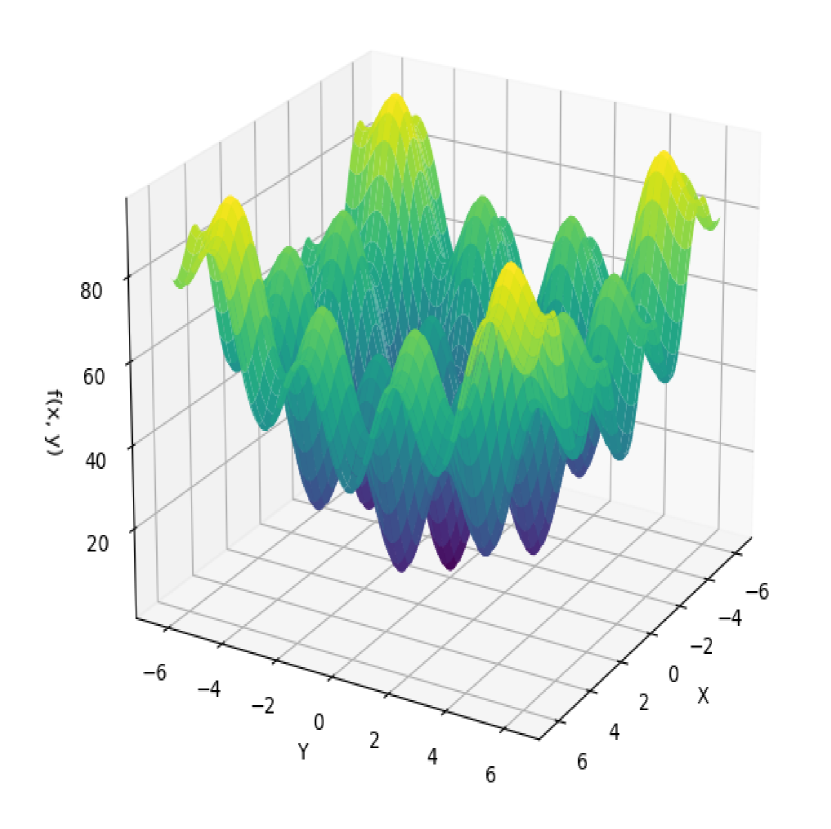
In order to evaluate the performance of our algorithm, we applied it to 6 standard benchmark functions. The function descriptions are detailed in Table 2.
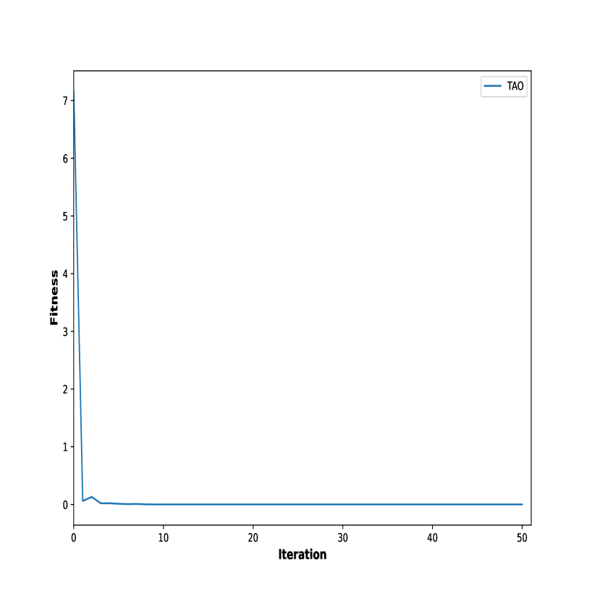
Given the stochastic nature of the meta-heuristic algorithms, their performance cannot be accurately assessed based on a single run. In order to evaluate the approach comprehensively, multiple trials with independently initialized populations are conducted. Consequently, TAO algorithm was run 50 times on each benchmark function, with a population size of 100 cells and maximum number of 500 iterations employed for both low- and high-dimensional problems.
| Function | Name | Dimension | Range | Minimum |
|---|---|---|---|---|
| Sphere | 20 | 0 | ||
| Rosenbrock | 10 | 0 | ||
| Eggcrate | 2 | 0 | ||
| Step | 30 | 0 | ||
| Rastrigin | 10 | 0 | ||
| Michalewicz | 5 | -4.6877… | ||
| Sum Squares | 30 | 0 |
In order to compare the performance of TAO algorithm we used standard PSO. Let’s remember that the PSO algorithm has the following equations to update the velocities and positions of the particles for each particle :
| (3) |
where and are, respectively, the velocity, position and personal best value of particle at time Furthermore, is the inertial weight, shows the individual coefficient, signifies the social coefficient, are random numbers uniformly distributed in is the global best, and shows the best solution found by all particles (entire swarm) until th iteration. Usually We used [39].
The inertia weight is inspired by the PSO algorithm and is calculated using the equation:
| (4) |
where is the current iteration step, is the maximum iteration step, is the maximum inertia weight, and is the minimum inertia weight. Usually, and [39, 44].
The initial velocities in the PSO algorithm are set to zero, as empirical evidence has shown this to be the most effective approach [12].
| Function | Parameters | PSO | TAO |
|---|---|---|---|
| Beast | 0.0416891 | 1e-07 | |
| Mean | 1.7180551 | 1.0434957 | |
| Standard deviation | 1.4389095 | 0.8459855 | |
| Beast | 2.7253815 | 0.0058221 | |
| Mean | 8.5999977 | 6.9607255 | |
| Standard deviation | 4.6557892 | 5.0302997 | |
| Beast | 0.0000000 | 0.0000000 | |
| Mean | 0.0000000 | 0.0000000 | |
| Standard deviation | 0.0000000 | 0.0000000 | |
| Beast | 0.306966 | 5.5e-06 | |
| Mean | 0.7906888 | 0.0010151 | |
| Standard deviation | 0.2765826 | 0.0015117 | |
| Beast | 1.6399746 | 0.9899181 | |
| Mean | 7.3307733 | 8.4788214 | |
| Standard deviation | 3.5371322 | 5.4759516 | |
| Beast | -4.8693888 | -4.6458954 | |
| Mean | 4.6169278 | -3.9887314 | |
| Standard deviation | 0.141926 | 0.5212977 | |
| Beast | 0.6684421 | 0.181605 | |
| Mean | 8.0236676 | 1.9926416 | |
| Standard deviation | 6.2222502 | 1.7023876 |
Statistical results of the performance of TAO and PSO algorithms on the benchmark problems presented in Table 3 indicate that the first algorithm outperforms the second in all cases.
4.2 Constrained optimization problems
Constrained optimization problems, encompassing both equality and inequality constraints, play a pivotal role in scientific and engineering disciplines, enabling the modeling of systems subject to physical laws, budget constraints, and operational requirements. Their applications span from structural design and resource allocation to parameter estimation and process optimization.
Optimization problems with constraints pose substantial challenges for metaheuristic algorithms. The complex nature of constraint handling necessitates innovative approaches.
Mathematically, constrained minimization problem are typically expressed as:
| (5) | ||||
| Subject to: | ||||
where are inequality constraints, are equality constraints, and are lower and upper bounds of and is the objective function that needs to be optimized subject to the constraints.
There exist five prominent constraint handling methodologies, which encompass: 1) penalty functions, 2) specialized representations and operators, 3) repair algorithms, 4) the separation of objectives and constraints, and 5) hybrid methods. Among these, penalty functions represent the most straightforward approach [9].
In this article, we employ TAO algorithm using the static penalty approach. Essentially, depending on the nature of the problem, as demonstrated in the application examples, we pursue two strategies. One strategy, the more natural approach, entails transforming problem (5) in the following problem:
| (6) | ||||
where functions and measure the extent to which the constraints are violated, and and are known as penalty parameters.
In the other strategy,
| (7) |
where is the number of constraints satisfied, is the total number of (equality and inequality) constraints and is a large constant () [29].
4.2.1 Rosenbrock function constrained with a cubic and a line
Let us first consider the problem of minimizing the Rosenbrock function subject to two inequality constraints: one is a cubic constraint, and the other is linear. This is a nonlinear constrained optimization problem with a global optimum at with
| (8) | ||||
| Subject to: | ||||
In order to solve problem (8), we rewrite it as follows:
| (9) |
where
TAO metaheuristic converges to the approximate solution with an absolute error
4.2.2 Cantilever Beam Design Problem
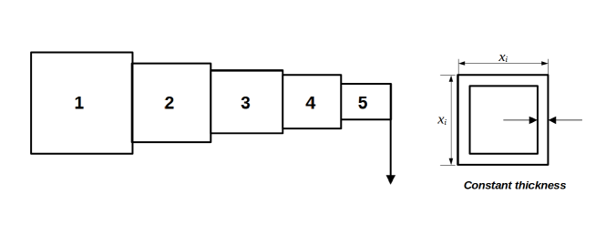
The Cantilever Beam Design Problem is a significant challenge in the fields of mechanics and civil engineering, primarily focused on minimizing the weight of a cantilever beam. In this problem, the beam consists of five hollow elements, each with a square cross-section. The goal is to determine the optimal dimensions of these elements while adhering to certain constraints (see figure 2).
The mathematical expression governing this problem and its associated constraints are represented by equation (10).
| (10) | ||||
| Subject to: | ||||
In order to address problem (10), we reformulate it as an unconstrained problem as follows:
| (11) |
where Subsequently, we apply TAO algorithm using a population of 100 individuals and a maximum of 300 iterations. Then, we obtain the approximate solution: with
Table 4 lists the best solutions obtained by TAO and various methods: artificial ecosystem-based optimization (AEO), ant lion optimizer (ALO), coot optimization algorithm (COOT), cuckoo search algorithm (CS), gray prediction evolution algorithm based on accelerated even (GPEAae), hunter-prey optimizer (HPO), interactive autodidactic school (IAS), multi-verse optimizer (MVO) and symbiotic organisms search (SOS) [31].
The comparative outcomes are presented within Table 4. These results clearly demonstrate that the TAO algorithm we propose presents a superior solution for addressing this problem.
| Algorithm | Optimum variables | Optimum weight | ||||
|---|---|---|---|---|---|---|
| TAO | 6.01601588 | 5.30917383 | 4.49432957 | 3.50147495 | 2.15266534 | 1.33652057 |
| AEO | 6.02885000 | 5.31652100 | 4.46264900 | 3.50845500 | 2.15776100 | 1.33996500 |
| ALO | 6.01812000 | 5.31142000 | 4.48836000 | 3.49751000 | 2.15832900 | 1.33995000 |
| COOT | 6.02743657 | 5.33857480 | 4.49048670 | 3.48343700 | 2.13459100 | 1.33657450 |
| CS | 6.0089000 | 5.30490000 | 4.50230000 | 3.50770000 | 2.15040000 | 1.33999000 |
| GPEAae | 6.0148080 | 5.30672400 | 4.49323200 | 3.50516800 | 2.15378100 | 1.33998200 |
| HPO | 6.00552336 | 5.30591367 | 4.49474956 | 3.51336235 | 2.15423400 | 1.33652825 |
| IAS | 5.9914000 | 5.30850000 | 4.51190000 | 3.50210000 | 2.16010000 | 1.34000000 |
| MVO | 6.0239402 | 5.30601120 | 4.49501130 | 3.49602200 | 2.15272610 | 1.33995950 |
| SOS | 6.0187800 | 5.30344000 | 4.49587000 | 3.49896000 | 2.15564000 | 1.33996000 |
4.2.3 Pressure vessel design problem
The aim of this problem is to achieve cost minimization encompassing material, forming, and welding expenses associated with a cylindrical vessel, as illustrated in Figure 3. The vessel is enclosed at both ends with a hemispherical-shaped head. There are four key variables in this problem: ( thickness of the shell), ( thickness of the head), ( inner radius) and ( length of the cylindrical section of the vessel, not including the head).
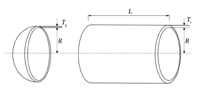
This problem is governed by four constraints. The formulation of these constraints and the problem is articulated as follows [19]:
| (12) | ||||
| Subject to: | ||||
To solve problem (12), we transform it into an unconstrained problem following strategy (7), with the number of constraints being TAO algorithm yields the following solution: with In accordance with the findings reported in the article [31], the comparative results with other algorithms are presented in Table 5. Algorithms under consideration include AEO, BA, charged system search (CSS), genetic algorithm (GA), GPEAae, Gaussian quantum-behaved particle swarm optimization (G-QPSO), GWO, Harris hawks optimizer (HHO), HPO, hybrid particle swarm optimization (HPSO), mothflame optimization (MFO), sine cosine gray wolf optimizer (SC-GWO), water evaporation optimization(WEO) and whale optimization algorithm (WOA). As inferred from the findings, the proposed TAO algorithm has demonstrated excellent performance in addressing this problem.
| Algorithm | Optimum variables | Optimum cost | |||
|---|---|---|---|---|---|
| TAO | 0.77873582 | 0.38572842 | 40.34900616 | 199.59130975 | 5888.6156573066 |
| AEO | 0.8374205 | 0.413937 | 43.389597 | 161.268592 | 5994.50695 |
| BA | 0.812500 | 0.437500 | 42.098445 | 176.636595 | 6059.7143 |
| CSS | 0.812500 | 0.437500 | 42.103624 | 176.572656 | 6059.0888 |
| GA | 0.812500 | 0.437500 | 42.097398 | 176.654050 | 6059.9463 |
| GPEAae | 0.812500 | 0.437500 | 42.098497 | 176.635954 | 6059.708025 |
| G-QPSO | 0.812500 | 0.437500 | 42.0984 | 176.6372 | 6059.7208 |
| GWO | 0.8125 | 0.4345 | 42.089181 | 176.758731 | 6051.5639 |
| HHO | 0.81758383 | 0.4072927 | 42.09174576 | 176.7196352 | 6000.46259 |
| HPO | 0.778168 | 0.384649 | 40.3196187 | 200 | 5885.33277 |
| HPSO | 0.812500 | 0.437500 | 42.0984 | 176.6366 | 6059.7143 |
| MFO | 0.8125 | 0.4375 | 42.098445 | 176.636596 | 6059.7143 |
| SC-GWO | 0.8125 | 0.4375 | 42.0984 | 176.63706 | 6059.7179 |
| WEO | 0.812500 | 0.437500 | 42.098444 | 176.636622 | 6059.71 |
| WOA | 0.812500 | 0.437500 | 42.0982699 | 176.638998 | 6059.7410 |
4.2.4 Tension/compression spring design problem
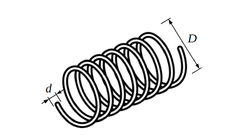
The engineering test problem employed in this study pertains to the optimization of tension/compression spring design. The objetive of this problem is to minimize the weight of a tension/compression spring associated with a spring characterized by three key parameters, namely the number of active loops (), the average coil diameter (), and the wire diameter (). The geometric details of the spring and its associated parameters are visually presented in Figure 4.
The spring design problem is governed by a set of inequality constraints, formally expressed in equation (13).
| (13) | ||||
| Subject to: | ||||
where and
To solve problem (13), we have applied the methodology described in approach (7), with the number of constraints in this problem being
| Algorithm | Optimum variables | Optimum weigth | ||
|---|---|---|---|---|
| TAO | 9.65579408 | 0.38821894 | 0.05296587 | 0.0126943602 |
| AEO | 10.879842 | 0.361751 | 0.051897 | 0.0126662 |
| BA | 11.2885 | 0.35673 | 0.05169 | 0.012665 |
| COOT | 11.34038 | 0.35584 | 0.05165 | 0.012665293 |
| CPSO | 11.244543 | 0.357644 | 0.051728 | 0.012674 |
| GPEAae | 11.294000 | 0.356631 | 0.051685 | 0.012665 |
| GWO | 11.28885 | 0.356737 | 0.05169 | 0.012666 |
| HHO | 11.138859 | 0.359305355 | 0.051796393 | 0.012665443 |
| HPO | 11.21536452893 | 0.3579796674 | 0.0517414615 | 0.012665282823723 |
| SFS | 11.288966 | 0.356717736 | 0.051689061 | 0.012665233 |
| SHO | 12.09550 | 0.343751 | 0.051144 | 0.012674000 |
| SSA | 12.004032 | 0.345215 | 0.051207 | 0.0126763 |
| WCA | 11.30041 | 0.356522 | 0.05168 | 0.012665 |
| WEO | 11.294103 | 0.356630 | 0.051685 | 0.012665 |
| WOA | 12.004032 | 0.345215 | 0.051207 | 0.0126763 |
Table 6 presents a comparative analysis of the results obtained using the TAO algorithm alongside other heuristic optimization methods in the context of this specific problem. This table provides comprehensive information concerning the values of each design variable and their respective optimization outcomes. Algorithms considered in the comparison of results are the following: AEO, BA, COOT, CPSO, GPEAae, GWO, HPO, HHO, stochastic fractal search (SFS), spotted hyena optimizer (SHO), salp swarm algorithm (SSA), water cycle algorithm (WCA), WEO and WOA. TAO algorithm produces the following solution: where
4.2.5 Sustainable exploitation of a natural renewable resource
In [16], a marine resource exploited from 1999 to 2019 is studied. It is assumed that the resource’s biomass, measured in tons, follows the Gordon-Schaefer equation, which is mathematically expressed as:
where represents the resource’s biomass in year , and are, respectively, the growth parameter and the carrying capacity of the fish population, and is the catch made in year . The catch is defined as where is the fishing effort, representing the intensity of human activities to extract fish, and is the catchability coefficient, representing the fraction of the population captured per unit of fishing effort. The unit of measurement for is boats-year (and, consequently, the unit of measurement for is 1/boats-year).
Using the Bayesian estimation MCMC method, the distributions of and were calculated based on empirical data [16]. The mean values of the estimated parameters are: Tn, and 1/boats-year. In 2019 (the initial time for our analysis), the biomass of the resource was Tn. Thus, we have the following model, with the estimated parameters, for the dynamics of the biomass of the resource subject to harvesting:
| (14) |
Now, we consider the problem of finding a harvesting strategy that allows for the exploitation of the fishery resource while maximizing the gains for the entity exploiting that resource. In other words, we seek strategies that maximize the catch benefits while simultaneously protecting the species over a time period where is known as the time horizon. To model the catch benefits, we can observe that if is the price per unit of fishing effort, then the profit at time is On the other hand, if is the unit cost per unit of fishing effort, then the losses at time are and the rent in year is given by Then, the benefit obtained years after 2019 is modeled as the following sum:
| (15) |
where
In order to protect the exploited species, strategies are sought to maximize its biomass at the final time i.e., the quantity Therefore, the objective is to maximize the following functional:
| (16) |
where is a discount factor chosen in
Interpretation of (16) is as follows: as time passes, less weight (or importance) is given to the benefit obtained by the entity that catches fish, and more weight is given to the protection of the resource, because, as increases, decreases. Furthermore, for biological reasons, it may be required that in each year, where and are minimum and maximum biomass threshold.
Thus, the following optimization problem is formulated:
| (17) | ||||
| Subject to: | ||||
where and are the minimum and maximum values of fishing effort.
| Parameter | Description | Value |
|---|---|---|
| Initial biomass | Tn | |
| Growth parameter | 0.7534 | |
| Carrying capacity | Tn | |
| Catchability coefficient | /boats-year | |
| Minimum fishing effort | 0 boats-year | |
| Maximum fishing effort | 41 boats-year | |
| Price per unit of fishing effort | $ 6 000 | |
| Unit cost per unit of fishing effort | $ 3 070 | |
| Time horizon | 30 | |
| Discount factor | ||
| Minimum biomass threshold | Tn | |
| Maximum biomass threshold | Tn |
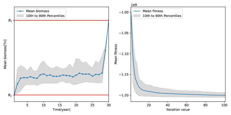
We used the parameters in Table 7 to conduct a 30-year sustainability study. For simplicity, instead of considering the interval , we have used the interval . We assume a scenario in which it is required that the biomass of the resource does not decrease below the initial biomass, that is, that of 2019. In addition, weight is assigned to the profits obtained, which leads us to consider a high value for , specifically, . To solve the optimization problem (17), we follow the strategy (6).
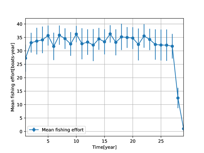
We realized 100 simulations, with population size of 50 cells and 100 iterations. The average biomass dynamics (see the right side of Figure 5) show that it is possible to exploit the resource sustainably, in the previously defined sense, with an average annual fishing effort such as that shown in Figure 6.
Various sustainability scenarios can be analyzed by considering different values of the parameter and different time horizons, For example, varying the value of allows us to assess the short, medium, and long-term impact of resource exploitation. Moreover, if is fixed, we can examine the impact of exploitation based on the emphasis placed on profits versus the preservation of the exploited resource.
5 Conclusiones
In this article, we present a new metaheuristic algorithm called Tumor Angiogenesis Optimizer (TAO). This algorithm is inspired by the morphogenetic cellular movements exhibited by ECs during the complex process of tumor angiogenesis. According to the results obtained from test functions, TAO outperforms the PSO standard. Furthermore, our algorithm has demonstrated high performance in real-world constrained optimization problems. In particular, in the context of cantilever beam design problems and pressure vessel design problems, it outperformed several well-established metaheuristics, while in the tension/compression spring design problem it had acceptable performance. In this article, we have also successfully addressed a sustainability problem related to the exploitation of a renewable resource.
For future work, the proposed algorithm can be used in different fields of study. In addition, we will delve into the mathematical modeling of the cellular angiogenesis process, focusing specifically on the phenomena of cell emergence and death, which could make the TAO algorithm more efficient. Furthermore, we aim to develop a version of our algorithm adapted to address multi-objective optimization problems.
References
- [1] Anderson, A. R., & Chaplain, M. A. (1998). Continuous and discrete mathematical models of tumor-induced angiogenesis. Bulletin of mathematical biology, 60(5), 857-899.
- [2] Arakelyan, L., Vainstein, V., & Agur, Z. (2002). A computer algorithm describing the process of vessel formation and maturation, and its use for predicting the effects of anti-angiogenic and anti-maturation therapy on vascular tumor growth. Angiogenesis, 5, 203-214.
- [3] Arima, S., Nishiyama, K., Ko, T., Arima, Y., Hakozaki, Y., Sugihara, K., … & Kurihara, H. (2011). Angiogenic morphogenesis driven by dynamic and heterogeneous collective endothelial cell movement. Development, 138(21), 4763-4776.
- [4] Arora, J. S. (2004). Introduction to optimum design. Elsevier.
- [5] Baish, J. W., Gazit, Y., Berk, D. A., Nozue, M., Baxter, L. T., & Jain, R. K. (1996). Role of tumor vascular architecture in nutrient and drug delivery: an invasion percolation-based network model. Microvascular research, 51(3), 327-346.
- [6] Bauer, A. L., Jackson, T. L., & Jiang, Y. (2009). Topography of extracellular matrix mediates vascular morphogenesis and migration speeds in angiogenesis. PLoS computational biology, 5(7), e1000445.
- [7] Bentley, K., Gerhardt, H., & Bates, P. A. (2008). Agent-based simulation of notch-mediated tip cell selection in angiogenic sprout initialisation. Journal of theoretical biology, 250(1), 25-36.
- [8] Chaplain, M. A., McDougall, S. R., & Anderson, A. R. A. (2006). Mathematical modeling of tumor-induced angiogenesis. Annu. Rev. Biomed. Eng., 8, 233-257.
- [9] Coello, C. A. C. (2002). Theoretical and numerical constraint-handling techniques used with evolutionary algorithms: a survey of the state of the art. Computer methods in applied mechanics and engineering, 191(11-12), 1245-1287.
- [10] Dey, N. (2023). Applied Genetic Algorithm and Its Variants: Case Studies and New Developments. Springer Nature.
- [11] Diwekar, U. M. (2020). Introduction to applied optimization (Vol. 22). Springer Nature.
- [12] Engelbrecht, A. (2012, June). Particle swarm optimization: Velocity initialization. In 2012 IEEE congress on evolutionary computation (pp. 1-8). IEEE.
- [13] Gilli, M., Maringer, D., & Schumann, E. (2019). Numerical methods and optimization in finance. Academic Press.
- [14] Goldengorin, B. (2016). Optimization and Its Applications in Control and Data Sciences. Springer.
- [15] Haupt, R. L., & Haupt, S. E. (2004). Practical genetic algorithms. John Wiley & Sons.
- [16] Hernández, M. (2022) Estrategias óptimas en modelos de explotación de recursos. Instituto Nacional de Investigación y Desarrollo Pesquero (INIDEP).
- [17] Hull, D. G. (2013). Optimal control theory for applications. Springer Science & Business Media.
- [18] Jakobsson, L., Franco, C. A., Bentley, K., Collins, R. T., Ponsioen, B., Aspalter, I. M., … & Gerhardt, H. (2010). Endothelial cells dynamically compete for the tip cell position during angiogenic sprouting. Nature cell biology, 12(10), 943-953.
- [19] Kannan, B. K., & Kramer, S. N. (1994). An augmented Lagrange multiplier based method for mixed integer discrete continuous optimization and its applications to mechanical design.
- [20] Keller, A. A. (2017). Mathematical optimization terminology: A comprehensive glossary of terms. Academic Press.
- [21] Kennedy, J., & Eberhart, R. (1995, November). Particle swarm optimization. In Proceedings of ICNN’95-international conference on neural networks (Vol. 4, pp. 1942-1948). IEEE.
- [22] Lenhart, S., & Workman, J. T. (2007). Optimal control applied to biological models. CRC press.
- [23] Lozovanu, D. (2009). Optimization and multiobjective control of time-discrete systems: dynamic networks and multilayered structures. Springer Science & Business Media.
- [24] Luptacik, M. (2010). Mathematical optimization and economic analysis (Vol. 287). New York: Springer.
- [25] Merks, R. M., Perryn, E. D., Shirinifard, A., & Glazier, J. A. (2008). Contact-inhibited chemotaxis in de novo and sprouting blood-vessel growth. PLoS computational biology, 4(9), e1000163.
- [26] Mirjalili, S., Mirjalili, S. M., & Lewis, A. (2014). Grey wolf optimizer. Advances in engineering software, 69, 46-61.
- [27] Mirjalili, S. (2019). Evolutionary algorithms and neural networks. In Studies in computational intelligence (Vol. 780). Berlin/Heidelberg, Germany: Springer.
- [28] Mirjalili, S., Dong, J. S., & Lewis, A. (2020). Nature-Inspired Optimizers Theories,
- [29] Morales, A. K., & Quezada, C. V. (1998). Literature Reviews and Applications. Springer Nature. A universal eclectic genetic algorithm for constrained optimization. In Proceedings of the 6th European congress on intelligent techniques and soft computing (Vol. 1, pp. 518-522).
- [30] Nanakorn, P., & Meesomklin, K. (2001). An adaptive penalty function in genetic algorithms for structural design optimization. Computers & Structures, 79(29-30), 2527-2539.
- [31] Naruei, I., Keynia, F., & Sabbagh Molahosseini, A. (2022). Hunter–prey optimization: Algorithm and applications. Soft Computing, 26(3), 1279-1314.
- [32] Oyelade, O. N., Ezugwu, A. E. S., Mohamed, T. I., & Abualigah, L. (2022). Ebola optimization search algorithm: A new nature-inspired metaheuristic optimization algorithm. IEEE Access, 10, 16150-16177.
- [33] Sethi, S. P., & Sethi, S. P. (2019). What is optimal control theory? Springer International Publishing.
- [34] Peirce, S. M. (2008). Computational and mathematical modeling of angiogenesis. Microcirculation, 15(8), 739-751.
- [35] Pettet, G. J., Byrne, H. M., McElwain, D. L. S., & Norbury, J. (1996). A model of wound-healing angiogenesis in soft tissue. Mathematical biosciences, 136(1), 35-63.
- [36] Rashedi, E., Nezamabadi-Pour, H., & Saryazdi, S. (2009). GSA: a gravitational search algorithm. Information sciences, 179(13), 2232-2248.
- [37] Scianna, M., Bell, C. G., & Preziosi, L. (2013). A review of mathematical models for the formation of vascular networks. Journal of theoretical biology, 333, 174-209.
- [38] Sugihara, K., Nishiyama, K., Fukuhara, S., Uemura, A., Arima, S., Kobayashi, R., … & Kurihara, H. (2015). Autonomy and non-autonomy of angiogenic cell movements revealed by experiment-driven mathematical modeling. Cell reports, 13(9), 1814-1827.
- [39] Shi, Y., & Eberhart, R. C. (1999, July). Empirical study of particle swarm optimization. In Proceedings of the 1999 congress on evolutionary computation-CEC99 (Cat. No. 99TH8406) (Vol. 3, pp. 1945-1950). IEEE.
- [40] Szabo, A., Mehes, E., Kosa, E., & Czirok, A. (2008). Multicellular sprouting in vitro. Biophysical journal, 95(6), 2702-2710.
- [41] Tyson, J. J. (2007). Bringing cartoons to life. Nature, 445(7130), 823-823.
- [42] Yang, X. S. (2008). Introduction to mathematical optimization: from linear programming to metaheuristics. Cambridge international science publishing.
- [43] Yang, X. S. (2010). A new metaheuristic bat-inspired algorithm. In Nature inspired cooperative strategies for optimization (NICSO 2010) (pp. 65-74). Berlin, Heidelberg: Springer Berlin Heidelberg.
- [44] Zhang, Y., Li, H., Bao, E., Zhang, L., & Yu, A. (2019). A hybrid global optimization algorithm based on particle swarm optimization and Gaussian process. International Journal of Computational Intelligence Systems, 12(2), 1270-1281.
- [45] Zolf, K. (2023). Gold rush optimizer: a new population-based metaheuristic algorithm. Operations Research and Decisions, 33(1).