We consider the problem of optimization of contributions of a financial planner such as a working individual towards a financial goal such as retirement. The objective of the planner is to find an optimal and feasible schedule of periodic installments to an investment portfolio set up towards the goal. Because portfolio returns are random, the practical version of the problem amounts to finding an optimal contribution scheme such that the goal is satisfied at a given confidence level. This paper suggests a semi-analytical approach to a continuous-time version of this problem based on a controlled backward Kolmogorov equation (BKE) which describes the tail probability of the terminal wealth given a contribution policy. The controlled BKE is solved semi-analytically by reducing it to a controlled Schrödinger equation and solving the latter using an algebraic method. Numerically, our approach amounts to finding semi-analytical solutions simultaneously for all values of control parameters on a small grid, and then using the standard two-dimensional spline interpolation to simultaneously represent all satisficing solutions of the original plan optimization problem. Rather than being a point in the space of control variables, satisficing solutions form continuous contour lines (efficient frontiers) in this space.

1 Introduction

We consider the problem of optimization of contributions of a financial planner such as a working individual towards a financial goal such as retirement. The objective of the planner is to find an optimal and feasible schedule of periodic installments to an investment portfolio set up towards the goal. Because portfolio returns are random, in practice this problem amounts to finding an optimal contribution scheme such that the goal is satisfied at a given confidence level. This problem is similar to the celebrated Merton (1971) optimal consumption problem [14], however it differs from the latter in at least three important aspects.

First, we do not address a portfolio optimization part of this problem, instead assuming that an investment portfolio set towards the goal has a fixed equity to cash ratio which is maintained by a financial fiduciary. This implies that a part of a regular cash contribution to the portfolio from the planner that is invested in equity is fixed by the fiduciary and is not subject to optimization.

Second, we do not maximize any utility of consumption, and respectively do not consider any consumption process either. Instead, we work directly with contributions to the financial plan as decision variables constrained by a net income, and our objective is to exceed a certain target wealth level at a terminal time $T$ at a given confidence level $\alpha$. In this sense, our problem formulation fits the setting of goal-based wealth management, see e.g. Das et. al. (2018) [4] and references therein.

The problem as formulated belongs in the class of optimal stochastic control problems, and thus could in principle be solved using conventional tools such as dynamic programming (DP) or reinforcement learning (RL). However, our problem is not necessarily a problem of adaptive (closed-loop) control type that are usually addressed with DP and RL methods. Retirement planning usually involves setting up a plan upfront, which is then revisited, if necessary, on the annual basis. A typical plan usually involves a time lime of annual installments, where annual contributions planned for the future are scheduled to increase to adjust for inflation, as well as possibly incorporate benefits from expected future increases in wages or other investable income. Such settings are typical for open-loop control problems, where an agent decides on the policy at the start, and then keeps it fixed for a certain fixed number of steps, without adapting it at each steps as is done in DP or RL.

Another important difference of our problem from the setting of DP or RL is that the latter methods solve a maximization problem for a value (or action-value) function. If the value function has a global maximum as a function of a deterministic policy, then there should be a policy - a point in a multi-dimensional action space whose position depends on the state - that attains this maximum. In contrast, a proper framework for decision-making in our setting is the framework of satisficing decision making of Herbert Simon (1955, 1979( [17, 18]. With this framework, we do not maximize an objective function. Instead, we only want to bring it to a certain goal level that we define beforehand. This involves two steps: search (i.e. exploring the objective function for different values of input controls), and satisficing (i.e. picking a solution that satisfies the goal criterion) [18]. Clearly, with this setting, feasible problems should in general produce continuous lines in the action space, rather than isolated points, as optimal solutions.

This paper suggests a semi-analytical solution to a continuous-time version of the problem formulated above. We use a probabilistic approach that amounts to analysis of two related equations. The first one is Fokker-Planck equation (FPE) whose solution is the probability density of the terminal wealth at the at time $T$, for a given contribution plan. The second equation is the backward Kolmogorov equation (BKE) which gives the probability of the terminal wealth to fall below a certain target wealth at a given confidence level $\alpha$. We solve the resulting controlled FPE and BKE equations semi-analytically by reducing them to controlled Schrödinger equations, and then solving the latter equations in a semi-closed form using an algebraic method. These semi-analytical solutions are computed simultaneously for all values of two control parameters describing annual contributions and their growth rate, on a small 2D grid of their discretized admissible values. Once the values of the tail BKE probability are computed for all nodes on the grid, its values for arbitrary inputs are cheaply obtained using the standard 2D cubic spline interpolation. This completes the search step of satisficing decision-making in our problem.

Once the search stage is completed, the satisficing part is rather simple, as all it takes is to draw constant-probability lines at the confidence levels $\alpha$ on the surface of the BKE tail probability function viewed as a function of initial controls. This task can be done using the standard 2D spline interpolation plus a root-finding algorithm, or equivalently using a contour-plotting algorithm that already combines the first two algorithms.

Therefore, in our approach, dubbed the Schrödinger Control Optimal Planning, or SCOP for short, the initial problem of contribution optimization amounts to the standard 2D spline interpolation plus a root-solving (or equivalently contour-plotting) algorithm, whose end result gives a visual representation of all possible satisficing plans at different confidence levels. Such visual representation is conceptualized via the notion of efficient frontiers: constant-level lines on the 2D surface of the BKE probability as the function of controls. This gives the planner the ability to perform a real time policy optimization for a given goal, or scenario analyses for different settings of the planning problem.

The paper is organized as follows. In Sect. 2, we present the theoretical framework for our problems. Sect. 3 describes our method for retirement plan optimization. Finally, a summary and an outlook for future research are presented in Sect. 4. All technical details and derivations are left to Appendices A, B, and C. The appendices have a hierarchical structure, i.e. Appendices B and C clarify certain technical details for topics discussed in Appendix A.

2 Optimal contribution problem

2.1 The investment portfolio dynamics

We consider a financial planner such as a retirement planner with a planning horizon $T$ who invests in a portfolio created towards a goal, expressed as a desired terminal wealth at time $T$. The investment portfolio has a fixed ratio $\omega$ of equity to the total portfolio value (e.g. $\omega=0.9$), which is assumed to be maintained by a fiduciary that manages the portfolio on client’s behalf.

Let $c_{t}\Delta t$ be the after-tax money flow from the planner to the portfolio in the time step $[t,t+\Delta t]$. This investment of cash from the planner forces the fiduciary to buy the amount of equity equal to $\omega c_{t}\Delta t$, which also incurs proportional transaction cost $\nu\omega|c_{t}|\Delta t$, where $\nu$ is a parameter. As we have $c_{t}\geq 0$ in our problem, in what follows we omit the absolute value expression in the transaction cost formula.

The investment portfolio is composed of cash $b_{t}$ and equity $s_{t}$. We assume that the cash infusion to the portfolio happens at time $t_{+}$ immediately after $t$, followed by an immediate purchase of equity by the fiduciary. The cash and equity positions at time $t_{+}$ are then obtained as follows:

$$b_{t}^{+} = b_{t}+\left((1-\omega)c_{t}-\nu\omega c_{t}\right)\Delta t$$

$$s_{t}^{+} = s_{t}+\omega c_{t}\Delta t$$ (1)

This produces the following update rule for the total portfolio value $\Pi_{t}:=b_{t}+s_{t}$:

$$\Pi_{t}^{+}=\Pi_{t}+\left(c_{t}-\nu\omega c_{t}\right)\Delta t$$ (2)

We assume that equity has random returns

$$r_{e}(t)=\hat{r}_{e}+\frac{\hat{\sigma}_{e}}{\sqrt{\Delta t}}\xi_{t},\;\;\;\xi_{t}\sim\mathcal{N}(0,1)$$ (3)

with a mean value $\hat{r}_{e}$, while the cash component has a deterministic return $r_{f}$. Using the fact that $s_{t}=\omega V_{t}$ and taking the continuous-time limit $\Delta t=dt\rightarrow 0$, we obtain a stochastic differential equation (SDE) for the portfolio value $V_{t}$:

$$d\Pi_{t}=\left(\bar{r}\Pi_{t}+u_{t}\right)dt+\sigma\Pi_{t}dW_{t}$$ (4)

here $W_{t}$ is a standard Brownian motion, and the decision variable $u_{t}$ and parameters $\bar{r},\sigma$ are defined as follows:

$$u_{t}:=(1-\nu\omega)c_{t},\;\;\;\bar{r}:=r_{f}+\omega(\hat{r}_{e}-r_{f}),\;\;\;\sigma:=\omega\hat{\sigma}_{e}$$ (5)

In this paper, we consider contribution policies parameterized in terms of an initial contribution rate $u_{0}$ and a growth rate $\xi$:

$$u_{t}=u_{0}e^{\xi t}$$ (6)

so that $u_{0}$ and $\xi$ are now the constrained decision variables for the planner. The growth rate $\xi$ can be tuned to compensate for inflation or increase future contributions, assuming that the net investable income will grow in the future.

2.2 Stochastic Verhulst equation and Langevin dynamics

Note that Eq.(4) is a controlled SDE where control variables are $u_{0}$ and $\xi$. To simplify these dynamics, we introduce a new dimensionless variable $v_{t}$ defined as follows:

$$v_{t}=\frac{2}{\sigma^{2}}\frac{u_{t}}{\Pi_{t}}=\frac{2}{\sigma^{2}}\frac{u_{0}e^{\xi t}}{\Pi_{t}},\;\;\;$$ (7)

Note that the new variable $v_{t}$ blends together the state variable $\Pi_{t}$ and action variable $u_{t}$. Using Itô’s lemma, we obtain the SDE for $v_{t}$:

$$dv_{t}=v_{t}\left(\xi-\bar{r}+\sigma^{2}-\frac{\sigma^{2}}{2}v_{t}\right)dt+\sigma v_{t}dW_{t}$$ (8)

The new SDE for $s_{t}$ does not depend on $u_{0}$, which is now embedded into the problem via the initial value $v_{0}$. The only remaining control parameter explicitly appearing in (8) is $\xi$.

The SDE (8) is known in the literature as the stochastic Verhulst equation, see e.g. Giet et. al. (2015) [6]. Recently, the SDE (8) with time-dependent coefficients was proposed by Itkin, Lipton and Muravey (2020) [10] as an attractive model of short interest rates that addresses some deficiencies of the classical Black-Karasinski model. Furthermore, they developed a method of solving the BKE for the SDE (8) with general time-dependent coefficients using an original integral transform method [11]. The method of Itkin, Lipton and Muravey (2020) [10] could be considered as an alternative approach to the semi-analytical method developed in this paper, see also the summary section for further comments.

To transform the multiplicative noise in the resulting SDE into an additive noise, we apply one more transformation to a new variable $x_{t}$:

$$x_{t}=-\log v_{t}$$ (9)

so that $v_{t}=e^{-x_{t}}$. The SDE for $x_{t}$ reads

$$dx_{t}=-\left(\eta-\frac{\sigma^{2}}{2}e^{-x}\right)dt+\sigma dW_{t},\;\;\;\eta:=\xi-\bar{r}+\frac{\sigma^{2}}{2}$$ (10)

The new parameter $\eta$ introduced in the SDE (10) can be used as a new control variable in liew of $\xi$, with constraints inherited from constraints on $\xi$.

Now, the SDE (10) can be viewed as an (overdamped) Langevin equation

$$dx_{t}=-\frac{\partial V}{\partial x_{t}}dt+\sigma dW_{t}$$ (11)

where the potential function $V=V(x)$ is defined as follows:

$$V(x)=\eta x+\frac{\sigma^{2}}{2}e^{-x}$$ (12)

so that $\eta$ becomes a control parameter for the Langevin potential $V(x)$.

Consider now the conditional tail probability $p(w,t):=P^{(\pi)}[\Pi_{T}<\hat{\Pi}|\Pi_{t}=w]$, where $\Pi_{T}$ stands for the terminal wealth at time $T$, $\hat{\Pi}$ is a target wealth, and the notation $P^{(\pi)}\left[\cdots\right]$ is introduced to emphasize the dependence of this conditional probability on the policy $\pi:=(u_{0},\xi)$. Our problem amounts to the task of choosing optimal values of $u_{0}$ and $\xi$ such that the conditional tail probability $p(v,0)$ as seen now at time $t=0$ does not exceed a certain target probability level $\alpha$ such as $\alpha=5\%$. Now, when conditioning on the policy $\pi:=(u_{0},\xi)$, we can equivalently compute the tail probability $p(v,t)$ in terms of variables $v_{t}$ and $x_{t}$ introduced above. Denoting corresponding target variables computed according to Eqs.(7) and (9) as $\hat{v}$ and $\hat{x}$, we can write down the following chain of equations:

$$P^{(\pi)}\left[\Pi_{T}\leq\hat{\Pi}|\Pi_{t}=w\right]=P^{(\pi)}\left[v_{T}\geq\hat{v}|v_{t}=v\right]=P^{(\pi)}\left[x_{T}\leq\hat{x}|x_{t}=x\right]$$ (13)

This shows that the tail probability $P^{(\pi)}\left[\Pi_{T}\leq\hat{\Pi}|\Pi_{t}=w\right]$ of the original problem can be equivalently computed using the variable $x_{t}$. As will be shown next, the advantage of doing this is that using the variable $x_{t}$, our problem has a semi-analytical solution.

2.3 From the Fokker-Planck-Kolmogorov control to the Schrödinger control

The Langevin dynamics expressed by Eq.(11) have an equivalent probabilistic formulation in terms of the corresponding Fokker-Planck equation (FPE) for the probability density $f(x,t)$:

$$\frac{\partial f(x,t)}{\partial t}=\frac{\partial}{\partial x}\left[\frac{\partial V}{\partial x}f(x,t)\right]+\frac{\sigma^{2}}{2}\frac{\partial^{2}f(x,t)}{\partial x^{2}}$$ (14)

The probability density $f(x,t)$ that solves the FPE equation is a distribution of $x_{t}$ at time $t$ given controls $(u_{0},\eta)$. To ease the notation, the dependence on controls is suppressed in all relations in this section.

The second probability function we consider is the tail probability $p(x,t):=P^{(\pi)}\left[x_{T}\leq\hat{x}|x_{t}=x\right]$. It satisfies the backward Kolmogorov equation (BKE):

$$\frac{\partial p}{\partial t}-\frac{\partial V}{\partial x}\frac{\partial p}{\partial x}+\frac{\sigma^{2}}{2}\frac{\partial^{2}p}{\partial x^{2}}=0$$ (15)

with the terminal condition

$$p(x,T)=\theta\left(\hat{x}-x\right),\;\;\;\hat{x}:=\log\frac{\hbar\hat{\Pi}}{2u_{0}e^{\xi T}}$$ (16)

Let us look for solutions of the FPE (14) and BKE (15) in the following form:

$$f(x,t) = e^{-\frac{V(x)}{\hbar}}\Psi(x,t),\;\;\;\hbar:=\sigma^{2}$$ (17)

$$p(x,t) = e^{\frac{V(x)}{\hbar}}\bar{\Psi}(x,\tau),\;\;\;\tau:=T-t$$

Here we introduced a new parameter $\hbar=\sigma^{2}$ to make formulae to follow look more familiar. Also note the time reversal $t\rightarrow\tau=T-t$ in the second relation.

Substituting these expressions back into Eqs.(14) and (15), we obtain a pair of PDEs for $\Psi(z,t)$ and $\bar{\Psi}(z,\tau)$:

$$-\hbar\frac{\partial\Psi(x,t)}{\partial t}=\left[-\frac{\hbar^{2}}{2}\frac{\partial^{2}}{\partial x^{2}}+U(x)\right]\Psi(x,t)$$ (18)

$$-\hbar\frac{\partial\bar{\Psi}(x,\tau)}{\partial\tau}=\left[-\frac{\hbar^{2}}{2}\frac{\partial^{2}}{\partial x^{2}}+U(x)\right]\bar{\Psi}(x,\tau)$$ (19)

where

$$U(x)=\frac{1}{2}\left(\frac{\partial V}{\partial x}\right)^{2}-\frac{\hbar}{2}\frac{\partial^{2}V}{\partial x^{2}}$$ (20)

Written in this form, Eqs.(18) and (19) should look very familiar to the reader acquainted with quantum mechanics. Eq.(18), formulated in time $t$, is the Schrödinger equation in Euclidean (imaginary) time with the ’Planck constant’ $\hbar=\sigma^{2}$ and potential $U(x)$. On the other hand, Eq.((19) is the Schrödinger equation in backward time $\tau=T-t$. In what follows, we will refer to Eqs.(18) and (19) as, respectively, the Fokker-Plack Schrödinger equation (FP-SE), and the backward Kolmogorov Schrödinger equation (BK-SE).

Note that while the FP-SE (18) and BK-SE (19) have identical forms, they satisfy different initial conditions:

$$\Psi(x,0)=e^{\frac{V(x)}{\hbar}}\delta\left(x-x_{0}\right),\;\;\;\;\bar{\Psi}(x,0)=e^{-\frac{V(x)}{\hbar}}\theta\left(\hat{x}-x\right)$$ (21)

This implies that $e^{-\frac{V(x)}{\hbar}}\Psi(x,t)$ is the Green’s function for Eq.(19), and therefore, we can relate the two functions as follows:

$$\bar{\Psi}(x,T)=\int_{-\infty}^{\infty}dx^{\prime}e^{-\frac{V(x^{\prime})}{\hbar}}\bar{\Psi}(x^{\prime},0)\Psi(x,T|x^{\prime},0)$$ (22)

Using Eq.(17), this relation is seen to be equivalent to the conventional Feynman-Kac expression for the tail probability $p(x,0)$:

$$p(x,0)=e^{\frac{2V(x)}{\hbar}}\int_{-\infty}^{\infty}dx^{\prime}e^{-\frac{2V(x^{\prime})}{\hbar}}\theta(\hat{x}-x^{\prime})f(x,T|x^{\prime},0)$$ (23)

While the Feynman-Kac formula (23) gives one representation of a solution to our problem, an alternative approach is to directly solve the SE (19) with the initial condition stated in (21). As Eqs.(18) and (19) have the same Hamiltonian, their solutions can be found by expanding in the same set of basis functions. Therefore, it might be more convenient to directly solve the the BK-SE (19) because it does not involve an extra integration step of the Feynman-Kac representation (23), at least formally.

2.4 The Morse potential

The Schrödinger potential (20) for our problem is obtained using Eq.(12):

$$U(x)=D_{0}\left(1-\frac{1}{g}e^{-x}\right)^{2}+U_{0}$$ (24)

where we defined the following parameters:

$$g:=1+\frac{2\eta}{\hbar}=2\left(1+\frac{\xi-\bar{r}}{\hbar}\right),\;\;\;D_{0}:=\frac{\hbar^{2}}{8}g^{2},\;\;\;U_{0}:=-\frac{\hbar^{2}}{8}(2g-1)$$ (25)

The control variable $\xi$ of the original problem is now embedded into the ’coupling constant’ parameter $g$ of the corresponding quantum mechanical problem (18) or (19). The original control problem therefore becomes a problem of quantum control for the Euclidean quantum mechanics. In this problem, we control the coupling constant $g$ of the quantum mechanical potential $U(x)$ and the initial position of a quantum mechanical ’particle’ representing the wealth of the planner in such a way that the terminal WF $\bar{\Psi}(x,T)$ is driven to a desired form.

In its turn, the coupling constant $g$ determines the degree of non-linearity of potential $U(x)$. If $g>0$, the potential has a minimum at $x=-\log g$. In the limit $g\rightarrow 0$, the minimum is pushed to infinity, and we obtain $U(x)=(\hbar^{2}/8)\left(1+e^{-2x}\right)$, i.e. the potential becomes a monotonically decreasing function. In the opposite limit $g\rightarrow\infty$, the potential $U(x)$ becomes a constant $U(x)=D_{0}+U_{0}$. For $g<0$, the potential $U(z)$ has no minima or maxima, and becomes a monotonically decreasing function.

The potential $U(x)$ can be written more compactly once we differentiate between two possible regimes $g>0$ and $g<0$ of the model. Introducing parameter $x_{\star}:=-\log|g|$, we can write the potential $U(x)$ in the following form:

$$U(x)=\left\{\begin{array}[]{l}D_{0}\left(1-e^{-(x-x_{\star})}\right)^{2}+U_{0},\;\;\;\text{if}\;\;\;g>0\\ D_{0}\left(1+e^{-(x-x_{\star})}\right)^{2}+U_{0},\;\;\;\text{if}\;\;\;g<0\\ \end{array}\right.$$ (26)

Focusing on the first expression here obtained for $g>0$, this is the celebrated Morse potential known from quantum mechanics, see Landau (1980) [12], see Fig.1. As this potential is very tractable, the reduction of our initial financial problem to Schrödinger equations (18), (19) with the Morse potential $U(x)$ is very helpful. More specifically, it enables semi-analytical solutions for both Schrödinger equations (18) and (19), and hence for both the FPE (14) and BKE (15) by virtue of Eq.(17). We only give here the final expressions for the FPE and BKE solutions $f(x,t)$ and $p(x,t)$. Details are left to Appendix A which is written in a reasonably self-contained way to provide a brief overview of these methods for the reader without a background in theoretical physics.

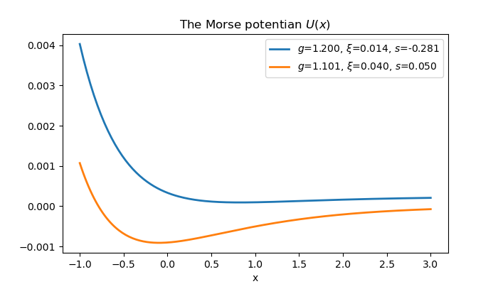
Figure 1: Examples of the Morse potential for different values of parameter $g$ driven by different values of control parameter $\xi$. Both potentials have a minimum at $x_{\star}=-\log(g)$ where $g=2s+1$. For small values of $\xi$, the potential well becomes very shallow. If $\xi$ becomes smaller than $\xi_{low}:=\bar{r}-\sigma^{2}$, the minimum disappears, and the potential becomes monotonically decreasing. For larger values of $\xi$, the minimum becomes more pronounced.

The solution presented in Appendix A shows that both functions $\Psi(x,t)$ and $\bar{\Psi}(x,t)$ depend on $x$ only through the so-called Morse variable $y:=e^{-x}$, so that we can equivalently write them as $\Psi(y,t),\,\bar{\Psi}(y,t)$. Recalling Eq.(9), the time-$t$ Morse variable value $y_{t}$ can be expressed in terms of the original model inputs:

$$y_{t}=e^{-x_{t}}=\frac{2u_{0}e^{\xi t}}{\hbar\Pi_{t}}$$ (27)

If we use this relation for $t=0$, it means that the initial value $y_{0}$ at time zero is simply the initial contribution $u_{0}$ scaled by the portfolio value $\Pi_{0}$ and portfolio variance $\hbar=\sigma^{2}$. In other words, $y_{0}$ can be viewed as a correct dimensionless version of the initial control $u_{0}$ (which has the dimension of dollars per year) which enables a meaningful comparison of different plans and different market conditions. For this reason, in most of our numerical examples to follow we will use the initial value $y_{0}$ of the Morse variable as a dimensionless control parameter in lieu of the initial control parameter $u_{0}$.

As $\Psi(x,t),\,\bar{\Psi}(x,t)$ are functions of the Morse variable $y$, it is convenient to reformulate Eqs.(17) in terms of the Morse variable $y=e^{-x}$. For the exponential factor $e^{-V(x)/\hbar}$, it gives

$$e^{-V(y)/\hbar}=\left.e^{-V(x)/\hbar}\right|_{x=-\log y}=y^{\eta/\hbar}e^{-y/2}$$ (28)

Changing the variables in Eq.(17) to the Morse variable $y=e^{-x}$, we write them as follows

$$f(y,t) = y^{-1}e^{-V(y)/\hbar}\Psi(y,t)=y^{\eta/\hbar-1}e^{-y/2}\Psi(y,t)$$ (29)

$$p(y,t) = e^{V(y)/\hbar}\bar{\Psi}(y,\tau)=y^{-\eta/\hbar}e^{y/2}\bar{\Psi}(y,\tau)$$

The explicit form of the FP-SE WF $\Psi(y,t)$ and the BK-SE WF $\bar{\Psi}(y,t)$ is given in Eqs.(A.51) and (A.52), respectively.

In Fig. 2, we show 3D views of the WF $\bar{\Psi}(y,T)$ and the BKE density $p(y,0)$ as a function of two variables $y=y_{0}$ and $\xi$ for a typical retirement plan with the horizon $T=20Y$ for the target wealth of $2.5m, initial wealth of $0.5m, and portfolio volatility of 30%, with the following bounds on admissible values of $u_{0}$ and $\xi$: $10k $\leq u_{0}\leq$ $100K, and $2.5\%\leq\xi\leq 5.0\%$. This parameter and constraints settings will also be used below in other examples illustrating the working of the model.

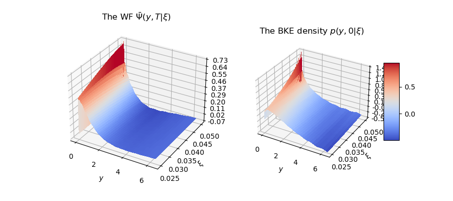
Figure 2: On the left: The WF $\bar{\Psi}(y,T)$ for $T=20$, shown as a function of both $y$ and $\xi$ using $N=150$ basis functions, for a retirement plan with the horizon $T=20Y$, the target wealth of $2.5m, the initial wealth of $0.5m, and portfolio volatility of 30%, with the following bounds on admissible values of $u_{0}$ and $\xi$: $10k $\leq u_{0}\leq$ $100K, and $2.5\%\leq\xi\leq 5.0\%$. On the right: the corresponding BKE tail probability $p(y,0)$.

Note that using Eqs.(29), we can obtain the Chapman-Kolmogorov equation in terms of $\Psi(x,t)$ and $\bar{\Psi}(x,t)$:

$$\int p(x,t)f(x,t|x_{0},t_{0})dx=\int\Psi(x,t)\bar{\Psi}(x,t)dx=P\left[\left.x_{T}\leq\hat{x}\right|x_{0},t_{0}\right]$$ (30)

which resembles the normalization condition $\int\left|\Psi(x,t)\right|^{2}dx=1$ in quantum mechanics.

3 Optimization of contribution policy: efficient frontiers

Optimization of contribution policy is performed using the semi-analytical solution given by the second equation in Eqs.(29) which gives the tail probability of the event $\Pi_{T}<\hat{\Pi}$ in terms of the tail probability of the Morse variable $y$:

$$P\left[\left.\Pi_{T}\leq\hat{\Pi}\right|\Pi_{t},u_{t}\right]=P\left[y_{T}\geq\hat{y}|y_{t},\xi\right]=y^{-\eta/\hbar}e^{y/2}\bar{\Psi}(y,t|\xi)$$ (31)

Here $\hat{y}$ is the target value of the Morse variable $y$, which is computed according to Eq.(27):

$$\hat{y}=\frac{2u_{0}e^{\xi T}}{\hbar\hat{\Pi}}$$ (32)

and we wrote the WF $\bar{\Psi}(y,t)$ as $\bar{\Psi}(y,t|\xi)$ to emphasize its dependence on $\xi$.

Our strategy for optimization of contribution policy is to compute Eq.(31) for all possible values of control variables $u_{0}$ and $\xi$, and then find the optimal control that matches the threshold value for the BKE tail probability $p(y,0)$. In practice, this involves computing the tail probability (31) for all nodes of a certain two-dimensional grid for $u_{0}$ and $\xi$, and then interpolating to other values of $u_{0}$, $\xi$ using splines. As in the range of input parameter that have practical interest the model behaves in a very smooth way (see Fig. 2), this means that we can use a rather small grid of pairs $(u_{0},\xi)$ to perform accurate spline interpolation.

Furthermore, the mathematical structure of the solution to our problem suggests that instead of considering the pair $(u_{0},\xi)$ as independent controls, we can equivalently but more conveniently map them onto the pair $(y,\xi)$. As suggested by Eq.(27), $y$ is the right dimensionless version of $u_{0}$, additionally scaled by the portfolio volatility, therefore using variable $y$ instead of the absolute dollar amount $u_{0}$ enables comparing different plans and different market conditions. If the current time is set to zero and the initial wealth $\Pi_{0}$ is fixed, then values of $u_{0}$ corresponding to values of $y=y_{0}$ are obtained according to (27):

$$u_{0}=\frac{\hbar}{2}y_{0}\Pi_{0}$$ (33)

In our numerical examples presented below, we use a non-uniform grid of values of $y$ of size 100. In addition, we use 20 grid points to represent possible values of $\xi$. The values of the BKE density for arbitrary intermediate inputs are obtained using the standard 2D cubic splines.

As the inputs $(\xi,y)$ (or equivalently $(\xi,u_{0})$) form a 2D plane, Eq.(31) implies that the problem of finding the optimal contributions $u^{\star}=(u_{0}^{\star},\xi^{\star})$ for a plan with the goal wealth $\hat{\Pi}$ that we want to exceed with probability equal to $1-\alpha$ amounts to solving the equation

$$P\left[y_{T}>\hat{y}|y_{t},\xi_{t},t\right]=\alpha$$ (34)

in this 2D $(\xi y)$-plane.

Note that we call here an optimal solution $u^{\star}=(u_{0}^{\star},\xi^{\star})$ is in fact a satisficing solution: we do not want to drive the tail probability (34) all the way down to zero, we only need to drive it below the target confidence level $\alpha$. Satisficing decision-making is different from decision-making based on maximization of a total reward as is done in DP or RL. Indeed, with DP or RL, a reasonably-behaved value function should have a global maximum, therefore there should be at least one policy that leads to such maximum value. Quite differently, with satisficing decision-making problems such as our Eq.(34), solutions for feasible problems form contour lines on the surface of BKE density $p(y,0|\xi)$.

We will refer to such contour lines at different probability levels as efficient frontiers, similarly to the use of this term in the Markowitz (1956) portfolio theory [13]. The 3D plot of the BKE tail probability $p(y,0|\xi)$ as a function of both controls $y$ and $\xi$ with efficient frontier lines is shown in Fig. 3. The corresponding 2D view that might be easier for analysis is shown in Fig. 4.

Efficient frontier lines shown in Figs. 3 and 4 can be used for visualization of all possible optimal policies at different confidence levels $\alpha$ for a given plan with user-defined initial and target wealth levels and constraints on admissible values of control parameters. Note that while our original objective was formulated as an optimization problem, the solution presented here reduces to a combination of a 2D cubic spline and a root-finding, or equivalently a contour construction algorithm. The plan optimization part thus reduces to the task of drawing a constant-probability line on a computed solution surface given by the BKE density $p(y,t|\xi)$.

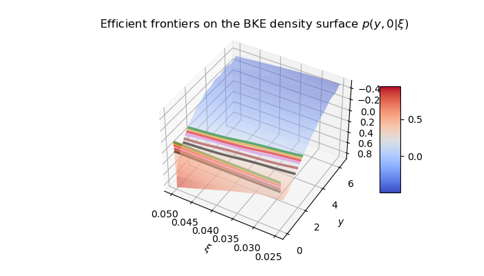
Figure 3: 3D plot of the BKE tail probability $p(y,0|\xi)$ viewed as a function of both control variables $y$ and $\xi$, along with efficient frontier lines corresponding to probability confidence levels $\alpha=[3,5,7.5,10,15,20]\%$.

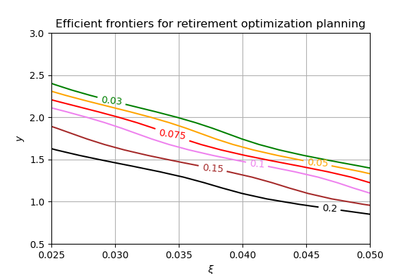
Figure 4: The 2D view of efficient frontier lines in the 3D space in Fig. 3. Lines in the $(\xi y)$-plane labeled by numbers and colors are efficient frontiers of the planning problem at the confidence levels $\alpha$ marked on the curve. For any fixed value of $\alpha$, any point on a line is as good as any other point in terms of the quality of the solution obtained with the model. Further preferences may be based on other considerations that were not used as a part of model inputs.

4 Summary

This paper addresses a problem that is routinely solved (or at least supposed to be routinely solved) by millions of working individuals who participate in retirement saving plans such as the 401(K) plans in the US, or similar programs worldwide. The problem is to plan an optimal contribution schedule to their investment portfolio so that their wealth by the time of retirement will be above a certain target wealth level at a certain probability confidence level.

While his problem appears to be entirely unrelated to any sort of quantum physics, what we proposed in this paper is that in fact, this problem is quantum mechanics in disguise! This of course does not mean quantization of the retirement wealth, or (unfortunately!) a teleportation to a wealthier quantum state, or anything of this sort that can come to the minds of non-physicists when they hear the words ’quantum mechanics’ or ’Schrödinger equation’. What we mean by saying “retirement planning is quantum mechanics in disguise” rather refers to the fact that, with standard simplifications and assumptions of normal equity returns etc., the first problem is mathematically identical to a very famous problem in quantum mechanics, namely quantum mechanics with the Morse potential.

It is interesting to note here that the non-linear Morse potential (26) arises in our approach due to the mere presence of controls $(u_{0},\xi)$. Indeed, if we take $u_{t}=0$ in Eq.(4), we end up with the standard Geometric Brownian Motion (GBM) model as a model of the portfolio wealth process. This can be contrasted with scenarios where the uncontrolled dynamics are non-linear due to a non-linear potential. Models of non-linear dynamics for equity stock markets with nonlinearity generated by market flows and market frictions have been previously proposed by the author in (Halperin, 2021, 2022 [8, 9].) In contrast, in this paper we start with linear uncontrolled dynamics of the GBM model, while non-linearities arise in the mathematically equivalent formulation of the problem based on a transition to the Morse variable $y$ that blends together the state and action variables.

Our method can be compared with the conventional feedback-loop control approach of dynamic programming (DP) or reinforcement learning (RL). It is well known that low dimensional problems with continuous controls can be efficiently solved by discretization of action variables. Therefore, the mere fact of reducing our 2D control problem to a 2D grid search problem may be hardly surprising on its own. Nonetheless, for practical applications that we have in mind for this paper, the end criteria of success are the accuracy and the speed of calculation. The approach of this paper can be viewed as a way to efficiently construct a grid of policies and value functions (i.e. BKE tail probabilities, in our case) using methods that work in physics.

While our step of constructing a grid of controls and output BKE tail probabilities is similar to the procedure employed in DP and RL upon discretization of action variable, one important difference of our scheme from DP or RL is what we do next with this grid. With DP or RL, we want to find a policy (i.e. a grid point) where the value function attains its global maximum - which can be performed via a regular grid search because of discretization. In contrast, with goal-based wealth management, our setting fits the framework of satisficing decision-making of Herbert Simon (1955, 1979) [17, 18]. This is because with goal-based wealth management, we want to find a policy that is good enough (i.e. satisficing) to drive the probability of the terminal portfolio wealth falling below some target value $\hat{\Pi}$ to the level of $\alpha$, but not below! This is not a maximization problem that is usually solved by DP or RL, this is a problem of finding contour lines on a surface of the BKE tail probability. Therefore, the nature of a solution for DP or RL is quite different from a solution to satisficing decision making: while the solution is given by a point in an action space for the former, it has a form of a degenerate contour line for the latter.

One important concept that we propose here as a way to communicate the model results to end users is the notion of efficient frontiers - constant probability level curves on the surface of the BKE tail probability $p(y,0|\xi)$ viewed as a function of control parameters $y$ and $\xi$. Note here that most of RL methods typically provide a single point in a multi-dimensional action space as an optimal solution to a stochastic control problem. While the present paper emphasizes the importance of continuous degenerate families of solutions (efficient frontiers) for our particular 2D control problem with a satisficing objective function, the author is unaware of any systematic discussion of degenerate satisficing solutions in a general RL setting.

Back to the mathematical identity of the retirement planning problem to the quantum mechanical problem, note that we reduced our initial problem not just to the standard textbook problem of solving the Schrödinger equation with a fixed Morse potential, but rather to a quantum optimal control problem with the Morse potential. Unlike the passive dynamics problem of the conventional quantum mechanics, in tasks of quantum control, the objective is to control the Schrödinger potential in order to bring a quantum system into a desired terminal state at a smallest cost or in a shortest time. In the same way, here we control the degree of non-linearity of the Morse potential and the initial particle position in order to achieve a desired quantum mechanical terminal state $\bar{\Psi}(y,T)$. In this sense, the proposition formulated in the beginning of this section can be refined to the following proposition:

The wealth management problem is a quantum optimal control problem in disguise.

where, as before, by saying in disguise we mean mathematically equivalent. A recent work applied quantum computing to quantum mechanics of molecules with the Morse potential to compute energies of two lowest eigenstates by Apanasevich et. al. (2021) [2]. Exploring potential applications of quantum computing to the problem formulated in this paper and its potential extensions can be an interesting venue for future research.

Another interesting direction would be to explore alternative methods for the FPE and BKE equations which may or may not make connections to the Schrödinger equation as we did in this paper. While here we solved the BKE equation and its associated Schrodinger equation using the standard eigenvalue decomposition method coupled with a non-standard way of constructing the basis, this is clearly not the only available, and likely not the most efficient way to solve these equations. In particular, it would be interesting to apply the integral transform approach of Ref. [10] in our setting of optimal control. Finally, extensions to multiple dimensions can be another interesting topic for future research along the lines proposed in this paper.

Appendix A: Schrödinger equation with the Morse potential

In this appendix, we provide semi-analytical solutions for both Schrödinger equations (18) and (19) which we referred to in the main text as FP-SE and BK-SE, respectively. As both SEs share the same Hamiltonian and only differ in the initial conditions, solutions for both equations will be found using a variant of the eigenvalue decomposition method, where the only difference between Eqs.(18) and (19) amounts to different initial conditions. We will start our analysis with the FP-SE (18) and then shown where the final formulae for the BK-SE (19) differ from the final formulae for the FP-SE (18).

Our approach largely follows Ref.[16] that offers a semi-analytical approach to the time-dependent SE with the Morse potential using the standard basis function decomposition method for PDEs. The novelty of this method is in the way of constructing the basis itself. The method of [16] gives rise to a ’natural’ infinite and countable basis for the Hilbert space corresponding to the SE (18).

The method of [16] is based on a recursive algebraic procedure which is rooted in supersymmetric quantum mechanics (SUSY QM) of Witten [20], see e.g. [3] for a review. To ensure that the present paper is reasonably self-contained and can be read by a diverse audience that does not only include theoretical physicists, this appendix provides a short overview of this approach, together with its application to our problem.

We start with Eqs.(17) which we repeat here for convenience:

$$f(x,t) = e^{-\frac{V(x)}{\hbar}}\Psi(x,t)$$

$$p(x,t) = e^{\frac{V(x)}{\hbar}}\bar{\Psi}(x,t)$$ (A.1)

The Schrödinger equations (18) and (19) read

$$-\hbar\frac{\partial\Psi(x,t)}{\partial t}=\mathcal{H}_{\pm}\Psi(x,t)$$ (A.2)

$$-\hbar\frac{\partial\bar{\Psi}(x,\tau)}{\partial\tau}=\mathcal{H}_{\pm}\bar{\Psi}(x,\tau)$$ (A.3)

where we use the Hamiltonians $\mathcal{H}_{+}$ or $\mathcal{H}_{-}$ when, respectively, $g>0$ or $g<0$. The latter are defined as follows:

$$\mathcal{H}_{+}:=-\frac{\hbar^{2}}{2}\frac{\partial^{2}}{\partial x^{2}}+D_{0}\left(e^{-2x}-2e^{-x}+1\right)+U_{0},\;\;\;\left(g>0\right)$$ (A.4)

$$\mathcal{H}_{-}:=-\frac{\hbar^{2}}{2}\frac{\partial^{2}}{\partial x^{2}}+D_{0}\left(e^{-2x}+2e^{-x}+1\right)+U_{0},\;\;\;\left(g<0\right)$$ (A.5)

Focusing on the first Hamiltonian $\mathcal{H}_{+}$, it is the same as the Hamiltonian $\hat{H}_{0}$ in [16], with $\alpha=m=1$ and $\hat{P}=-i\frac{\partial}{\partial x}$. To keep consistency of our notations with [16], we introduce parameter $s$ as follows:

$$s:=\frac{\sqrt{2D_{0}}}{\hbar}-\frac{1}{2}=\frac{1}{2}\left(g-1\right)=\frac{\eta}{\hbar}$$ (A.6)

The Hamiltonian $\mathcal{H}_{+}$ can be expressed in terms of a new dimensionless Hamiltonian $H_{+}$:

$$\mathcal{H}_{+}=\frac{\hbar^{2}}{2}H_{+},\;\;\;H_{+}:=\hat{P}^{2}+\left(s+\frac{1}{2}\right)^{2}\left(e^{-2x}-2e^{-x}+1\right)+E_{0},\;\;\;E_{0}:=\frac{2U_{0}}{\hbar^{2}}$$ (A.7)

Similarly, for the second Hamiltonian (A.5), we obtain:

$$\mathcal{H}_{-}=\frac{\hbar^{2}}{2}H_{-},\;\;\;H_{-}:=\hat{P}^{2}+\left(s+\frac{1}{2}\right)^{2}\left(e^{-2x}+2e^{-x}+1\right)+E_{0}$$ (A.8)

Introducing the dimensionless time parameter

$$\tau:=\frac{\hbar}{2}t$$ (A.9)

(not to be confused with $\tau:=T-t$ that appears in the BK-SE (A.3)), the SE (A.2) is written in dimensionless variables $(x,\tau)$ as follows:

$$-\frac{\partial\Psi(x,\tau)}{\partial\tau}=H_{\pm}\Psi(x,\tau)$$ (A.10)

If $\Psi(x,\tau)$ is a solution of (A.10), then the solution of the original SE (A.2) is $\Psi\left(x,\hbar t/2\right)$. Similarly, the BK-SE in dimensionless units $(x,\tau)$ reads

$$-\frac{\partial\bar{\Psi}(x,\tau)}{\partial\tau}=H_{\pm}\bar{\Psi}(x,\tau)$$ (A.11)

Next we define the so-called generalized SUSY ladder operators

$$\mathcal{Q}(q) := q-\left(s+\frac{1}{2}\right)e^{-x}+\frac{\partial}{\partial x}$$

$$\mathcal{Q}^{+}(q) := q-\left(s+\frac{1}{2}\right)e^{-x}-\frac{\partial}{\partial x}$$ (A.12)

where $q$ is a parameter to be specified below. These operators satisfy the commutation relation

$$\left[\mathcal{Q}(q),\mathcal{Q}^{+}(q^{\prime})\right]=-\mathcal{Q}(q)-\mathcal{Q}^{+}(q^{\prime})+q+q^{\prime}$$ (A.13)

If we take $q=s$ in (Appendix A: Schrödinger equation with the Morse potential), the Hamiltonian $H_{+}$ factorizes in terms of ladder operators:

$$H_{+}=\mathcal{Q}^{+}(s)\mathcal{Q}(s)+\varepsilon_{0},\;\;\;\varepsilon_{0}:=\frac{2U_{0}}{\hbar^{2}}+s+\frac{1}{4}$$ (A.14)

The second Hamiltonian $H_{-}$ can be factorized in terms of the same operators as follows:

$$H_{-}=\left(2s-\mathcal{Q}(s)\right)\left(2s-\mathcal{Q}^{+}(s)\right)+\varepsilon_{0}$$ (A.15)

Let us again focus for now on the first Hamiltonian $H_{+}$ which has a minimum. A lowest energy state (a ground state) $\left|\phi_{0}\rangle\right.$ of $H_{+}$ with energy equal to $\varepsilon_{0}$ could be obtained, if it exists, from the requirement that it should be annihilated by the ladder operator $\mathcal{Q}(s)$:

$$\mathcal{Q}(s)\left|\phi_{0}\rangle\right.=0$$ (A.16)

Using the explicit expression for $\mathcal{Q}(s)$ from Eqs.(Appendix A: Schrödinger equation with the Morse potential) and solving the resulting ODE, we obtain the lowest energy eigenstate of the Morse potential in the coordinate representation, which we denote $\phi_{0}(x)$ and call the ground state wave function (WF):

$$\phi_{0}(x)=c_{0}e^{-sx-\left(s+\frac{1}{2}\right)e^{-x}}$$ (A.17)

where $c_{0}$ is a normalization constant that should be found from the normalization condition $\int\phi_{0}^{2}(x)dx=1$, provided this integral converges. As is seen from (A.17), the ground state WF (A.17) is normalizable only if $s>0$. With this choice, the ground state WF (A.17) decays exponentially for $x\rightarrow+\infty$ and super-exponentially for $x\rightarrow-\infty$.

Factorization properties of certain Hamiltonians similar to Eq.(A.14) play a critical role in supersymmetric quantum mechanics (SUSY QM) of Witten [20, 3], where they are used to build higher excited states algebraically by a sequential application of ladder operators (Appendix A: Schrödinger equation with the Morse potential) to lower-energy states. However, such direct methods of building higher-energy states are not particularly useful for the problem of solving the time-dependent SE (A.10) with the Morse potential. This is because the Morse potential has only $[s]+1$ bound states when $s>0$ (where $[s]$ is the largest integer that is still smaller than $s$) with normalizable discrete-energy wave functions (WFs) [12]. Furthermore, even when $s>0$, a finite set of normalizable WFs does not form a complete orthogonal basis in the infinite-dimensional Hilbert space corresponding to the QM problem (A.10) [16].

To conclude so far, the standard SUSY approach of constructing a convenient basis is not applicable for the present problem, either because no stable ground state exists (as in happens when $s<0$) or because higher states are not normalizable (which happens when $s>0$).

Instead of using a ground state WF (A.17) (which may not even exist if $s<0$) as a starting state to build a basis, we consider the following definition of a new starting state $|\phi_{0}\rangle$ [16]:

$$\mathcal{Q}(q)\left|\phi_{0}\rangle\right.=0$$ (A.18)

Here $q$ is a parameter that will be specified below. This produces the following normalized state in the coordinate representation:

$$\phi_{0}(x)=\frac{(2s+1)^{q}}{\sqrt{\Gamma(2q)}}e^{-qx-\left(s+\frac{1}{2}\right)e^{-x}}$$ (A.19)

This shows that the new state $|\phi_{0}\rangle$ is normalizable as long as $q>0$ and $s>-1/2$.

Using the initial state (A.19), an infinite set of orthogonal squared-normalized states is now constructed as follows [16]:

$$\left|\phi_{n}\right\rangle=\left\{\prod_{k=1}^{n}C_{k}^{-1}\mathcal{Q}^{+}(q+k-1)\right\}\left.\left.\right|\phi_{0}\right\rangle,\;\;\;n=1,\ldots,\infty$$ (A.20)

where coefficients $C_{k}=\sqrt{k(k+2q-1)}$ enforce the correction normalization. States (A.20) are referred to as quasi-number states. Eqs.(A.20) and (A.13) imply that the ladder operators act on the quasi-number states as raising and lowering operators:

$$\mathcal{Q}^{+}(q+n)\left|\phi_{n}\right\rangle = C_{n+1}\left|\phi_{n+1}\right\rangle$$

$$\mathcal{Q}(q+n)\left|\phi_{n}\right\rangle = C_{n}\left|\phi_{n-1}\right\rangle,\;\;\;n=0,1,\ldots$$ (A.21)

where $C_{0}=0$ and $\left|\phi_{-1}\right\rangle=0$. On the other hand, these relations imply that the quasi-number state $\left|\phi_{n}\right\rangle$ is an eigenstate of the operator $\mathcal{Q}^{+}(q+n-1)\mathcal{Q}(q+n)$:

$$\mathcal{Q}^{+}(q+n-1)\mathcal{Q}(q+n)\left|\phi_{n}\right\rangle=C_{n}^{2}\left|\phi_{n}\right\rangle$$ (A.22)

As shown in [16], in the coordinate representation Eqs.(A.20) produce the following expressions:

$$\phi_{n}(x)=\sqrt{\frac{n!}{\Gamma(2q+n)}}y^{q}(x)\exp\left(-\frac{y(x)}{2}\right)L_{n}^{(2q-1)}\left(y(x)\right),\;\;\;n=0,1,\ldots$$ (A.23)

where $y(x):=(2s+1)e^{-x}$ is the so-called Morse variable (so that $0\leq y(x)\leq\infty$), and $L_{n}^{(2q-1)}(y)$ are generalized Laguerre polynomials [1]. Therefore, basis functions $\phi_{n}(x)$ depend on $x$ only through the Morse variable $y(x)$. In contrast to energy eigenfunctions, the quasi-number states (A.23) form a complete orthonormal set of square integrable functions, and thus can be used as a basis in the infinite dimensional Hilbert space corresponding to the SE (A.10) [16].

Next we use the orthogonal basis (A.23) to compute matrix elements of the Hamiltonians with this basis. Let ${\bf A}^{\pm}$ be matrices with matrix elements $A_{mn}^{\pm}=\langle\phi_{m}|H_{\pm}|\phi_{n}\rangle$. They can be found using Eqs.(A.13), (A.14) and (A.15) as follows:

$$A_{mn}^{+}:=\langle\phi_{m}|H_{+}|\phi_{n}\rangle = \left(C_{n}^{2}+\left(s-q-n\right)^{2}+\varepsilon_{0}\right)\delta_{m,n}$$

$$+ \left(s-q-n\right)C_{m}\delta_{m,n+1}+\left(s-q-m\right)C_{n}\delta_{m,n-1}$$

$$A_{mn}^{-}:=\langle\phi_{m}|H_{-}|\phi_{n}\rangle = \left(C_{n}^{2}+\left(s-q-n\right)^{2}+2(n+q)(2s+1)+\varepsilon_{0}\right)\delta_{m,n}$$

$$- \left(s+q+n+1\right)C_{m}\delta_{m,n+1}-\left(s+q+m+1\right)C_{n}\delta_{m+1,n}$$

Eqs.(Appendix A: Schrödinger equation with the Morse potential) show that ${\bf A}^{\pm}$ are infinite-dimensional symmetric tridiagonal matrices. In practical applications, the basis is truncated at some value $N$, so that we end up with an $N$-dimensional truncated version of the original matrices ${\bf A}^{\pm}$. Such tridiagonal matrices can diagonalized by orthogonal transformations:

$${\bf A}^{\pm}={\bf U}_{\pm}\text{\boldmath$\mathcal{D}$}_{\pm}{\bf U}_{\pm}^{T}$$ (A.25)

where $\text{\boldmath$\mathcal{D}$}_{\pm}$ are diagonal matrices of eigenvalues, and ${\bf U}_{\pm}$ are orthogonal matrices of eigenvectors that satisfiy the relations ${\bf U}_{\pm}{\bf U}_{\pm}^{T}={\bf U}_{\pm}^{T}{\bf U}_{\pm}=\mathbb{I}$. Eigenvalues of matrices ${\bf A}^{\pm}$ exhibit a quadratic dependence on $n$ for large $n$, see Fig. 5. One can notice that such quadratic dependence is similar to one observed for the Schrödinger equation (A.10) for bounded states [12]. Recall that bounded states exist for the Morse potential only when $s>0$, and there are $[s]+1$ of them. While in our case $s<0$ and Hamiltonians $H_{\pm}$ do not produce bound states, the eigenvalue spectra for both $H_{+}$ and $H_{-}$ in the orthogonal basis (A.23) have a quadratic dependence on $n$ for arbitrary large values of $n$.

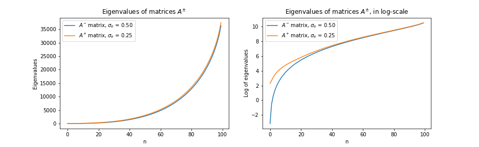
Figure 5: Eigenvalues of matrices ${\bf A}^{\pm}$ truncated at size $N=100$. On the left: Eigenvalues grow quadratically with $n$ for large values of $n$. On the right: eigenvalues are displayed in log-scale to show differences in spectra for ${\bf A}^{+}$ and ${\bf A}^{-}$.

The method of [16] thus elegantly uses the SUSY structure of the SE (A.10) to come up with a ‘natural’ countable basis for this problem. To proceed, we follow standard textbook steps, and look a solution in the form of an eigenstate decomposition with the basis (A.23) and time-dependent coefficients $w_{N}^{(F)}(t)$:

$$\Psi(x,\tau)=\sum_{n=0}^{\infty}w_{n}^{(F)}(\tau)\phi_{n}(x)$$ (A.26)

Here we denoted weights as $w_{n}^{(F)}(t)$ to differentiate them from weights $w_{N}^{(B)}(t)$ that will be introduced below for the BK-SE (19). We first use this relation to find the initial weights $w_{n}^{(F)}(0)$ at time 0. They can be found from the initial condition

$$\Psi(x,0)=\delta(x-x_{0})e^{\frac{V(x_{0}+\hat{z})}{\hbar}}$$ (A.27)

which follows from Eq.(21), and the completeness relation for basis functions

$$\sum_{n=0}^{\infty}\phi_{n}(x)\phi_{n}(x^{\prime})=\delta(x-x^{\prime})$$ (A.28)

This produces the initial weights

$$w_{n}^{(F)}(0)=\int_{-\infty}^{\infty}dx\Psi(x,0)\phi_{n}(x)=\int_{-\infty}^{\infty}dxe^{V(x)/\hbar}\delta(x-x_{0})\phi_{n}(x)=e^{V(x_{0})/\hbar}\phi_{n}(x_{0})$$ (A.29)

Note that $w_{n}^{(F)}(0)$ scale with $n$ for $n\rightarrow\infty$ as $n^{-1/4}\sin\left[2\sqrt{ny_{0}}-\pi\left(q-\frac{3}{4}\right)\right]$, as can be seen using the asymptotic expression for Laguerre polynomials for large values of $n$:

$$L_{n}^{(\alpha)}(x)=\frac{n^{\alpha/2-1/4}}{\sqrt{\pi}}x^{-\alpha/2-1/4}e^{x/2}\sin\left(2\sqrt{nx}-\frac{\pi}{2}\left(\alpha-1/2\right)\right)+O\left(n^{\alpha/2-3/4}\right)$$ (A.30)

A slow oscillating decay of initial weights with the basis index $n$ is illustrated in Fig. 6 on the left. Note that strong oscillations with $n$ are only observed for initial weights. Finite-$T$ weights for long enough times $T$ show a much smoother behavior with a fast decay of weights with $n$, as shown on the right of Fig. 6. Fig. 7 shows the behavior of finite-$T$ weights $w_{n}^{(F)}(T)$ as functions of $n$ for different planning horizons $T$, and shows that their decay with $n$ for sufficiently large values of $T$ such as $T=15$ or $T=20$ is exponential in $n$.

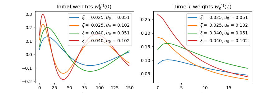
Figure 6: On the left: Initial weights $w_{n}^{(F)}(0)$ in Eq.(A.29) as a function of $n$ for different values of $u_{0}$. On the right: the finite-$T$ coefficients $w_{n}{(F)}(T)$ for $T=20$.

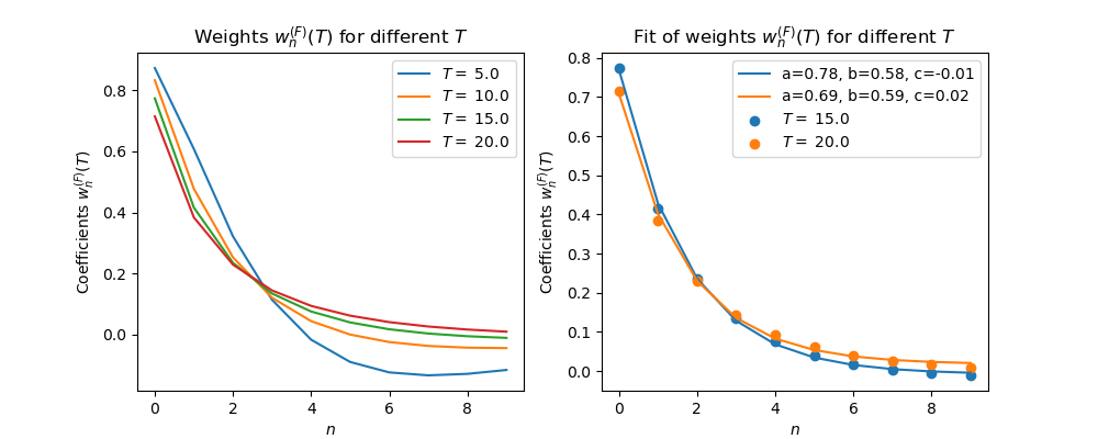
Figure 7: On the left: finite-$T$ weights $w_{n}(T)$ for the FP-SE (18) as functions of $n$ for different planning horizons $T$. Unlike initial weights $w_{n}(0)$ that decay as $n^{-1/4}$ with additional oscillations (see Fig. 6) on the left), weights for long times exhibit a fast and smooth decay with $n$. On the right: fit of weights $w_{n}(T)$ for $T=15$ and $T=20$ by the function $\hat{w}_{n}=ae^{-bn}+c$ with parameters $a,b,c$.

Still, while finite-$T$ coefficients $w_{n}^{F)}$ show a smooth regular behavior with a fast decay with $n$, the slow decay of initial weights $w_{n}^{F)}(0)$ might be concerning and pointing to a possible loss of accuracy for the FPE equation due to truncation of the original infinite-dimensional basis. It is therefore of interest to analytically explore implications of truncating the basis to a finite value of $N$ such as $N=100$ or $N=150$ for numerical implementation.

To begin, we start with an observation that a finite-$N$ approximation to the FPE density $f(x,0)$ is no longer exactly equal to $\delta(x-x_{0})$. Instead, it can be computed in closed form in terms of the Morse variable $y=y(x)=(2s+1)e^{-x}$ using Eq.(10.12.9) in [BE]:

$$\sum_{n=0}^{N-1}\frac{n!L_{n}^{(2q-1)}(x)L_{n}^{(2q-1)}(y)}{\Gamma(n+2q)}=\frac{N!}{\Gamma(N+2q-1)}\frac{1}{x-y}\left[L_{N-1}^{(2q-1)}(x)L_{N}^{(2q-1)}(y)-L_{N}^{(2q-1)}(x)L_{N-1}^{(2q-1)}(y)\right]$$ (A.31)

In the limit $N\rightarrow\infty$, this expression can be approximated as follows using the asymptotic form of $L_{n}^{(2q-1)}(x)$:

$$\sum_{n=0}^{N-1}\frac{n!L_{n}^{(2q-1)}(x)L_{n}^{(2q-1)}(y)}{\Gamma(n+2q)} = \frac{(xy)^{-q+1/4}e^{(x+y)/2}}{2\pi(x-y)}\left[\left(\sqrt{x}+\sqrt{y}\right)\sin\left(2\sqrt{N}(\sqrt{x}-\sqrt{y})\right)\right.$$ (A.32)

$$- \left.\left(\sqrt{x}-\sqrt{y}\right)\sin\left(2\sqrt{N}(\sqrt{x}+\sqrt{y})-2\pi(q-3/4)\right)\right]$$

The last relation can be used to explore the behavior of a finite-$N$ approximation to the FPE density $f(x,0)$ at time zero, which we will denote $f_{N}(x,0)$. We obtain

$$f_{N}(x,0) = \frac{1}{2\pi}y^{-1/2}\left(\frac{y}{y_{0}}\right)^{-\eta/\hbar-1/4}e^{-\frac{y-y_{0}}{2}}\left[\frac{\sin\left[2\sqrt{N}\left(\sqrt{y}-\sqrt{y_{0}}\right)\right]}{\sqrt{y}-\sqrt{y_{0}}}\right.$$

$$+ \left.\sin(2\pi q)\frac{\sin\left[2\sqrt{N}\left(\sqrt{y}+\sqrt{y_{0}}\right)\right]}{\sqrt{y}+\sqrt{y_{0}}}+\cos(2\pi q)\frac{\cos\left[2\sqrt{N}\left(\sqrt{y}+\sqrt{y_{0}}\right)\right]}{\sqrt{y}+\sqrt{y_{0}}}\right]$$

We now can use this expression to guide our choice for parameter $q>0$ which was considered a free parameter up to this point. In the strict limit $N\rightarrow\infty$, the first two terms in this expression converge, respectively, to $\delta(\sqrt{y}-\sqrt{y_{0}})$ and $\delta(\sqrt{y}+\sqrt{y_{0}})$, and furthermore the second delta-function $\delta(\sqrt{y}+\sqrt{y_{0}})$ vanishes for all values of $y_{0},y\neq 0$. On the other hand, the third term does not have a well-defined limit $N\rightarrow\infty$ for generic values of $q$. Therefore, we pick a value of $q$ that satisfies the relation $2\pi q=m\pi/2$ with $m=1,3,5,\ldots$, or equivalently

$$q=\frac{m}{4},\;\;\;\;m=1,3,5,\ldots$$ (A.34)

Furthermore, analysis of the probability current in this model performed in Appendix C shows that parameter $q$ should be larger than $\eta/\hbar$. As in our practical setting the ratio $\eta/\hbar$ varies approximately between -0.2 and 0.2, our final choice for $q$ corresponds to (A.34) with $m=3$:

$$q=\frac{5}{4}$$ (A.35)

Assuming this choice in (Appendix A: Schrödinger equation with the Morse potential) and transforming the delta-function $\delta(\sqrt{y}-\sqrt{y_{0}})$ back from the Morse variable $y=y(x)$ to the original $x$-space, we recover the correct initial condition in the limit $N\rightarrow\infty$:

$$\lim_{N\rightarrow\infty}f_{N}(x,0)=\delta(x-x_{0})$$ (A.36)

On the other hand, we see that for a finite $N$ approximation to the initial density $f(x,0)$ produces strong oscillations around the singular point $y=y_{0}$, see Fig. 8.

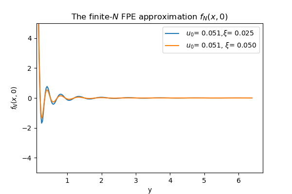
Figure 8: The finite-$N$ approximation for the FPE density $f_{N}(y,0)$ at $t=0$ with $N=150$, computed using Eq.(Appendix A: Schrödinger equation with the Morse potential) with $q=5/4$. Oscillations around the singular point $y=y_{0}$ are due to the truncation of the original infinite-dimensional basis.The correct initial state is proportional to $\delta(y-y_{0})$.

Now let us consider the BK-SE (19). For this equation, the only difference from the FP-SE (18) is in a different initial condition

$$\bar{\Psi}(x,0)=e^{-V(x)/\hbar}\theta(\hat{x}-x)$$ (A.37)

which follows from (21). This translates into different initial weights:

$$w_{N}^{(B)}(0)=\int_{-\infty}^{\infty}dx\phi_{n}(x)e^{-V(x)/\hbar}\theta(\hat{x}-x)$$ (A.38)

which gives

$$w_{N}^{(B)}(0)=\sqrt{\frac{n!}{\Gamma(n+2q)}}\int_{\hat{y}}^{\infty}dyz^{\kappa-1}e^{-y}L_{n}^{(2q-1)}(y)$$ (A.39)

where parameters $\hat{y}$ and $\kappa$ are defined as follows

$$\hat{y}=\frac{2u_{0}e^{\xi T}}{\hbar V_{\text{target}}},\;\;\;\kappa:=q-\eta/\hbar$$ (A.40)

Here $\hat{y}$ is the target value in terms of the Morse variable, and $\kappa=q-\eta/\hbar$ is an auxiliary parameter introduced to simplify formulae to follow. Note at this point that the integral in (A.39) can also be interpreted as the integral $\int_{\hat{y}}^{\infty}w_{n}^{(F)}(y)dy$ - which is of course as expected based on the Feynman-Kac representation (23) when combined with an eigenvalue decomposition method. This indicates that the method based on the BK-SE (A.3) should be preferable to the method based on the FP-SE (A.2) only if one or more of the following applies: (1) pre-asymptotic behavior for large but finite $N$ is better controllable within the BK-SE than the FP-SE, and (2) weights (A.39) can be efficiently computed, preferably in an analytical form.

Starting with the second item in this list, the weights $w_{N}^{(B)}(0)$ can be computed by writing the integral in (A.39) as the difference of two integrals on intervals $[0,\infty]$ and $[0,\hat{y}]$, and then using relations (7.414.11) and (7.415) from [7]:

$$\int_{\hat{y}}^{\infty}e^{-x}x^{\kappa-1}L_{n}^{(\alpha)}(x)dx = \frac{\Gamma(\kappa)\Gamma(\alpha+n+1-\kappa)}{n!\Gamma(\alpha+1-\kappa)}$$

$$- \frac{\Gamma(\kappa)\Gamma(\alpha+n+1)}{n!}\hat{y}^{\kappa}\operatorname{{\vphantom{\mathnormal{F}}}_{2}\kern-0.5pt\mathnormal{F}_{2}}(\alpha+n+1,\kappa;\alpha+1,\kappa+1;-\hat{y})$$

Here $\operatorname{{\vphantom{\mathnormal{F}}}_{2}\kern-0.5pt\mathnormal{F}_{2}}(a_{1},a_{2};b_{1},b_{2};z)$ is the generalized hypergeometric function $\operatorname{{\vphantom{\mathnormal{F}}}_{p}\kern-0.5pt\mathnormal{F}_{q}}(a_{1},\ldots,a_{p};b_{1},\ldots,b_{q};z)$ with $p=q=2$. The latter is defined, for generic values of $p,q$, by the following infinite series [1, BE]:

$$\operatorname{{\vphantom{\mathnormal{F}}}_{p}\kern-0.5pt\mathnormal{F}_{q}}(a_{1},\ldots,a_{p};b_{1},\ldots,b_{q};z)=\sum_{n=0}^{\infty}\frac{\left(a_{1}\right)_{n}\ldots\left(a_{p}\right)_{n}}{\left(b_{1}\right)_{n}\ldots\left(b_{q}\right)_{n}}\frac{z^{n}}{n!}$$ (A.42)

where $\left(x\right)_{n}:=\Gamma(x+1)/\Gamma(x+1-n)$ is the Pochhammer symbol. Recall that for symmetric cases $p=q$, including our case $p=q=2$, the generalized hypergeometric function $\operatorname{{\vphantom{\mathnormal{F}}}_{p}\kern-0.5pt\mathnormal{F}_{q}}({\bf a};{\bf b};z)$ is an entire function in the complex plane [1], so that the series (A.42) converges everywhere for this case, see Fig. 9. This enables a simple and numerically efficient implementation of $\operatorname{{\vphantom{\mathnormal{F}}}_{2}\kern-0.5pt\mathnormal{F}_{2}}(a_{1},a_{2};b_{1},b_{2};z)$, available e.g. in the Python package mpmath (https://mpmath.org) and Mathematica (https://www.wolfram.com). Weights $w_{n}^{(B)}(0)$ are then computed according to Eqs.(A.39) and (Appendix A: Schrödinger equation with the Morse potential).

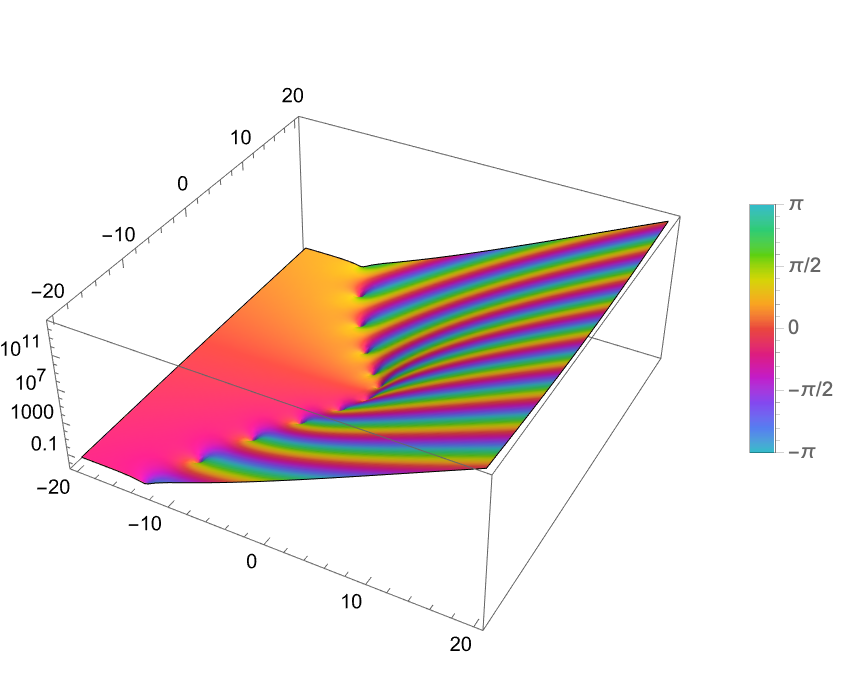
Figure 9: The generalized hypergeometric function ${}_{2}F_{2}(\alpha+n+1,\kappa;\alpha+1,\kappa+1;z)$ in the complex $z$-plane for $\alpha=3/2,\,\kappa=0.7$ and $n=10$. For $|z|\rightarrow\infty$, ${}_{2}F_{2}(\alpha+n+1,\kappa;\alpha+1,\kappa+1;z)\sim z^{n-1}e^{z}$.

Initial weights $w_{n}^{(B)}(0)$ computed according to (A.39) and (Appendix A: Schrödinger equation with the Morse potential) are shown together with their time-$T$ values in Fig. 10 for $T=20$. For comparison, in Fig. 11 we show coefficients $w_{n}^{(B)}(T)$ for different planning horizons $T$. Again, we observe an exponential decay of weights with $n$ for sufficiently large values of $T$, which is similar to the behavior observed for forward weights $w_{n}^{(F)}(T)$ in Fig. 7.

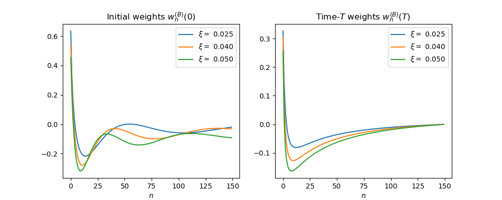
Figure 10: On the left: initial weights $w_{n}^{(B)}(0)$ for the BK-SE (19) as functions of $n$ for different values of $\xi$. On the right: time-$T$ weights $w_{n}^{(B)}(T)$ for $T=20$.

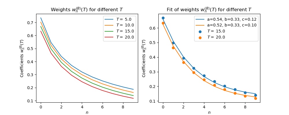
Figure 11: On the left: time-$T$ weights $w_{n}^{(B)}(T)$ for the BK-SE (19) as functions of $n$ for different values of $T$. On the right: fit of time-$T$ weights $w_{n}^{(B)}(T)$ for $T=15$ and $T=20$ by function $ae^{-bx}+c$.

To explore the large-$N$ behavior of $\bar{\Psi}_{N}(x,0)$, we again use (A.32) where we now set $q=5/4$ according to (A.35). Substituting this relation into the formula $\bar{\Psi}(x,0)=\sum_{n}w_{n}^{(B)}(0)\phi_{n}(x)$ with weights $w_{n}^{(B)}(0)$ defined by Eq.(A.39), we obtain the following formula for a large-$N$ approximation $\bar{\Psi}_{N}(x,0)$ to the initial state $\bar{\Psi}(x,0)$:

$$\bar{\Psi}_{N}(x,0)=\frac{y^{1/4}}{2\pi}\int_{\hat{y}}^{\infty}dzz^{\kappa-2}e^{-z/2}\left(\frac{\sin\left[2\sqrt{N}(\sqrt{z}-\sqrt{y})\right]}{\sqrt{z}-\sqrt{y}}+\frac{\sin\left[2\sqrt{N}(\sqrt{z}+\sqrt{y})\right]}{\sqrt{z}+\sqrt{y}}\right)$$ (A.43)

In the limit $N\rightarrow\infty$, we use the relation

$$\lim_{N\rightarrow\infty}\frac{\sin\left[2\sqrt{N}(\sqrt{z}-\sqrt{y})\right]}{\sqrt{z}-\sqrt{y}}=\pi\delta(\sqrt{z}-\sqrt{y})=2\pi\sqrt{y}\delta(z-y)$$ (A.44)

to obtain

$$\lim_{N\rightarrow\infty}\bar{\Psi}_{N}(x,0)=y^{\kappa-5/4}e^{-y/2}\theta(y>\hat{y})$$ (A.45)

The contribution of the second term in (A.43) vanishes in the limit $N\rightarrow\infty$ as it is proportional to $\delta(\sqrt{y}+\sqrt{\hat{y}})$. Therefore we obtain

$$\lim_{N\rightarrow\infty}p_{N}(x+\hat{z},0)=\lim_{N\rightarrow\infty}e^{V(x+\hat{z})/\hbar}\bar{\Psi}_{N}(x,0)=\theta(y>\hat{y})$$ (A.46)

consistently with the initial condition (21). Therefore, we verified that the correct initial condition for $p_{N}(x+\hat{z},0)$ is recovered in the strict limit $N\rightarrow\infty$. On the other hand, as in practice we have to work with a finite $N$, it is important to estimate pre-asymptotic corrections to $\bar{\Psi}_{N}(x,0)$ and $p_{N}(x+\hat{z},0)$ for large but finite values of $N$. Calculation of these corrections is presented in Appendix B, and produces the following result (here $\omega:=2\sqrt{N}$):

$$\bar{\Psi}_{\omega}(x,0)=y^{\kappa-5/4}e^{-y/2}\theta(y>\hat{y})-\frac{2y^{-1/4}\hat{y}^{\kappa-\frac{3}{2}}\sin\left(\omega\sqrt{\hat{y}}\right)}{\pi\omega}\left[\cos\left(\omega\sqrt{y}\right)+\sin\left(\omega\sqrt{y}\right)\right]+O\left(\frac{1}{\omega^{2}}\right)$$ (A.47)

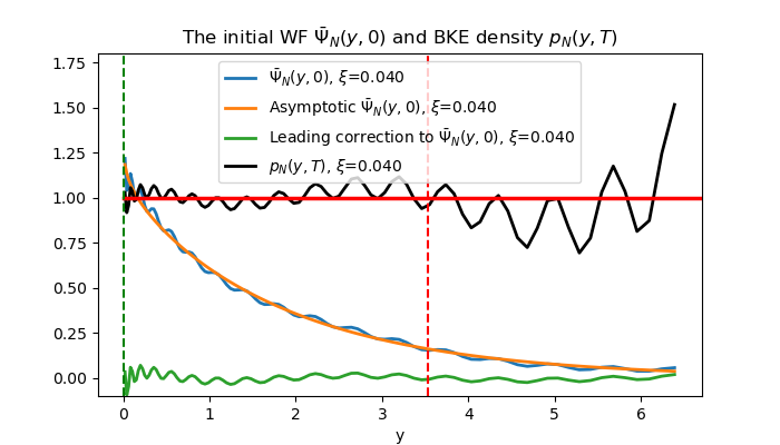
Figure 12: Finite-$N$ approximation to the time-0 WF $\hat{\Psi}_{N}(y,0)$ and the terminal BKE tail probability $p_{N}(y,T)$ computed according to (A.47). With $N=150$, the finite-$N$ BKE density $p_{N}(y,T)$ is an approximation to the true limit $p_{\infty}(y,T)=\theta(y-\hat{y})$ which is only recovered in the strict limit $N\rightarrow\infty$. Increasing oscillations for large values of $y$ indicate that corrections not included in (A.47) become important in this region.

The initial BK-SE WF $\bar{\Psi}(y,0)$ and the terminal BKE density $p_{N}(y,T)$ computed using Eq.(A.47) are shown in Fig. 12. A few comments can be made at this point. First, we observe that corrections to the asymptotic result given by the first term depend not just on the value of $N$ but rather on the combinations $2\sqrt{Ny}$ and $2\sqrt{N\hat{y}}$. Second, corrections grow in the relative sense when $y\rightarrow\infty$, showing that Eq.(B.14) is an asymptotic expansion valid only for sufficiently small values of $y$ such that corrections are still smaller than the leading asymptotic term $e^{-y/2}\theta(y>\hat{y})$. Note that the leading correction in (B.14) formally becomes a dominant term in the limit $y\rightarrow\infty$, because it does not have an exponential term. As the correct asymptotic behavior of the model at $y\rightarrow\infty$ is actually given by the leading term $e^{-y/2}\theta(y>\hat{y})$, it simply means that for larger values of $y$ more and more terms in the eigenvalue decomposition become important. In the limit $y\rightarrow\infty$, the whole infinite basis is required to produces the correct behavior.

Third, Fig. 12 compares the finite-$N$ approximation to the BKE terminal density $p_{N}(y,T)$ to its true asymptotic form $\theta(y-\hat{y})$. This analysis suggests that the BK-SE (A.3) may be more forgiving to a truncation of the infinite-dimensional basis than the related FP-SE (A.10). This can be based on the observation that at least with $N=150$, our terminal BKE density $p_{N}(y,T)$ looks more similar to its correct $N\rightarrow\infty$ limit $\theta(y>\hat{y})$ than the time-0 FPE density $f_{N}(y,0)$ looks similar to the delta-function $\delta(y-y_{0})$ in Fig. 8. Note that while the finite-$N$ density $p_{N}(y,T)$ shows that corrections to the asymptotic expression become large for large values of $y$, our approach is not expected to loose much accuracy due to the truncation as long as values of $y$ of interest are still below this threshold.

Provided we use different initial weights given by (A.29) for the FP-SE (18) or (A.38) for the BK-SE (19), all subsequent steps are the same for both equations. Substituting (A.26) into the SE (A.10), multiplying both sides by $\phi_{m}(x)$ and integrating over $x$, we end up with a system of ordinary differential equations (ODEs) for coefficients $w_{n}(\tau)$ which can be written in a vector form as follows:

$$-\frac{d{\bf w}(\tau)}{d\tau}={\bf A}^{\pm}{\bf w}(\tau)$$ (A.48)

where we should ${\bf A}_{+}$ or ${\bf A}_{-}$ when $g>0$ or $g<0$, respectively. The solution to this system of ODEs read

$${\bf w}(\tau)=e^{-\tau{\bf A}^{\pm}}{\bf w}(0)={\bf U}_{\pm}e^{-\tau\text{\boldmath$\mathcal{D}$}_{\pm}}{\bf U}_{\pm}^{T}{\bf w}(0)$$ (A.49)

where ${\bf w}(0)$ is a vector of initial weights (A.29) or (A.38), and we used (A.25) in the second equation. The behavior of weights $w_{n}(T)$ for different values of $T=[5,10,15,20]$ is shown in Figs. 7 and 11 for the FPE and BKE equations, respectively. As found in both cases, the dependence of weights $w_{n}^{F)}(T)$ or $w_{n}^{B)}(T)$ on $n$ for long enough time horizons $T$ is well approximated by the formula $w_{n}\simeq ae^{-bn}+c$ where parameters $a,b,c$ depend on $T$.

The time-dependent solution of the FP-SE (A.2) is now computed as follows:

$$\Psi(x,t)={\bf w}_{F}^{T}(0)e^{-\frac{h}{2}t{\bf A}^{\pm}}\text{\boldmath$\phi$}(x)$$ (A.50)

where we now denoted the FP-SE weights (A.29) as ${\bf w}_{F}(0)$. Now we can use Eqs.(Appendix A: Schrödinger equation with the Morse potential) and (C.3), we obtain the FPE density in the $y$-space as follows:

$$f(y,t)=y^{-1}e^{-V(y)/\hbar}\Psi(y,t)=y^{\eta/\hbar-1}e^{-y/2}\Psi(y,t)$$ (A.51)

Comparing (A.51) with (A.50), we see that the FPE density $f(z,t)$ has the same functional form as the quantum-mechanical WF (A.50), albeit with different coefficients, see Fig. 13.

In its turn, the solution for BK-SE (A.3) is computed as follows:

$$\bar{\Psi}(x,t)={\bf w}_{B}^{T}(0)e^{-\frac{h}{2}\left(T-t\right){\bf A}^{\pm}}\text{\boldmath$\phi$}(x)$$ (A.52)

where weights ${\bf w}_{B}^{T}(0)$ are computed according to (A.38). Using Eqs.(Appendix A: Schrödinger equation with the Morse potential), we obtain the solution for the BKE:

$$p(y,t)=e^{V(y)/\hbar}\Psi(y,t)=y^{-\eta/\hbar}e^{y/2}\bar{\Psi}(y,t)$$ (A.53)

Eqs.(A.50), (A.52), (A.51), (A.53) provide our final semi-analytical expressions for the quantum-mechanical WFs $\Psi(x,t),\,\bar{\Psi}(x,t)$ and the FPE and BKE densities $f(z,t),\,p(z,t)$, respectively. The behavior of the resulting densities is illustrated in Fig. 13.

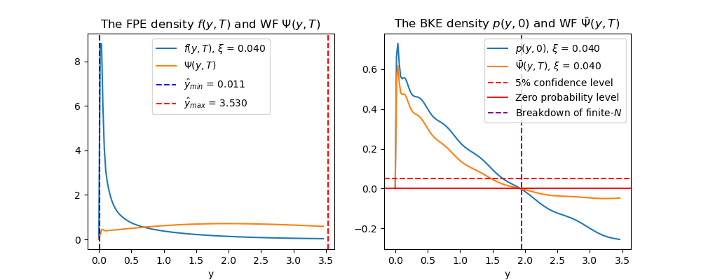
Figure 13: On the left: The FPE density $f(y,T)$ and quantum mechanical wave function $\Psi(y,T)$ for $T=20$. The FPE density $f(y,T)$ has a sharp peak at a small value $y=y_{\star}$, and monotonically decays for $y>y_{\star}$. On the right: the BKE tail probability $p(y,0)$ and quantum mechanical wave function $\bar{\Psi}(x,T)$ for $T=20$. The BKE density has a maximum at a small value of $y$, and monotonically decays to the right of this point. The vertical line denoted ’Breakdown of finite-$N$’ shows the value of $y$ where $\bar{\Psi}(y,t)$ becomes slightly negative due to the basis truncation.

Appendix B: Asymptotic expansion of $\bar{\Psi}_{N}(x,0)$

In this appendix, we compute a leading pre-asymptotic correction to $\bar{\Psi}_{N}(x,0)$ defined in Eq.(A.43). It is convenient at this stage to introduce the parameter $\omega:=2\sqrt{N}$, so that Eq.(A.43) takes the following form:

$$\bar{\Psi}_{\omega}(x,0)=\frac{y^{1/4}}{2\pi}\int_{\hat{y}}^{\infty}dzz^{\kappa-2}e^{-z/2}\left(\frac{\sin\left[\omega(\sqrt{z}-\sqrt{y})\right]}{\sqrt{z}-\sqrt{y}}+\frac{\sin\left[\omega(\sqrt{z}+\sqrt{y})\right]}{\sqrt{z}+\sqrt{y}}\right)$$ (B.1)

To compute the pre-asymptotic correction, we use the identity

$$\bar{\Psi}_{\omega}(x,0)=\bar{\Psi}_{\infty}(x,0)-\int_{\omega}^{\infty}\frac{\partial\bar{\Psi}_{\omega^{\prime}}(x,0)}{\partial\omega^{\prime}}d\omega^{\prime}:=\bar{\Psi}_{\infty}(x,0)+\Delta_{\omega}\bar{\Psi}(x.0)$$ (B.2)

where

$$\bar{\Psi}_{\infty}(x,0):=\lim_{\omega\rightarrow\infty}\bar{\Psi}_{\omega}(x,0)=y^{\kappa-5/4}e^{-y/2}\theta(y>\hat{y})$$ (B.3)

Therefore, we have to compute the asymptotics of the second term $\Delta_{\omega}\bar{\Psi}(x.0)$ in (B.2). Note that we have $\lim_{\omega\rightarrow\infty}\Delta_{\omega}\bar{\Psi}(x,0)=0$ by construction. To tackle the semi-infinite integration range $[\omega,\infty]$ in (B.2), we use the Bromwich integral representation of the Heaviside step-function:

$$\theta(x)=\frac{1}{2\pi i}\int_{\varepsilon-i\infty}^{\varepsilon+i\infty}dz\frac{e^{xz}}{z}$$ (B.4)

along with Eqs.(3.462) and (9.246.3) from [7]. This produces the following expression for the derivative $\partial{\bar{\Psi}}_{N}/\partial\omega$ in the limit $\omega\gg 1$:

$$\frac{\partial\bar{\Psi}_{N}(x,0)}{\partial\omega}=-\frac{2\Gamma(2\kappa-2)}{\pi}y^{\frac{1}{4}}\cos\left(\omega\sqrt{y}\right)\text{Re}\left[\frac{e^{i\pi\kappa}}{2\pi i}\int_{\varepsilon-i\infty}^{\varepsilon+i\infty}dz\frac{e^{-z\sqrt{\hat{y}}}}{z}\left[\left(\omega-iz\right)^{2-2\kappa}+\rho\left(\omega-iz\right)^{-2\kappa}+\ldots\right]\right]$$ (B.5)

where $\rho=(1-\kappa)(1-2\kappa)$, and ellipses stand for higher powers of $1/(\omega-iz)$. Plugging this back into (B.2) and interchanging the order of integration with respect to $\omega$ and $z$, we obtain:

$$\Delta_{\omega}\bar{\Psi}(x.0)=\frac{4\Gamma(2\kappa-2)}{\pi}y^{1/4}\text{Re}\left[\frac{e^{i\pi\kappa}}{2\pi i}\int_{\varepsilon-i\infty}^{\varepsilon+i\infty}dz\frac{e^{-z\sqrt{\hat{y}}}}{z}\left[J\left(z,\omega,\nu_{1}\right)+\rho J\left(z,\omega,\nu_{2}\right)+\ldots\right]\right]$$ (B.6)

where $\nu_{1}=2-2\kappa$, $\nu_{2}=-2\kappa$, $\kappa=q-\eta/\hbar$ and $J(z,\omega,\nu)$ stands for the inner integral with respect to $\omega^{\prime}$:

$$J(z,\omega):=\int_{\omega}^{\infty}d\omega^{\prime}\cos\left(\omega^{\prime}\sqrt{y}\right)(\omega^{\prime}-iz)^{\nu}$$ (B.7)

The integral $J(z,\omega,\nu)$ can be computed using Eqs.(3.761.2) and (3.761.7) from [7]:

$$J(z,\omega,\nu)=\frac{iy^{-\frac{\nu}{2}-\frac{1}{2}}}{2}\left[e^{-z\sqrt{y}-i\frac{\pi}{2}(\nu+1)}\Gamma\left(\nu+1,i\sqrt{y}(\omega-iz)\right)-e^{z\sqrt{y}+i\frac{\pi}{2}(\nu+1)}\Gamma\left(\nu+1,-i\sqrt{y}(\omega-iz)\right)\right]$$ (B.8)

While this expression gives an exact value of the integral for arbitrary $\omega$, as we use asymptotic relations in other parts of our derivation, we can only retain the leading terms that survive in the limit $\omega\rightarrow\infty$. This is achieved using the asymptotic expansion of the incomplete gamma function $\Gamma(\nu,x)$ given by Eq.(8.357) in [7]:

$$\Gamma(\nu,x)=x^{\nu-1}e^{-x}\left[1-(1-\nu)x^{-1}+\ldots\right],\;\;\;|x|\rightarrow\infty$$ (B.9)

This gives the following asymptotic form for the integral $J(z,\omega,\nu)$ valid in the limit $\omega\gg 1$:

$$J(z,\omega,\nu)=-y^{-\frac{1}{2}}\left[\left(\omega-iz\right)^{\nu}\sin\left(\omega\sqrt{y}\right)+\nu y^{-\frac{1}{2}}\left(\omega-iz\right)^{\nu-1}\cos\left(\omega\sqrt{y}\right)+O\left(\left(\omega-iz\right)^{\nu-2}\right)\right]$$ (B.10)

Substituting this back into (B.6), we obtain

$$\Delta_{\omega}\bar{\Psi}(x.0)=-\frac{2\Gamma(2k-2)}{\pi}y^{-1/4}\left[\sin\left(\omega\sqrt{y}\right)I(\hat{y},\kappa)+2(1-\kappa)\cos\left(\omega\sqrt{y}\right)I(\hat{y},\kappa+\frac{1}{2})+\ldots\right]$$ (B.11)

where

$$I(\hat{y},\kappa):=\text{Re}\left[\frac{e^{i\pi\kappa}}{2\pi i}\int_{\varepsilon-i\infty}^{\varepsilon+i\infty}dz\frac{e^{-z\sqrt{\hat{y}}}}{z}\left(\omega-iz\right)^{2-2\kappa}\right]$$ (B.12)

This last integral can be transformed into a a closed contour integral by adding a semi-circle in the positive semi-plane at $|z|\rightarrow\infty$. The remaining contour integral can now be deformed to run from $\infty$ to $0$ above the branch cut on $[0,\infty]$, and then back from $0$ to $\infty$ under the branch cut. As the total value of the contour integral is zero, we obtain that the Bromwich integral arising in (B.11) is given by the difference of two integrals $I_{+}$ and $I_{-}$ where the first integral runs from $0$ to $\infty$ with $z=x$ with a real value of $x$, while the second integral $I_{-}$ runs from $\infty$ to $0$ with $z=e^{2i\pi}x$. Due to the branch cut singularity, the two integrals do not cancel out. Instead, we find that $I_{-}=-e^{4i\pi\kappa}I_{+}$. This produces the following result for the integral (B.12):

$$I(\hat{y},\kappa)=\frac{\sin(2\pi\kappa)}{\pi}\left[\frac{\Gamma(3-2\kappa)}{\omega}\hat{y}^{\kappa-\frac{3}{2}}\sin\left(\omega\sqrt{\hat{y}}\right)-\frac{\Gamma(4-2\kappa)}{\omega^{2}}\hat{y}^{\kappa-2}\cos\left(\omega\sqrt{\hat{y}}\right)\right]$$ (B.13)

Plugging this into (B.11) and using (B.2), we finally obtain

$$\bar{\Psi}_{\omega}(x,0)=y^{\kappa-5/4}e^{-y/2}\theta(y>\hat{y})-\frac{2y^{-1/4}\hat{y}^{\kappa-\frac{3}{2}}\sin\left(\omega\sqrt{\hat{y}}\right)}{\pi\omega}\left[\cos\left(\omega\sqrt{y}\right)+\sin\left(\omega\sqrt{y}\right)\right]+O\left(\omega^{-2}\right)$$ (B.14)

We see that pre-asymptotic corrections die off very slowly $\sim N^{-1/2}$ times oscillating $\sin$ functions depending on $2\sqrt{Ny}$ and $2\sqrt{N\hat{y}}$. Eq.(B.14) is an asymptotic expansion valid only for sufficiently small values of $y$ such that the correction is still smaller than the leading asymptotic term $e^{-y/2}\theta(y>\hat{y})$. Note that the correction in (B.14) formally becomes a dominant term in the limit $y\rightarrow\infty$, because it does not have a decaying exponential factor which appears in the first term. As the correct asymptotic behavior of the model at $y\rightarrow\infty$ is actually given by the leading term $e^{-y/2}\theta(y>\hat{y})$, it simply means that for larger values of $y$ more and more terms in the eigenvalue decomposition become important. In the limit $y\rightarrow\infty$, the whole infinite basis is required to produce the correct behavior. Fortunately, the strict limit $y\rightarrow\infty$ is mostly of academic interest, and in practice the actual values of $y$ of interest for the BKE may lie well below the onset of such region.

Appendix C: Probability current and constraints on parameter $q$

In this appendix, we analyze probability conservation and implications of the basis truncation for the FPE and FP-SE, and show how this analysis is used in order to pick a proper value of our hyperparameter $q$.

The analysis below is based on another useful form for the FPE (14) that expresses it in the form of a continuity equation

$$\frac{\partial f(x,t)}{\partial t}=\frac{\partial}{\partial x}J(x,t),\;\;\;J(x,t):=\frac{\partial V}{\partial x}f(x,t)+\frac{\sigma^{2}}{2}\frac{\partial f(x,t)}{\partial x}$$ (C.1)

where $J(x,t)$ is the probability current. Written in this form, the FPE shows that to conserve the total probability $\int f(x,t)dx$, the probability current $J(x,t)$ should vanish at $x\rightarrow\pm\infty$.

It is instructive to start with verifying the conservation of probability for the expansion (A.26). According to (Appendix A: Schrödinger equation with the Morse potential), the normalization constraint $\int f(x,t)dx=1$ for the FPE implies the following relation for the weights $w_{n}^{(F)}$:

$$\int_{-\infty}^{\infty}f(x,t)dx=\int_{-\infty}^{\infty}e^{-V(x)/\hbar}\Psi(x,t)dx=\sqrt{\Gamma(2q)}\sum_{n=0}^{\infty}w_{N}^{(F)}(\tau)\int_{0}^{\infty}y^{\eta/\hbar-q-1}\phi_{0}(y)\phi_{n}(y)dy$$ (C.2)

Here in the second equation we used the relation

$$e^{-V(x)/\hbar}=y^{\eta/\hbar}e^{-y/2}=\sqrt{\Gamma(2q)}y^{\eta/\hbar-q}\phi_{0}(y)$$ (C.3)

Comparing Eq.(C.2) with the orthonormality condition $\int dx\phi_{n}(x)\phi_{m}(x)=\int\frac{dy}{y}\phi_{n}(y)\phi_{m}(y)=\delta_{mn}$, it could be tempting to set $q=\eta/\hbar$ here so that we would have

$$e^{-V(x)/\hbar}\Psi(x,\tau)\sim\phi_{0}(y)\sum_{n=0}^{\infty}w_{N}^{(F)}(\tau)\phi_{n}(y)$$ (C.4)

which would automatically preserve the total normalization due to orthogonality of the basis, as the right hand of this equation would then integrate to one provided the weights sum up to one. However, as we will see shortly, we are not free to pick the value $q=\eta/\hbar$, as such choice produces a diverging probability current at infinity.

Back to Eq.(C.2) and computing the integral in it, we obtain

$$\int_{-\infty}^{\infty}f(x,t)dx=\frac{\Gamma(q+\eta/\hbar)}{\Gamma(q-\eta/\hbar)}\sum_{n=0}^{\infty}\frac{\Gamma(n+q-\eta/\hbar)}{\sqrt{n!\Gamma(n+2q)}}w_{n}(\tau)$$ (C.5)

Note that this expression is linear, rather than quadratic in weights $w_{n}(\tau)$, as would be the case in the conventional quantum mechanics [12]. A different normalization in our case is due to Eq.(Appendix A: Schrödinger equation with the Morse potential) which fixes the normalization rule for $\Psi(x,\tau)$, and replaces here the standard quantum mechanical normalization rule $\int\left|\Psi(x,\tau)\right|^{2}dx=1$ which translates into the constraint $\sum_{n}w_{n}^{2}(\tau)=1$ in terms of the eigenvalue expansion (A.26).

The initial value of the total probability (C.5) can be computed explicitly using Eq.(A.29):

$$\int_{-\infty}^{\infty}f(x,0)dx = y_{0}^{q-\eta/\hbar}\frac{\Gamma(q+\eta/\hbar)}{\Gamma(q-\eta/\hbar)}\sum_{n=0}^{\infty}\frac{\Gamma(n+q-\eta/\hbar)}{\Gamma(2q+n)}L_{n}^{(2q-1)}(y_{0})$$ (C.6)

$$= y^{q-\eta/\hbar}(x_{0})y^{-q+\eta/\hbar}(x_{0})=1$$

Here in the second line we used the expansion of a power function $f(x)=x^{-p}$ in Laguerre polynomials

$$x^{-p}=\frac{\Gamma(\alpha+1-p)}{\Gamma(p)}\sum_{n=0}^{\infty}\frac{\Gamma(n+p)}{\Gamma(n+\alpha+1)}L_{n}^{(\alpha)}(x),\;\;\;(p>0)$$ (C.7)

If we take $p=q-\eta/\hbar$ in (C.7), we verify the last equation in (C.6). Importantly, as Eq.(C.7) requires that $p>0$, we obtain that

$$q>\frac{\eta}{\hbar}$$ (C.8)

This calculation shows that the FPE density is correctly normalized at time $t=0$ due to Eq.(C.7), provided (C.8) is satisfied. While necessary, this condition is not sufficient on its own to provide a well-behaved model. In particular, we note that Eq.(C.8) only gives a formal answer for an infinite sum. When the infinite sum in (C.7) is truncated to a finite sum as is done in practice, convergence properties of the infinite series become important.

For the series, (C.7), the convergence criterion amounts to the requirement that the integral $\int_{0}^{\infty}x^{\alpha}e^{-x}x^{-2p}dx$ should stay finite. When we set here $p=q-\eta/\hbar$ and $\alpha=2q-1$, this translates into the constraint $\eta/\hbar>0$. However, this constraints does not always hold in our practical setting, where typical values of $\eta/\hbar$ vary approximately in the range $[-0.2,0.2]$. When $\eta/\hbar<0$, the Taylor expansion (C.7) becomes an asymptotic series rather than a converging series. Unlike converging series, coefficients in asymptotic series may produce diverging patterns.

The asymptotic character of the Taylor expansion (C.7) with $p=q-\eta/\hbar$ when $\eta/\hbar<0$ can be seen as follows. The combinatorial factor $\Gamma(n+q-\eta/\hbar)/\Gamma(n+2q)$ scales for $n\rightarrow\infty$ as $n^{-q-\eta/\hbar}$, and the Laguerre polynomials $L_{N}^{(2q-1)}(x)$ scale as $n^{q-3/4}\sin\left(2\sqrt{nx}+\phi\right)$ where $\phi$ is a phase parameter. Therefore, the coefficients in (C.6) scale as $n^{-\eta/\hbar-3/4}\sin\left(2\sqrt{ny_{0}}+\phi\right)$. Approximating the residual sum by an integral, we have an analytical expression for the residual of the infinite sum in (C.6):

$$P_{>N} := y_{0}^{q-\eta/\hbar}\frac{\Gamma(q+\eta/\hbar)}{\Gamma(q-\eta/\hbar)}\sum_{n=N}^{\infty}\frac{\Gamma(n+q-\eta/\hbar)}{\Gamma(2q+n)}L_{n}^{(2q-1)}(y_{0})$$ (C.9)

$$= y_{0}^{q-\eta/\hbar}\frac{\Gamma(q+\eta/\hbar)}{\Gamma(q-\eta/\hbar)}\int_{N}^{\infty}x^{-\eta/\hbar-3/4}\sin\left(2\sqrt{y_{0}x}+\phi\right)dx+\ldots$$

where ellipses stand for terms suppressed by powers of $1/N$. This integral can be computed exactly in terms of incomplete gamma functions using Eqs.(3.761.2) and (3.761.7) in [7], and it converges under the constraint

$$\eta/\hbar>-1/4$$ (C.10)

In the limit $\omega\rightarrow\infty$, the resulting expression considerably simplifies, and we obtain:

$$P_{>N}=\frac{\Gamma(q+\eta/\hbar)}{\Gamma(q-\eta/\hbar)}y_{0}^{q-1/4}\left(y_{0}N\right)^{-\eta/\hbar-1/4}\cos\left(\sqrt{y_{0}N}-\pi\left(q-3/4\right)\right)+O\left(\frac{1}{\omega^{2}}\right)\;\;\;\frac{\eta}{\hbar}>-\frac{1}{4}$$ (C.11)

Fortunately the constraint $\eta/\hbar>-1/4$ is typically satisfied for cases of practical interest for our problem, where it ranges approximately in the interval $[-0.2,0.2]$. Also note that Eq.(C.11) shows that for short times, the eigenvalue expansion is an asymptotic series rather than a converging series. The value of the residual sum $P_{>N}$ for a fixed $N$ depends on the product $Ny_{0}$ where $y_{0}$ is the initial value of the Morse variable, and Eq.(C.11) implies that the value of $Ny_{0}$ is such that the whole expression is between 0 and 1 - which would not be guaranteed for an arbitrary large value of $N$ given the value of $y$ due to the presence of the $\cos$ function in (C.11).

When $\eta/\hbar>-1/4$, a finite-$N$ approximation of the basis gives rise to strong oscillations up to moderately high values of $N\sim 100-200$, see Fig 14. These oscillations are due to in the oscillations of coefficients $w_{n}(0)$ shown above in Fig. 6. Furthermore, a finite-$N$ approximation also introduces an artificial dependence of the norm of the FPE density on the initial value $y_{0}$ - which in fact exactly cancels out in (C.6).

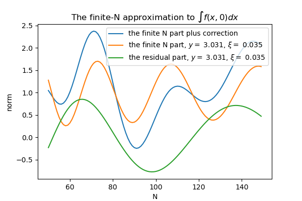
Figure 14: Finite-$N$ approximation to the infinite series in Eq.(C.6) as a function of $N$. The blue line shows the result of a finite-$N$ truncation with a correction computed using Eq.(C.11). In this figure, we chose to show the behavior for a large value of $y_{0}$, where corrections become of the same order as the leading term. For smaller values of $y_{0}$, the leading correction is considerably smaller than the leading term, which justifies the use of asymptotic estimations in this case.

We see that while the correct normalization of the FPE density at $t=0$ is guaranteed in our theory, it critically depends on keeping the full infinite-dimensional basis. Related to this observation, and also implied by the principle of continuity, eigenvalue decomposition methods for the SE or FPE are known to perform poorly for short times due to a slow convergence, and thus are simply not a method of choice when the main focus of research is on a short-term behavior. Fortunately, in our problem we are instead interested in a long-term behavior, where eigenvalue decomposition methods for PDEs usually work considerably better.

On the other hand, the problem still persists in practice. A finite-$N$ truncation of the infinite basis needed for a numerical implementation creates initially unnormalized densities. As we have seen above, for long times of interest for this study $T\simeq 15-20$, weights decays with $n$ very fast for both the forward and backward problems, as shown in Figs. 7 and 11. Nevertheless, the initial error in normalization due to the basis truncation propagates to time horizons of interest, at least with $N=150$ (using $N=200$ produced similar results), see Figs. 15 and 16. Norms of FPE densities for different time horizons show deviations from the unit normalization of the order of one percent for the range of parameters of interest.

A properly normalized initial density can of course be obtained by dividing the unnormalized density by its total integral computed numerically. However, for our practical objective of comparing distributions corresponding to different values of control parameters $u_{0}$ and $\xi$, such approach can introduce some spurious behavior. In particular, our objective should be a monotonically increasing along both dimensions $u_{0}$ and $\xi$. On the other hand, given that initial weights $w_{n}(0)$ show a slow oscillatory decay, normalization of the initial FPE density $f(x,0)$ by such procedure could introduce some non-monotonicity in the resulting behavior of our model.

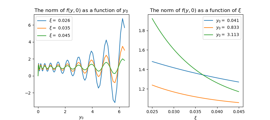
Figure 15: The norm of the time-$0$ FPE density (A.51) for $T=20$, computed using $N=150$ basis functions. On the left: the norm as a function of initial contribution $u_{0}$ (shown here in units of the Morse variable y). One the right: the normalization factor as a function of contribution growth rate $\xi$. Deviations of the norm from unity are due to the truncation of the infinite-dimensional basis to a finite basis of size $N$.

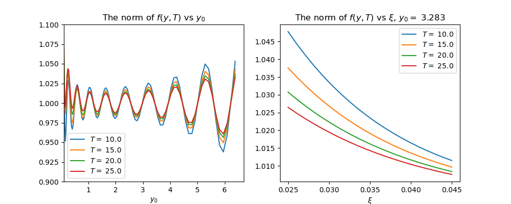
Figure 16: The norm of the finite-$T$ FPE density (A.51) for different values of $T$, computed using $N=150$ basis functions. On the left: the norm as a function of initial contribution $u_{0}$ (shown here in units of the Morse variable $y$), with a fixed value of $\xi$. One the right: the norm as a function of contribution growth rate $\xi$, with a fixed value of $u_{0}$. Deviations of the norm from unity are due to the truncation of the infinite-dimensional basis to a finite basis of size $N$.

To summarize to this point, pre-asymptotic corrections in expansions of FK-SE (18) and BK-SE (19) given, respectively, by Eqs.(C.11) and (B.14) show a similar behavior of both solutions as functions of $1/\sqrt{N}$, with oscillations and a slow power-like decay in the basis truncation number $N$. When model parameters are taken to be in a range corresponding to real-world scenarios, we find that both the forward and backward models combined with the eigenvalue decomposition amount to asymptotic series in this regime. The similarity of the behavior of both WFs is of course not accidental as they are related by the Feynman-Kac relation (22).

In practice, when working with asymptotic series truncated at the $N$-th term, the important point to remember is that taking the largest possible value of $N$ may not be the best idea. Instead, by analyzing relations such as (C.11) and (B.14), and noticing that results depend on combinations of $N$ with other inputs (the products $Ny$ and $Ny_{0}$, in our case), a good value of $N$ can be picked by the requirement that the pre-asymptotic correction should vanish, or that the partial sum in the expansion be stationary for an optimal value of $N$. Such tricks usually considerably improve models involving asymptotic expansions, see e.g. [15]. If our problem had fixed values of $y$ or $y_{0}$, we could use (C.11) and/or (B.14) to pick a value of $N$ such that the leading correction to the asymptotic formula would vanish. Unfortunately, doing this could be problematic in the setting of the present work where the values of $y$ and $y_{0}$ in Eqs.(C.11) and (B.14) are not fixed but instead serve as decision variables. Making $N$ dependent on $y$ or $y_{0}$ could introduce spurious non-monotonicity in the output BKE tail probability viewed as a function of control variables, and therefore we have not attempted such tricks for improving the behavior of asymptotic series.

To verify that there is no non-vanishing probability flux at the spatial infinity, we compute the probability current $J(z,t)$ as defined in Eq.(C.1). Using Eq.(Appendix A: Schrödinger equation with the Morse potential), we obtain:

$$J(x+\hat{x},t)=\frac{\hbar}{2}e^{-V(x+\hat{z})/\hbar}\left(\frac{1}{\hbar}\frac{\partial V}{\partial x}\Psi(x,t)+\frac{\partial\Psi}{\partial x}\right)=\frac{\hbar}{2}e^{-V(x+\hat{z})/\hbar}\mathcal{Q}\left(\eta/\hbar\right)\Psi(x,t)$$ (C.12)

To evaluate (C.12), we use Eqs.(A.26), (Appendix A: Schrödinger equation with the Morse potential) and (C.3). This produces the following expression:

$$J(y,t)=\frac{\hbar}{2}y^{\eta/\hbar}e^{-y/2}\sum_{n=0}^{\infty}w_{n}(t)\left[\mathcal{Q}(q+n)-\left(\frac{\eta}{\hbar}+q+n\right)\right]\phi_{n}(y)$$ (C.13)

As the infinite sum in in this expression behaves in the limit $y(x)\rightarrow 0$ as $y^{q}$, we obtain the $\left.J(y,t)\right|_{y\rightarrow 0}\propto y^{\eta/\hbar+q}$. This shows that the requirement of vanishing probability current at $y=0$ produces the following constraint for our hyperparameter $q$:

$$q>-\frac{\eta}{\hbar}$$ (C.14)

As the ratio $\eta/\hbar$ varies in practical applications approximately in the range $[-0.2,0.2]$, the choice $q=5/4$ made above in Eq.(A.35) appears a satisfactory choice on all critically important model parameters (namely $q$ and $\eta$) given Eqs.(C.14) and (C.10). The behavior of probability current (C.13) $N=150$ basis functions is illustrated in Fig. 17 for two times $t=0$ and $t=20$.

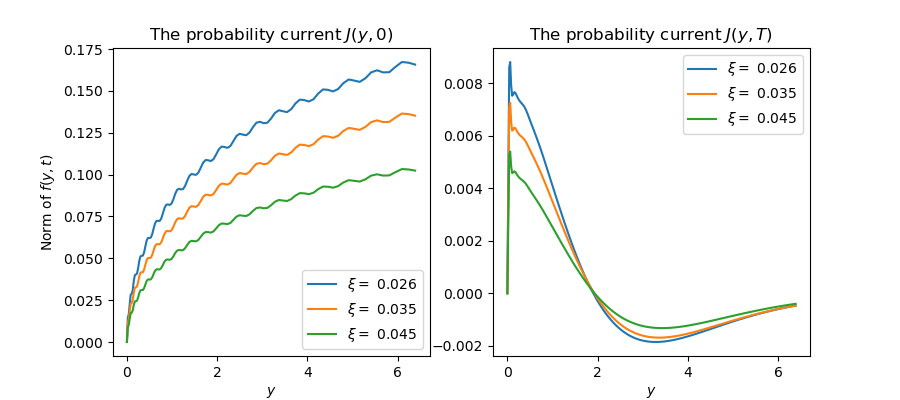
Figure 17: The probability current $J(y,t)$ according to Eq.(C.13) using $N=150$ basis functions. On the left: the initial probability current $J(y,0)$. On the right: $J(x,T)$ for $T=20$.

References

- [1] Abramowitz, M. and Stegun, I., Handbook of Mathematical Functions, Dover (1965).
- [2] Apanavicius, J., Feng, Y., Flores, Y., Hassan, M., and McGuigan, M., “Morse Potential on a Quantum Computer for Molecules and Supersymmetric Quantum Mechanics”, https://arxiv.org/abs/2102.05102 (2021).
- [3] Cooper, F., Khare, A., and Sukhatme, I., Supersymmetry in Quantum Mechanics, World Scientific (2001).
-
[4]
Das, S.R., Ostrov,D., Radhakrishnan, D., and Srivastav, D. “Dynamic Portfolio Allocation in Goal-Based Wealth Management”,
https://papers/ssrn.com/sol3/papers.cfm?abstractid=3211951 (2018). - [5] Dixon, M.F., Halperin, I., and Bilokon, P., Machine Learning in Finance: from Theory to Practice, Springer (2020).
- [6] Giet, J.S., Vallois, P., and Wantz-Mezieres, S., “The Logistic SDE”, Theory of Stochastic Processes, 20(36), 28-62 (2015).
- [7] Gradshteyn, I.S. and Ryzhik, I.M., Table of Integrals, Series, and Products, Seventh Edition, Academic Press (2007).
- [8] Halperin, I. “Non-Equilibrium Skewness, Market Crises, and Option Pricing: Non-linear Langevin Model of Markets with Supersymmetry”, Physica A, Volume 594, 15 May 2022, 127065, https://arxiv.org/abs/2011.01417 (2021).
- [9] Halperin, I. “Phases of MANES: Multi-Asset Non-Equilibrium Skew Model of a Strongly Non-Linear Market with Phase Transitions”, https://arxiv.org/abs/2203.07550 (2022).
- [10] Itkin, A., Lipton, A., and Muravey, D., “From the Black-Karasinski to the Verhulst model to accommodate the unconventional Fed’s policy”, https://arxiv.org/abs/2006.11976 (2021).
- [11] Itkin, A., Lipton, A., and Muravey, D.,, Generalized Integral Transforms in Mathematical Finance, World Scientific (2022).
- [12] Landau, L.D, and Lifschitz, E.M., Quantum Mechanics, 3rd Edition, Elsevier (1980).
- [13] Markowitz, H.M. ”Portfolio Selection”, The Journal of Finance, 7 (1), 77?91 (1952).
- [14] Merton, R.C., “Optimum Consumption and Portfolio Rules in a Continuous-Time Model”, Journal of Economic Theory, 3(4) 373-413 (1971).
- [15] Migdal, A.B., Qualitative Methods in Quantum Theory, W.A. Benjamin, Inc. Reading, MA (1977).
- [16] Molnar, B., Földi, P. Benedict, M.G., and Bartha, F., “Time Evolution in the Morse Potential Using Supersymmetry: Dissociation of the NO Molecule”, arXiv:quant-ph/0202069v1 (2002).
- [17] Simon, H.A. “A Behavioral Model of Rational Choice”, The Quarterly Journal of Economics, Vol. 69(1), 99-118 (1955).
- [18] Simon, H.A, “Rational Decision Making in Business Organizations”, The American Economic Review Vol. 69, No. 4, (1979).
- [19] Van Kampen, N.G., Stochastic Processes in Physics and Chemistry, North-Holland (1981).
- [20] Witten, E., ”Dynamical Breaking of Supersymmetry”, Nuclear Physics B 188(3-5), 513-554 (1981).