Deep evidential fusion with uncertainty quantification and contextual discounting for multimodal medical image segmentation

Abstract

Single-modality medical images generally do not contain enough information to reach an accurate and reliable diagnosis. For this reason, physicians generally diagnose diseases based on multimodal medical images such as, e.g., PET/CT. The effective fusion of multimodal information is essential to reach a reliable decision and explain how the decision is made as well. In this paper, we propose a fusion framework for multimodal medical image segmentation based on deep learning and the Dempster-Shafer theory of evidence. In this framework, the reliability of each single modality image when segmenting different objects is taken into account by a contextual discounting operation. The discounted pieces of evidence from each modality are then combined by Dempster’s rule to reach a final decision. Experimental results with a PET-CT dataset with lymphomas and a multi-MRI dataset with brain tumors show that our method outperforms the state-of-the-art methods in accuracy and reliability.

I Introduction

The advances in medical imaging machines and technologies now allow us to obtain multimodal medical images such as Positron Emission Tomography (PET)/Computed Tomography (CT) and multi-sequence Magnetic Resonance Imaging (MRI). Different modalities can provide complementary information about cancer and other abnormalities in the human body. Thus, the fusion of multiple sources of information is vital to improve the accuracy of diagnosis and to help radiotherapy. The success of information fusion depends on how well the fused knowledge represents reality [1]. More specifically, it depends on 1) how adequate the input information is, 2) how accurate and appropriate the prior knowledge is, and 3) the quality of the uncertainty model used [2].

Since the quality of input information and prior knowledge is usually out of control during the data analysis process, a trustworthy representation of uncertainty is desirable and should be considered as a key feature during the information fusion process. This is especially true in safety-critical application domains such as medical data analysis. Therefore, accurate multimodal medical image segmentation has to rely on an efficient model that is able to quantify segmentation uncertainty. Early approaches to quantify segmentation uncertainty are based on Bayesian theory [3]. In recent years, the popularity of deep segmentation models has revived research on model uncertainty estimation and has given rise to specific methods such as variational dropout [4] and deep ensembles [5]. However, as probabilistic segmentation models represent uncertainty using a single probability distribution, they cannot distinguish between aleatory and epistemic uncertainty, which limits the exploitation of the results.

The main task of multimodal medical image segmentation is to combine evidence from different modalities. Most existing fusion operators are based on optimistic assumptions about the reliability of the source of information and assume that they are equally reliable, which is not always true in reality. Therefore, the reliability coefficient of each source of information should be accounted for when doing fusion operations. Four major approaches can provide reliability coefficients: 1) modeling the reliability of sources using the degree of consensus[6]; 2) modeling expert opinions into possibility distribution [7]; 3) using external domain knowledge or contextual information to model reliability coefficient [8]; 4) learning the reliability coefficients by using training data in a neural network [9], which is the most general approach. Besides the reliability coefficient, the problem of the conflicts between sources remains as well. Though probabilistic approaches can combine information from different sources using techniques such as decision voting, they cannot effectively manage conflict when different decisions are assigned to the same input. Furthermore, probabilistic approaches can only model the corresponding weights instead of the reliability coefficients of each source information when combining multimodal evidence, limiting the fusion results’ performance and reliability.

In this paper, we explore a new approach that combines multimodal medical images based on the Dempster-Shafer theory (DST) of evidence [10, 11] and deep neural networks, where the segmentation uncertainty and reliability coefficients are first modeled and then taken into consideration when combining evidence from different sources. DST is a theoretical framework for modeling, reasoning with, and combining imperfect (imprecise, uncertain, and partial) information. With DST, we can quantify epistemic uncertainty directly and further explore the possibility of improving the model reliability based on the quantified uncertainty. Besides uncertainty quantification, DST offers a way to combine multiple unreliable information. Therefore we explore the possibility of studying an accurate and reliable multimodal medical image segmentation approach with contextual discounting under the framework of DST and deep neural networks . The idea of considering multimodal images as independent inputs and modeling the corresponding contributions or weights of each source information is simple. However, a reliable and explainable uncertainty quantification model is the theoretical guarantee to model the reliability coefficients of source information. Our method first computes mass functions to assign degrees of belief to each class and a degree of ignorance to the whole set of classes to represent segmentation uncertainty. It thus has one more degree of freedom than a probabilistic model, which allows us to model source uncertainty directly. Based on the quantified segmentation uncertainty, the reliability coefficients corresponding to each single modality input are modeled by a contextual discounting operation and be used for further operation. The main contributions of this paper are the following:

• For each single modality medical image, the segmentation uncertainty is modeled first, and the reliability coefficients when segmenting different contexts (tumors) are modeled using a contextual discounting operation as well.

• A multi-modality evidence fusion strategy is then applied to combine the discounted evidence from different modalities with DST by considering the conflicts and reliability.

• A complement evaluation of segmentation performance in both accuracy and reliability is conducted and a detailed analysis of the estimated reliability coefficient is provided to explain the segmentation results.

II Related work

II-A Dempster-Shafer theory

Let $\Theta=\{\theta_{1},\theta_{2},\ldots,\theta_{K}\}$ be a finite set of all possible hypotheses about some problem, called the frame of discernment. Evidence about a variable taking values in $\Theta$ can be represented by a mass function $m$, from the power set $2^{\Theta}$ to $[0,1]$, such that

$$\sum_{A\subseteq\Theta}m(A)=1,$$ (1a)

$$m(\emptyset)=0.$$ (1b)

Each subset $A\subseteq\Theta$ such $m(A)>0$ is called a focal set of $m$. The mass $m(A)$ represents a share of a unit mass of belief allocated to focal set $A$, which cannot be allocated to any strict subset of $A$. The mass $m(\Theta)$ represents the degree of ignorance about the problem, we can also call it the prediction uncertainty. Full ignorance is represented by a vacuous mass function $m_{\circ}$ verifying $m_{\circ}(\Theta)=1$. If all focal sets are singletons, then $m$ is said to be Bayesian and it is equivalent to a probability distribution.

II-A1 Belief and plausibility function

The information provided by a mass function $m$ can also be represented by a belief function $Bel$ or a plausibility function $Pl$ from $2^{\Theta}$ to $[0,1]$ defined, respectively, as:

$$Bel(A)=\sum_{B\subseteq A}m(B)$$ (2)

and

$$Pl(A)=\sum_{B\cap A\neq\emptyset}m(B)=1-Bel(\bar{A}),$$ (3)

for all $A\subseteq\Theta$, where $\bar{A}$ denotes the complement of $A$. The quantity $Bel(A)$ can be interpreted as a degree of support to $A$, while $Pl(A)$ can be interpreted as a measure of lack of support given to the complement of $A$. The contour function $pl$ associated to $m$ is the function that maps each element $\theta$ of $\Theta$ to its plausibility $Pl$:

$$pl(\theta)=Pl(\{\theta\}),\quad\forall\theta\in\Theta.$$ (4)

II-A2 Dempster’s rule

In DST, the belief about a certain question is elaborated by aggregating different belief functions over the same frame of discernment. Given two mass functions $m_{1}$ and $m_{2}$ derived from two independent pieces of evidence, the final belief that supports $A$ can be obtained by combining $m_{1}$ and $m_{2}$ with Dempster’s rule [11], denoted as $\oplus$, is formally defined by

$$(m_{1}\oplus m_{2})(A)=\frac{1}{1-\kappa}\sum_{B\cap C=A}m_{1}(B)m_{2}(C),$$ (5)

for all $A\subseteq\Theta,A\neq\emptyset$, and $(m_{1}\oplus m_{2})(\emptyset)=0$. The coefficient $\kappa$ is the degree of conflict between $m_{1}$ and $m_{2}$, with

$$\kappa=\sum_{B\cap C=\emptyset}m_{1}(B)m_{2}(C).$$ (6)

Mass functions $m_{1}$ and $m_{2}$ can be combined if and only if $\kappa<1$. The combined mass function $m_{1}\oplus m_{2}$ is called the orthogonal sum of $m_{1}$ and $m_{2}$. Let $pl_{1}$, $pl_{2}$ and $pl_{1}\oplus pl_{2}$ denote the contour functions associated with, respectively, $m_{1}$, $m_{2}$ and $m_{1}\oplus m_{2}$. The following equation holds:

$$pl_{1}\oplus pl_{2}(\theta)=\frac{pl_{1}(\theta)pl_{2}(\theta)}{1-\kappa}.$$ (7)

II-A3 Discounting operation

In the DST framework, the reliability of a source of information can be taken into account using the discounting operation, which transforms the evidence into a weaker, less informative one and thus allows for fusion with unreliable sources of information [11, 13, 14, 15]. Let $m$ be a mass function on $\Theta$ and $\beta$ a reliability coefficient in $[0,1]$. The discounting operation [11] with the discount rate $1-\beta$ transforms $m$ into:

$${}^{\beta}m=\beta\,m+(1-\beta)\,m_{\circ},$$ (8)

where $\beta$ is the degree of belief that the source mass function $m$ is reliable. When $\beta=1$, we accept the mass function $m$ provided by the source and take it as a description of our knowledge; when $\beta=0$, we reject it, and we are left with the vacuous mass function $m_{\circ}$. In [13], Mercier et al. extended the discounting operation with contextual discounting in the DST framework to refine the modeling of source reliability, which allows us to obtain more detailed information regarding the reliability of the source under different contexts, i.e., conditionally on different hypotheses regarding the variable of interest.

II-B DST-based evidential classifier

In [16], Denœux proposed a DST-based evidential neural network (ENN) classifier in which mass functions are computed based on distances to prototypes. Assuming we have several prototypes that represent information regarding inputs. The prototypes act as agents and provide us with independent evidence based on their domain knowledge. More specifically, the ENN considers each prototype as a piece of evidence, which is discounted based on its distance to the input vector. Here we provide a brief introduction to the ENN classifier. As shown in Figure 1, the ENN classifier comprises a prototype activation layer, a mass calculation layer, and a mass fusion layer.

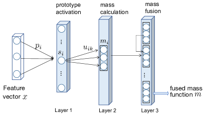
Figure 1: Evidential neural network

The prototype activation layer is composed of $I$ units, whose weight vectors are prototypes $p_{1},\ldots,p_{I}$ in input space. The activation of unit $I$ in the prototype layer is

$$s_{i}=\alpha_{i}\exp(-\gamma_{i}\left\|\boldsymbol{x}-\boldsymbol{p}_{i}\right\|^{2}),$$ (9)

$\gamma_{i}>0$ and $\alpha_{i}\in[0,1]$ are two parameters. For each prototype $\boldsymbol{p}_{i}$, the mass calculation layer computes mass functions $m_{i}$ that input $\boldsymbol{x}$ taking value in the frame of decrement $\Theta$, using the following equations:

$$m_{i}(\{\theta_{k}\}) =u_{ik}s_{i},\quad k=1,...,K$$ (10a)

$$m_{i}(\Theta) =1-s_{i},$$ (10b)

where $u_{ik}$ is the membership degree of prototype $p_{i}$ to class $\theta_{k}$, and $\sum_{k=1}^{K}u_{ik}=1$. Finally, the third layer combines the $I$ mass functions $m_{1},\ldots,m_{I}$ using Dempster’s rule (5). Tong et al. first applied ENN with convolutional neural network (CNN) in [17].

II-C Multimodal medical image segmentation

Using deep neural networks, researchers have mainly adopted probabilistic approaches to multimodal medical image segmentation. Probabilistic fusion strategies can be classified into image-level, feature-level, and decision-level fusion. For image-level fusion, multimodal images are concatenated by channels to construct a multi-channel input. For feature-level fusion, the multimodal images are taken as independent input at the beginning and then combined in the layers of the network by some concatenation strategies, such as attention mechanism [18]. For decision-level fusion, the multimodal medical images are taken as independent inputs to generate decisions and then are aggregated by averaging or majority voting. More details about probabilistic multimodal medical image segmentation can be found in [19].

Besides probabilistic approaches, some researchers focus on DST-based multimodal medical image segmentation. For example, George et al. proposed a breast cancer segmentation framework to transfer multiple CNN evidence into mass functions by using the discounting operation and then combined the discounted evidence using Dempster’s rule [20]. Apart from using discounting operations to generate mass functions, another solution is to construct deep evidential segmentation frameworks to output mass functions directly and then combine multiple pieces of evidence [21, 22]. More details about the DST-based multimodal medical image segmentation can be found in [23].

Though researchers have been devoted to the study of multimodal medical image segmentation approaches and have yielded promising experimental results, the question of the reliability of fused results and the theoretical explanation of why the fusion strategy is reliable still need to be studied. Thus, quantifying source reliability and combining the unreliable multimodal information is essential to reach a good segmentation result, as well as helping us to explain the results more convincingly. In this paper, we work on studying multimodal medical image segmentation with the deep evidential fusion framework by taking the uncertainty and reliability of multimodal medical images into consideration. More details about the proposed framework will be given in Section III.

III Proposed framework

The main idea of this work is to hybridize a deep evidential fusion framework with uncertainty quantification and contextual discounting for multimodal medical image segmentation. The proposed framework, shown in Figure  2, is composed of (1) several independent encoder-decoder feature extraction (FE) modules, (2) several independent evidential segmentation (ES) modules, and (3) a global multi-modality evidence fusion (MMEF) module.

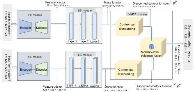
Figure 2: Deep evidential fusion framework. It is composed of encoder-decoder feature extraction (FE) modules that represent images using deep features, evidential segmentation (ES) modules that map deep features into mass functions, and a multimodal evidence fusion (MMEF) module that combines evidence from different modalities.

III-A Feature extraction (FE) module

The feature extraction module maps the input images into high-level deep representative features using deep neural networks. Since the focus of this paper is modeling the reliability of each source information and combing them reasonably to improve segmentation performance, we selected UNet [24], a basic medical image segmentation model, as our feature extraction module. The number of filters was set as $(8,16,32,64,128)$ with kernel size equal to five and convolutional strides equal to $(2,2,2,2)$ for layers from left to right. Our proposed framework could alternatively be applied to any state-of-the-art feature extraction models such as nnUNet [25]. Comparison and analysis of different feature extraction modules will be given in Section IV-C1.

III-B Evidential segmentation (ES) module

Based on the evidential classifier introduced in Section II-B, we proposed an ENN-based evidential segmentation module to segment voxel as well as quantify segmentation uncertainty about the class by mass functions. The basic idea of the evidential segmentation module is to assign each voxel the degrees of belief to the given classes and the degree of segmentation uncertainty based on the distance between the input $\boldsymbol{x}$ and $I$ prototypes. The input $\boldsymbol{x}$ is the high-level semantic deep feature vector generated by the feature extraction module. For each prototype $\boldsymbol{p}_{i}$, the evidential segmentation module first calculates an activate function $s_{i}$ using (9) in the prototype activation layer. Then a mass functions $m_{i}$ representing the corresponding evidence of prototype $\boldsymbol{p}_{i}$ is calculated by (10) in the mass calculation layer. Lastly, a final mass function $m$ is calculated in the mass fusion layer by combing the $I$ mass functions from $I$ prototypes using Demspter’s rule (5). As shown in Fig 2, for each input modality, we have an independent evidential segmentation module plugged into the feature extraction module’s output. For each voxel, the evidential segmentation module generates a mass value $m(\{\theta_{k}\})$ to each of the $K$ classes and a mass value $m(\Theta)$ to the whole set of classes $\Theta$. Here $m(\Theta)$ is the degree of ignorance when assigning a voxel to the given classes, representing segmentation uncertainty.

III-C Multi-modality evidence fusion (MMEF) module

In this section, we first explain the use of contextual discounting in quantifying the reliability of each source of information when segmenting different contexts. Then we introduce the combination of the discounted evidence from different modalities.

Discounting source evidence with reliability coefficients

As mentioned in Section II-A3, the reliability of source information can be modeled by the discounting operation. Furthermore, the reliability of a source of information in different contexts such as tumors can be modeled by contextual discounting. We followed Mercier’s idea [13] to extend the discounting operation into contextual discounting and model the reliability coefficient of each source modality when segmenting different kinds of tumors.

Assuming that we have evidence regarding the reliability of a source modality $t$, conditionally on each class $\theta_{k}\in\Theta$, i.e., in a context where the true class of $x$ is $\theta_{k}$. We thus have $K$ conditional mass functions ${}^{\beta^{t}_{k}}m^{t}(\{\theta_{k}\}),k=1,...,K$, instead of the single unconditional mass function ${}^{\beta^{t}}m^{t}$ in (8). Parameter ${\boldsymbol{\beta}}^{t}=[\beta^{t}_{1},\beta^{t}_{2},...,\beta^{t}_{k}]$ is a vector of the coefficient corresponding $K$ classes, $\beta^{t}_{k}$ represents our degree of belief that the modality $t$ is reliable when it is known that the actual value of $x$ is $\theta_{k}$, whereas $1-\beta^{t}_{k}$ represents the plausibility that the source information is not reliable under the same context. Let ${}^{{\boldsymbol{\beta}}^{t}}Pl^{t}$ be the plausibility function associate with mass function ${}^{{\boldsymbol{\beta}}^{t}}m^{t}$ for modality $t$, then the discounted plausibility function is defined as

$${}^{{\boldsymbol{\beta}}^{t}}Pl^{t}(A)=1-\prod_{\theta_{k}\in A}\beta^{t}_{k}\,(1-Pl^{t}(A))$$ (11)

for all $A\subset\Theta$, $k=1,...,K$. For each class $\theta_{k}$, the corresponding plausibility function can be represented as

$${}^{{\boldsymbol{\beta}}^{t}}Pl^{t}(\{\theta_{k}\}) =1-(1-Pl^{t}(\{\theta_{k}\}))\,\beta^{t}_{k}$$ (12a)

$$=1-\beta^{t}_{k}+Pl^{t}(\{\theta_{k}\})\,\beta^{t}_{k},\,k=1,...,K$$ (12b)

where ${}^{{\boldsymbol{\beta}}^{t}}Pl^{t}(\{\theta_{k}\})$ is the discounted plausibility of class $\theta_{k}$ from modality $t$, $Pl^{t}(\{\theta_{k}\})=pl^{t}(\theta_{k})=m^{t}(\{\theta_{k}\})+m^{t}(\Theta)$. We can decrease the calculation complexity by representing the evidence with the corresponding contour function. We thus use the discounted contour function ${}^{{\boldsymbol{\beta}}^{t}}pl^{t}$ instead of the discounted mass function ${}^{{\boldsymbol{\beta}}^{t}}m^{t}$ as our evidence for modality $t$ to simplify the computation.

Fusion with discounted evidence

The independent discounted evidence corresponding to different modalities should be combined reasonably to generate promising segmentation performance. Equation (7) allows us to compute the contour function in time proportional to the size of $\Theta$, without having to compute the combined mass $m_{1}\oplus m_{2}$ with (5). In our case, ${}^{{\boldsymbol{\beta}}^{t}}pl^{t}$ represent the discounted contour function provided, respectively, by modality $t$, with reliability vector ${\boldsymbol{\beta}}^{t}$. As a consequence of (7), the normalized contour function of multiple sources of information is proportional to the product of the contour function of each source of information. It can be used to simplify the processes of the orthogonal sum of $m_{1}$ and $m_{2}$ using Dempster’s rule. The predicted probability $P$ after combing evidence from $T$ modalities is, thus

$$P(\theta_{k})=\frac{\prod_{t=1}^{T}{{}^{\beta_{k}^{t}}}pl^{t}(\theta_{k})}{\sum_{k=1}^{K}\prod_{t=1}^{T}{{}^{\beta_{k}^{t}}}pl^{t}(\theta_{k})}$$ (13)

where $T$ is the number of input modalities, and $K$ is the number of classes on $\Theta$, $\beta_{k}^{t}$ is the reliability coefficient from modality $t$ that input taking value in class $\theta_{k}$.

III-D Loss function

The whole framework is trained by minimizing the Dice loss with respect to all network parameters and the reliability coefficients, given as follows:

$$loss_{D}=1-\frac{2\sum_{n=1}^{N}\sum_{k=1}^{K}{P_{kn}\times G_{kn}}}{\sum_{n=1}^{N}\sum_{k=1}^{K}{P_{kn}+G_{kn}}},$$ (14)

where $K$ and $N$ are the number of classes and voxels; $G_{kn}=1$ if voxel $n$ belongs to class $\theta_{k}$, and $G_{kn}=0$ otherwise, and $P_{kn}$ represents the corresponding predicted probabilities of voxel $n$ belongs to class $\theta_{k}$. In addition to learning the classifiers, the reliability coefficient $\beta^{t}_{k}$ corresponding to each modality $t$ and each class $\theta_{k}$ is learned.

IV Experiments and results

IV-A Experiment settings

IV-A1 Dataset

The proposed framework was tested on two multimodal medical image datasets: PET/CT lymphoma and multi-MRI brain tumor datasets.

The PET-CT lymphoma dataset considered in this paper contains 3D images from 173 patients who were diagnosed with large B-cell lymphomas and underwent PET-CT examination. The lymphomas in mask images were delineated manually by experts and considered as ground truth. The size and spatial resolution of PET and CT images and the corresponding mask images vary due to different imaging machines and operations. Figure 3 shows an example of a patient with lymphomas in PET and CT modality.

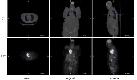
Figure 3: Example of a patient with lymphomas. The first and second rows show, respectively, CT and PET slices for one patient in axial, sagittal, and coronal views. The lymphomas correspond to the bright regions in PET slices.

The multi-MRI brain tumor dataset was offered by the BraTS2021 challenge [26]. The original BraTS2021 dataset comprises training, validation and test sets with the corresponding number of cases as 1251, 219 and 570, respectively. Each case has four modalities: FLAIR, T1Gd, T1 and T2 with $240\times 240\times 155$ voxels. Figure 4 shows examples of four modality MRI slices from one patient. The appearance of brain tumors varies in different modalities, and the tumor boundaries are blurred, making it hard to delineate different tumors precisely. Annotations of scans comprise the GD-enhancing tumor (ET-label 4), the peritumoral edema (ED-label 2), and the necrotic and non-enhancing tumor core (NRC/NET-label 1). The task of the BraTS2021 challenge is to segment three overlap regions: enhancing tumor (ET, label 4), tumor core (TC, the composition of label 1 and 4), and whole tumor (WT, the composition of label 1, 2, and 4).

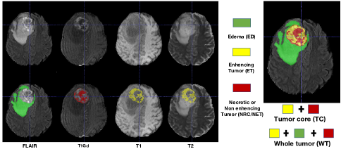
Figure 4: Examples of a patient with brain tumors in four modalities: Attenuated Inversion Recovery (FLAIR), post-contrast T1-weighted (T1Gd), native (T1) and T2-weighted (T2). The three tumor classes: enhancing core (yellow), necrotic/cystic core (red), and edema/invasion (green). The first, second and third columns show, respectively, the original image, the image with tumor mask in three classes (peritumoral edema(ED, green), enhancing tumor (ET, yellow), and necrotic tumor core or non-enhancing tumor (NCR/NET, red))

IV-A2 Pre-processing

For the PET-CT dataset, we first normalized the PET, CT and mask images: (1) for PET images, we applied a random intensity shift and scale of each channel with a shift value of 0 and scale value of 0.1; (2) for CT images, the shift and scale values were set to 1000 and 1/2000; (3) for mask images, the intensity value was normalized into the $[0,1]$ interval by replacing the outside value by $1$. We then resized the PET and CT images to $256\times 256\times 128$ by linear interpolation and resized mask images to $256\times 256\times 128$ by nearest neighbor interpolation. Lastly, registration of CT and PET images was performed by B-spline interpolation. Following [22], we randomly divided the 173 scans into 138, 17, and 18 for training, validation, and test set, respectively. The training process was then repeated five times to test the stability of our framework, with different data used exactly once as the validation and test data.

For the BraTS2021 dataset, we used the same pre-processing operation as in [27]. We first performed a min-max scaling operation followed by clipping intensity values to standardize all volumes, and then cropped/padded the volumes to a fixed size of $128\times 128\times 128$ by removing the unnecessary background (the cropped/padded operation is only applied for data used for training). No data augmentation technique was applied and no additional data was used in this study. Since the corresponding ground truth of the validation and test set is not available; thus, in this paper, we trained and tested our framework with the training set. Following [27], we randomly divided the 1251 training scans into 834, 208, and 209 for new training, validation, and test set, respectively. The training process was then repeated three times to test the stability of our framework. (We only repeated the training process three times to make sure different data were used exactly once as the validation and test data). All the prepossessing methods mentioned in this paper can be found in the SimpleITK [28] toolkit.

For all the compared methods, the same dataset composition and pre-processing operations were used. All methods were implemented based on the MONAI framework and can be called directly.

IV-A3 Parameter initialization and learning

The initial values of parameters (see (10)) $\alpha_{i}$ and $\gamma_{i}$ were set, respectively, to 0.5 and 0.01, and the membership degrees $u_{ik}$ were initialized randomly by drawing uniform random numbers, and normalizing. To simplify the framework, the prototypes $\boldsymbol{p}_{i}$ were initialized randomly from a normal distribution with zero mean and identity covariance matrix. Details about the initialization of the ES module can be found in the paper [22]. For the multimodal evidence fusion module, the initial value of reliability coefficient $\beta^{t}_{k}$ was set to 0.5. For the PET-CT and BraTS2021 datasets, each model was trained on the learning set with 100 epochs using the Adam optimization algorithm. The initial learning rate was set to $10^{-3}$. For all the compared methods, the model with the best performance on the validation set was saved as the final model for testing.

IV-A4 Evaluation criteria

In this paper, we evaluate the segmentation performance in its quality and reliability. The evaluation criteria used to assess the quality of medical image segmentation algorithms are Dice score, Sensitivity and Precision. These criteria are defined as follows:

$$\textsf{Dice}(P,T)=\frac{2\times TP}{FP+2\times TP+FN},$$

$$\textsf{Sensitivity}(P,T)=\frac{TP}{TP+FN},$$

$$\textsf{Precision}(P,T)=\frac{TP}{TP+FP},$$

where $TP$, $FP$, and $FN$ denote, respectively, the numbers of true positive, false positive, and false negative voxels.

In addition to the segmentation quality, the reliability of the segmentation results is also important. Therefore we use Brier score [29], negative log-likelihood (NLL) and Expected Calibration Error (ECE) [30] to evaluate the segmentation reliability. NLL evaluates the quality of model uncertainty with the definition

$$NLL=-\sum_{n=1}^{N}G_{n}log(P_{n})+(1-G_{n})log(1-P_{n}),$$

where $G_{n}$ is the ground truth of voxel $n$ and $P_{n}$ is the predicted probability of voxel $n$, $N$ is the number of voxels. Brier Score measures the accuracy of probabilistic predictions with the definition

$$BS=\frac{1}{N}\sum_{n=1}^{N}(P_{n}-G_{n})^{2},$$

where $G_{n}$ is the ground truth of voxel $n$ and $P_{n}$ is the predicted probability of voxel $n$, $N$ is the number of voxels. Expected Calibration Error (ECE) measures the correspondence between predicted probabilities and ground truth [30]. The output normalized plausibility of the model is first binned into equally spaced bin $E_{b}$, $b\in[1,B]$ ($B=10$ in this paper). The accuracy of bin $E_{b}$ is defined as

$$\textsf{acc}(E_{b})=\frac{1}{\mid E_{b}\mid}\sum_{n\in E_{b}}\boldsymbol{1}(S_{n}=G_{n}),$$

where $S_{n}$ and $G_{n}$ are, respectively, the predicted and true class labels for voxel $n$. The average confidence of bin $E_{b}$ is defined as

$$\textsf{conf}(E_{b})=\frac{1}{\mid E_{b}\mid}\sum_{n\in E_{b}}P_{n},$$

where $P_{n}$ is the predicted probability for voxel $n$. The ECE is the weighted average of the difference in accuracy and confidence of the bins:

$$ECE=\sum_{b=1}^{B}\frac{\mid E_{b}\mid}{N}\mid\textsf{acc}(E_{b})-\textsf{conf}(E_{b})\mid,$$

where $N$ is the total number of voxels in all bins, $\mid E_{b}\mid$ is the number of elements in bin $E_{b}$. A model is perfectly calibrated when $\textsf{acc}(E_{b})=\textsf{conf}(E_{b})$ for all $b\in\{1,...,B\}$.

Since our dataset has an imbalanced foreground and background proportion, thus, we only considered voxels belonging to the foreground or tumor region to calculate the NLL, Brier score and ECE. For the PET-CT lymphoma dataset, since the lymphomas are scattered throughout the whole body, focusing only on the tumor region is not easy. Thus, we focused on the foreground region for this dataset. For the BraTS2021 dataset, we followed the suggestion from [31] to focus on the tumor region for the reliability evaluation. For each patient in the test set, we defined a bounding box covering the foreground or tumor region and calculated the corresponding values in this bounding box. Similar to the other three segmentation performance criteria, the reported results were obtained by calculating each test 3D scan and then averaging over the patients.

IV-B Segmentation results on the PET-CT lymphoma dataset

IV-B1 Segmentation quality

We used the Dice Score, Sensitivity and Precision to evaluate the segmentation quality. We compared the performances of the MMEF-UNet with those of the baseline model, UNet [32], two state-of-the-art models, SegResNet [33] and nnUNet [25], as well as two evidential segmentation models, ENN-UNet and RBF-UNet [22]. Compared with UNet, SegResNet contains an additional variational autoencoder branch. NnUNet [25] is the first segmentation model designed as a segmentation pipeline for any given dataset by studying a recipe that systematizes the configuration process on a task-agnostic level. ENN-UNet and RBF-UNet are two DST-based deep evidential segmentation models that can calculate segmentation uncertainty directly. For nnUNet, the kernel size was set as $(3,(1,1,3),3,3)$ and the upsample kernel size was set as $(2,2,1)$ with strides $((1,1,1),2,2,1)$. For SegResNet [33], we used the pre-defined model without changing any parameter. We follow [22] to initialize the parameters of ENN-UNet and RBF-UNet. The same dataset composition and pre-processing operations were used for all the compared methods.

The comparison is shown in Table I. Compared with the baseline model UNet, our proposal MMEF-UNet greatly increases segmentation performance, e.g., a 3.5% increase in the Dice score. Compared with the two state-of-the-art segmentation methods, nnUNet and SegResNet, our proposal MMEF-UNet achieves the best segmentation performance in Dice score, Sensitivity and Precision. Compared with the two DST-based deep evidential segmentation methods, MMEF-UNet shows comparable segmentation performance. Figure 5 shows an example of visualized segmentation results obtained by UNet, ENN-UNet, RBF-UNet and MMEF-UNet. We can see that UNet and RBF-UNet are more conservative (they correctly detect only a subset of the tumor voxels) and ENN-UNet is more radical (some of the voxels that do not belong to tumors are predicted as tumors). However, the tumor regions predicted by MMEF-UNet better overlap the ground-truth tumor region, especially for the isolated lymphomas, which is also reflected by the promising Dice score and precision value.

TABLE I: Segmentation performance comparison on the lymphoma dataset. The bests and second bests are bold and underlined.

Model	Dice score $\uparrow$	Sensitivity $\uparrow$	Precision $\uparrow$
UNet [24]	0.770±0.070	0.891±0.043	0.893±0.034
nnUNet [25]	0.792±0.077	0.864±0.041	0.881±0.028
SegResNet [33]	0.798±0.091	0.901±0.058	0.886±0.046
ENN-UNet [22]	0.805±0.017	0.915±0.016	0.907±0.025
RBF-UNet [22]	0.802±0.016	0.913±0.015	0.905±0.021
MMEF-UNet (ours)	0.805±0.048	0.906±0.044	0.918±0.018

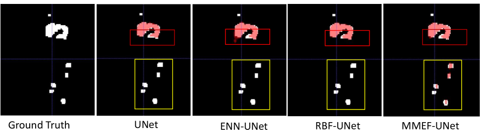
Figure 5: Examples of visualized segmentation results. From left to right, the ground truth and segmentation results obtained by UNet, ENN-UNet, RBF-UNet, and MMEF-UNet. The white and red regions represent, respectively, the ground truth and the segmentation result. Red and yellow boxes highlight the main differences in segmenting large and small isolated tumors.

IV-B2 Segmentation reliability

Although many researchers claimed that their approaches could improve the segmentation performance as a result of merging multimodal medical images into deep neural networks, the reliability of the results obtained with such fusion frameworks has seldom been investigated. There are two approaches to measuring segmentation reliability. One is to test the reliability of the model by calculating the quality of uncertainty quantification using criteria such as Brier score (IV-A4), NLL (IV-A4), and ECE (IV-A4). The other is to calculate the reliability of source information [34]. In this paper, the reliability of source information is represented by the reliability coefficients ${\boldsymbol{\beta}}$ we mentioned in (12b).

Deep ensembles [5] and Monte-Carlo (MC) dropout[4] are two popular techniques for improving the uncertainty quantification capabilities of probabilistic deep neural networks. We thus compared the ECE (IV-A4), Brier score and NLL achieved by UNet (the baseline model), UNet-MC (the baseline model with Monte-Carlo dropout), UNet-ensembles (the baseline model with deep ensembles), ENN-UNet and RBF-UNet (the uncertainty quantification methods), and our proposal MMEF-UNet. For UNet-MC, the dropout rate was set to 0.2 and the sample number was set to five; we averaged the five output probabilities at each voxel as the final output of the model. For UNet-ensembles, the sample number was set to five; the five output probabilities were then averaged at each voxel as the final output of the model.

Model’s reliability

The results concerning the model’s reliability are reported in Table II. We can see that Monte-Carlo dropout and deep ensembles enhance the segmentation quality (measured by the Dice score) of UNet, as well as improve the segmentation reliability (measured by the ECE, Brier score and NLL). Compared with UNet-MC and Unet-Ensembles, our proposal MMEF-UNet achieves the best segmentation performance. Compared to the two DST-based uncertainty quantification models, our proposal MMEF-UNet still shows priorities with higher segmentation quality and reliability.

TABLE II: Segmentation quality and reliability measures for MMEF-UNet and the referenced uncertainty quantification methods on the lymphoma dataset. The bests and second bests are bold and underlined.

Model	Dice score$\uparrow$	ECE $\downarrow$	Brier score $\downarrow$	NLL $\downarrow$
UNet	0.770±0.063	0.056±0.007	0.065±0.008	0.310±0.176
UNet-MC	0.801±0.023	0.053±0.009	0.062±0.010	0.400±0.174
UNet-Ensemble	0.802±0.015	0.063±0.015	0.064±0.008	0.343±0.144
ENN-UNet	0.805±0.009	0.050±0.007	0.062±0.008	0.191±0.027
RBF-UNet	0.802±0.014	0.051±0.007	0.061±0.002	0.193±0.027
MMEF-UNet	0.805±0.048	0.049±0.003	0.061±0.005	0.184±0.025

Reliability diagram

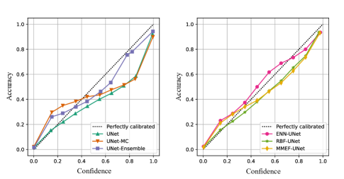
Figure 6: Calibration plots of difference deep segmentation models.

Figure 6 shows the calibration plots (also known as reliability diagrams) for the compared methods on the lymphoma dataset. The calibration plots compare how well the probabilistic predictions of a segmentation model are calibrated with its confidence matching its accuracy perfectly. The two probabilistic uncertainty quantification methods, UNet-MC and UNet-Ensemble, improve the calibration performance of UNet. Compared with the three probabilistic ones, the three DST-based models, ENN-UNet, RBF-UNet and MMEF-UNet (our proposal) have better calibration performance with their calibration curves closer to the perfected calibrated line. Among them, MMEF-UNet shows the best calibration performance as the calibration curve of ENN-UNet is almost overconfident and the calibration curve of RBF-UNet is almost underconfident.

Interpretation of reliability coefficients

The learned reliability coefficients of PET and CT when segmenting lymphomas are 0.99 and 0.97, which means the information from the PET modality is more reliable than the CT modality when segmenting lymphomas. This information is consistent with the domain knowledge that PET images provide functional information about tumor activity and usually be used to locate tumors, and CT images provide anatomic information and always be used as a complement to PET for radiotherapy.

IV-C Segmentation results on the multi-MRI BrsTS2021 dataset

IV-C1 Segmentation quality

For the BraTS2021 dataset, we first test the segmentation performance on MMEF-UNet. Then we took nnUNet as another feature extraction module and constructed a deep evidential fusion framework, named MMEF-nnUNet, because nnUNet is reported to be the best-performed segmentation model in BraTS2021 challenge [35]. Thus we compared our results with two baseline models (UNet and nnUNet), one classical CNN-based method (V-Net [36]), and one DST-based evidential segmentation model (ENN-UNet [22]) in Table III. MMEF-UNet outperforms the above-mentioned segmentation models in terms of the three overlapped regions, ET, TC and WT, as well as in the mean Dice score.

TABLE III: Segmentation performance comparison on the BraTS2021 dataset. The bests and second bests are bold and underlined.

Methods	Dice score $\uparrow$
	ET	TC	WT	Mean
UNet [24]	0.801±0.021	0.824±0.019	0.876±0.017	0.834±0.018
VNet [36]	0.788±0.029	0.851±0.038	0.905±0.096	0.848±0.054
nnUNet [25]	0.796±0.012	0.857±0.014	0.915 ±0.010	0.856±0.011
ENN-UNet [22]	0.801±0.023	0.830±0.024	0.896±0.014	0.843±0.020
MMEF-UNet (Ours)	0.803±0.027	0.839±0.005	0.904±0.008	0.848±0.009
MMEF-nnUNet (Ours)	0.800±0.012	0.856±0.004	0.920±0.009	0.859±0.006

IV-C2 Segmentation reliability

Model’s reliability

Similar to the lymphoma dataset, for the BrsTs2021 dataset, we also calculated ECE, Brier score and NLL, to test the segmentation reliability. Applying deep ensembles for larger-scale datasets, e.g., BraTS2021, requires high computation capacity and is time-consuming. Thus, for the BraTS2021 dataset, we only calculated the results of applying Monte-Carlo dropout with UNet and nnUNet, named UNet-MC and nnUNet-MC. The comparisons are shown in Table IV. The best segmentation quality and reliability are achieved by MMEF-nnUNet, with the highest Dice score of 0.859; the lowest ECE, Brier and NLL values, 0.051, 0.103 and 1.784, respectively.

TABLE IV: Segmentation quality and reliability measures for MMEF-UNet, MMEF-nnUNet and the reference methods on the BraTS2021 dataset. The bests and second bests are bold and underlined.

Model	Dice score $\uparrow$	ECE $\downarrow$	Brier score $\downarrow$	NLL $\downarrow$
UNet	0.833±0.014	0.072±0.002	0.143±0.004	2.476±0.061
UNet-MC	0.841±0.005	0.065±0.004	0.133±0.011	2.266±0.164
MMEF-UNet	0.848±0.009	0.064±0.003	0.128±0.005	2.209±0.091
nnUNet	0.851±0.008	0.052±0.004	0.108±0.010	1.867±0.183
nnUNet-MC	0.855±0.009	0.053±0.004	0.109±0.011	1.820±0.133
MMEF-nnUNet	0.859±0.006	0.051±0.004	0.103±0.007	1.784 ±0.132

Interpretation of reliability coefficients

Table V and VI show the learned reliability coefficients ${\boldsymbol{\beta}}$ (see (12b)), estimated by MMEF-UNet and MMEF-nnUNet, respectively, for the four modalities with three different tumor classes. In Table V, the evidence from the T1Gd modality is reliable when segmenting ED, ET, and NRC/NET classes, with all the reliability values greater than 0.9. In contrast, the evidence from the FLAIR modality is more reliable for the ED class as the reliability values in ET and NRC/NET are less than 0.9. The evidence from the T1 modality is less reliable compared with the other three modalities, e.g., the reliability value when segmenting the ED class is less than 0.5. There are small differences between Table V and VI while their general tendency is similar. The differences between the two tables are also interesting, e.g., the reliability coefficient for the T1Gd modality from MMEF-nnUNet is higher than that of MMEF-UNet, which can be attributed to a better feature extraction ability of nnUNet. According to the above summary, we can conclude that there are two approaches to addressing the imperfect (unreliable or noisy) source information: either work on better feature representation algorithms or work on evidence-discounting algorithms to eliminate the negative effect of the imperfect information.

Furthermore, those reliability results from Table V and VI are consistent with domain knowledge about these modalities reported in [26], i.e., the appearance of NRC/NET is hypointense on the T1Gd modality; ED is defined by the abnormal hyperintense signal on the FLAIR modality. That explains why the corresponding reliability coefficient is high for those regions. This interpretation of the reliability coefficient offers a way to explain the segmentation results to physicians and patients as well.

TABLE V: Estimated reliability coefficient ${\boldsymbol{\beta}}$ (after training) of UNet for classes ET, ED and NRC/NET in the four modalities. Higher values correspond to greater contribution to the segmentation.

${\boldsymbol{\beta}}$		ED	ET	NRC/NET
T1Gd		0.999±0.003	0.949±0.086	0.923±0.131
FLAIR		0.922±0.094	0.852±0.054	0.895±0.056
T1		0.480±0.261	0.790±0.160	0.824±0.009
T2		0.848±0.064	0.785±0.096	0.890±0.009

TABLE VI: Estimated reliability coefficients ${\boldsymbol{\beta}}$ (after training) of nnUNet for classes ED, ET, and NRC/NET in the four modalities. Higher values correspond to greater contribution to the segmentation.

${\boldsymbol{\beta}}$		ED	ET	NRC/NET
T1Gd		0.997±0.003	0.997±0.001	0.991±0.005
FLAIR		0.947±0.008	0.697±0.060	0.797±0.045
T1		0.736±0.066	0.763±0.025	0.827±0.068
T2		0.804±0.128	0.814±0.040	0.921±0.039

IV-D Ablation analysis

We also investigated the contribution of each module to the whole framework’s performance. Table VII highlights the importance of introducing the evidential segmentation and multimodal evidence fusion modules. UNet is the baseline model that uses the softmax transformation to map feature vectors into probabilities; UNet-ES uses the evidential segmentation instead of softmax to map feature vectors into mass functions and uses pignistic transformation [37] to get segmentation probabilities; MMEF-UNet is our final proposal.

TABLE VII: Segmentation quality and reliability under different input modality and fusion strategies.

Module components	Input modality	Dice score $\uparrow$	Sensitivity $\uparrow$	Precision $\uparrow$	ECE $\downarrow$	Brier score $\downarrow$	NLL $\downarrow$
UNet+softmax	CT	0.544±0.062	0.789±0.041	0.794±0.021	0.133±0.011	0.157±0.022	0.571±0.0817
	PET	0.764±0.066	0.901±0.042	0.883±0.033	0.060±0.009	0.068±0.009	0.348±0.183
	PET+CT	0.770±0.070	0.893±0.046	0.0893±0.035	0.056±0.008	0.065±0.008	0.309±0.197
UNet+ES	CT	0.543±0.061	0.787±0.043	0.795±0.021	0.131±0.019	0.156±0.023	0.521±0.072
	PET	0.781±0.079	0.892±0.040	0.903±0.041	0.050±0.011	0.064±0.012	0.195±0.050
UNet+ES+MMEF	PET+CT	0.805±0.054	0.906±0.044	0.918±0.018	0.049±0.003	0.061±0.005	0.184±0.025

IV-D1 Effectiveness of uncertainty quantification

Table VII shows the performance with and without the evidential segmentation module when only PET or CT images are used. Compared with the baseline method UNet, our proposal, which plugs the evidential segmentation module after UNet, improves the segmentation performance when single modality images are used. For example, compared with UNet, UNet-ES has an increase of 1.7% and 1%, respectively, in Dice score and Precision when using PET images. Furthermore, the introduction of evidential segmentation improves the reliability of the segmentation results, e.g., a decrease of 12.5% in NLL.

IV-D2 Effectiveness of multimodal evidence fusion with contextual discounting

We also tested the segmentation performance of two fusion approaches, UNet with image concatenation and MMEF-UNet with evidence fusion, when both PET and CT are used as input. As shown in Table VII, it is not surprising that the fusion of PET and CT images shows better segmentation performance than single modality (PET or CT) images, e.g., the introduction of MMEF has an increase of 4.1% and 26.1% in the Dice score compared with single PET and CT input. The segmentation performance on Sensitivity and Precision also yields similar priorities of the two multimodal fusion methods. Compared with image concatenation, multimodal evidence fusion with contextual discounting improves the segmentation quality with a higher Dice score. As for segmentation reliability, MMEF-UNet has the smallest ECE, Brier score and NLL, which yields the most reliable segmentation performance.

V Conclusion

Based on DST, a deep evidential fusion framework with uncertainty quantification and contextual discounting is proposed for multimodal medical image segmentation. The segmentation uncertainty is quantified directly by an evidential segmentation module that calculates the uncertainty when classifying a voxel into given classes. The multimodal evidence fusion module first models the reliability of each modality information when segmenting different tumors with contextual discounting and then combines the discounted multimodal evidence with Dempster’s rule. To our best knowledge, this approach is the first attempt to apply evidence theory with contextual discounting to the fusion of deep neural networks and apply it to multimodal medical image segmentation tasks. Our method can be considered a decision-level fusion method and can be used with any state-of-the-art feature extraction module for different tasks.

In future research, refining the framework to improve its segmentation performance and reduce complexity will be considered. Another interesting research direction, accordingly, is to estimate task-specific reliability and enhance the explainability of deep evidential neural networks on different medical datasets. Furthermore, the application of our framework for cross-modality biomedical information analysis tasks, e.g., signals, images, biomedical indicators, and gene information, is also an interesting research direction.

VI Biography Section

Ling Huang received her Ph.D. degree in Computer Science student from the University of Technology of Compiegne, France, in 2023. Her research interests include machine learning, information fusion, uncertainty quantification and medical data analysis.

Su Ruan received her Ph.D. degree in Image Processing from the University of Rennes, France, in 1993. Her research interests include pattern recognition, machine learning, information fusion, and medical imaging.

Pierre Decazes is currently a nuclear medicine physician from Henri Becquerel Cancer Center and Rouen University.

Thierry Denœux is a Full Professor (Exceptional Class) with the Department of Information Processing Engineering at the University of Technology of Compiegne, France, and a senior member of the French Academic Institute (Institut Universitaire de France). His research interests concern reasoning and decision-making under uncertainty and, more generally, the management of uncertainty in intelligent systems.

References

- [1] F. E. White, “Data fusion lexicon,” Joint Directors of Labs Washington DC, Tech. Rep., 1991.
- [2] G. L. Rogova and V. Nimier, “Reliability in information fusion: literature survey,” in Proceedings of the seventh international conference on information fusion, vol. 2, 2004, pp. 1158–1165.
- [3] G. E. Hinton and D. Van Camp, “Keeping the neural networks simple by minimizing the description length of the weights,” in Proceedings of the sixth annual conference on Computational learning theory, 1993, pp. 5–13.
- [4] Y. Gal and Z. Ghahramani, “Dropout as a bayesian approximation: Representing model uncertainty in deep learning,” in international conference on machine learning. PMLR, 2016, pp. 1050–1059.
- [5] B. Lakshminarayanan, A. Pritzel, and C. Blundell, “Simple and scalable predictive uncertainty estimation using deep ensembles,” Advances in neural information processing systems, vol. 30, 2017.
- [6] F. Delmotte, L. Dubois, and P. Borne, “Context-dependent trust in data fusion within the possibility theory,” in 1996 IEEE International Conference on Systems, Man and Cybernetics. Information Intelligence and Systems (Cat. No. 96CH35929), vol. 1. IEEE, 1996, pp. 538–543.
- [7] R. Cooke et al., Experts in uncertainty: opinion and subjective probability in science. Oxford University Press on Demand, 1991.
- [8] S. Fabre, A. Appriou, and X. Briottet, “Presentation and description of two classification methods using data fusion based on sensor management,” Information Fusion, vol. 2, no. 1, pp. 49–71, 2001.
- [9] Z. Elouedi, K. Mellouli, and P. Smets, “Assessing sensor reliability for multisensor data fusion within the transferable belief model,” IEEE Transactions on Systems, Man, and Cybernetics, Part B (Cybernetics), vol. 34, no. 1, pp. 782–787, 2004.
- [10] A. P. Dempster, “Upper and lower probability inferences based on a sample from a finite univariate population,” Biometrika, vol. 54, no. 3-4, pp. 515–528, 1967.
- [11] G. Shafer, A mathematical theory of evidence. Princeton University Press, 1976, vol. 42.
- [12] L. Huang, T. Denoeux, P. Vera, and S. Ruan, “Evidence fusion with contextual discounting for multi-modality medical image segmentation,” in Medical Image Computing and Computer Assisted Intervention–MICCAI 2022: 25th International Conference, Singapore, September 18–22, 2022, Proceedings, Part V. Springer, 2022, pp. 401–411.
- [13] D. Mercier, B. Quost, and T. Denœux, “Refined modeling of sensor reliability in the belief function framework using contextual discounting,” Information fusion, vol. 9, no. 2, pp. 246–258, 2008.
- [14] D. Mercier, É. Lefevre, and F. Delmotte, “Belief functions contextual discounting and canonical decompositions,” International Journal of Approximate Reasoning, vol. 53, no. 2, pp. 146–158, 2012.
- [15] F. Pichon, D. Mercier, É. Lefevre, and F. Delmotte, “Proposition and learning of some belief function contextual correction mechanisms,” International Journal of Approximate Reasoning, vol. 72, pp. 4–42, 2016.
- [16] T. Denœux, “A neural network classifier based on Dempster-Shafer theory,” IEEE Transactions on Systems, Man, and Cybernetics-Part A: Systems and Humans, vol. 30, no. 2, pp. 131–150, 2000.
- [17] Z. Tong, P. Xu, and T. Denoeux, “An evidential classifier based on dempster-shafer theory and deep learning,” Neurocomputing, vol. 450, pp. 275–293, 2021.
- [18] T. Zhou, S. Ruan, P. Vera, and S. Canu, “A tri-attention fusion guided multi-modal segmentation network,” Pattern Recognition, vol. 124, p. 108417, 2022.
- [19] T. Zhou, S. Ruan, and S. Canu, “A review: Deep learning for medical image segmentation using multi-modality fusion,” Array, vol. 3, p. 100004, 2019.
- [20] K. George, S. Faziludeen, and P. Sankaran, “Breast cancer detection from biopsy images using nucleus guided transfer learning and belief based fusion,” Computers in Biology and Medicine, vol. 124, p. 103954, 2020.
- [21] L. Huang, S. Ruan, and T. Denœux, “Belief function-based semi-supervised learning for brain tumor segmentation,” in 2021 IEEE 18th International Symposium on Biomedical Imaging (ISBI). IEEE, 2021, pp. 160–164.
- [22] L. Huang, S. Ruan, P. Decazes, and T. Denœux, “Lymphoma segmentation from 3d pet-ct images using a deep evidential network,” International Journal of Approximate Reasoning, vol. 149, pp. 39–60, 2022.
- [23] L. Huang, S. Ruan, and T. Denoeux, “Application of belief functions to medical image segmentation: A review,” Information fusion, vol. 91, pp. 737–756, 2023.
- [24] E. Kerfoot, J. Clough, I. Oksuz, J. Lee, A. P. King, and J. A. Schnabel, “Left-ventricle quantification using residual u-net,” in International Workshop on Statistical Atlases and Computational Models of the Heart. Springer, 2018, pp. 371–380.
- [25] F. Isensee, J. Petersen, A. Klein, D. Zimmerer, P. F. Jaeger, S. Kohl, J. Wasserthal, G. Koehler, T. Norajitra, S. Wirkert et al., “nnu-net: Self-adapting framework for u-net-based medical image segmentation,” arXiv preprint arXiv:1809.10486, 2018.
- [26] U. Baid, S. Ghodasara, S. Mohan, M. Bilello, E. Calabrese, E. Colak, K. Farahani, J. Kalpathy-Cramer, F. C. Kitamura, S. Pati et al., “The rsna-asnr-miccai brats 2021 benchmark on brain tumor segmentation and radiogenomic classification,” arXiv preprint arXiv:2107.02314, 2021.
- [27] H. Peiris, M. Hayat, Z. Chen, G. Egan, and M. Harandi, “A robust volumetric transformer for accurate 3d tumor segmentation,” in Medical Image Computing and Computer Assisted Intervention–MICCAI 2022: 25th International Conference, Singapore, September 18–22, 2022, Proceedings, Part V. Springer, 2022, pp. 162–172.
- [28] B. C. Lowekamp, D. T. Chen, L. Ibáñez, and D. Blezek, “The design of simpleitk,” Frontiers in neuroinformatics, vol. 7, p. 45, 2013.
- [29] G. W. Brier et al., “Verification of forecasts expressed in terms of probability,” Monthly weather review, vol. 78, no. 1, pp. 1–3, 1950.
- [30] C. Guo, G. Pleiss, Y. Sun, and K. Q. Weinberger, “On calibration of modern neural networks,” in International Conference on Machine Learning. PMLR, 2017, pp. 1321–1330.
- [31] A.-J. Rousseau, T. Becker, J. Bertels, M. B. Blaschko, and D. Valkenborg, “Post training uncertainty calibration of deep networks for medical image segmentation,” in 2021 IEEE 18th International Symposium on Biomedical Imaging (ISBI). IEEE, 2021, pp. 1052–1056.
- [32] O. Ronneberger, P. Fischer, and T.-n. Brox, “Convolutional networks for biomedical image segmentation,” in International Conference on Medical Image Computing and Computer-Assisted Intervention, Munich, Germany, Oct, 2015.
- [33] A. Myronenko, “3d mri brain tumor segmentation using autoencoder regularization,” in International MICCAI Brainlesion Workshop. Springer, 2018, pp. 311–320.
- [34] F. Kobayashi, F. Arai, and T. Fukuda, “Sensor selection by reliability based on possibility measure,” in Proceedings 1999 IEEE International Conference on Robotics and Automation (Cat. No. 99CH36288C), vol. 4. IEEE, 1999, pp. 2614–2619.
- [35] H. M. Luu and S.-H. Park, “Extending nn-unet for brain tumor segmentation,” in Brainlesion: Glioma, Multiple Sclerosis, Stroke and Traumatic Brain Injuries. Cham: Springer International Publishing, 2022, pp. 173–186.
- [36] F. Milletari, N. Navab, and S.-A. Ahmadi, “V-net: Fully convolutional neural networks for volumetric medical image segmentation,” in 2016 fourth international conference on 3D vision. IEEE, 2016, pp. 565–571.
- [37] P. Smets and R. Kennes, “The transferable belief model,” Classic Works of the Dempster-Shafer Theory of Belief Functions, pp. 693–736, 2008.