C=Anything and the switchback effect in
Schwarzschild-de Sitter space

Abstract

We investigate observables within the framework of the codimension-one C=Anything (CAny) proposal for Schwarzschild-de Sitter (SdS) space under the influence of shockwave sources. Within the proposal, there is a set of time-reversal invariant observables that display the same rate of growth at early and late times for a background with or without shockwave sources. Once we introduce shockwaves in the weak gravitational coupling regime, there is a decrease in the late-time complexity growth due to cancellations with early-time perturbations, known as the switchback effect. The result shows that some CAny observables in SdS may reproduce the same type of behavior found in anti-de Sitter black holes. We comment on how our results might guide us to new explorations in the putative quantum mechanical theory.

1 Introduction

Recently, a lot of interest in quantum information theoretic notions has surfaced in an effort to characterize semiclassical gravitational observables. Particularly, holographic complexity has been used to study bulk gravitational dynamics that can probe regions inaccessible to entanglement entropy Susskind:2014moa ; Susskind:2014rva ; Stanford:2014jda , and whose variation can also reproduce gravitational equations of motion Czech:2017ryf ; Caputa:2018kdj ; Susskind:2019ddc ; Pedraza:2021mkh ; Pedraza:2021fgp ; Pedraza:2022dqi . This notion is also expected to reproduce the properties for the computational complexity of a quantum circuit model of the conformal field theory (CFT) dual to asymptotically Anti-de Sitter (AdS) spacetimes Susskind:2014rva . This translates to robust features captured by a large family of proposals, starting with the Complexity=Volume (CV) Stanford:2014jda , Complexity=Action (CA) Brown:2015bva ; Brown:2015lvg , Complexity=Spacetime Volume (CV2.0) Couch:2016exn , and a recent generalization known as the Complexity=Anything (CAny) proposal Belin:2021bga ; Belin:2022xmt . There are two defining features for the CAny observables in AdS black holes: (i) a late boundary time linear growth, and (ii) the switchback effect. The latter is a characteristic decrease in the late-time linear growth once perturbations in the geometry are introduced due to energy pulses.

Perhaps, one of the most exciting aspects about this family of spacetime probes is to characterize the properties of cosmological backgrounds, and in particular for de Sitter (dS) space. The nature of the microscopic degrees of freedom encoded inside the cosmological horizon remains mysterious (see Galante:2023uyf for a recent review).

A recent proposal in dS holography, known as stretched horizon holography Susskind:2021esx ; Shaghoulian:2022fop ; Susskind:2022dfz ; Lin:2022rbf ; Lin:2022nss ; Bhattacharjee:2022ave ; Rahman:2022jsf ; Susskind:2023hnj ; Susskind:2023rxm ; Franken:2023pni ; Lin:2023trc , has sparked many developments in dS space complexity. The stretched horizon is a region in the static patch of dS space where the dual theory is conjectured to be located Susskind:2021esx . One may therefore perform gravitational dressings with respect to the stretched horizon to probe the dual degrees of freedom. Although the precise location is not explicit in this approach, it is expected to be close to the cosmological horizon. This approach has been explored to study holographic complexity proposals in asymptotically dS space Jorstad:2022mls ; Auzzi:2023qbm ; Anegawa:2023dad ; Baiguera:2023tpt ; Anegawa:2023wrk ; Aguilar-Gutierrez:2023zqm ; Aguilar-Gutierrez:2023tic . One of the striking features originally found in Jorstad:2022mls for the CV, CA, and CV2.0 proposals was that the rate of growth of holographic complexity might diverge a finite times relative to the stretched horizon, denoted by hyperfast growth. The result was associated with the conjecture where the double-scaled Sachdev–Ye–Kitaev (SYK) model is identified as the quantum mechanical dual to dS₂ space Susskind:2021esx . One may introduce a cutoff surface to perform an analytic continuation allowing for late-time evolution Jorstad:2022mls .

However, it was recently found that hyperfast growth is not a universal phenomenon in the space of holographic complexity proposals Aguilar-Gutierrez:2023zqm . Instead, a set of the CAny observables may evolve to arbitrarily late (or early) static patch times without introducing regulator surfaces. Notice, however, that it is still unclear what kind of interpretation the different types of CAny observables might have for dS space. To properly define holographic complexity proposals one needs a good understanding of the basic properties that complexity for the dual field theory side should satisfy. Such understanding of the microscopics associated with dS space is still lacking. It is important to learn about the different signals one should look for in a candidate for the dS space holographic model.

Alternatively, one might find clearer interpretations of holographic complexity when dS space is embedded in a higher dimensional bulk AdS spacetime. This perspective was recently approached by Aguilar-Gutierrez:2023tic . They considered a particular type of CAny proposals in a braneworld model consisting of a higher dimensional AdS bulk geometry capped off by a pair of dS space end-of-the-world branes. In this setting, the resulting complexity is associated with the field theory dual living on a brane near the asymptotic boundary of the AdS space. In this case, the CAny proposals with the expected late time growth in the AdS bulk are those that obey the late time growth in the dS braneworld.

On the other hand, one of the defining properties of holographic complexity proposals in the AdS context, the switchback effect, has been recently explored in asymptotically dS spacetime Anegawa:2023wrk ; Baiguera:2023tpt for the CV, CA, CV2.0 proposals. In this case, there are energy pulses associated with perturbations in the evolution of the putative dual theory residing in the stretched horizon. This can be an important diagnostic if the CAny observables can indeed be associated with complexity consistent with Nielsen’s geometric approach in the dual theory Aguilar-Gutierrez:2023zqm . However, the switchback effect in the class of CAny observables where the late-time growth in dS space is allowed has not been studied. This is the main goal of our work, to learn new lessons for stretched horizon holography.

To study the switchback effect, we describe the shockwave geometry in asymptotically dS spacetimes. We specialize in Schwazschild-de Sitter (SdS) space, which describes spherically symmetric vacuum solutions to Einstein equations with a positive cosmological constant. We work in the perturbative weak gravity regime to treat the shockwave geometry based on previous findings in Shenker:2013pqa , and recently discussed in the context of SdS black holes by Aguilar-Gutierrez:2023ymx . As for the observables, we will work with codimension-one CAny proposals evaluated in constant mean curvature (CMC) slices, originally introduced in Belin:2022xmt . The mean curvature is one of the main factors distinguishing the proposals that display late time growth from those with hyperfast growth Aguilar-Gutierrez:2023zqm .

Our work is focused on alternating early and late-time perturbations in the geometry and the resulting growth of the CAny observables. Our findings indicate that the set of proposals with late-time growth will display the switchback effect. The rate of growth will be determined by the definition of the CAny proposal. In general, however, the manifestation of the switchback effect in the CAny proposals only occurs once we perform a time-reversal symmetric extension, originally hinted in Aguilar-Gutierrez:2021bns . We select CMC slices that minimize the CAny proposal and find that the late-time and early-time contributions to complexity growth will partially cancel out. Under these conditions, the analysis of the switchback effect shows great similarity with respect to that of AdS black hole backgrounds.

Interestingly, the late time growth during the switchback phase is unaffected by the particular location of the stretched horizon.

The structure of the manuscript goes as follows. In Sec. 2 we review generalities about the shockwave geometries in SdS spacetimes, as well as the CAny proposals that display the early and late-time growth in SdS spacetime. We introduce some new results regarding the generalizing the set of proposals that reproduce the late time growth of complexity in SdS space of arbitrary mass (below the extremal one). In Sec. 3, we present the results on the switchback effect in SdS spacetime by performing a series of alternating shockwave insertions in the background geometry in the weak gravity regime. Finally, Sec. 4 includes a summary of our findings in this setting and some interesting directions for future research. For the convenience of the reader, we provide an App. A containing some of the details about the evaluation of the late-time growth of the CAny proposals.

2 C=Anything in SdS spacetimes

In this section, we briefly review basic notions about SdS_d+1 black holes, the modification in the geometry due to shockwave insertions, and the CAny proposals that we investigate in this work. New results include extending the set of CAny proposals studied in Aguilar-Gutierrez:2023zqm for SdS space, to more general observables than volumes of CMC slices. This allows for different types of late-time growth behaviors in $d=2$, $d=3$. We also show that late-time growth persists for arbitrary mass black holes.

2.1 SdS spacetimes

The configuration of interest is SdS_d+1 space, described by the line element

$$\mathrm{d}s^{2} =-f(r)\mathrm{d}t_{L/R}^{2}+\frac{\mathrm{d}r^{2}}{f(r)}+r^{2}\mathrm{d}\Omega_{d-1}^{2}\,,$$ (1)

$$f(r) =1-\frac{r^{2}}{\ell^{2}}-\frac{2\mu}{r^{d-2}}\leavevmode\nobreak\ ,\quad\mu\equiv\frac{16\pi G_{N}M}{(d-1)\Omega_{d-1}r^{d-2}}\leavevmode\nobreak\ ,$$ (2)

with $\ell^{2}=d(d-1)/(2\Lambda)$; $\Lambda>0$ is the cosmological constant; $M$ parametrizes the mass of the black hole; $G_{N}$ is Newton’s constant; $\Omega_{d-1}=2\pi^{d/2}/\Gamma(d/2)$ is the volume of a unit ($d-1$)-sphere; $\mu\in[0,\,\mu_{N}]$. The case where $\mu=\mu_{N}$, with

$$\mu_{N}=\frac{1}{d}\quantity(\frac{d-2}{d})^{\frac{d-2}{2}}\leavevmode\nobreak\ ,$$ (3)

describes the most massive black hole supported in dS space, which we refer to as the extremal SdS limit. Meanwhile, $\mu=0$, reproduces dS_d+1 space.

We will be interested in describing shockwaves in the geometry. It’s convenient to use Kruskal coordinates, defined by

$$U_{\rm b,\rm c} =\mathrm{e}^{\frac{f^{\prime}(r_{\rm b,\rm c})}{2}\left(r_{*}(r)-t\right)}\leavevmode\nobreak\ ,$$ (4)

$$V_{\rm b,\rm c} =-\mathrm{e}^{\frac{f^{\prime}(r_{\rm b,\rm c})}{2}\left(r_{*}(r)+t\right)}\,.$$

where the subindices “b, c” denote coordinates on the black hole and inflating patches. These patches are centered at the horizons $r_{\rm b,\rm c}$, and cover the range $0\leq r<r_{\mathcal{O}}$ and $r_{\mathcal{O}}\leq r<\infty$ respectively, with $r_{\mathcal{O}}$ a reference point, which we take as the location of the static patch observer. In the present work, we will focus on the inflating region, as we aim to probe it with CAny observables. We replace $U_{c}$, $V_{c}\rightarrow$ $U$, $V$ in what follows. We can then express (1) as

$$\mathrm{d}s^{2}=-\frac{4f(r)}{f^{\prime}(r_{\rm c})}\mathrm{e}^{-f^{\prime}(r_{\rm c})r_{*}(r)}\mathrm{d}U\,\mathrm{d}V+r^{2}\mathrm{d}\Omega_{d-1}^{2}$$ (5)

where $r_{\mathcal{O}}\leq r<\infty$, and $r_{*}=\int\frac{\mathrm{d}r}{f(r)}$ is the tortoise coordinate.

Once we add shockwave perturbations, the geometry becomes distorted, see Fig. 1. Notice that as a result of the shockwave in the inflating region of SdS space, the previously causally disconnected static patches become causally connected Gao:2000ga . Moreover, the location of the stretched horizon can be modified due to the shift displayed in the diagrams. Although stretched horizon holography fixes the location of the dual theory to be located at a constant $r$ surface in the static patch, it remains unknown how the theory should behave under shockwave perturbations. We will be considering the case where the shockwaves are sent through $U=0$ and the stretched horizon remains fixed at a constant $r=r_{\rm st}$ coordinate, for which time evolution along the stretched horizon is continuous.

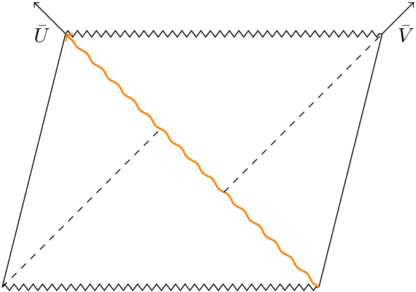
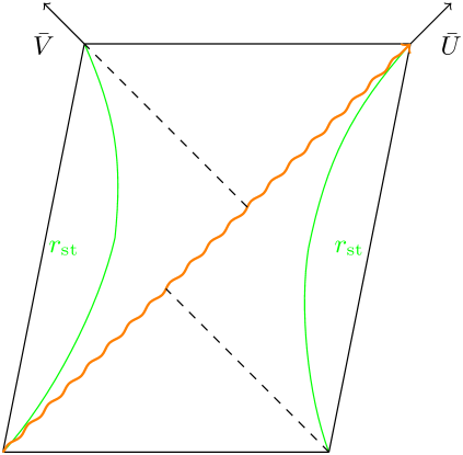
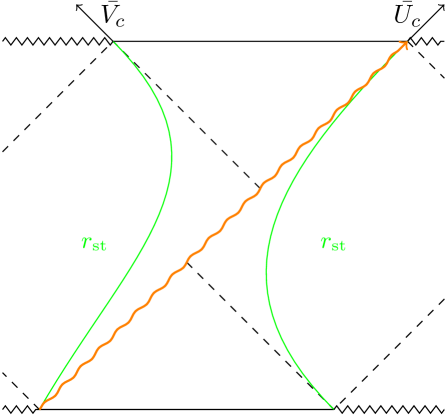
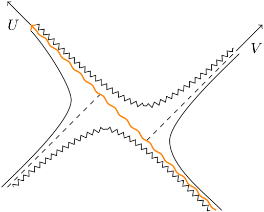
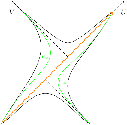
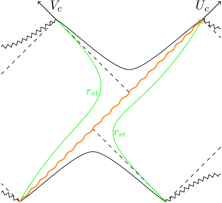
Figure 1: Shockwave geometry for an insertation along $U=0$ (orange wavy line) in: Schwarzchild-AdS_d+1≥4 (SAdS_d+1≥4) space (top, based on Shenker:2013pqa ), SdS₃ space (middle); and SdS_d+1≥4 space (bottom). Left column: Penrose diagrams in the $\bar{U}$, $\bar{V}$ coordinates defined in (12). Right column: Diagrams in Kruskal coordinates (10) with the modification $\alpha\rightarrow-\alpha$ in SAdS_d+1≥4 case. In the SdS geometries, the stretched horizon (in green) is shown at a fixed location $r=r_{\rm st}$. The cosmological and black hole horizons are shown with the dashed lines. In all cases, the $U$, $V$-axis are displayed with black arrows.

We are mainly interested in the metric under shockwave perturbations in the weak gravitational coupling regime to define the notions of energy below. We consider an SdS black hole with mass $M$ absorbs a shell of matter with mass $E\ll M$ along the surface

$$U=U_{0}=\mathrm{e}^{\frac{f^{\prime}(r_{\rm c})}{2}\left(r_{*}(r_{\mathcal{O}})-t_{0}\right)}\leavevmode\nobreak\ ,$$ (6)

with $t_{0}$ the static time shockwave insertion with respect to $r_{\mathcal{O}}$.

The SdS black hole after the shockwave has mass $M-E$ in (1) for matter obeying the NEC Baiguera:2023tpt ; Aguilar-Gutierrez:2023ymx . We glue the coordinates along a shell $U,\,V$ to the past of the shell with those to the future, denoted by $\tilde{U},\,\tilde{V}$. The resulting cosmological line element for SdS black holes Aguilar-Gutierrez:2023ymx ; Shenker:2013pqa :

$$\mathrm{d}s^{2}=-\frac{4\tilde{f}(r)}{\tilde{f}^{\prime}(r_{\rm c})}\mathrm{e}^{-\tilde{f}^{\prime}(\tilde{r}_{\rm c})\tilde{r}_{*}(r)}\mathrm{d}\tilde{U}\mathrm{d}\tilde{V}+r^{2}\mathrm{d}\Omega_{d-1}^{2}$$ (7)

where tilded quantities are given by the replacement of $M\rightarrow M-E$ in the untilded ones. In the inflating patch, the shift along the $V$ coordinate can be described by a shift in the coordinate

$$\tilde{V}=V-\alpha\leavevmode\nobreak\ .$$ (8)

The NEC also imposes that $\alpha\geq 0$ Aalsma:2021kle ; while $E\ll M$ guarantees we work in the $\alpha\ll 1$ limit. Importantly, this allows for the static patches in Fig. 1 to become causally connected, as it has been shown rigorously by Gao and Wald Gao:2000ga , in contrast to crunching geometries where the shift in $\alpha$ takes the opposite sign for matter satisfying the NEC.

We will express the shift parameter as

$$\alpha=2\mathrm{e}^{-\frac{f^{\prime}(r_{c})}{2}(t_{c}^{(*)}\pm t_{0})}\leavevmode\nobreak\ .$$ (9)

Here the $\pm$ sign depends on whether the shockwave is left or right moving, and the cosmological scrambling time $t_{c}^{(*)}$ will be defined through this relation.

We will take the shockwave close to the cosmological horizon and set $U_{0}=0$ in the following. (7) transforms into

$$\mathrm{d}s^{2}=-2A\quantity(U[V-\alpha\Theta(U)])\mathrm{d}U\mathrm{d}V+B\quantity(U[V-\alpha\Theta(U)])\mathrm{d}\Omega_{d-1}^{2}\leavevmode\nobreak\ ,$$ (10)

$$A\quantity(UV)=-\frac{2}{UV}\frac{f(r)}{f^{\prime}(r_{c})^{2}}\leavevmode\nobreak\ ,\quad B\quantity(UV)=r^{2}\leavevmode\nobreak\ .$$ (11)

Moreover, one can consider the change of coordinates

$$\bar{U}=\arctan U,\quad\bar{V}=\arctan V\leavevmode\nobreak\ ,$$ (12)

for the respective Penrose diagram (see Fig 1).

2.2 C=Anything: CMC slices

We are mainly interested in codimension-one observables within the class of the C=Anything proposal, introduced in Belin:2021bga ; Belin:2022xmt ,

$$\mathcal{C}^{\epsilon}\equiv\frac{1}{G_{N}}\int_{\Sigma_{\epsilon}}\mathrm{d}^{d}\sigma\,\sqrt{h}\leavevmode\nobreak\ F[g_{\mu\nu},\,\mathcal{R}_{\mu\nu\rho\sigma},\,\nabla_{\mu}]\leavevmode\nobreak\ ,$$ (13)

where $F[g_{\mu\nu},\,\mathcal{R}_{\mu\nu\rho\sigma},\,\nabla_{\mu}]$ is an arbitrary scalar functional of $d+1$-dimensional bulk curvature invariants, $\Sigma_{\epsilon}$ is a $d$-dimensional spatial slice labeled by $\epsilon$($=+,\,-$), which is anchored on the stretched horizon, $h$ is the determinant of the induced metric, $h_{\mu\nu}$, on $\Sigma_{\epsilon}$. We will let $F[\dots]$ be a general functional throughout the work. The reader is referred to footnote 8 to verify that these proposals display a switchback effect in AdS planar black holes in the time-reversal symmetrization in (46).

To define the region of evaluation, we employ a combination of codimension-one and codimension-zero volumes with different weights, given by

$$\mathcal{C}_{\rm CMC}=\frac{1}{G_{N}}\biggl{[} \alpha_{+}\int_{\Sigma_{+}}\mathrm{d}^{d}\sigma\,\sqrt{h}+\alpha_{-}\int_{\Sigma_{-}}\mathrm{d}^{d}\sigma\,\sqrt{h}+\alpha_{B}\int_{\mathcal{M}}\mathrm{d}^{d+1}x\sqrt{-g}\biggr{]}$$ (14)

where $\mathcal{M}$ is the bulk region; $\alpha_{\pm}$, $\alpha_{B}$ are constants; and $\Sigma_{+}$, $\Sigma_{-}$ are the future and past boundary slices in $\partial\mathcal{M}=\Sigma_{+}\cup\Sigma_{-}$, see Fig 2.

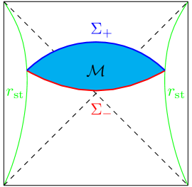
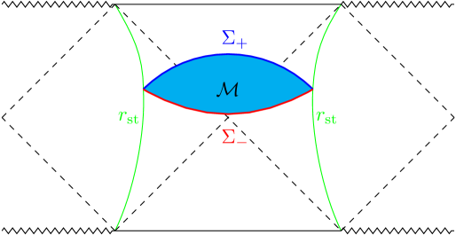
Figure 2: Implementation of the codimension-one CAny proposals with CMC slices, $\Sigma_{+}$ (blue) and $\Sigma_{-}$ (red) in the bulk region $\mathcal{M}$ (cyan), as evaluation regions in the unperturbed (S)dS space, following the same notation as in Fig. 1.

The extremization of $\mathcal{C}_{\rm CMC}$ reveals that $\Sigma_{\pm}$ are CMC slices, whose mean curvature is given by:

$$K_{\epsilon}\equiv\evaluated{K}_{\Sigma_{\epsilon}}=-\epsilon\frac{\alpha_{B}}{\alpha_{\epsilon}}\leavevmode\nobreak\ ,$$ (15)

where $K^{\mu\nu}=h^{\mu\alpha}\nabla_{\alpha}n^{\nu}$ is the extrinsic curvature, and we consider $n^{\mu}$ to be a future pointing normal vector for both $\Sigma_{\epsilon}$.

To simplify the evaluation of (13), we employ time-symmetric evolution on each of the static patches, so that we set $t_{L}=t_{R}$ in (1). Moreover, we introduce Eddington-Finkelstein coordinates in (1),

$$\mathrm{d}s^{2}=-f(r)\mathrm{d}v^{2}+2\mathrm{d}v\mathrm{d}r+r^{2}\mathrm{d}\Omega^{2}_{d-1}\leavevmode\nobreak\ ,$$ (16)

which are related to the Kruskal coordinates (4) by

$$U=\mathrm{e}^{-\frac{f^{\prime}(r_{c})}{2}u}\leavevmode\nobreak\ ,\quad V=-\mathrm{e}^{\frac{f^{\prime}(r_{c})}{2}v}\leavevmode\nobreak\ .$$ (17)

Evaluating (13, 14) with (1), one finds

$$\mathcal{C}^{\epsilon} =\frac{\Omega_{d-1}}{G_{N}}\int_{\Sigma_{\epsilon}}\mathrm{d}\sigma\,r^{d-1}\sqrt{-f(r)\dot{v}^{2}+2\dot{v}\dot{r}}\,a(r)\,,$$ (18)

$$\mathcal{C}_{\rm CMC} =\frac{\Omega_{d-1}}{G_{N}}\sum_{\epsilon}\alpha_{\epsilon}\int_{\Sigma_{\epsilon}}\mathrm{d}\sigma\,\mathcal{L}_{\epsilon}\leavevmode\nobreak\ ,$$ (19)

where $a(r)$ is a scalar functional corresponding to the evaluation of $F[g_{\mu\nu},\,\mathcal{R}_{\mu\nu\rho\sigma},\,\nabla_{\mu}]$; $\sigma$ is a general parametrization of the coordinates $v(\sigma)$, $r(\sigma)$ on the slice $\Sigma_{\epsilon}$; and

$$\mathcal{L}_{\epsilon}\equiv r^{d-1}\sqrt{-f(r)\dot{v}^{2}+2\dot{v}\dot{r}}-\epsilon\frac{K_{\epsilon}}{d}\dot{v}r^{d}\leavevmode\nobreak\ .$$ (20)

The details of the evaluation are shown in App. A. The late-time evolution of complexity results in:

$$\lim_{t\rightarrow\infty}\derivative{t}\mathcal{C}^{\epsilon}\simeq\frac{\Omega_{d-1}}{G_{N}}\sqrt{-f(r_{f})r_{f}^{2(d-1)}}\,a(r_{f})\leavevmode\nobreak\ \text{ with }r_{f}\equiv\lim_{t\rightarrow\infty}r_{t}\leavevmode\nobreak\ .$$ (21)

Here $r_{f}$ is a local maximum of the effective potential at late times:

$$\evaluated{\mathcal{U}}_{r_{f}}=0,\quad\evaluated{\partial_{{r}}\mathcal{U}}_{r_{f}}=0,\quad\evaluated{\partial^{2}_{{r}}\mathcal{U}}_{r_{f}}\leq 0\leavevmode\nobreak\ .$$ (22)

These conditions lead to the following relation

$$W(r_{f},\,K_{\epsilon})\equiv 4r_{f}f\left(r_{f}\right)\left((d-1)f^{\prime}\left(r_{f}\right)+K_{\epsilon}^{2}r_{f}\right)+4(d-1)^{2}f\left(r_{f}\right){}^{2}+r_{f}^{2}f^{\prime}\left(r_{f}\right){}^{2}=0\leavevmode\nobreak\ .$$ (23)

The roots $r_{f}$ of the function $W(r_{f},\,K_{\epsilon})$ can be found explicitly for pure dS and extremal SdS black hole limits, as originally derived in Aguilar-Gutierrez:2023zqm ,

$$\quantity({r}^{\rm(dS)}_{f})^{2} =\frac{{K_{\epsilon}}^{2}-2d(d-1)\pm|{K_{\epsilon}}|\sqrt{{K_{\epsilon}}^{2}-4(d-1)}}{2({K_{\epsilon}}^{2}-d^{2})}\leavevmode\nobreak\ ,\quad\absolutevalue{K_{\epsilon}}\geq 2\sqrt{d-1}\leavevmode\nobreak\ ;$$ (24)

$${r}^{\rm(N)}_{f} =\sqrt{\frac{d-2}{d}}\leavevmode\nobreak\ ,\quad\absolutevalue{K_{\epsilon}}\geq\sqrt{d}\leavevmode\nobreak\ .$$ (25)

Let us now show that for a generic SdS black hole spacetimes ($d\geq 3$), there will always be a real root to (23). One can evaluate $W(r_{f},\,K_{\epsilon})$ in (23) with the roots in (24, 25) while keeping the mass of the black hole arbitrary. We will denote $m\equiv\mu/\mu_{N}\in[0,\,1]$, such that we may express:

$$W\quantity({r}^{\rm(dS)}_{f},\,2\sqrt{d-1})=\frac{4m\left((d-2)^{d}d^{2}m-4(d-2)^{2}((d-1)d)^{d/2}\right)}{(d-2)^{4-d}(d-1)^{d-2}d^{d}}\leavevmode\nobreak\ ,$$ (26)

$$W\quantity({r}^{\rm(N)}_{f},\,K_{\epsilon})=\frac{4(1-m)\quantity(2K_{\epsilon}^{2}(d-2)+d^{2}(1-m))}{d^{2}}\leavevmode\nobreak\ .$$ (27)

Notice that (26) is clearly negative for all $d\geq 3$ and $m\in(0,\,1)$, while (27) is positive. Moreover, as we increase $\absolutevalue{K_{\epsilon}}>2\sqrt{d-1}$, $W\quantity({r}^{\rm(dS)}_{f},\,K_{\epsilon})$ becomes more negative in (23). Then, according to the intermediate value theorem, there will exist at least a real root ${r}_{f}\in\quantity[{r}^{\rm(dS)}_{f},\,{r}^{\rm(N)}_{f}]$ for general SdS_d+1 space.

On the other hand, since we have allowed $a(r)$ to be an arbitrary function in (21), we see that when $r_{f}\rightarrow\infty$ there would be arbitrary types of late-time growth for $C^{\epsilon}$ depending on the particular choice of $a(r)$. For instance, the case $a(r)=1$ leads to late-time exponential behavior when $r_{f}\rightarrow\infty$; meanwhile, having a different degree of divergence in (21) would lead to enhancement or decrease in the late-time growth. However, for this to be a valid CAny proposal, we require also a modification, as explained below.

When one evaluates the early time evolution in (21) $t\rightarrow-\infty$, there is a sign flip in $K_{\epsilon}\rightarrow-K_{\epsilon}$. As a result, the rate of growth of the CAny observables at early and late times does not coincide for a given CMC slice. The future or past growth would be given by (21), while the other generates hyperfast growth. Importantly for us, the switchback effect is not respected in this case, as on requires a cancellation between early and late-time contributions to the complexity growth. We will make this more explicit below.

3 The switchback effect

We will study the set of observables (13, 14) in the shockwave geometry (10). We begin performing a sequence of an even number of shockwaves, $n$, in the inflating patch (i.e. $r\in[r_{\mathcal{O}},\,\infty]$). Let us denote ${t}_{1}$, ${t}_{2}$, …, ${t}_{n}$ as the insertion static patch times with respect to the stretched horizon in alternating insertion order, i.e. ${t}_{2k+1}>{t}_{2k}$, and ${t}_{2k}<{t}_{2k-1}$, restricted to $\absolutevalue{{t}_{i+1}-{t}_{i}}\gg{t}_{*}$. Fig. 3 illustrates the multiple shockwave configuration in SdS space. The reader is referred to Shenker:2013pqa ; Stanford:2014jda for the asymptotic AdS black hole counterpart.

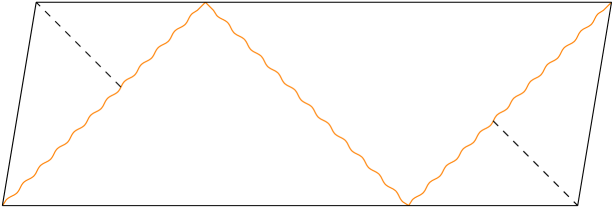
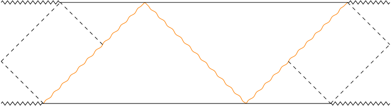
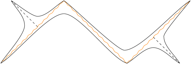
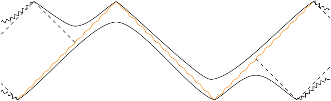
Figure 3: Multiple shockwave geometry in SdS₃ space (above) SdS_d+1≥4 space (below). Left column: (12) coordinates, and right column: (4) coordinates. The figure shows two forward-evolving and one backward-evolving pulse, producing the corresponding shift (9).

Accounting for the sign of the shift in the backreacted metric (10), the functional (13) has an additive property under these insertions in the strong shockwave limit Belin:2021bga ; Belin:2022xmt ,

$${\mathcal{C}}^{\epsilon}(t_{L},\,t_{R})= \mathcal{C}^{\epsilon}(t_{R},\,V_{1})+\mathcal{C}^{\epsilon}(V_{1}-\alpha_{1},\,U_{2})+\dots$$ (28)

$$+\mathcal{C}^{\epsilon}(U_{n-1}+\alpha_{n-1},\,V_{n})+\mathcal{C}^{\epsilon}(V_{n}-\alpha_{n},\,t_{L})$$

where all the contributions $\mathcal{C}^{\epsilon}(\cdot,\,\cdot)$ follow the same definition (13), but $\Sigma_{\epsilon}$ is anchored between endpoints that are located either on the left/right cosmological horizon, $r_{c}$, or on the stretched horizon $r_{\rm st}$. The different cases are illustrated in Fig. 4.

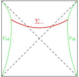
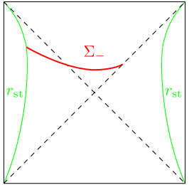
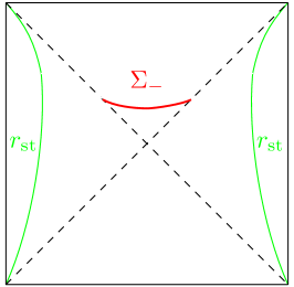
Figure 4: Different configurations of the extremal complexity surface $\Sigma_{\epsilon}$ appearing in (28) and illustrated for $\epsilon=-$ in SdS₃ space. Left: $\mathcal{C}^{-}(t_{L},\,t_{R})$, center: $\mathcal{C}^{-}(V_{R},\leavevmode\nobreak\ t_{L})$, and right: $\mathcal{C}^{-}(V_{R},\leavevmode\nobreak\ U_{L})$.

We can perform the evaluation of $\mathcal{C}^{\epsilon}$ by searching the locations $u_{R,\,L}$, $v_{R,\,L}$ where $\Sigma_{\epsilon}$ intersect with the left/right horizon $r_{c}$,

$$v_{R}-v_{t}=\int_{r_{c}}^{r_{t}}\mathrm{d}r\frac{\dot{v}}{\dot{r}}=\int_{r_{c}}^{r_{t}}\frac{\mathrm{d}r}{f(r)}\quantity(1-\frac{P_{v}^{\epsilon}+\frac{\epsilon K_{\epsilon}}{d}r^{d}}{\sqrt{-\mathcal{U}(P_{v}\epsilon,\,r)}})\leavevmode\nobreak\ ,$$ (29)

and $v_{t}=v_{R}(r_{t})$.

Next, we will use the boost symmetry in the static patch to set symmetric time evolution ($t_{L}=t_{R}=t/2$, which also implies $u_{L,\leavevmode\nobreak\ R}=v_{R,\leavevmode\nobreak\ L}$). The different contributions in (28) can be expressed with EF coordinates (16) as:

$$\mathcal{C}^{\epsilon}(t_{R},\,U_{L})=\mathcal{C}^{\epsilon}(V_{R},\,t_{L}) =-\frac{\Omega_{d-1}}{G_{N}}a(r_{t})\sqrt{-f(r_{t})r_{t}^{2(d-1)}}\quantity(\int_{r_{\rm st}}^{r_{t}}+\int_{r_{c}}^{r_{t}})\frac{\left(P_{v}^{\epsilon}+\frac{\epsilon K_{\epsilon}}{d}r^{d}\right)\mathrm{d}r}{f(r)\sqrt{-\mathcal{U}(P_{v}^{\epsilon},r)}}\leavevmode\nobreak\ ,$$ (30)

$$\mathcal{C}^{\epsilon}(V_{R},\,U_{L}) =-\frac{2\Omega_{d-1}}{G_{N}}a(r_{t})\sqrt{-f(r_{t})r_{t}^{2(d-1)}}\int_{r_{c}}^{r_{t}}\frac{\left(P_{v}^{\epsilon}+\frac{\epsilon K_{\epsilon}}{d}r^{d}\right)\mathrm{d}r}{f(r)\sqrt{-\mathcal{U}(P_{v}^{\epsilon},r)}}\leavevmode\nobreak\ .$$ (31)

As outlined in App. A (see (53)), we can express (18) as:

$${\mathcal{C}^{\epsilon}}(V_{R},\,U_{L})= -\frac{2\Omega_{d-1}}{G_{N}}a(r_{t})\sqrt{-f(r_{t})r_{t}^{2(d-1)}}\int_{r_{c}}^{r_{t}}\frac{\left(P_{v}^{\epsilon}+\frac{\epsilon K_{\epsilon}}{d}r^{d}\right)\mathrm{d}r}{f(r)\sqrt{-\mathcal{U}(P_{v}^{\epsilon},r)}}$$ (32)

$$+\frac{2\Omega_{d-1}}{G_{N}}\int_{r_{c}}^{r_{t}}\frac{a(r)f(r)\,r^{2(d-1)}+a(r_{t})\sqrt{-f(r_{t})r_{t}^{2(d-1)}}\left(P_{v}^{\epsilon}+\frac{\epsilon K_{\epsilon}}{d}r^{d}\right)}{f(r)\sqrt{-\mathcal{U}(P_{v}^{\epsilon},\,r)}}\leavevmode\nobreak\ .$$

Moreover, one may Taylor expand the effective potential (22) around the final slice, $r_{f}$, as

$$\lim_{r\rightarrow r_{f}}\mathcal{U}(P_{v}^{\epsilon},\,r)\simeq\frac{1}{2}(r-r_{f})^{2}\mathcal{U}^{\prime\prime}(P_{v}^{\epsilon},\,r)+\mathcal{O}(\absolutevalue{r-r_{f}}^{3})\leavevmode\nobreak\ .$$ (33)

We can then evaluate (29, 32) with (33) to find

$${\mathcal{C}^{\epsilon}}(V_{R},\,U_{L})=\frac{\Omega_{d-1}}{G_{N}}P_{\infty}^{\epsilon}v\leavevmode\nobreak\ ,\quad P_{\infty}^{\epsilon}=a(r_{f})\sqrt{-f(r_{f})r_{f}^{2(d-1)}}$$ (34)

where $r_{f}$ is determined with (23). The results above (34, 21) can be used to express the contributions in (28) in Kruskal coordinates (17) as:

$${\mathcal{C}^{\epsilon}}(t_{R},\leavevmode\nobreak\ V_{L}) =\frac{\Omega_{d-1}}{G_{N}}P_{\infty}^{\epsilon}\log{V_{L}\mathrm{e}^{t_{R}}}\leavevmode\nobreak\ ,$$ (35)

$${\mathcal{C}^{\epsilon}}(V_{R},\leavevmode\nobreak\ U_{L}) =\frac{\Omega_{d-1}}{G_{N}}P_{\infty}^{\epsilon}\log{U_{L}V_{R}}\leavevmode\nobreak\ ,$$ (36)

$${\mathcal{C}^{\epsilon}}(V_{R},\leavevmode\nobreak\ t_{L}) =\frac{\Omega_{d-1}}{G_{N}}P^{\epsilon}_{\infty}\log{\mathrm{e}^{t_{L}}V_{R}}\leavevmode\nobreak\ .$$ (37)

However, there is also an early time contribution in the shockwave geometry, given by the term

$${\mathcal{C}^{\epsilon}}(V_{L},\,U_{R})=\frac{\Omega_{d-1}}{G_{N}}P_{-\infty}^{\epsilon}\log{V_{L}U_{R}}\leavevmode\nobreak\ ,$$ (38)

where

$$P_{-\infty}^{\epsilon}=a(r_{I})\sqrt{-f(r_{I})r_{I}^{2(d-1)}}\leavevmode\nobreak\ ,\leavevmode\nobreak\ \text{ with }\leavevmode\nobreak\ r_{I}=\lim_{t\rightarrow-\infty}r_{t}\leavevmode\nobreak\ .$$ (39)

As mentioned above in Sec. 2.2, for $t\rightarrow-\infty$, there is a sign flip in $K_{\epsilon}\rightarrow-K_{\epsilon}$. In that case, $r_{I}$ is a solution to (22, 23) with the appropriate modification of $K_{\epsilon}$. However, as we also pointed out, the CMC slices that display late time growth in the far past/future display hyperfast growth in the future/past respectively. Instead, consider a protocol where we evaluate (18) over different CMC slices in the past and future, such that there are always solutions $r_{f}$ and $r_{I}$ with respect to the stretch horizon evolution. (28) then transforms into

$${\mathcal{C}^{\epsilon}}(t_{L},\,t_{R})\simeq\frac{\Omega_{d-1}}{G_{N}}\Bigl{[} P_{\infty}^{\epsilon}\log(V_{1}\mathrm{e}^{t_{R}})+P_{-\infty}^{\epsilon}\log(V_{1}-\alpha_{1})U_{2}+P_{\infty}^{\epsilon}\log(U_{2}+\alpha_{2})V_{3}+\dots$$ (40)

$$+P_{\infty}^{\epsilon}\log((V_{n}-\alpha_{n})\mathrm{e}^{t_{L}})\Bigr{]}\leavevmode\nobreak\ .$$

We can then extremize (40) with respect to an arbitrary interception point ($V_{i}$, $U_{i}$) in the multiple shockwave geometry,

$$\derivative{{\mathcal{C}^{\epsilon}}(t_{L},\,t_{R})}{V_{i}}=0\leavevmode\nobreak\ ,\quad\derivative{{\mathcal{C}^{\epsilon}}(t_{L},\,t_{R})}{U_{i}}=0\leavevmode\nobreak\ ,$$ (41)

which allows us to locate

$$V_{i}^{\epsilon}=\frac{P_{\infty}^{\epsilon}\alpha_{i}}{P_{\infty}^{\epsilon}+P_{-\infty}^{\epsilon}}\leavevmode\nobreak\ ,\quad U_{i}^{\epsilon}=-\frac{P_{-\infty}^{\epsilon}\alpha_{i}}{P_{\infty}^{\epsilon}+P_{-\infty}^{\epsilon}}\leavevmode\nobreak\ .$$ (42)

Replacing the interception points into (40) generates:

$${\mathcal{C}^{\epsilon}}(t_{L},\,t_{R})\simeq\frac{\Omega_{d-1}}{G_{N}}\quantity(P_{\infty}^{\epsilon}(t_{R}+t_{L})+(P_{\infty}^{\epsilon}+P_{-\infty}^{\epsilon})\quantity(\sum_{k=1}^{n}t_{k}-nt^{(c)}_{*}))\leavevmode\nobreak\ ,$$ (43)

up to constant terms in terms of $P_{+\infty}^{\epsilon}$, $P_{-\infty}^{\epsilon}$.

Importantly, it was noticed in Aguilar-Gutierrez:2023zqm that the CAny proposals with a generic functional $F[\dots]$ in (19) for an AdS planar black hole background only satisfy the switchback effect when the rate of growth in the past and future are the same. This means that for (19) to obey the definition of holographic complexity in Belin:2021bga ; Belin:2022xmt , we require

$$P^{\epsilon}_{+\infty}=P^{\epsilon}_{-\infty}\leavevmode\nobreak\ .$$ (44)

In that case, the evaluation of (43) reduces to

$$\mathcal{C}^{\epsilon}(t_{L},\,t_{R})\propto\absolutevalue{t_{R}+t_{1}}+\absolutevalue{t_{2}-t_{1}}+\dots+\absolutevalue{t_{n}-t_{L}}-2nt^{(c)}_{*}\leavevmode\nobreak\ ,$$ (45)

where the term $-2nt^{(c)}_{*}$ appears due to cancellation in the complexity growth due to early and late time perturbations.

Notice that a possible way to satisfy (44) in SdS space can be obtained by setting $K_{-}=-K_{+}$ and selecting a complexity proposal $\mathcal{C}$ as

$$\mathcal{C}=\min_{t}\quantity(\mathcal{C}^{+}(t),\,\mathcal{C}^{-}(t))\leavevmode\nobreak\ .$$ (46)

See Fig. 5 for an illustration of the evolution of the CMC slices in the shockwave geometry.

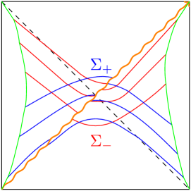
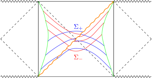
Figure 5: Representative CMC slices anchored to the stretched horizon (green) in a single shockwave geometry in SdS space. We employ the discontinuous Kruskal coordinates $\tilde{U}$, $\tilde{V}$ in (7) in the Penrose diagram to facilitate the representation of the CMC slices.

We close the section with a few remarks. First, the result (45) reproduces the same type of behavior as the switchback effect for AdS planar black holes, at least for the CAny proposals with early and late-time linear growth in SdS space. Second, as we mentioned in Sec. 2.2 there are fine-tuned situations where $\mathcal{C}^{\epsilon}$ can have any type of early and late-time growth behavior for SdS₃. It might be interesting to study the modifications in the switchback in those cases. Lastly, the switchback effect has also been recovered in a different and more explicit analysis for particular asymptotically dS backgrounds Anegawa:2023dad ; Baiguera:2023tpt , hinting at the possibility that this is a rather universal phenomenon in shockwave geometries.

4 Discussion and outlook

In summary, we studied the appearance of the switchback effect in asymptotically dS spacetimes by studying the late (and early time) evolution of the codimension-one CAny observables under shockwave insertions. We picked a set of observables that are evaluated in CMC slices of different curvature in the past and future boundaries. We proved that under a weakly gravitating regime, the CAny observables show a reduction in the complexity growth due to cancellations of the energy perturbations. We also explicitly verified one of the predictions in Aguilar-Gutierrez:2023zqm , namely that a time-reversal symmetric protocol would be necessary for the switchback effect to occur. Moreover, our findings show a great similarity with respect to the behavior of CAny proposals for AdS black holes under the switchback effect. However, we reiterate that the CAny observables in our study do not necessarily represent holographic complexity in asymptotically dS space. To have a clear notion of holographic complexity, we might require a quantum circuit interpretation for the observables, which would also require a reliable quantum circuit model for dS space. Some toy models allowing much progress in this direction have been studied in Bao:2017iye ; Bao:2017qmt ; Niermann:2021wco ; Cao:2023gkw .

We comment on some interesting future directions. Our work focused on the alternating shockwave insertion on the inflating patch of the SdS spacetime. However, we can also extend the analysis when the SdS spacetime has multiple patches, to enquire about the black hole interior as well. These types of geometries have been used as toy models for multiverses in Aguilar-Gutierrez:2021bns . One of the striking features previously found was that the information available to the past light cone of an observer in one of the multiverses would encode the information of the other universes, in the semiclassical regime. It would be very interesting to see whether the notions of general codimension-zero CAny observables may also encode such information. We might be able to learn if some of these observables might have an interpretation from the point of view of quantum cosmology. It might be also fruitful to study how the introduction of perturbations in the geometry affects the coarse-graining of information found in Aguilar-Gutierrez:2021bns .

An important aspect in the search for the holographic description of dS space would be obtaining a dual interpretation of the observables that we studied in this work. It would be interesting to analyze quantum circuit observables that display similar behaviors to the ones studied within our work to study whether the effect of perturbations on the stretched horizon might also have the interpretation of an epidemic type of growth given the insertion of operators. Moreover, it would be interesting to see what type of signals can be found in a UV complete description of the stretched horizon, motivated by the DSSYK model Susskind:2021esx ; Blommaert:2023opb .

Applications to of CAny to dS space braneworld models were recently carried out in Aguilar-Gutierrez:2023tic to gain more information about dS holography. In these models Randall:1999ee ; Randall:1999vf , one includes an end-of-the-world brane, whose tension determines the cosmological constant in the effective gravitational theory on the brane. It would be interesting to incorporate the switchback effect to characterize perturbations in a double holographic setting, with a clearer field theory dual. This effective theory might be further modified by adding intrinsic gravity theories on the brane, leading to a more intricate holographic complexity evolution Hernandez:2020nem ; ACHKKS ; AL . Moreover, the fluctuations associated with the brane location lead to an effective description as dS JT gravity on one of the branes Aguilar-Gutierrez:2023tic . It would be interesting to study the switchback effect of this effective theory.

On the other hand, as we found in Fig. 2, the CAny observables generically reach a terminal turning $r_{f}$ (as well as a time-reversal version) determined by the choice of the CMC slices through (23). This implies that the CAny proposals in the article do not prove the whole cosmological patch of SdS spacetime. However, we would expect that any notion of static patch holography should also encode the degrees of freedom of the inflating region, similar to investigations in asymptotically AdS space Jorstad:2023kmq . Nevertheless, one can probe more of the geometry outside the cosmological horizon using the alternating shockwave geometry. It seems that adding perturbations in the stretched horizon reveals more information, even when its explicit localization is irrelevant.

Finally, much progress in the dS holography has been made possible through the study of interpolating geometries in two-dimensional dilaton-gravity theories Anninos:2017hhn ; Anninos:2018svg ; Anninos:2020cwo ; Anninos:2022hqo ; Aguilar-Gutierrez:2023odp ; AESV . While the CV proposal has been extensively studied in Chapman:2021eyy for certain interpolating geometries; new members in this set have recently appeared Anninos:2022hqo , and the CAny proposals have not been treated yet. This might allow for a clearer interpretation of the properties studied in this work in the context of dS₂ space, appearing from near extremal limits near horizon limits of black hole geometries Maldacena:2019cbz ; Castro:2022cuo .

Appendix A Details on the CAny evaluation

For the choice

$$\sqrt{-f(r)\dot{v}^{2}+2\dot{v}\dot{r}}=r^{d-1}\leavevmode\nobreak\ ,$$ (47)

the Euler-Lagrange equations corresponding to (19) can be expressed as

$$\dot{r}^{2}+\mathcal{U}(P_{v}^{\epsilon},\,r)=0\leavevmode\nobreak\ ,$$ (48)

where

$$P_{v}^{\epsilon} \equiv\partialderivative{\mathcal{L}_{\epsilon}}{\dot{v}}=\dot{r}-\dot{v}\,f(r)-\epsilon\frac{K_{\epsilon}}{d}\,r^{d}\leavevmode\nobreak\ ;$$ (49)

$$\mathcal{U}(P_{v}^{\epsilon},\,r) \equiv-f(r)r^{2(d-1)}-\left(P_{v}^{\epsilon}+\epsilon\frac{K_{\epsilon}}{d}r^{d}\right)^{2}\leavevmode\nobreak\ .$$ (50)

Then, we can express (18) as

$$\mathcal{C}^{\epsilon}=\frac{2\Omega_{d-1}}{G_{N}}\int_{r_{\rm st}}^{r_{t}}\frac{r^{2(d-1)}a(r)}{\sqrt{-\mathcal{U}(P_{v}^{\epsilon},\,r)}}\mathrm{d}r\leavevmode\nobreak\ .$$ (51)

In a similar way, the parameter $t$ can be expressed as

$$t =\int_{\Sigma_{\epsilon}}\mathrm{d}r\frac{\dot{t}}{\dot{r}}=\int_{\Sigma_{\epsilon}}\mathrm{d}r\frac{\dot{v}-\dot{r}/{f(r)}}{\sqrt{-\mathcal{U}(P_{v}^{\epsilon},\,r)}}$$ (52)

$$=-2\int_{r_{\rm st}}^{r_{t}}\frac{\mathrm{d}r}{f(r)\,\sqrt{-\mathcal{U}(P_{v}^{\epsilon},r)}}\left(P_{v}^{\epsilon}+\frac{\epsilon K_{\epsilon}}{d}r^{d}\right)\leavevmode\nobreak\ .$$

We proceed to evaluate (51) with (52) carefully. Since $U(P_{v}^{\epsilon},\,r_{t})=0$ by definition, we need to take care of the denominator in (51, 52) at each of the turning points. We do so by adding a subtracting a term:

$${\mathcal{C}^{\epsilon}}= -\frac{2\Omega_{d-1}}{G_{N}}a(r_{t})\sqrt{-f(r_{t})r_{t}^{2(d-1)}}\int_{r_{\rm st}}^{r_{t}}\frac{\left(P_{v}^{\epsilon}+\frac{\epsilon K_{\epsilon}}{d}r^{d}\right)\mathrm{d}r}{f(r)\sqrt{-\mathcal{U}(P_{v}^{\epsilon},r)}}$$ (53)

$$+\frac{2\Omega_{d-1}}{G_{N}}\int_{r_{\rm st}}^{r_{t}}\frac{a(r)f(r)\,r^{2(d-1)}+a(r_{t})\sqrt{-f(r_{t})r_{t}^{2(d-1)}}\left(P_{v}^{\epsilon}+\frac{\epsilon K_{\epsilon}}{d}r^{d}\right)}{f(r)\sqrt{-\mathcal{U}(P_{v}^{\epsilon},\,r)}}\leavevmode\nobreak\ .$$

Then, we can identify the relationship between time in (52) and complexity in (53)

$${\mathcal{C}^{\epsilon}}= \frac{\Omega_{d-1}}{G_{N}}a(r_{t})\sqrt{-f(r_{t})r_{t}^{2(d-1)}}t$$ (54)

$$+\frac{2\Omega_{d-1}}{G_{N}}\int_{r_{\rm st}}^{r_{t}}\frac{a(r)f(r)\,r^{2(d-1)}+a(r_{t})\sqrt{-f(r_{t})r_{t}^{2(d-1)}}\left(P_{v}^{\epsilon}+\frac{\epsilon K_{\epsilon}}{d}r^{d}\right)}{f(r)\sqrt{-\mathcal{U}(P_{v}^{\epsilon},\,r)}}\leavevmode\nobreak\ .$$

We can then straightforwardly take the time derivative,

$${\derivative{\mathcal{C}^{\epsilon}}{t}}= \frac{\Omega_{d-1}}{G_{N}}a(r_{t})\sqrt{-f(r_{t})r_{t}^{2(d-1)}}$$ (55)

$$+\frac{2\Omega_{d-1}}{G_{N}}\derivative{P_{v}^{\epsilon}}{t}\int_{r_{\rm st}}^{r_{t}}\mathrm{d}r\frac{r^{2(d-1)}\left(a(r_{t})\sqrt{-f(r_{t})r_{t}^{2(d-1)}}-a(r)\quantity(P_{v}^{\epsilon}+\frac{\epsilon K_{\epsilon}}{d}r^{d})\right)}{\quantity(-\mathcal{U}(P_{v}^{\epsilon},\,r))^{3/2}}\leavevmode\nobreak\ .$$

Thus, in the $t\rightarrow\infty$ regime we then recover (21). Moreover, the $\derivative{P_{v}^{\epsilon}}{t}$ term vanishes (21) provided that the effective potential reaches a maximum Jorstad:2023kmq , shown in (22).

References

- (1) L. Susskind, Entanglement is not enough, Fortsch. Phys. 64 (2016) 49 [1411.0690].
- (2) L. Susskind, Computational Complexity and Black Hole Horizons, Fortsch. Phys. 64 (2016) 24 [1403.5695].
- (3) D. Stanford and L. Susskind, Complexity and Shock Wave Geometries, Phys. Rev. D 90 (2014) 126007 [1406.2678].
- (4) B. Czech, Einstein Equations from Varying Complexity, Phys. Rev. Lett. 120 (2018) 031601 [1706.00965].
- (5) P. Caputa and J.M. Magan, Quantum Computation as Gravity, Phys. Rev. Lett. 122 (2019) 231302 [1807.04422].
- (6) L. Susskind, Complexity and Newton’s Laws, Front. in Phys. 8 (2020) 262 [1904.12819].
- (7) J.F. Pedraza, A. Russo, A. Svesko and Z. Weller-Davies, Lorentzian Threads as Gatelines and Holographic Complexity, Phys. Rev. Lett. 127 (2021) 271602 [2105.12735].
- (8) J.F. Pedraza, A. Russo, A. Svesko and Z. Weller-Davies, Sewing spacetime with Lorentzian threads: complexity and the emergence of time in quantum gravity, JHEP 02 (2022) 093 [2106.12585].
- (9) J.F. Pedraza, A. Russo, A. Svesko and Z. Weller-Davies, Computing spacetime, Int. J. Mod. Phys. D 31 (2022) 2242010 [2205.05705].
- (10) S. Chapman and G. Policastro, Quantum computational complexity from quantum information to black holes and back, Eur. Phys. J. C 82 (2022) 128 [2110.14672].
- (11) A.R. Brown, D.A. Roberts, L. Susskind, B. Swingle and Y. Zhao, Holographic Complexity Equals Bulk Action?, Phys. Rev. Lett. 116 (2016) 191301 [1509.07876].
- (12) A.R. Brown, D.A. Roberts, L. Susskind, B. Swingle and Y. Zhao, Complexity, action, and black holes, Phys. Rev. D 93 (2016) 086006 [1512.04993].
- (13) J. Couch, W. Fischler and P.H. Nguyen, Noether charge, black hole volume, and complexity, JHEP 03 (2017) 119 [1610.02038].
- (14) A. Belin, R.C. Myers, S.-M. Ruan, G. Sárosi and A.J. Speranza, Does Complexity Equal Anything?, Phys. Rev. Lett. 128 (2022) 081602 [2111.02429].
- (15) A. Belin, R.C. Myers, S.-M. Ruan, G. Sárosi and A.J. Speranza, Complexity equals anything II, JHEP 01 (2023) 154 [2210.09647].
- (16) D.A. Galante, Modave lectures on de Sitter space & holography, PoS Modave2022 (2023) 003 [2306.10141].
- (17) L. Susskind, Entanglement and Chaos in De Sitter Space Holography: An SYK Example, JHAP 1 (2021) 1 [2109.14104].
- (18) E. Shaghoulian and L. Susskind, Entanglement in De Sitter space, JHEP 08 (2022) 198 [2201.03603].
- (19) L. Susskind, Scrambling in Double-Scaled SYK and De Sitter Space, 2205.00315.
- (20) H.W. Lin, The bulk Hilbert space of double scaled SYK, JHEP 11 (2022) 060 [2208.07032].
- (21) H. Lin and L. Susskind, Infinite Temperature’s Not So Hot, 2206.01083.
- (22) B. Bhattacharjee, P. Nandy and T. Pathak, Krylov complexity in large- and double-scaled SYK model, 2210.02474.
- (23) A.A. Rahman, dS JT Gravity and Double-Scaled SYK, 2209.09997.
- (24) L. Susskind, De Sitter Space has no Chords. Almost Everything is Confined, 2303.00792.
- (25) L. Susskind, A Paradox and its Resolution Illustrate Principles of de Sitter Holography, 2304.00589.
- (26) V. Franken, H. Partouche, F. Rondeau and N. Toumbas, Bridging the static patches: de Sitter holography and entanglement, JHEP 08 (2023) 074 [2305.12861].
- (27) H.W. Lin and D. Stanford, A symmetry algebra in double-scaled SYK, 2307.15725.
- (28) E. Jørstad, R.C. Myers and S.-M. Ruan, Holographic complexity in dSd+1, JHEP 05 (2022) 119 [2202.10684].
- (29) R. Auzzi, G. Nardelli, G.P. Ungureanu and N. Zenoni, Volume complexity of dS bubbles, Phys. Rev. D 108 (2023) 026006 [2302.03584].
- (30) T. Anegawa and N. Iizuka, Shock waves and delay of hyperfast growth in de Sitter complexity, JHEP 08 (2023) 115 [2304.14620].
- (31) S. Baiguera, R. Berman, S. Chapman and R.C. Myers, The cosmological switchback effect, JHEP 07 (2023) 162 [2304.15008].
- (32) T. Anegawa, N. Iizuka, S.K. Sake and N. Zenoni, Is action complexity better for de Sitter space in Jackiw-Teitelboim gravity?, JHEP 06 (2023) 213 [2303.05025].
- (33) S.E. Aguilar-Gutierrez, M.P. Heller and S. Van der Schueren, Complexity = Anything Can Grow Forever in de Sitter, 2305.11280.
- (34) S.E. Aguilar-Gutierrez, A.K. Patra and J.F. Pedraza, Entangled universes in dS wedge holography, 2308.05666.
- (35) S.H. Shenker and D. Stanford, Black holes and the butterfly effect, JHEP 03 (2014) 067 [1306.0622].
- (36) S.E. Aguilar-Gutierrez, R. Espíndola and E.K. Morvan-Benhaim, A teleportation protocol in Schwarzschild-de Sitter space, 2308.13516.
- (37) S.E. Aguilar-Gutierrez, A. Chatwin-Davies, T. Hertog, N. Pinzani-Fokeeva and B. Robinson, Islands in Multiverse Models, JHEP 11 (2021) 212 [2108.01278].
- (38) S. Gao and R.M. Wald, Theorems on gravitational time delay and related issues, Class. Quant. Grav. 17 (2000) 4999 [gr-qc/0007021].
- (39) L. Aalsma, A. Cole, E. Morvan, J.P. van der Schaar and G. Shiu, Shocks and information exchange in de Sitter space, JHEP 10 (2021) 104 [2105.12737].
- (40) S.V. der Schueren, Master thesis, gent university, 2023.
- (41) M.A. Nielsen, A geometric approach to quantum circuit lower bounds, Quantum Info. Comput. 6 (2006) 213–262 [quant-ph/0502070].
- (42) M.A. Nielsen, M.R. Dowling, M. Gu and A.C. Doherty, Quantum computation as geometry, Science 311 (2006) 1133.
- (43) M.R. Dowling and M.A. Nielsen, The geometry of quantum computation, arXiv preprint quant-ph/0701004 (2006) .
- (44) N. Bao, C. Cao, S.M. Carroll and L. McAllister, Quantum Circuit Cosmology: The Expansion of the Universe Since the First Qubit, 1702.06959.
- (45) N. Bao, C. Cao, S.M. Carroll and A. Chatwin-Davies, De Sitter Space as a Tensor Network: Cosmic No-Hair, Complementarity, and Complexity, Phys. Rev. D 96 (2017) 123536 [1709.03513].
- (46) L. Niermann and T.J. Osborne, Holographic networks for (1+1)-dimensional de Sitter space-time, Phys. Rev. D 105 (2022) 125009 [2102.09223].
- (47) C. Cao, W. Chemissany, A. Jahn and Z. Zimborás, Overlapping qubits from non-isometric maps and de Sitter tensor networks, 2304.02673.
- (48) A. Blommaert, T.G. Mertens and S. Yao, Dynamical actions and q-representation theory for double-scaled SYK, 2306.00941.
- (49) L. Randall and R. Sundrum, A Large mass hierarchy from a small extra dimension, Phys. Rev. Lett. 83 (1999) 3370 [hep-ph/9905221].
- (50) L. Randall and R. Sundrum, An Alternative to compactification, Phys. Rev. Lett. 83 (1999) 4690 [hep-th/9906064].
- (51) J. Hernandez, R.C. Myers and S.-M. Ruan, Quantum extremal islands made easy. Part III. Complexity on the brane, JHEP 02 (2021) 173 [2010.16398].
- (52) S.E. Aguilar-Gutierrez, B. Craps, J. Hernandez, M. Khramtsov, M. Knysh and A. Shukla, Time dependence of holographic complexity for planar ads black holes with an end of the world brane, to appear.
- (53) S.E. Aguilar-Gutierrez and F. Landgren, to appear.
- (54) E. Jørstad, R.C. Myers and S.-M. Ruan, Complexity=anything: singularity probes, JHEP 07 (2023) 223 [2304.05453].
- (55) D. Anninos and D.M. Hofman, Infrared Realization of dS2 in AdS2, Class. Quant. Grav. 35 (2018) 085003 [1703.04622].
- (56) D. Anninos, D.A. Galante and D.M. Hofman, De Sitter horizons & holographic liquids, JHEP 07 (2019) 038 [1811.08153].
- (57) D. Anninos and D.A. Galante, Constructing AdS2 flow geometries, JHEP 02 (2021) 045 [2011.01944].
- (58) D. Anninos and E. Harris, Interpolating geometries and the stretched dS2 horizon, JHEP 11 (2022) 166 [2209.06144].
- (59) S.E. Aguilar-Gutierrez, E. Bahiru and R. Espíndola, The centaur-algebra of observables, 2307.04233.
- (60) S.E. Aguilar-Gutierrez, R. Espíndola, A. Svesko and M.R. Visser, deformations from ads2 to ds2, to appear.
- (61) S. Chapman, D.A. Galante and E.D. Kramer, Holographic complexity and de Sitter space, JHEP 02 (2022) 198 [2110.05522].
- (62) J. Maldacena, G.J. Turiaci and Z. Yang, Two dimensional Nearly de Sitter gravity, JHEP 01 (2021) 139 [1904.01911].
- (63) A. Castro, F. Mariani and C. Toldo, Near-extremal limits of de Sitter black holes, JHEP 07 (2023) 131 [2212.14356].