Cosmic Evolution Early Release Science Survey (CEERS): Multi-classing Galactic Dwarf Stars in the deep JWST/NIRCam

Abstract

Low mass (sub)stellar objects represent the low end of the initial mass function, the transition to free-floating planets and a prominent interloper population in the search for high-redshift galaxies. Without proper motions or spectroscopy, can one identify these objects photometrically? JWST/NIRCam has several advantages over HST/WFC3 NIR: more filters, a greater wavelength range, and greater spatial resolution. Here, we present a catalogue of (sub)stellar dwarfs identified in the Cosmic Evolution Early Release Science Survey (CEERS). We identify 518 stellar objects down to mF200W 28 using half-light radius, a full three magnitudes deeper than typical HST/WFC3 images. A kNN nearest neighbour algorithm identifies and types these sources, using four HST/WFC3 and four NIRCam filters, trained on SpeX spectra of nearby brown dwarfs. The kNN with four neighbors classifies well within two subtypes: e.g M2$\pm$2 or T4$\pm$2, achieving $\sim$95% precision and recall. More granular typing results in worse metrics. In CEERS, we find 9 M8$\pm$2, 2 L6$\pm$2, 1 T4$\pm$2, and 15 T8$\pm$2. We compare the observed long wavelength NIRCam colours —not used in the kNN— to those expected for brown dwarf atmospheric models. The NIRCam F356W-F444W and F410M-F444W colours are redder by a magnitude for the type assigned by the kNN, hinting at a wider variety of atmospheres for these objects. We find a 300-350pc scale-height for M6$\pm$2 dwarfs plus a second structural component and a 150-200pc scale-height for T6$\pm$2 type dwarfs, consistent with literature values.

1 Introduction

With the successful start of operations of the NASA/ESA/CSA’s James Webb Space Telescope (JWST) a new window has opened up on the lowest mass stars of our Milky Way. These near-infrared stellar objects are interlopers in the new, deep extra-galactic observations, but low-mass (sub)stellar members of the Milky Way also encode information on the shape and history of our Galaxy. Here, we report the numbers of such low-mass (sub)stellar objects found in the Cosmic Evolution Early Release Science Survey (CEERS, Finkelstein et al., 2022a) collaborations first NIRCam observations (Bagley et al., 2022).

Counting stars to infer the morphology and scales of the Milky Way is a classic experiment in Astronomy. This was the original motivation behind mapping the night sky, begun initially with photographic plates, moving to wide-field CCDs, and now space-based imaging with missions such as the Hubble and Webb Space Telescopes.

However, counting stars is also an approach that can easily fall into conceptual problems and incomplete information (e.g., Herschel 1785; Kapteyn, 1922). The disk of the Milky Way was eventually measured and mapped using Giant stars with ever increasing precision (Gilmore & Reid, 1983; Gilmore, 1984; Siegel et al., 2002). The statistics are now such that individual stellar kinematic populations can be tracked (e.g. Hsu et al., 2021) and a link between the scales of the disk and metallicity is evident (e.g. Bovy et al., 2012).

Near-infrared mapping of the sky has revealed dwarf galaxy populations in the local solar neighbourhood (Reid et al., 2001; Cruz et al., 2004). Thanks to the WISE satellite (Wright et al., 2010), a near-complete census of the nearest 20 parsecs around our Sun, the numbers of these brown dwarfs are now known, adding a spectral class in the process (Reid et al., 2008; Kirkpatrick et al., 2021).

These lower-mass stars have gained attention as a nuisance population in the search with the Hubble Space Telescope and now James Webb Space Telescope for high-redshift ($z>>6$) galaxies blackas both populations overlap in color space (Caballero et al., 2008; Wilkins et al., 2014; Finkelstein, 2015). This provides a completely independent scientific motivation to characterize blackthe number of ultracool dwarfs in the Milky Way.

Deep Hubble observations have constrained the size of the Milky Way disk thanks to the unambiguous identifications of stars as point sources as even high redshift galaxies are resolved and enough colours or grism spectra exist for type identification. Brown dwarfs have been identified in the Hubble Deep Field (Pirzkal et al., 2005), GOODS/CANDELS fields (Stanway et al., 2008; Pirzkal et al., 2009) and individual parallel fields (Ryan et al., 2005, 2011; Holwerda et al., 2014b; van Vledder et al., 2016). But with low statistics and only a few lines of sight out of our Milky Way, these studies remain uncertain on the scale-height, especially as a function of brown dwarf (sub)type.

Ryan et al. (2017) introduces a new concept to model the scale-height for different sub-types of brown dwarfs: it implies that as brown dwarf’s atmospheres cool black(i.e. these objects age and thus become a later type), their population scatters and kinematically heats up, resulting in a greater Galactic scale-height. Depending on the star-formation history of the Milky Way, this cooling/aging effect with kinematic heating of the population as a whole, should be clear in the brown dwarf type-scale-height relation. Ryan et al. (2022) refined the above model and included the kinematic tracers showing direct evidence for the vertical mixing of this populationAganze et al. (2022a, b). Additional prior constraints can come from the local IMF (Kirkpatrick et al., 2021), local 3D T-dwarf kinematics (Hsu et al., 2021), and the previous determined scale-heights (Aganze et al., 2022a, b) from blackthe WFC3 Infrared Spectroscopic Parallel Survey WISPS grism observations. blackThese Hubble Space Telescope searches for brown dwarfs are limited to $m_{J}=24$AB for pure-parallel photometry and grism observations.

The challenge is therefore to type M/L/T/Y dwarf objects sufficiently accurately to map their distances photometrically. The broad filters typically employed on JWST/NIRCam deep observations such as CEERS (Finkelstein et al., 2022a) and PEARLS (Windhorst et al., 2023) programs may hold enough information to do so (Holwerda et al., 2018). blackThe CEERS NIRCam observations were in a large part designed to identify sources for follow-up with the other JWST instruments to characterize their nature (see Bisigello et al., 2023; Carnall et al., 2023; Coogan et al., 2023; Costantin et al., 2023; Arrabal Haro et al., 2023b, a; Gómez-Guijarro et al., 2023; Long et al., 2023; Magnelli et al., 2023; Shen et al., 2023a; Vega-Ferrero et al., 2023; Kocevski et al., 2023a; Larson et al., 2023). Our aim here is to evaluate how suitable such JWST/NIRCam observations are for Galactic science, specifically low-mass (sub)stellar objects.

Here, we explore the use of the colour space of the early CEERS NIRCam observations to identify (sub)stellar objects in these fields. We classify them using the templates of nearby examples using k-nearest neighbours. And finally we constrain the scale-height of the Milky Way using the identified (sub)stellar populations in the CEERS field, and compare these with existing estimates.

2 CEERS

The Cosmic Evolution Early Release Science Survey (CEERS, PI: S. Finkelstein; Finkelstein et al., 2017) is a JWST early release science (ERS) project to explore the early Universe and the early evolution of galaxies using a variety of instrument modes, shortly after telescope commissioning (Rigby et al., 2023b, a).

CEERS has covered $\sim$90 sq. arcmin of the EGS field with JWST (Menzel et al., 2023; McElwain et al., 2023; Gardner et al., 2023) imaging (and a portion with spectroscopy) using NIRCam (Rieke et al., 2023) described in Bagley et al. (2023), MIRI (Wright et al., 2023) described in blackYang et al. (in preparation), and NIRSpec (Jakobsen et al., 2022; Böker et al., 2023) described in blackArrabal Haro et al. (in preparation). CEERS demonstrates, tests, and validates efficient extragalactic surveys with coordinated, overlapping parallel observations in a field supported by a rich set of HST/CANDELS multi-wavelength imaging (Grogin et al., 2011; Koekemoer et al., 2011). blackThe CEERS NIRCam data were obtained in two epochs, in June and December 2022.

The CEERS science goals include the identification of high-redshift galaxies through NIRCam colours (Akins et al., 2023; Finkelstein et al., 2022b), confirming candidate high-redshift sources with NIRSpec or ground-based follow-up (e.g. Fujimoto et al., 2022, 2023), and probe the physical conditions in these early galaxies using emission line diagnostics and mid-infrared emission (Arrabal Haro et al., 2023b, a; Jung et al., 2022, 2023; Tang et al., 2023; Zavala et al., 2023). The NIRCam filters are sensitive to rest-frame optical emission and thus ideal to probe the evolution of structure starting at a much earlier epoch than ever before (Guo et al., 2023; Long et al., 2023; Huertas-Company et al., 2023; Magnelli et al., 2023; Shen et al., 2023b; Vega-Ferrero et al., 2023). These two science topics, the identification for follow-up of high-redshift targets and the structure of earlier epoch galaxies were the main drivers of the observational design. The early science methodology and results are presented in a series of Key Papers (Finkelstein et al., 2023; Kocevski et al., 2023b; Kartaltepe et al., 2023; Papovich et al., 2023; Pérez-González et al., 2023; Yang et al., 2023). Key for these science aims is the NIRCam imaging for discovery and characterization of sources in this field. However, these CEERS JWST/NIRCam observations have been designed from the start to explore and characterize extragalactic topics and no special consideration was given for Galactic science.

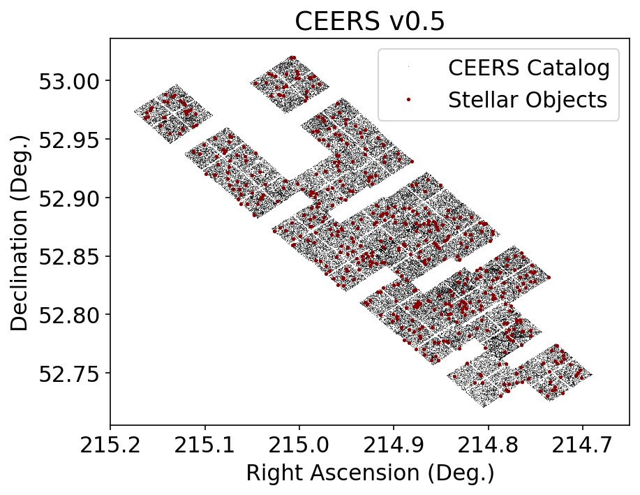
Figure 1: Small black dots denote all objects in the CEERS photometric catalog used for this work. The red dots denote the positions of stellar objects identified in Figure 2.

3 Data

The JWST/NIRCam images used are the pixel-aligned mosaics described in Bagley et al. (2023), v0.6 on the CEERS website. Empirical PSFs were created by stacking stars for the entire mosaic in the case of HST and NIRCam.

We make use of the internal CEERS photometry catalog. This will be discussed in Finkelstein et al. (in prep.), but the methodology is summarized here. The PSF of F606W, F814W, F115W, F150W and F200W is matched to that of F277W (see Table LABEL:t:observations). For bands with larger PSFs, the redder NIRCam filters, F356W and F444W, and all other HST/WFC3 filters, they calculated correction factors by convolving the shorter wavelength images to the larger PSF of the F444W, and measuring the flux ratio in the native image to that in the convolved image. By applying this correction factor the fluxes measured in the images with larger PSFs, this corrects for the missing flux under the assumption that the morphology does not change significantly. This is especially useful for small high-redshift sources or faint stellar photometry as it is used here. The photometry using Source Extractor (v2.25.0 Bertin & Arnouts, 1996; Holwerda, 2005) is described in Finkelstein et al (in prep).

The fits catalog contains photometry in units of nJy. We made use of the fiducial flux and flux error columns, which were corrected to total, and with flux errors calculated empirically from the images. Fluxes were converted to AB magnitudes using a conversion of $\rm m_{AB}(FILTER)=-2.5\times log_{10}(FLUX\_FILTER)+31.4$. The F277W+F356W image was the detection image with the other filters run in dual-image mode to obtain photometry (see Finkelstein et al., 2022a, Finkelstein in preparation for details). The half-light radius from Source Extractor for the F200W filter image is included in this catalogue. The position of all the sources in the catalogue is shown in Figure 1.

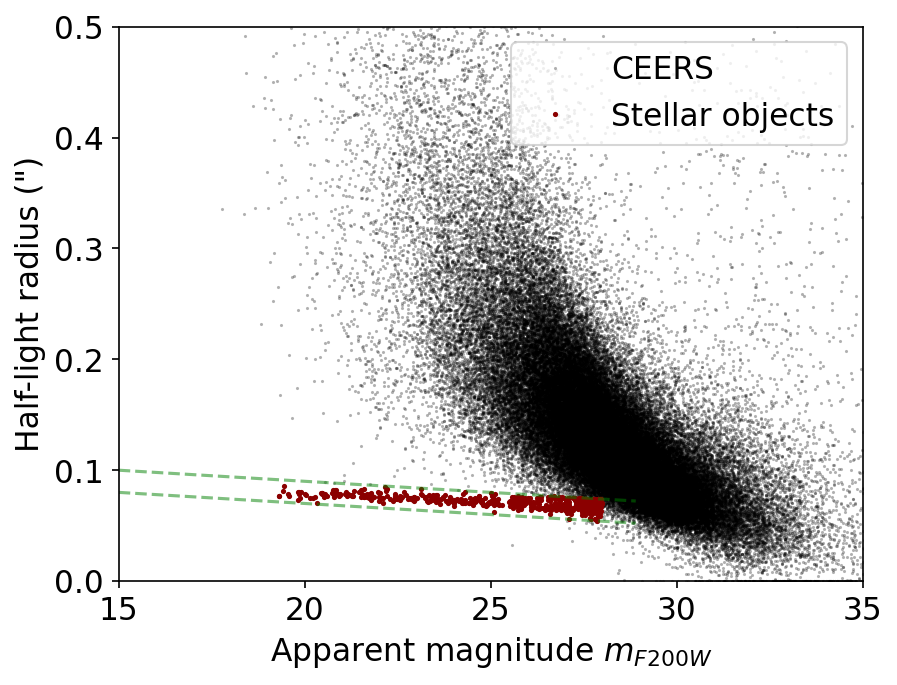
Figure 2: The apparent magnitude of objects in the CEERS photometric catalogue in the F200W detection filter (AB magnitude) and the effective radius computed by Source Extractor in the same filter. The green dashed lines delineate the locus of unresolved sources. We identify the red objects as unresolved stellar candidates.

3.1 Stellar Catalog

We use the effective radius measured in the F200W image of the two-image Source Extractor run described above to identify unresolved objects in the stellar locus. Figure 2 shows the effective radius as a function of the F200W AB magnitude. The green dashed lines show the limits of the stellar locus, similar to the approach in Ryan et al. (2011) and Holwerda et al. (2014b). The unresolved stars’ half-light radius is less than 0$\aas@@fstack{\prime\prime}$1 and declines slightly with fainter objects. blackThis is a known effect in HST imaging because the growth curve from which Source Extractor derives the half-light radius loses the lower surface brightness pixels which make a larger fraction for the flux for fainter sources. The red marks in Figure 2 are the stellar candidates marked in Figure 1 as well. The utility of the half-light radius measured by Source Extractor translates well from HST to JWST with a slightly different dependence between the half-light radius and magnitude. We empirically determine that this stellar identification works well to m${}_{AB}\sim 28$ for the CEERS field.

We use AB magnitudes derived to determine colours for the three feature spaces, JWST/NIRCam, HST+JWST combined, or either ranked by filter wavelength or colours based on only HST and JWST filter pairs.

Figure 3 shows the NIRCam colours space with the SpeX Prism Library Analysis Toolkit (SPLAT) template stellar colours overplot of increasing type (Burgasser & Splat Development Team, 2017; Holwerda et al., 2018). A majority of the stellar objects have colours similar to brown dwarf templates.

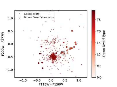
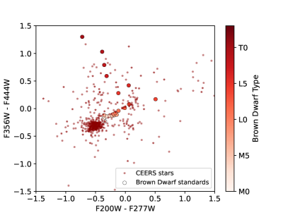
Figure 3: The F115W-F150 and F200W-F277W, F200W-F277W and F356W-F444W colour-colour space for the stellar objects identified in Figure 2 with the brown dwarf standard stars overplot as tracks in increasing type. With the intrinsic variation in colour with brown dwarf type, this shows it is plausible a majority of the stellar sources are possibly brown dwarf type objects. No F410M filter information is available for the standard brown dwarfs.

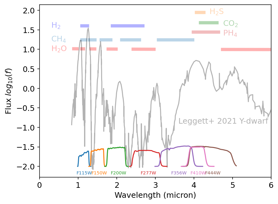
Figure 4: An example of a Y-dwarf from Leggett et al. (2021) with some of the absorbing molecule species marked and the CEERS NIRCam filters used annotated at the bottom. The JWST/NIRCam blue filters (F115W, F150W, F200W and F277W) are sensitive to the molecular absorption features that define the classes. The longer wavelength filters (F356W, F410M, and F444W) are more sensitive to overall temperature and different molecular absorption features.

4 Classifying M-l-T-Y type dwarfs with NIRCam colours

A problem in identifying M-L-T-Y dwarf stars from just photometry is that, while there are some clear absorption features in their spectra in the 0.5-2 micron range, these easily become a somewhat degenerate space when observed with wide filters of current and near-future near-infrared imaging space observatories (Holwerda et al., 2018). blackFigure 4 shows an example of a Y-dwarf spectrum from Leggett et al. (2021) with the CEERS NIRCam filter curves to illustrate. Depending on the atmospheric composition of the brown dwarf, one can expect very different NIRCam colours.

The challenge is now to classify as well as possible with just NIRCam broad colours. Previous work (Ryan et al., 2011; Holwerda et al., 2014b) solved this with colour-colour spaces defined in HST filters. The issue is that these are hard cuts in colour space and the problem of broad classification is not as clear-cut as that.

Here, we use the JWST/NIRCam colour predictions based on SPLAT spectral library from Holwerda et al. (2018) to classify unresolved sources in CEERS. To do so, we tried k-means Nearest neighbour (kNN), a support vector machine (SVM) and a random forest (RF, an average of decision trees) on the bluest colours. Because the SPLAT spectra only extend to 2.5$\mu m$, the longest NIRCam wavelengths cannot be included for the training of the ML algorithms but we can compare the resulting type predictions to the standard stars for each type, for which there is analogue WISE satellite W1-W2 colour available.

blackBecause the colour space of brown dwarfs represents a space with steep gradients and a mixture of physical parameters that drive the observed NIR spectra, we prefer this approach over fitting templates to each SED with assuming the lowest $\chi^{2}$ is the optimal fit. By using SPLAT observed spectra rather than model templates, the kNN fit allows for observed but still unexplained variance in each type.

4.1 Training Sample

The full JWST/NIRCam colour sample available based on SPLAT spectroscopy (Burgasser & Splat Development Team, 2017) is described in Holwerda et al. (2018). Briefly, there is JWST/NIRCam photometry estimates for the black30 standard stars which define the spectral type and for all the SPLAT spectra which capture the intermediate types and variance within spectral types. We use the latter as a training set. The photometry from Holwerda et al. (2018) is in Vega magnitudes and we convert to AB magnitudes first. There is NIR colours in both HST/WFC3 and JWST/NIRCam filters. We use three blackcolour feature spaces, a NIRCam-only, a NIRCam and HST one with colours separated by instrument, and a third where colours use filters in wavelength order, mixing HST and JWST filters.

For the labels one can employ index-type or standard_type from the SPLAT catalog (Burgasser & Splat Development Team, 2017), the blacklatter a classification by the spectral index and the former the class to which standard star they resemble most. The indextype has fewer stars classified as intermediate than the standard_type does. We adopt the standard_type throughout. We assign a numerical type as follows: M-types are 0-0.9, L-types 1.0-1.9, T-types 2.0-2.9 and Y-types 3 and above. Later, when applying these labels to the kNN multi-classing, we multiply these by 10 because the kNN can only handle integer classes. Late M- and early L-types blackare much more represented in the SPLAT training set compared to the later types because their relative luminosity. But all types and subtypes are present in the training set with reasonable sampling (Figure 5).

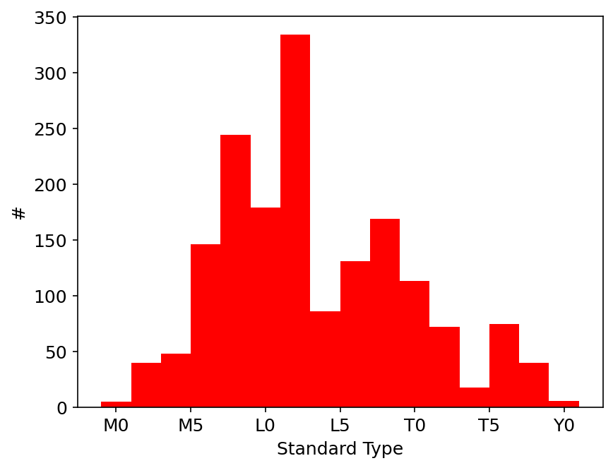
Figure 5: The distribution of standard types for the SPLAT training set. The training set is dominated by late M- and early L-dwarfs.

Ryan et al. (2011) and Holwerda et al. (2014b) used the near-infrared colour-colour space to broadly type the M-L-T dwarfs in parallel HST/WFC3 fields. Figure 6 shows the original HST/WFC3 colour-colour space used for broad photometric typing of these objects. Broad classes are still mixed in this colour space and subtyping blackusing hard cuts in colour-colour space is not possible.

Figure 7 shows a NIRCam equivalent of a colour-colour plot of the SPLAT catalog. A similar separation of objects could conceivably be used. Rather than picking a particular colour-colour combination for broad classification and hoping to sub-class these objects with the remaining information, we opt to subclass directly, varying the blackspectral subtype resolving power ($\Delta T$). As said above, we use three feature spaces: the bluer NIRCam colours, and two iterations of the CEERS HST+JWST complete photometry, one using only instrument specific colours (inst), i.e. only combining HST filters into a colour, and one with the colours arranged by wavelength (wav). For example, in the latter, we combine HST’s F160W and NIRCam’s F150W into a single colour.

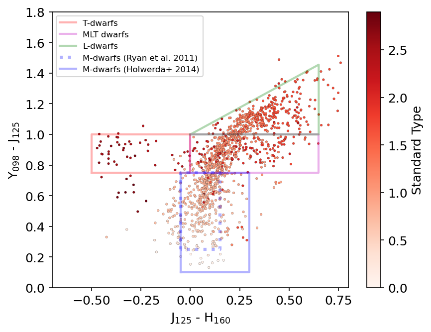
Figure 6: The distribution of HST/WFC3 colours for the standard types for the training set. The colour-colour selections from Ryan et al. (2011) and Holwerda et al. (2014b) for M-, L-, and T-dwarfs are indicated with coloured boxes. This illustrates the issue with hard cuts: in a two-dimensional space like this, there is still ample mixing of types. A photometric classifier based on proximity in this space is expected to perform better than these initial colour-colour cuts.

Figures 7, 8 and 9 show the parameter space and the classification into broad types as the colour-coding. Colour-colour space has already proven itself to work well on broad type (e.g. M, L, T or Y?) but now we will attempt to refine the classification down to subclasses.

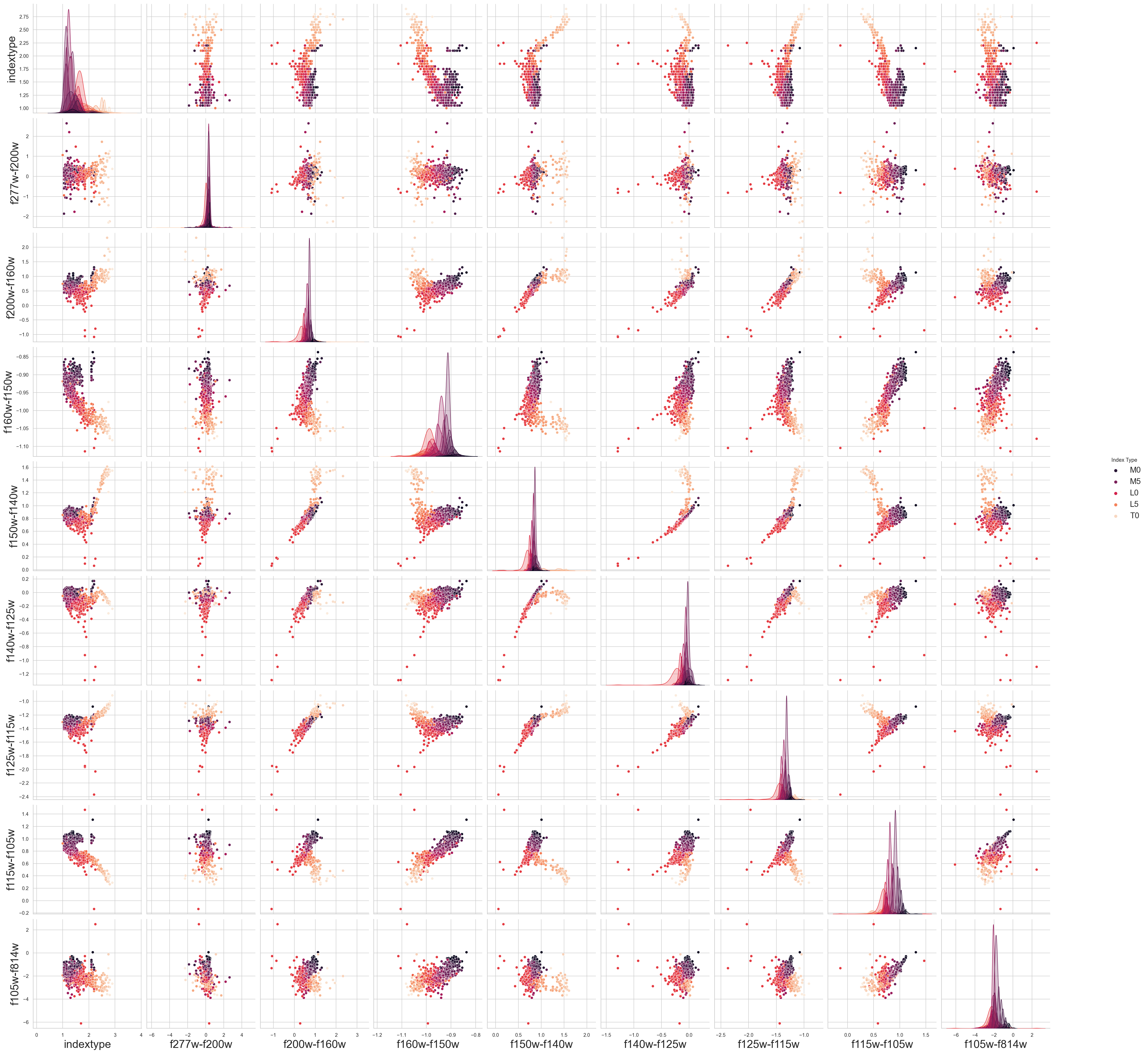
Figure 7: The full feature space of the photometric catalog generated from SPLAT spectra of nearby brown dwarfs for the JWST/NIRCam filters in CEERS. Some parts of the colour-colour space are well-suited to broadly classify these objects but the space is degenerate, an ideal scenario to maximize return with a machine learning approach.

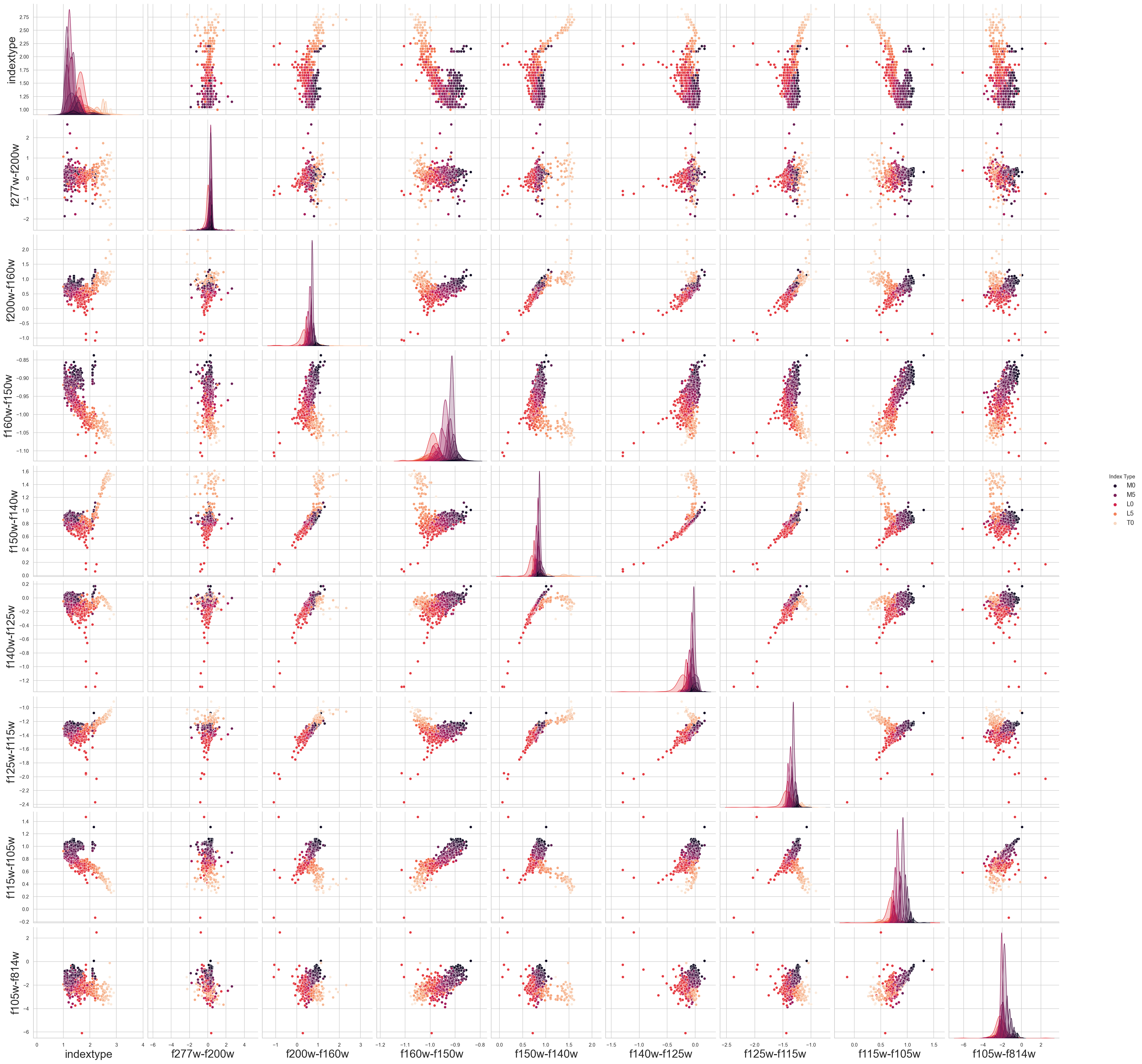
Figure 8: The full feature space of the photometric catalog generated from SPLAT spectra of nearby brown dwarfs for the HST/WFC3 filters in CEERS. Some parts of the colour-colour space are well-suited to broadly classify these objects but the space is degenerate, an ideal scenario to maximize return with a machine learning approach.

We start to classify based on 1271 SPLAT (Burgasser & Splat Development Team, 2017; Holwerda et al., 2018) spectra from which photometry can be derived in Holwerda et al. (2018) with spectral classifications (standard type). There are 40 classes in this training set.

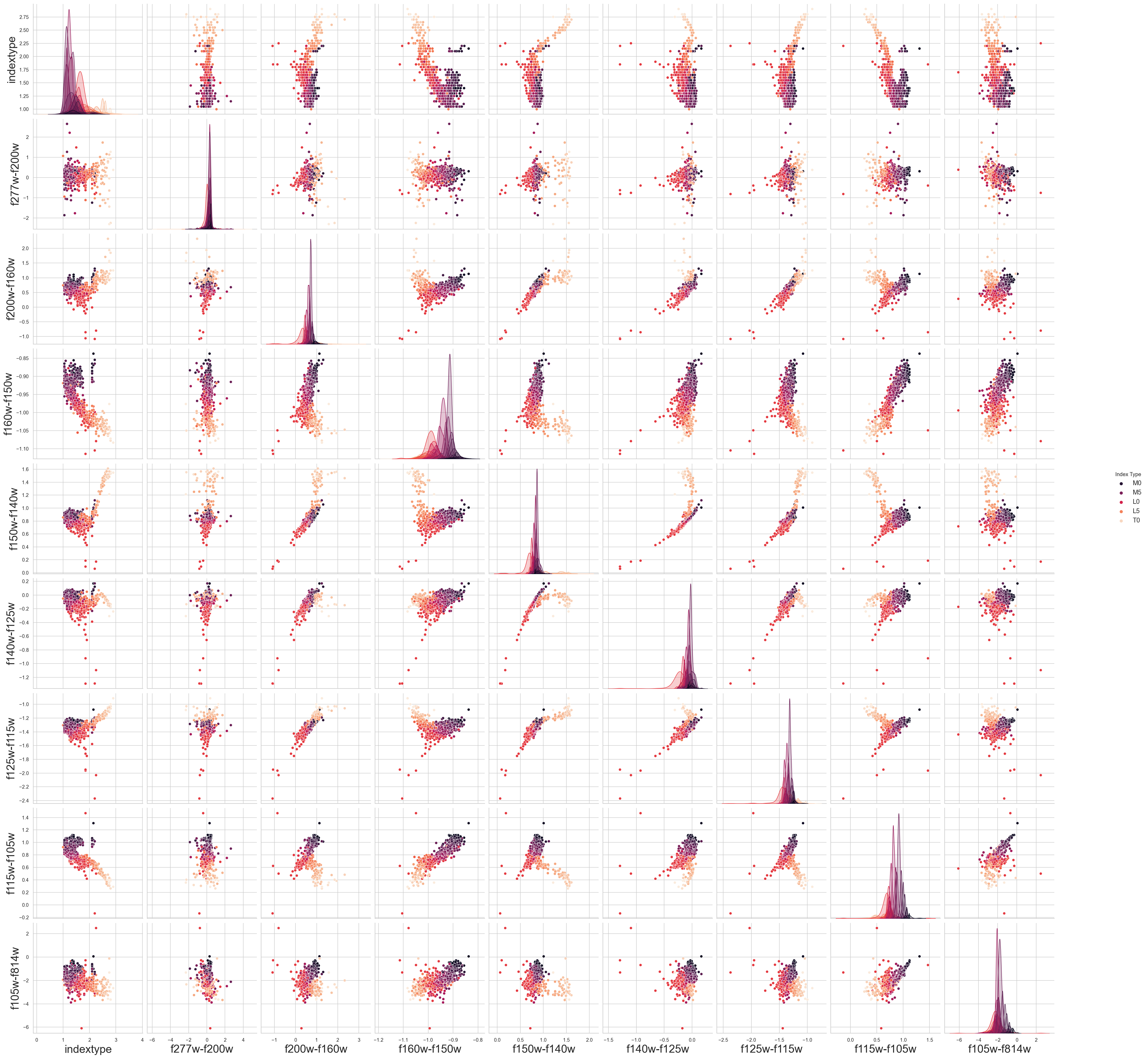
Figure 9: The full JWST+HST feature space of the photometric catalog generated from SPLAT spectra of nearby brown dwarfs for the HST/WFC3 and JWST/NIRCam filters in the CEERS catalog, sorted by wavelength. This extensive colour feature space may well be suited to classify sources in deep HST+JWST data but mixing instruments for the colours may be susceptible to systematics.

4.2 kNN Classifications

K-Nearest Neighbour classifies objects using the N nearest neighbours in the feature space. Historically, kNN classifies in to two classes (0 or 1). MultiClass classification can be defined as the classifying instances into one of three or more classes. Multiclassing is possible with the sklearn implementation of kNN and this is what we employ here. blackkNN classification has successfully been used on brown dwarf photometry in Marengo & Sanchez (2009). Splitting the SPLAT sample into the typical 80/20 per cent split between training and test set, we classify into the 40 classes of standard type. We initially use the HST+JWST(wav) feature space where colours are computed going from longest to shortest wavelength of the filter, regardless of instrument used.

We want to know a few different classification specific questions: (1) How many neighbours are optimal for classification in this feature space? (2) To what degree of accuracy can one classify within 0.1 of a subtype, 0.2, 0.5 or just the full type? (3) How well does it still perform if only JWST or HST information is used?

4.3 Number of Neighbours

Figure 10 shows the dependence of the kNN performance trained on the full HST+JWST(wav) feature space as a function of the number of neighbours used, the key hyperparameter for kNN classifiers. blackMetrics are calculated based on the number of true and false positives and negatives (TP, FP, TN and FN) in case of two classes. Our metrics are accuracy (TP+TN / TP+TN+FP+FN), precision (TP/TP+FP), recall (TP/TP+FN), and F1 (2$\times$ precision $\times$ recall / precision+recall). A good classifier strikes a balance between accuracy (fraction of accurate classifications), the accuracy of positive identification (precision), and the completeness of the identified sample (recall) or a metric of the balance of the previous two (F1). The optimal performance in terms of accuracy occurs between n=3 and n=7. Precision and F1 peak at n=4. We use n=4 for the remainder of our applications of kNN on these data-sets as the optimal number of neighbours to determine subtype with kNN. blackThis is comprable to k=3 adopted for Spitzer colour classification adopted by Marengo & Sanchez (2009).

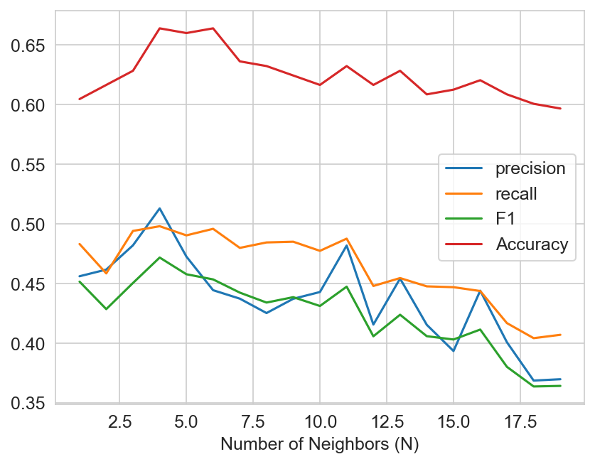
Figure 10: The precision, recall, blackF1, and accuracyblack, each expressed as a dimensionless fraction, as a function of number of neighbours (n) of the test set of the kNN classifier on the SPLAT photometry using the HST+JWST(wav) feature space.

4.4 Performance and type accuracy

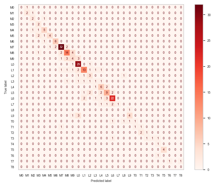
Figure 11: The confusion matrix of the kNN classification into individual subtypes of M, L, T-dwarfs using the HST+JWST(wav) feature space shown in Figure 9. The overall metrics can be found in Table 1 for a type resolution of $\Delta T=0.1$

Figure 11 shows the confusion matrix over all 40 types of standard type classes in the training set $\Delta T=0.1$, the highest type accuracy possible. Accuracy was 66% and the other metrics are in Table 1. The same feature space using the indextype as the label performed notably worse. This level of performance is not useful in classification but the confusion matrix in Figure 11 is encouraging in that it may improve with a somewhat coarser type resolution.

Instance	Accuracy	Precision	Recall	F1
kNN $\Delta T$	(%)	(%)	(%)	(%)
0.1	0.60	0.46	0.49	0.46
0.2	0.77	0.62	0.62	0.61
0.3	0.77	0.78	0.79	0.78
0.4	0.83	0.83	0.82	0.82
0.5	0.83	0.70	0.70	0.70
0.6	0.83	0.68	0.68	0.68
0.7	0.86	0.82	0.82	0.82
0.8	0.91	0.69	0.71	0.69
0.9	0.89	0.88	0.91	0.89
1.0	0.89	0.92	0.93	0.92

Table 1: The metrics for the different binning in type for the kNN algorithm. An optimal resolution is $\Delta T=0.5$ for this colour-space.

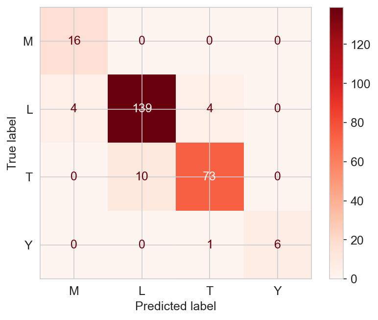
Figure 12: The broad black($\Delta T=1$) kNN classification confusion matrix

Secondly, we explore if just broad class (M/L/T or 0/1/2) classifications can be done with this feature space. Accuracy dramatically improves to 85% with equally good precision and recall scores. These values were even higher for indextype, probably because it does not contain M-type which is somewhat featureless in the NIR blackat the spectral resolution of these filters. Figure 12 shows the confusion matrix for standard type class for just the broad class for classification. Broad types one can do very well with these four broad JWST/NIRCam filters. There is a slight tendency of kNN algorithm to class brown dwarfs as later type (below the diagonal).

Figure 13: The kNN classification confusion matrix on the HST+JWST(wav) feature space with a much lower type resolution of $\Delta T=0.5$

Our question is now how much better the classification can do than broad class? First, we classify within half a class, within $\Delta T=0.5$, where the integer is the broad M, L or T class and then we shall explore 0.4 and 0.2 of a class. Because kNN algorithm does not allow for fractional classes, we multiply the class by 10 (e.g. L1 thus becomes 11 and we divide by 10 afterwards).

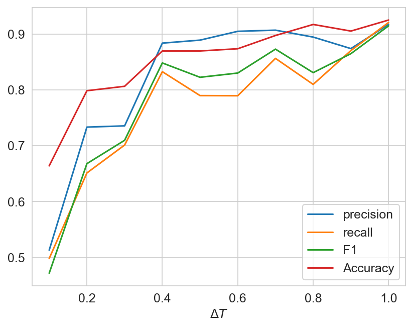
Figure 14: The metrics of the kNN classificationblack, each expressed as a dimensionless fraction, as a function of the type resolution ($\Delta T$) for the full HST+JWST/NIRCam. All metrics climb steadily with coarser type resolution. If one wants to classify within a type ($\Delta T=0.5$), the metrics are $\sim 85$%. Notably, $\Delta T=0.3$ would perform almost equally well.

blackFigures 12 and 13 show the confusion matrices for the different resolutions in spectral type for the test set. Figure 14 shows the metrics of the test set for kNNs trained with different spectral type resolution and these metrics for each kNN run are listed in Table 1.

Figure 15: The kNN classification confusion matrix on the HST+JWST(wav) feature space with the optimal type resolution of $\Delta T=0.4$. This is the kNN classifier used on the CEERS photometry

black Figure 15 shows the optimal type resolution of $\Delta T=4$ with k=4. This is the optimum we can achieve with the mix of filters available in CEERS. We note that HST or JWST filter combinations alone also perform optimally with this spectral type resolution but with lower overall metrics (Figure 16).

We varied the number of neighbours for each classification scheme (e.g. blackn=2 to n=20) but this made no real difference in the metrics. blackJust under half a type black($\Delta T=0.4$) clearly is the optimal resolution for the HST three-colour feature space to classify in. This is a substantial improvement the hard colour cuts into broad type by Ryan et al. (2011) and Holwerda et al. (2014b) but falls just short of grism spectroscopy classification which can discriminate between subtypes (Aganze et al., 2022a, b).

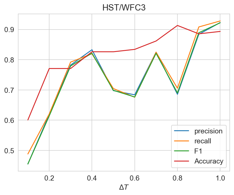
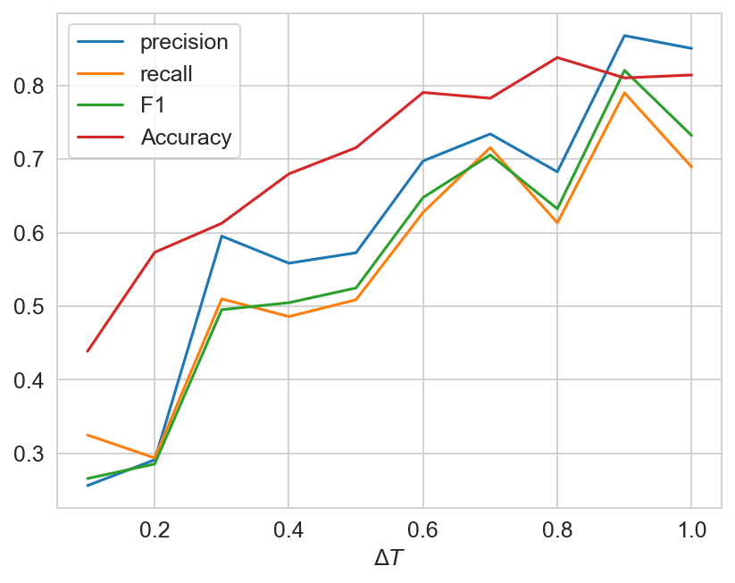
Figure 16: The metrics of the kNN classificationblack, each expressed as a dimensionless fraction, as a function of the type resolution ($\Delta T$) for the HST-only filter colour-space (left) and the JWST-only filter colour-space (right). For HST, all metrics climb steadily with coarser type resolution. If one wants to classify within a type ($\Delta T=0.5$), the metrics are $\sim 85$%. Notably, $\Delta T=0.4$ would perform almost equally well. For JWST-only, the blue NIRCam filers perform poorer than in combination with HST (Fig. 14) or HST-only (left) until almost full type resolution $\Delta T\sim 1$

Figure 16 shows the type resolution of HST-only and JWST/NIRCam-only colour feature spaces. Surprisingly, the HST filter combination performs almost as well as HST+JWST/NIRCam in classification accuracy with type resolution (Figure 14). In effect, it appears that kNN classification can be almost as accurate if the HST NIR imaging is sufficiently deep enough to identify the relevant stars. This will be an inherently smaller volume than JWST/NIRCam can reach.

stars	M4	M8	L2	L6	T0	T4	T8
518	491	9	0	2	0	1	15

Table 2: The numbers of stellar objects identified in the NIRCam fields and the the respective classifications by the KNN. Both M4 and T8 may include types that are hotter and more massive or colder respectively (e.g. K-start in the M0 or Y3-dwarfs in the T8 category).

5 Results

We will now examine the use of the kNN classification on the NIRCam observations of CEERS described in §3.

5.1 Application to CEERS

We now apply the kNN classification on the CEERS photometry of unresolved sources identified in Figure 2. Figure 1 shows the distribution of unresolved sources in the ten CEERS fields. We identified a total of 518 stars with a classification ($P_{kNN}>0.5$) with the majority of probabilities at 0.8 (Table 2). These classifications are based on the colours using the F115W, F150W, F200W, and F277W filters. We can now verify these kNN type predictions with the red NIRCam colours.

5.2 NIRCam Red colours

Figure 17 shows the kNN type versus the F444W-F356W and F444W-F410M colours. These colours are not included in the SPLAT derived filters as these wavelengths are outside the SpeX spectrograph bandwidth. However, WISE W1-W2 colours are available for the standard stars for each type from Pecaut & Mamajek (2013) and these are close stand-ins for the F444W-F356W colour. These colours can be computed for the models of Saumon et al. (2012) and Morley et al. (2012) L/T/Y atmospheric models as well. The standard stars agree well with these atmospheric models, blackspecifically those of Saumon et al. (2012). We note that there is almost a magnitude of variance in colour in the models of Morley et al. (2012), reflecting a wider range of parameters.

The CEERS kNN identified late brown dwarf types ($T>2.5$, T5 dwarf or later) appear to be bluer in the NIRCam reddest filters, the ones not used in the kNN classification. These are some 7 high-confidence blackbrown dwarfs ($P(T)>80$%) that do not line up in the redward colour space. blackThe discrepancy is as much as a magnitude in F444W-F356W colour. The remaining late-M and late-T types are much more consistent with the NIRCam long filters.

Figure 4 gives a hint to the discrepancy between the classification based on the short wavelength filters and the colours observed in the long NIRCam filters. The F410M and F444W both cover a wavelength range where a Sulfur and a Phosphorus molecule is influencing absorption (Leggett et al., 2021). If these are T/Y dwarfs with relatively more of such compounds, perhaps it could skew the reddest NIRCam colours blacktowards redder values?

blackThe Saumon et al. (2012) and Morley et al. (2012) models are for Solar metallicity brown dwarfs only. This explains why they align with the standards for brown dwarfs and hints at lower metallicity as a possible explanation for the red colours of these late-type brown dwarfs. Future infrared spectroscopy of these could confirm this.

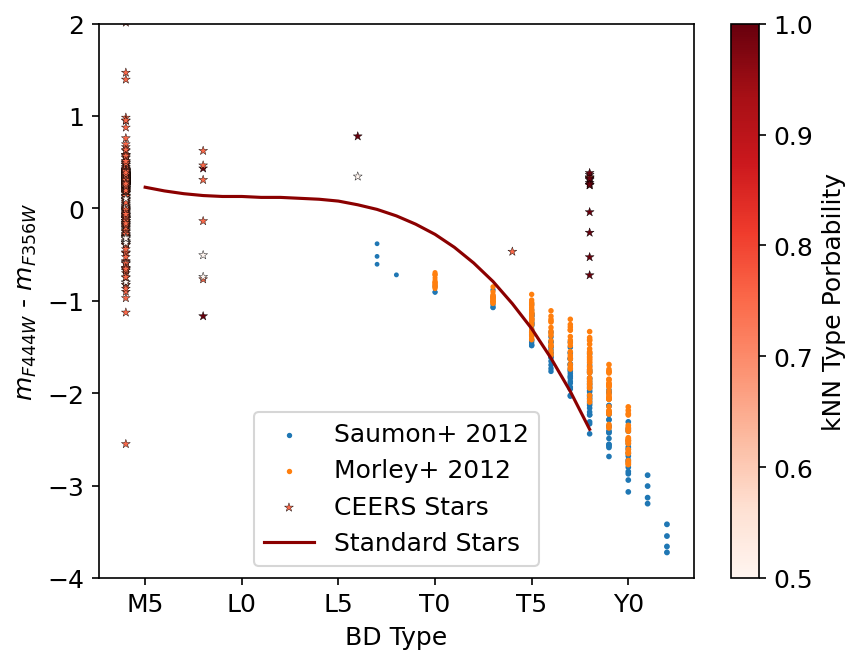
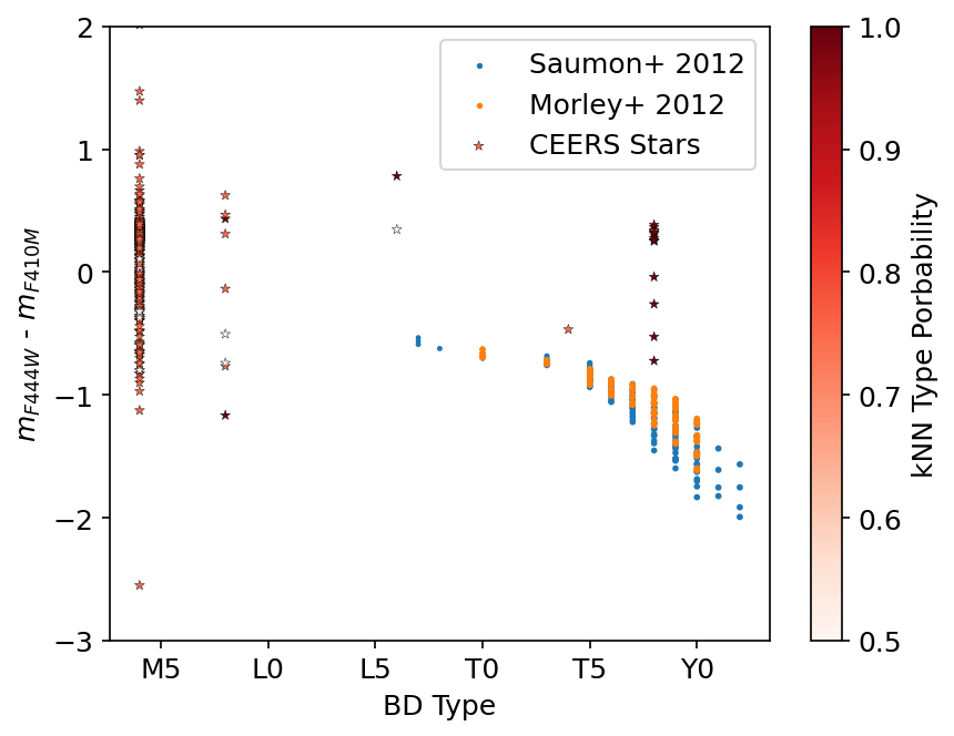
Figure 17: The kNN assigned brown dwarf type against the F444W-F356W and F444W-F410M colours. The dark red line is the W1-W2 WISE colour of standard stars as a function of type.

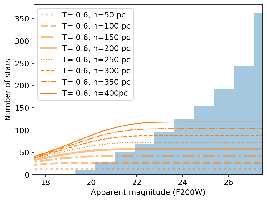
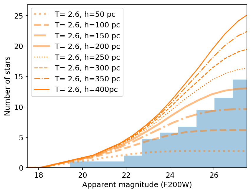
Figure 18: The cumulative histogram of apparent magnitude in F200W for the kNN identified types T=M6$\pm$2 and T=T6$\pm$2 and the expected distribution assuming this type and different Galactic vertical scale-heights.

5.3 blackNIRSpec prism observations

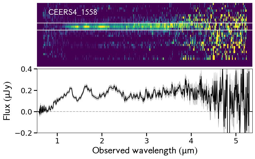
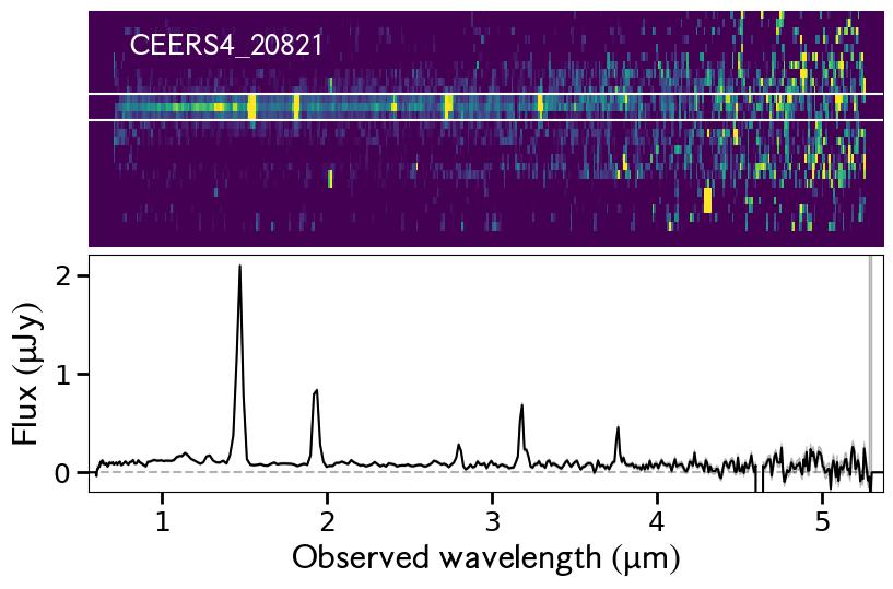
Figure 19: NIRSpec prism spectra of two of the unresolved objects identified by the kNN classification method. The 2D spectra are shown above, with the extraction window marked with a white border. The 1D extracted spectra are shown below. Left: CEERS NIRSpec MSA ID #1558 shows broad absorption bands at 1.5, 2 and 2.5 microns typical of later type brown dwarfs (see Figure 4). Right: CEERS NIRSpec MSA ID #20821 is a galaxy at $z=1.94$ with strong emission lines that perturb the NIRCam photometry, leading to misclassification as a brown dwarf.

blackTwo of the kNN brown dwarf candidates were ob0served with CEERS NIRSpec Multi-Shutter Assembly (MSA) spectroscopy (Arrabal Haro et al., in prep.) using the low-resolution ($R=30$–300) prism disperser (Figure 19). These targets were not originally selected to be stars, but as candidates for distant extragalactic objects.

blackCEERS object black53250 (NIRSpec MSA ID 1558) was originally selected as a NIRSpec target from HST CANDELS data as candidate for a galaxy with photometric redshift $z>6$. Fitting galaxy spectral energy distribution models to the NIRCam and HST photometry yields a photometric redshift sharply peaked at $z\sim 8$ due to the flux discontinuity at $\sim$1$\mu$m. However, this photometric redshift goodness-of-fit is very poor ($\chi^{2}=240$), and there is a very significant detection in the HST F814W filter, which is inconsistent with a Ly$\alpha$ break at $z\sim 8$. The stellar kNN classification for is T=0.4 (M4) and T=0.8 (M8) with 50% probability ($P(T=0.4)=50$% and $P(T=0.8)=50$% ). The spectrum shows the characteristic absorption features at 1.5 and 2.5 microns typical of a later L- or early T-type (e.g., L4 t0 T2) ultracool dwarf, based on a visual inspection. This is somewhat inconsistent with the confusion matrix of the kNNs (Figure 12) where later types are more commonly mis-classified as early-type brown dwarfs.

blackCEERS object 22148, with apparent magnitude $m_{F200W}=26.09$AB and half-light radius $r_{eff}=0\aas@@fstack{\prime\prime}08$, sits just below the stellar locus identified in Figure 2. Although it was not included in the “stellar” object catalog in Table 1, we investigated it because it was observed with NIRSpec. The kNN classification for this object is M4/8 with 75/25% probability ($P(T=0.4)=75$% and $P(T=0.8)=25$%). It was selected as a NIRSpec target (NIRSpec MSA ID 20821) from HST CANDELS data as a candidate galaxy with photometric redshift $z\approx 1.92$. That identification is confirmed by the NIRSpec spectrum, which shows strong emission lines at $z=1.94$ from the Hydrogen Balmer and Paschen series, [OIII]4960,5008, [SIII]9533, and He I 10833. The emission lines contribute significantly to fluxes measured through the NIRCam filters, perturbing the colors and leading to the photometric misclassification as a cool star. This object serves as an important reminder that individual kNN identified objects are primarily candidates until spectroscopically confirmed, and that careful selection of unresolved objects can aid in the precision of the selected sample. Fortunately, a probabilistic Milky Way model can cope with a certain amount of contamination. For example, the MCMC model from van Vledder et al. (2016) accounted for 40% misclassification.

5.4 Scale-height of Brown Dwarfs

blackTo model the scale-height of the Galactic disk along the one line-of-sight of the CEERS field, we use the cumulative count of brown dwarfs as a function of apparent magnitude (similar to Pirzkal et al., 2005, 2009). Assuming a brown dwarf type and the local density blackwithin 20 parsec from Reid et al. (2008) and Kirkpatrick et al. (2021) and a scale-height, one can compute the numbers of brown dwarfs along the line-of-sight. This works best with a single brown dwarf type, a cleanly selected sample, and only the thin disk of the Milky Way considered.

Figure 18 shows two cumulative histograms of the brown dwarf candidates identified in CEERS. The early types (T=0.6, i.e. M6) show an over-density compared to the thin disk. blackAt the lower apparent luminosities, there is a clear over-density that cannot be explained by a Galactic thin disk alone. This is similar to what Holwerda et al. (2014a) and van Vledder et al. (2016) found for M-dwarfs in the HST pure-parallel fields. The cumulative histogram is consistent with a thin disk with a scale-height of $z_{0}=250-300$pc, similar to the scale-heights found before (Ryan et al., 2005, 2011; Pirzkal et al., 2005, 2009; Holwerda et al., 2014b; van Vledder et al., 2016; Aganze et al., 2022b). A second Galactic structural component is needed to explain the numbers of M-dwarfs in deep JWST/NIRCam fields.

The second panel of Figure 18 shows the distribution of late dwarfs (T=2.6, i.e. T6$\pm$2). Their distribution is mostly consistent with a thin disk alone as they are intrinsically much fainter ($M_{J}=17.06$AB). blackA second component is not fully evident from the counts in CEERS. The cumulative histogram is consistent with a thin disk with a scale-height of $z_{0}=150-200$pc, similar to the scale-height of 175pc found before (Ryan et al., 2011; Aganze et al., 2022b).

There is the matter of types in-between the early and late brown dwarfs apparently missing in this field. There are two L-dwarfs and one early T-dwarf in this field with reasonably high confidences. This is not yet enough statistics to infer a scale-height with much confidence. To infer scale-heights accurately, one will need many more lines-of-sight though the Milky Way disk.

6 Discussion

JWST opens up a new parameter space in the near-infrared, thanks to both more collecting area and much improved efficiency compared to other NIR observatories. CEERS is meant to demonstrate this potential, especially in extra-Galactic science. However, the depth and colour resolution that benefits extra-galactic science can benefit science examining our own Milky Way’s stellar population just as much.

Figure 2 illustrates the first improvement: the identification of stellar objects in drizzled NIRCam images increases from HST ($\sim 25$) to $\sim$28AB mag using otherwise identical techniques. This alone opens a wide volume of the Galaxy for low-mass stellar objects.

The much greater filter suite available onboard NIRCam is a second capability that expands our discovery space over HST/WFC3. The bluest NIRCam filters combine into a similar feature space (Figure 7 compared to Figure 8) but the addition of longer wavelength information with NIRCam immediately allows us to check kNN classifications. For these colors atmosphere models can stand in for the SPLAT observations (see Appendix A) but performance is not quite as reliable as SPLAT. This can be attributed to the much larger training sample in SPLAT ($\sim$1200) over these models ($\sim$300) which captures the range of characteristics inherent in the population. The models however extend to later types of brown dwarfs and cover longer wavelengths, opening up the possibility to train on models and then use the full NIRCam wavelength range to classify stellar objects.

The late-type candidates for example appear to have too blue colours in the reddest NIRCam filters (Figure 17). This could be mis-identification or an issue with calibration of the kNN. The effect is quite pronounced and could speculatively be explained by more sulfur and phosphorus compounds in these substellar objects (Figure 4).

black The F444W-F356W colours of the brown dwarfs are very similar to the F200W dropout galaxies identified in Bisigello et al. (2023), their figure 4 (see Figure 20) blackbut with F200W and bluer detections. The accurate identification of brown dwarfs is therefore critical in the removal of potential interlopers in the identification of new (low redshift) dwarf galaxy populations ($z<2$). Similarly, some kNN identified late-type ultracool dwarfs reside in the HST-dark section of the colour space identified in Pérez-González et al. (2023). These authors took care to select these samples using other colour cuts and SED fits. Figure 20 illustrates the possibility that brown dwarfs could be included without such precautions. In such cases, a high probability assigned by the kNN classifier that the unresolved object is a brown dwarf may be a good reason to remove an object from a selection.

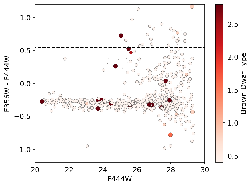
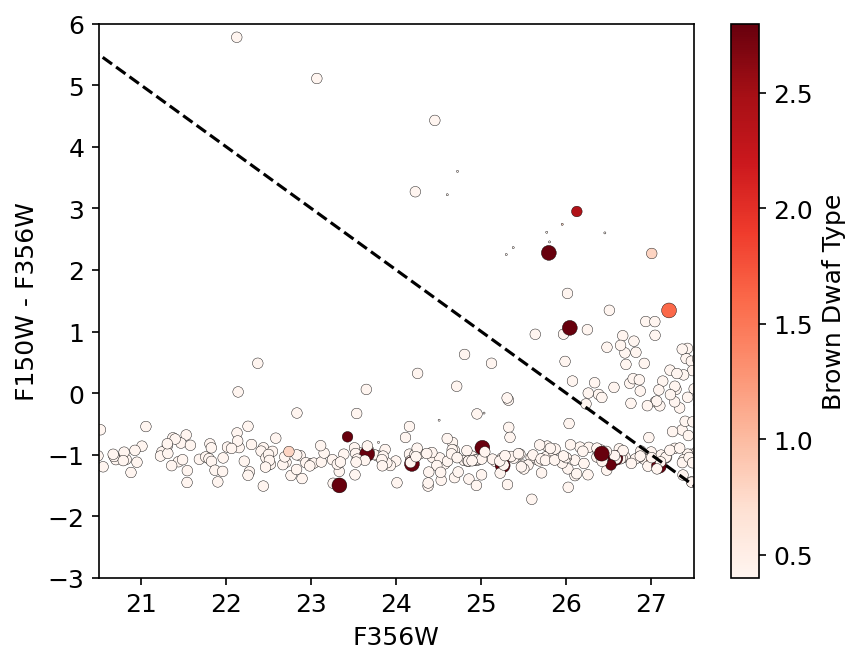
Figure 20: A comparison to Figure 4 of Bisigello et al. (2023) and Figure 1 from Pérez-González et al. (2023) for the kNN classified stellar objects. blackMarker size is indicative of the kNN probability assigned to each object’s classification. The dashed lines are the lower limits for the selection criteria for dusty dwarfs (left) or HST-dark galaxies (right). Both populations can suffer from contamination from brown dwarfs.

black A major consideration in the successful identification of brown dwarfs in extra-galactic JWST data is to remove them as contaminant in searches for high-redshift sources ($z>8$) Figure 21 shows the bluer NIRCam colours of the brown dwarfs identified with kNN and the high-redshift sources from Finkelstein et al. (2023). The $z>12$ sources are dropouts in the F115W and therefore not shown in the bluest colour F115W-F150W. Both the high-redshift sample and the brown dwarf kNN selection do not rely on hard colour criteria but instead on good SED fits to a template and redshift or a close set of kNN templates in colour space.

blackFigure 21 illustrates that a colour-cut in F115W-F150W can separate the two popylatins well but that the redder NIRCam colours are very similar for brown dwarfs and high-redshift galaxies alike.

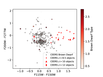
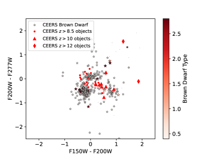
Figure 21: The F115W-F150W and the F150W-F200W vs F200W-F277W colours of the brown dwarf candidates identified in this paper and the same colours of the Finkelstein et al. (2023) selection of high ($z>8$) redshift galaxies.

black Photometric identification of brown dwarfs in JWST data is ongoing (Nonino et al., 2023; Beiler et al., 2023; Wang et al., 2023). Like all photometric identifications, the kNN classifications here would benefit from spectroscopic confirmation using NIRSpec. Figure 19 shows a first such spectroscopic confirmation with a low-resolution NIRSpec prism spectrum. This would be the second ultracool brown dwarf spectroscopically confirmed with JWST after Beiler et al. (2023).

black Wang et al. (2023) identify a T dwarf in the public CEERS data. This object is not in our kNN classified sample as it too faint to be included ($m_{F200W}=28.45$AB, see Figure 2). However, a kNN classification trained on just the blue JWST/NIRCam filters (F115W, F150W, F200W, and F277W) predicts a L7 dwarf ($T_{eff}=1530$K, $P_{kNN}(Type)=100$%), a higher effective temperature than ($T_{eff}=1300$, T0 a)s classified by Wang23e. The reported F444W-F356W colour (-0.14) is consistent with the kNN classification as well as the Wang et al. (2023) one (Figure 17). We can note here that L7 and T0 are less than 4 subtypes apart.

blackThe difference between kNN classification and spectroscopic classification for individual sources highlights the statistical nature of the kNN classifications. It shows that kNN classifications are good enough for a population of sources to be used in a statistical manner to infer the shape of the Milky Way. An MCMC model such as employed by van Vledder et al. (2016) has the benefit of explicitly dealing with a fraction of the data as bad as a fit parameter.

The inferred vertical profiles of M and T-dwarfs is 300-350pc for the $M6\pm 2$ dwarf candidates in the CEERS field with a clear second component starting at $m_{F200W}\sim 24$ in Figure 18. This is consistent with what van Vledder et al. (2016) found for HST/WFC3 pure-parallel fields (300pc). The scale-height of the candidate T-dwarfs is more consistent with 150-200pc. This is remarkably consistent with what Aganze et al. (2022b) found from HST grism observations (175pc).

The photometric identification of M-L-T-Y dwarf stars in deep extragalactic observations such as CEERS has a success rate (85% or better) with existing photometry. It seems only a matter of time before enough sightlines through the Milky Way will be available for an accurate assessment of their distribution and total numbers.

7 Conclusions

We have applied kNN identificataion of brown dwarf types on the unresolved sources in the stellar locus of CEERS photometry with the aim of identifying this Galactic population

Broad filters onboard JWST/NIRCam are sufficient to identify brown dwarfs photometrically to within 2 subtypes using k-Nearest Neighbour classification using the four nearest neighbours. We only use the four bluest filters for this (F115W, F150W, F200W and F277W). The SPLAT library is optimal as a training set with sufficient size and coverage of type. Conceivably atmospheric models of M-L-T-Y dwarfs may replace these as the training set.

The late-type brown dwarfs identified in CEERS are bluer in the NIRCam red filters than expected on the kNN classification based on NIR blue filters. This remains unexplained by standard stars or atmospheric models.

The scale height of the MW disk is consistent with the 350 pc for type M-types, similar to what van Vledder et al. (2016) found. The vertical distribution of later T-types is consistent with a scale-height of 150-200pc, in line with the value from Aganze et al. (2022b).

Data Availability

CEERS is committed to data-releases. This work is based on the data released in the first public data-release. See the CEERS website for details: https://ceers.github.io/releases.html.

Appendix A Models

We test the kNN classifier based on the models from Saumon et al. (2012) and Morley et al. (2012). In total 337 different models are available. Figure 22 shows the colour feature space. Brown dwarf type was assigned to each model using the table from Pecaut & Mamajek (2013) matching model temperature to a brown dwarf type with similar temperature. This is not as big a training set as the SPLAT catalogue.

Figure 24 shows the confusion matrix of the models. Like the SPLAT catalogue, there is a tendency for the kNN to classify brown dwarfs slightly later. Coverage of type is not as uniform as SPLAT and this hinders interpolation with kNN some. The performance as a function of type resolution is shown in Figure 23 and this lack of coverage is evident in an erratic increase in most metrics.

There are two major benefits of these models over the SPLAT catalog: first the feature space includes the red NIRCam filters as well. One can use all the NIRCam photometry to classify. Secondly, the models extend to much later types than SPLAT. Future suites of models black(e.g. improved line lists, disequilibrium chemistry, improved treatment of clouds etc.), once verified with spectroscopy, could well serve as the training set for future kNN classifications.

Figure 22: The colour-colour feature space from the models of Saumon et al. (2012) and Morley et al. (2012). The type space is a few late L-type, most T-types and early Y-type. The full feature space does include all CEERS filter colour combinations.

Figure 23: The performance of the kNN using the colours based on the models of Saumon et al. (2012) and Morley et al. (2012). The higher dimensionality but lower type coverage results in some erratic behavior.

Figure 24: The confusion matrix of the kNN model based on the colours based on the models of Saumon et al. (2012) and Morley et al. (2012). Compared to the SPLAT confusion matrix in Figure 11.

ID	T	P(T)	RA	DEC	$m_{606}$	$m_{814}$	$m_{105}$	$m_{125}$	$m_{140}$	$m_{160}$	$m_{115}$	$m_{150}$	$m_{200}$	$m_{277}$	$m_{356}$	$m_{410}$	$m_{444}$
230	0.4	0.75	215.005725	53.019548	28.2	27.9	…	…	26.6	…	27.0	26.9	27.3	27.6	28.0	28.4	28.6
442	0.4	0.75	214.984572	53.003732	28.0	28.0	…	…	…	…	27.9	28.0	27.9	27.8	27.4	28.1	28.0
471	0.4	0.75	215.008698	53.019115	22.4	20.5	…	19.6	19.4	19.3	19.5	19.3	19.4	20.1	20.3	20.3	20.5
1056	0.4	0.75	214.979593	52.996941	28.0	27.5	…	27.3	28.1	27.9	27.7	27.5	26.8	27.2	28.0	27.9	27.7
1273	0.4	0.75	214.988092	53.002487	27.1	26.8	…	…	27.2	…	26.8	26.9	26.9	26.8	27.0	27.3	27.3
1411	0.4	0.75	214.989956	53.002400	26.2	24.9	…	23.7	23.5	23.6	23.4	23.3	23.5	24.0	24.3	24.4	24.6
1576	0.4	0.75	214.960103	52.980446	26.9	25.2	…	24.7	24.7	24.7	24.5	24.5	24.7	25.1	25.5	25.7	25.8
2021	0.4	0.75	214.930229	52.957510	29.1	27.3	…	27.4	26.5	27.0	26.6	26.5	26.7	27.2	27.5	27.5	27.7
2237	0.4	0.75	214.985580	52.995560	28.6	28.1	…	27.8	28.0	27.7	27.8	27.8	27.9	28.4	29.0	30.0	28.9
2282	0.4	0.75	215.002842	53.007589	30.9	…	…	28.1	…	27.5	28.2	28.1	27.9	27.9	26.9	26.3	26.3
2621	0.4	0.75	215.002406	53.005436	27.0	26.2	…	25.7	25.6	25.7	25.7	25.6	26.0	26.4	26.8	27.0	27.0
2651	0.4	0.75	214.940836	52.961364	22.5	21.8	…	21.7	21.8	21.6	21.6	21.5	21.8	22.4	22.9	23.1	23.3
2962	0.4	0.75	214.957929	52.972366	25.6	24.5	…	24.0	24.0	24.0	24.0	23.9	24.1	24.6	24.9	25.1	25.2
3078	0.8	0.50	214.950840	52.966864	28.9	29.0	…	…	30.1	27.9	28.6	28.7	27.6	26.3	26.0	25.6	25.4
3180	0.4	0.75	214.935770	52.955376	25.5	22.5	…	21.0	20.9	21.0	20.9	20.9	20.9	21.4	21.5	21.6	21.8
3288	0.4	0.75	215.001017	53.001658	22.6	21.4	…	20.8	20.7	20.7	20.7	20.6	20.9	21.4	21.7	21.8	22.0
3422	0.4	0.75	215.003532	53.001914	27.1	26.8	…	27.2	27.4	27.0	26.9	27.1	27.1	27.0	27.3	27.4	27.6
3726	0.4	0.75	214.934274	52.951894	28.3	27.2	…	26.2	26.5	26.1	26.1	26.0	26.3	26.7	27.0	27.2	27.3
3766	0.4	0.75	214.950836	52.963328	28.8	28.3	…	28.2	29.4	28.6	28.2	28.8	27.8	28.2	29.2	33.4	29.1
4144	0.4	0.75	214.992723	52.990798	23.8	22.7	…	22.2	22.0	22.1	22.0	21.9	22.0	22.6	22.9	23.0	23.2
4190	0.4	0.75	215.013710	53.005715	29.2	28.6	…	…	…	28.4	29.0	28.7	27.9	28.4	29.3	29.5	29.1
4587	0.4	0.75	214.964290	52.968574	24.3	22.4	…	21.6	21.6	21.6	21.7	21.6	21.7	22.3	22.4	22.5	22.7
5264	0.4	0.75	214.992931	52.985541	27.8	27.5	…	27.5	27.1	26.8	27.3	26.8	27.1	27.4	27.4	27.5	27.5
5691	0.4	0.75	214.994130	52.982790	27.7	26.3	…	25.5	25.7	25.5	25.5	25.4	25.7	26.2	26.5	26.6	26.6
5715	0.4	0.75	214.962876	52.959907	25.4	23.4	…	21.6	21.3	21.3	19.2	19.1	19.3	20.2	20.2	20.2	20.5
5834	0.4	0.75	214.975604	52.967702	26.0	22.8	…	20.9	20.9	20.9	20.7	20.6	20.8	21.3	21.4	21.4	21.6
6027	0.4	0.75	215.014267	52.995323	26.1	25.2	…	24.7	24.7	24.7	24.6	24.6	24.8	25.3	25.6	25.8	26.0
6218	0.4	0.75	215.029587	53.004863	25.2	24.1	…	20.9	…	20.8	19.7	19.6	19.8	20.5	20.7	20.8	21.0
6246	0.4	0.50	214.973814	52.965578	28.5	28.8	…	29.2	29.1	28.5	29.0	28.8	27.9	29.4	29.0	29.1	28.8
6258	0.4	0.75	215.025600	53.003775	28.1	27.2	…	27.7	…	26.6	26.6	26.5	26.7	27.3	27.6	27.4	28.0
6330	0.4	0.75	214.979867	52.969340	25.1	22.9	…	22.1	22.2	21.9	21.6	21.6	21.8	22.3	22.7	22.8	23.0
6337	0.4	0.75	214.957941	52.953703	28.1	28.1	…	28.4	28.2	29.0	27.9	27.2	27.7	28.6	28.6	29.8	28.6
6483	0.4	0.75	215.032615	53.005980	…	28.5	…	25.9	…	25.7	25.9	25.6	25.6	25.9	25.1	24.9	25.3
6489	0.4	0.75	215.016728	52.994335	24.3	22.5	…	21.7	21.7	21.7	21.7	21.6	21.8	22.3	22.5	22.6	22.8
6717	0.4	0.75	214.950411	52.946651	23.0	22.6	…	22.6	22.7	22.7	22.7	22.6	22.9	23.5	24.0	24.2	24.4
6898	0.4	0.75	214.962186	52.954163	23.0	22.8	…	22.9	23.0	23.1	22.9	23.1	23.4	24.0	24.5	24.8	24.9
6911	0.4	0.75	214.949781	52.945927	29.6	26.9	…	25.7	25.7	25.7	25.3	25.3	25.6	26.0	26.2	26.2	26.4
6973	0.4	0.75	214.969216	52.958760	28.8	28.4	…	27.6	27.8	27.6	27.7	27.4	27.1	26.9	26.9	26.9	26.8
7545	0.4	0.75	214.955399	52.949592	28.4	28.4	…	28.2	…	29.1	28.7	28.5	27.7	28.5	29.1	28.3	29.0
7717	0.4	0.75	215.024715	52.994340	30.3	27.8	…	29.1	…	27.6	27.7	27.8	27.7	26.5	27.8	26.6	27.0
8126	0.4	0.75	215.017125	52.987062	28.1	27.2	…	26.4	26.7	26.4	26.2	26.1	26.3	26.8	27.2	27.3	27.5
8515	0.4	0.75	215.035650	52.998044	28.2	28.4	…	28.9	…	27.9	28.0	27.1	27.9	29.1	29.0	…	31.7
8530	0.4	0.75	215.020822	52.987341	28.1	24.7	…	23.6	23.8	23.6	23.3	23.2	23.4	23.9	24.2	24.3	24.4
8575	0.4	0.75	215.022248	52.988222	29.0	26.8	…	25.5	25.5	25.5	25.2	25.2	25.5	25.9	26.0	26.1	26.4
9029	0.4	0.75	214.980744	52.956755	30.8	28.1	…	27.5	26.6	27.3	27.4	27.4	27.5	28.0	28.0	28.5	28.3
9127	0.4	0.75	214.982252	52.957187	28.4	28.3	…	28.0	…	29.4	28.6	28.3	27.6	27.9	28.8	28.1	28.0
9589	0.4	0.75	214.974717	52.949398	…	…	…	27.7	27.6	27.8	27.5	27.6	27.7	27.6	26.7	27.2	27.6
9770	0.4	0.75	214.969556	52.944876	28.9	28.1	…	27.3	29.1	27.3	27.6	27.6	27.8	28.3	28.7	28.5	28.7
9777	0.4	0.75	214.985683	52.956235	…	27.1	…	27.9	27.4	27.6	27.2	27.3	27.2	25.9	26.7	25.4	25.7
9871	0.4	0.75	215.029971	52.987114	29.8	28.3	…	27.5	27.1	27.6	27.3	27.3	27.5	28.0	28.2	28.5	28.5
9894	0.4	0.75	215.046316	52.997842	28.5	28.5	…	28.0	…	27.7	28.0	27.7	27.7	27.7	27.6	27.6	27.6
10176	0.4	0.75	214.979196	52.949329	25.6	24.5	…	24.2	24.1	24.1	23.9	23.9	24.0	24.5	24.9	25.1	25.2
10223	0.4	0.75	214.960701	52.936021	28.4	28.5	…	29.2	28.2	28.6	28.7	28.1	27.7	28.7	28.8	28.1	28.4
10398	0.4	0.75	214.958571	52.935659	29.0	28.6	…	28.8	29.8	28.6	28.8	28.4	27.8	29.2	28.8	29.1	28.6
10891	0.8	0.75	214.881159	52.930636	29.2	29.0	…	28.3	28.1	28.1	29.2	28.7	27.9	28.4	29.2	28.1	28.4
11280	0.4	0.75	214.850554	52.910358	27.0	…	…	…	…	…	29.7	…	27.5	30.3	28.6	30.1	31.0
11534	0.4	0.75	214.863670	52.915518	27.8	28.1	…	28.0	…	27.8	28.0	28.0	27.3	27.4	28.6	28.9	28.2
11681	0.4	0.75	214.895567	52.937328	…	25.6	…	23.7	23.7	23.8	23.6	23.6	23.7	24.2	24.2	24.2	24.4
12051	0.4	0.75	214.917207	52.950931	27.4	26.1	…	25.7	25.7	25.7	25.7	25.7	25.9	26.4	26.7	26.9	27.0
12452	0.4	0.75	214.911604	52.945046	28.2	28.4	…	27.8	28.0	27.5	28.2	27.4	27.9	29.0	28.5	28.9	29.1
12539	0.4	0.75	214.911117	52.944318	28.4	27.3	…	26.8	26.4	27.2	26.9	26.9	27.1	27.5	27.9	27.9	28.3
12566	0.4	0.75	214.894569	52.932425	32.8	28.4	…	27.2	29.7	28.0	27.5	27.4	27.7	27.9	27.9	27.5	28.0
13791	0.4	0.75	214.842350	52.889154	24.3	24.1	…	24.0	24.1	24.3	23.5	23.8	24.3	24.8	25.3	25.5	25.7

Table 3: – continued

ID	T	P(T)	RA	DEC	$m_{606}$	$m_{814}$	$m_{105}$	$m_{125}$	$m_{140}$	$m_{160}$	$m_{115}$	$m_{150}$	$m_{200}$	$m_{277}$	$m_{356}$	$m_{410}$	$m_{444}$
14111	0.4	0.75	214.866930	52.904939	26.2	25.3	…	24.6	24.7	24.6	24.6	24.5	24.8	25.2	25.6	25.7	25.9
14129	0.4	0.75	214.910007	52.935116	28.1	27.7	…	27.6	28.1	27.5	27.6	27.6	27.5	27.5	27.9	28.0	28.1
14185	0.4	0.75	214.876678	52.911429	…	28.9	…	27.3	28.0	27.1	27.4	27.6	27.7	27.9	27.8	27.7	28.1
14865	0.4	0.75	214.880989	52.910540	30.3	29.0	…	28.6	28.0	27.9	28.4	28.2	27.7	27.4	27.4	27.5	27.4
14968	0.4	0.75	214.910169	52.930537	24.4	23.4	…	22.9	22.9	22.9	22.9	22.8	22.9	23.5	23.8	23.9	24.1
15645	0.4	0.75	214.930282	52.941671	27.8	26.5	…	25.8	26.3	25.9	25.9	25.8	26.1	26.5	26.9	27.1	27.2
16420	0.4	0.75	214.866867	52.891148	28.5	28.2	…	27.6	27.8	27.8	27.8	27.7	27.6	27.9	28.4	28.6	28.5
16558	0.4	0.75	214.930384	52.936557	28.2	28.4	…	27.7	28.6	28.7	28.4	28.4	27.6	28.2	29.1	…	29.2
16868	0.4	0.75	214.863408	52.886410	28.1	26.6	…	26.0	25.7	25.8	25.5	25.4	25.7	26.2	26.4	26.6	26.7
17386	0.4	0.75	214.858301	52.879705	29.0	28.3	…	28.6	…	28.5	28.5	28.2	27.4	27.9	29.0	28.8	28.2
17887	0.4	0.75	214.863528	52.880377	28.8	28.4	…	28.2	29.0	28.0	28.2	28.0	27.3	27.4	27.5	27.4	27.4
18030	0.4	0.75	214.863422	52.879629	29.1	28.8	…	…	28.0	29.0	28.6	28.8	27.9	27.9	29.0	28.6	28.3
18150	0.4	0.75	214.919686	52.918869	25.2	24.2	…	23.6	23.6	23.5	23.5	23.4	23.6	24.1	24.4	24.6	24.7
18548	0.4	0.75	214.875679	52.885998	26.6	26.5	…	26.4	26.3	26.2	26.1	26.1	26.2	26.2	26.2	26.1	26.2
18638	0.4	0.75	214.880253	52.888485	27.9	27.6	…	27.5	27.8	27.9	27.8	28.0	27.8	27.7	27.8	27.9	28.2
18658	0.4	0.75	214.884064	52.890967	25.6	25.2	…	25.7	25.7	25.7	25.7	25.5	25.6	25.5	26.0	26.2	26.0
18968	0.4	0.75	214.924041	52.917899	28.4	28.6	…	28.0	27.7	29.1	28.9	28.6	27.8	28.3	29.1	28.5	28.5
18981	0.4	0.75	214.864028	52.877402	26.5	25.2	…	24.6	24.5	24.5	24.2	24.1	24.3	24.8	25.2	25.3	25.5
19085	0.4	0.75	214.868228	52.877616	27.7	26.9	…	26.3	26.2	26.2	26.2	26.0	26.3	26.8	27.4	27.6	27.5
19149	0.4	0.75	214.943750	52.930901	29.1	27.9	…	26.6	26.6	27.0	25.8	26.0	26.5	27.0	27.5	27.7	27.7
19200	0.4	0.75	214.930694	52.921178	23.4	22.5	…	22.0	22.0	21.9	21.9	21.8	22.0	22.6	22.9	23.1	23.3
19498	0.4	0.75	214.889424	52.890607	24.4	23.2	…	22.4	22.4	22.3	22.3	22.2	22.4	22.9	23.2	23.4	23.5
19507	0.4	0.75	214.926551	52.916861	28.8	28.4	27.5	28.6	28.3	28.5	28.3	28.3	27.6	27.7	27.6	27.5	27.6
19948	0.4	0.75	214.922775	52.911761	27.5	26.2	…	25.8	26.2	25.7	25.7	25.5	25.8	26.3	26.6	26.7	26.9
19984	0.4	0.75	214.872559	52.875948	…	28.7	…	28.1	27.3	28.4	27.8	28.0	27.9	27.8	27.0	28.5	27.4
20040	0.4	0.75	214.926775	52.914039	30.5	27.5	27.8	26.8	26.9	27.0	26.8	26.9	26.7	25.6	26.7	25.6	26.2
20105	0.4	0.75	214.876732	52.877794	26.5	24.1	…	23.2	23.2	23.3	23.0	23.0	23.1	23.7	23.9	23.9	24.1
20188	0.4	0.75	214.958561	52.935652	28.6	28.2	…	28.4	28.7	28.1	28.3	28.2	27.4	28.0	28.7	28.1	28.6
20442	0.4	0.75	214.899367	52.891983	25.6	24.4	…	23.9	23.9	23.8	23.9	23.7	23.9	24.4	24.8	25.0	25.1
20928	0.4	0.75	214.764897	52.852763	28.4	29.1	…	…	…	…	27.7	27.3	27.4	27.6	28.4	27.6	28.3
21058	0.4	0.75	214.736375	52.831994	28.0	26.3	…	25.7	…	25.6	25.6	25.6	25.8	26.4	26.6	26.9	26.9
21160	0.4	0.75	214.802546	52.877954	28.2	27.5	…	…	27.5	…	26.9	26.9	27.0	27.4	27.9	27.8	28.1
21352	0.4	0.75	214.763509	52.848842	26.0	26.0	…	25.3	…	26.8	25.8	26.5	26.6	26.1	26.3	26.2	25.8
21378	0.4	0.75	214.754038	52.841925	27.8	26.3	…	25.7	…	25.6	25.8	25.6	25.8	26.3	26.6	26.8	26.9
21419	0.4	0.75	214.795683	52.871054	27.8	27.4	…	27.2	26.9	26.8	27.0	26.8	26.9	27.5	28.0	28.2	28.6
21453	0.4	0.75	214.805767	52.878048	30.4	28.8	…	30.4	27.2	38.4	27.4	27.6	27.6	27.5	27.2	27.0	26.1
21635	0.4	0.75	214.805093	52.877077	28.0	25.5	…	26.9	24.2	31.2	23.8	23.9	24.2	24.7	24.7	24.8	24.9
21879	0.4	0.75	214.795393	52.868700	28.0	25.0	…	23.7	23.7	23.6	23.4	23.4	23.6	24.0	24.1	24.2	24.4
21961	0.4	0.75	214.750864	52.836555	27.8	27.7	…	27.7	27.0	26.7	27.5	26.7	26.8	27.8	27.4	27.6	27.9
22090	0.4	0.75	214.771338	52.850158	28.2	28.8	…	28.0	…	30.0	28.2	28.1	27.7	28.1	28.5	27.9	28.1
22144	0.4	0.75	214.818006	52.882991	30.2	26.9	…	23.4	23.4	23.1	23.4	22.9	22.6	23.0	22.4	22.3	22.7
22303	0.4	0.75	214.809475	52.878209	22.8	22.4	…	22.2	22.2	22.1	22.4	22.1	22.3	22.9	23.3	23.6	23.7
22357	0.4	0.75	214.752488	52.835521	28.9	29.7	…	28.9	…	27.6	28.6	27.4	27.9	27.3	27.9	27.3	28.0
22422	0.4	0.75	214.755244	52.836789	22.4	22.2	…	22.0	22.0	22.0	22.2	22.2	22.2	22.0	22.1	22.0	21.8
23077	0.4	0.75	214.807327	52.871140	25.2	22.8	…	21.5	21.8	21.6	21.5	21.5	21.7	22.1	22.3	22.4	22.6
23467	0.4	0.75	214.798219	52.862919	27.0	27.2	…	27.0	27.1	27.2	27.2	27.2	27.3	26.7	27.6	27.5	27.7
23687	0.4	0.75	214.750799	52.828382	27.7	26.8	…	26.4	26.5	26.5	26.4	26.4	26.6	27.1	27.5	27.9	27.8
23948	0.4	0.75	214.829978	52.883291	26.8	24.2	…	22.1	22.1	22.0	21.8	21.7	21.8	22.3	22.3	22.3	22.5
23978	2.4	0.75	214.759819	52.833414	29.7	29.8	…	…	27.1	28.3	29.7	29.1	27.6	26.3	26.1	25.8	25.7
23997	0.4	0.75	214.779962	52.847573	26.7	26.7	…	26.5	…	26.4	26.5	26.4	26.4	26.3	26.4	26.4	26.3
24402	0.4	0.75	214.755275	52.828278	28.8	30.8	…	28.0	29.7	29.1	28.4	28.1	27.7	28.2	28.7	28.5	28.4
24802	0.4	0.75	214.772108	52.838352	29.3	26.7	…	25.1	25.0	25.3	24.7	24.8	24.9	25.4	25.3	25.4	25.6
25196	0.4	0.75	214.780226	52.842028	27.9	28.1	…	27.2	…	27.0	27.3	26.9	27.0	27.0	27.1	27.0	27.0
25376	0.4	0.75	214.836621	52.881916	24.6	22.3	…	21.5	21.5	21.4	21.2	21.1	21.3	21.8	22.0	22.1	22.3
25425	0.4	0.50	214.766576	52.831524	29.2	28.6	…	28.0	27.5	28.1	28.4	28.4	27.0	25.7	25.8	25.5	25.4
25469	0.4	0.75	214.818863	52.868372	27.7	26.5	…	26.1	…	25.7	25.8	25.7	25.9	26.4	26.6	26.7	26.9
25608	0.4	0.75	214.791809	52.847937	22.1	21.0	…	20.5	20.6	20.4	20.4	20.3	20.5	21.0	21.4	21.6	21.7
25936	0.4	0.50	214.763085	52.826315	28.1	28.0	…	28.9	27.9	28.0	28.9	28.7	27.8	28.0	29.5	29.4	28.7
26062	0.4	0.75	214.844147	52.883464	29.6	28.3	…	30.2	27.7	27.9	28.4	28.4	28.0	28.6	28.9	28.8	29.2
26188	0.4	0.75	214.832859	52.874145	28.6	28.2	…	27.7	…	27.8	27.7	27.6	27.6	28.2	28.6	28.9	28.8
26312	0.4	0.75	214.760687	52.823137	23.5	22.5	…	22.0	22.0	22.0	22.0	21.9	22.1	22.6	23.0	23.2	23.3
26362	0.4	0.75	214.818211	52.863636	…	28.1	…	26.9	26.7	27.2	26.6	26.6	26.8	27.3	27.2	27.4	27.6
26436	0.4	0.75	214.824554	52.868856	…	28.1	…	27.2	…	28.2	27.5	27.6	27.7	27.6	26.8	27.9	26.7

Table 1: – continued

ID	T	P(T)	RA	DEC	$m_{606}$	$m_{814}$	$m_{105}$	$m_{125}$	$m_{140}$	$m_{160}$	$m_{115}$	$m_{150}$	$m_{200}$	$m_{277}$	$m_{356}$	$m_{410}$	$m_{444}$
27227	0.4	0.75	214.769238	52.823309	25.6	25.1	…	24.9	24.8	24.8	24.8	24.8	25.0	25.6	26.1	26.3	26.5
27283	0.4	0.75	214.787729	52.836066	24.6	23.5	…	22.9	22.9	22.8	23.1	22.7	22.9	23.4	23.7	23.9	24.1
27458	0.4	0.75	214.766870	52.820418	28.2	26.8	…	26.0	26.6	26.1	26.0	25.9	26.1	26.6	26.9	27.0	27.1
27809	0.4	0.75	214.848625	52.876818	26.9	27.0	…	26.4	26.6	27.0	26.4	26.9	26.9	26.7	26.9	26.8	26.7
27873	0.4	0.75	214.848537	52.876806	27.5	27.5	…	27.0	27.0	27.3	27.0	27.3	27.3	27.2	27.1	27.1	27.1
28165	0.4	0.75	214.823380	52.857420	24.0	23.6	…	23.5	23.4	23.4	23.4	23.3	23.6	24.2	24.7	24.9	25.1
28264	0.4	0.75	214.828982	52.861133	28.0	27.8	…	28.8	27.4	27.4	27.8	27.6	26.9	27.3	27.9	27.9	27.8
28524	0.4	0.75	214.783469	52.827239	23.5	21.7	…	21.3	21.1	20.9	20.9	20.7	20.9	21.5	21.8	21.9	22.1
28875	0.4	0.75	214.790988	52.831064	24.8	24.0	…	23.6	23.6	23.6	23.5	23.4	23.6	24.2	24.6	24.8	24.9
28949	0.4	0.75	214.855951	52.877475	23.0	21.7	…	21.1	21.0	20.9	20.3	20.2	20.3	21.0	21.4	21.5	21.7
29074	0.4	0.75	214.842772	52.867137	25.4	24.2	…	23.6	…	23.5	23.5	23.5	23.7	24.2	24.5	24.7	24.8
29288	0.4	0.75	214.855407	52.875177	28.1	27.2	…	26.9	26.9	26.3	26.2	26.1	26.3	26.8	27.1	27.3	27.5
29328	0.4	0.75	214.802477	52.837146	26.2	24.1	23.2	23.1	23.2	23.0	22.8	22.7	22.9	23.4	23.7	23.8	24.0
29514	0.4	0.75	214.853639	52.872655	28.4	28.8	…	27.9	…	28.2	28.6	28.4	27.8	28.2	29.0	29.0	28.7
29533	0.4	0.75	214.808289	52.839653	22.3	20.8	20.1	20.0	19.9	20.0	19.9	19.8	20.2	20.7	20.9	20.9	21.1
29566	0.4	0.75	214.854415	52.873318	28.4	28.1	…	28.9	…	28.8	28.1	28.5	27.3	27.9	28.8	29.0	28.5
29775	0.4	0.75	214.795038	52.829187	28.2	27.8	…	28.0	27.7	27.8	27.7	27.7	27.9	27.9	27.9	28.3	28.2
29832	0.4	0.75	214.843837	52.863941	23.4	21.7	…	21.1	21.0	21.0	20.8	20.7	20.9	21.6	21.8	21.9	22.1
30183	0.4	0.75	214.846502	52.863074	22.3	21.0	…	19.7	19.8	19.6	19.3	19.1	19.3	19.8	20.3	20.4	20.6
30295	0.4	0.75	214.784186	52.818544	28.0	27.5	…	27.3	27.3	27.2	27.3	27.1	27.0	27.0	27.1	27.3	27.3
30527	0.4	0.50	214.811924	52.837495	30.3	26.4	26.5	24.3	24.4	24.3	24.0	24.1	24.2	24.7	24.5	24.6	24.8
30923	0.4	0.75	214.862778	52.871456	27.2	24.7	…	23.5	23.4	23.4	22.7	22.4	22.6	23.1	23.4	23.5	23.7
31016	0.4	0.50	214.808165	52.832216	29.1	28.9	28.5	28.0	26.8	28.0	28.1	27.8	25.9	24.6	24.6	24.4	24.3
31181	0.4	0.75	214.832537	52.849467	27.5	27.0	26.9	27.2	26.5	26.9	26.7	26.9	26.3	25.4	26.0	25.9	25.6
31216	0.4	0.75	214.785339	52.814935	28.0	27.9	…	28.0	28.1	28.4	27.8	27.6	27.1	28.0	27.7	27.8	28.1
31311	0.4	0.75	214.797221	52.823105	28.3	28.1	…	28.2	28.0	28.5	28.1	28.3	27.5	27.9	28.8	28.9	28.7
31350	0.4	0.75	214.830807	52.846658	23.3	22.5	22.2	22.1	22.1	22.1	22.2	21.9	22.1	22.6	23.0	23.2	23.4
31885	0.4	0.75	214.812584	52.830746	23.1	22.1	21.6	21.7	21.8	21.7	21.4	21.3	21.5	22.3	22.5	22.7	22.8
31897	0.4	0.75	214.782151	52.809273	28.0	27.9	…	27.9	27.5	26.8	27.7	26.8	27.6	28.1	28.0	28.3	28.2
32059	0.4	0.75	214.855453	52.859911	28.5	28.8	…	29.2	28.6	28.8	28.3	27.3	27.0	26.4	26.2	26.1	26.1
32236	0.4	0.75	214.727471	52.773323	31.3	…	…	…	30.6	…	27.7	28.9	27.8	30.3	24.5	28.6	…
32531	0.4	0.75	214.702874	52.752461	25.0	23.5	…	22.8	22.8	23.1	22.7	22.6	22.8	23.3	23.6	23.7	23.9
32607	0.4	0.75	214.720515	52.764802	26.1	25.2	…	24.8	24.7	24.7	24.8	24.6	24.8	25.3	25.7	25.9	26.0
32964	0.4	0.75	214.712783	52.757285	23.1	22.2	…	21.8	21.7	21.6	21.7	21.5	21.7	22.4	22.7	22.8	23.0
33016	0.4	0.75	214.719708	52.762214	26.6	25.3	…	24.8	24.7	24.6	24.7	24.6	24.8	25.3	25.6	25.7	25.9
33054	0.4	0.75	214.766125	52.795290	30.1	28.1	…	27.4	26.9	27.4	26.9	26.9	27.1	27.5	27.7	27.9	28.0
33065	0.4	0.75	214.777152	52.802886	29.1	26.9	…	25.2	25.9	25.0	22.6	22.6	22.7	23.3	23.5	23.6	23.8
33132	0.4	0.75	214.727747	52.773086	22.1	21.3	…	20.9	20.9	20.8	20.8	20.7	20.9	21.5	21.8	22.0	22.2
33241	0.4	0.75	214.765306	52.793781	29.1	28.2	…	27.2	…	28.1	27.4	27.6	27.9	28.1	29.0	28.3	30.4
33296	0.4	0.75	214.755391	52.786329	27.5	27.3	…	26.7	26.8	27.7	26.5	26.9	27.9	27.8	28.2	28.7	27.9
33462	0.4	0.75	214.705061	52.749761	26.8	26.3	…	28.3	28.8	27.8	27.1	27.9	27.3	27.1	26.5	26.7	26.1
33500	0.4	0.75	214.733147	52.769129	25.8	24.9	…	24.5	24.4	24.4	24.5	24.3	24.5	25.1	25.5	25.6	25.8
33532	0.8	1.00	214.701299	52.746152	28.7	28.9	…	27.9	28.2	27.6	28.7	28.4	27.9	28.3	28.9	29.4	29.3
33572	0.4	0.75	214.722424	52.759886	27.1	26.6	…	26.4	26.5	26.3	26.3	26.3	26.1	26.0	26.1	26.3	26.4
33581	0.4	0.75	214.770135	52.795144	27.0	25.7	…	25.4	25.3	25.2	25.1	25.0	25.1	25.7	26.1	26.2	26.4
33592	0.4	0.75	214.722177	52.768643	28.0	27.6	…	27.1	27.1	26.9	27.1	27.0	27.1	26.9	26.8	26.7	26.7
33786	0.4	0.75	214.776136	52.807419	28.3	28.2	…	28.4	27.2	27.2	28.2	27.5	28.0	28.5	28.9	28.5	29.3
33814	0.4	0.75	214.706331	52.748270	27.2	25.3	…	…	…	…	…	…	27.6	28.7	25.6	27.8	27.6
33919	0.4	0.75	214.706865	52.747646	21.6	21.0	…	20.9	20.7	20.7	20.7	20.6	20.8	21.5	21.9	22.1	22.3
33975	0.4	0.75	214.770435	52.793327	22.0	20.4	…	19.7	19.7	19.7	19.7	19.7	19.8	20.6	20.7	20.6	20.8
34101	0.4	0.75	214.754979	52.781467	28.9	26.0	…	24.7	24.8	24.7	24.6	24.6	24.8	25.2	25.3	25.4	25.6
34585	0.4	0.75	214.763531	52.785911	27.4	27.2	…	27.1	27.1	27.1	26.9	26.9	26.8	26.8	27.1	27.4	27.4
34642	0.4	0.75	214.729405	52.760398	24.8	24.1	…	23.8	23.8	23.8	23.8	23.7	23.9	24.5	24.8	25.1	25.3
34765	0.4	0.75	214.727469	52.758484	28.0	28.2	…	28.6	28.1	27.7	28.2	28.2	27.5	27.9	29.0	27.8	28.4
34889	0.4	0.75	214.763797	52.785195	…	28.7	…	…	…	27.8	29.3	27.5	27.8	28.1	28.4	28.2	27.5
35460	0.4	0.75	214.773104	52.787613	29.5	27.3	…	26.2	26.1	26.3	23.3	23.4	23.9	24.3	24.7	24.9	25.0
35603	0.4	0.75	214.780683	52.792263	28.7	28.0	…	27.1	26.7	26.5	27.1	26.6	26.0	25.8	25.6	25.6	25.5
36009	0.4	0.75	214.783152	52.792152	25.4	23.5	…	22.8	22.8	22.8	22.7	22.5	22.7	23.3	23.5	23.6	23.8
36388	0.4	0.75	214.778175	52.786790	28.7	27.4	…	26.7	26.3	26.9	26.1	26.2	26.3	26.8	27.0	27.0	27.1
36653	0.4	0.75	214.723860	52.746207	26.8	25.6	…	24.7	24.6	24.7	24.5	24.3	24.6	25.1	25.4	25.5	25.7
36807	0.4	0.75	214.775079	52.782108	25.6	24.4	…	23.9	23.8	24.0	23.8	23.7	23.8	24.4	24.7	24.9	25.0
36995	0.4	0.75	214.765170	52.773960	27.2	25.6	…	24.9	25.0	24.9	24.9	24.9	25.0	25.5	25.8	25.9	26.1
37180	0.4	0.75	214.773756	52.777408	27.2	26.0	…	25.5	25.4	25.5	25.6	25.5	25.7	26.1	26.5	26.8	26.8
37189	0.4	0.75	214.777634	52.778510	24.2	23.4	…	23.0	23.0	23.0	23.0	22.9	23.1	23.6	24.0	24.2	24.3

Table 1: – continued

ID	T	P(T)	RA	DEC	$m_{606}$	$m_{814}$	$m_{105}$	$m_{125}$	$m_{140}$	$m_{160}$	$m_{115}$	$m_{150}$	$m_{200}$	$m_{277}$	$m_{356}$	$m_{410}$	$m_{444}$
37455	0.4	0.75	214.780023	52.781031	31.3	…	…	…	28.5	29.2	27.4	27.5	27.5	29.8	24.2	…	30.4
38393	0.4	0.50	214.806850	52.795130	28.3	28.4	…	28.0	…	28.0	28.8	28.2	27.4	28.1	29.0	28.8	28.9
38499	0.4	0.75	214.734404	52.742211	28.3	28.4	…	28.7	28.4	28.3	28.3	28.1	27.7	27.9	28.2	28.2	28.1
38545	0.4	0.75	214.720979	52.732671	29.3	27.9	…	27.7	…	27.2	28.2	27.2	27.7	28.0	28.4	28.7	28.7
38589	0.4	0.75	214.729152	52.738314	29.6	27.8	…	27.3	27.3	27.5	27.3	27.2	27.5	27.9	28.2	28.4	28.6
38781	0.4	0.75	214.735560	52.751323	23.3	22.7	…	22.3	22.3	22.3	22.3	22.2	22.4	22.9	23.3	23.5	23.7
39222	0.4	0.75	214.801223	52.786505	27.7	26.9	…	26.4	26.4	26.8	26.3	26.3	26.5	27.0	27.6	27.5	27.6
39627	0.4	0.75	214.732513	52.735163	24.2	22.3	…	20.7	20.7	20.7	20.5	20.5	20.6	21.2	21.3	21.3	21.5
39705	2.8	1.00	214.781488	52.784781	28.3	25.0	…	24.0	23.8	23.9	22.8	22.7	22.9	23.4	23.7	23.8	23.9
40081	0.4	0.75	214.742099	52.758494	28.3	28.3	…	28.1	27.3	26.7	28.0	27.2	27.9	28.6	28.3	28.5	28.9
40417	2.8	1.00	214.782846	52.767735	29.4	28.8	…	28.1	28.4	28.1	28.5	27.9	27.7	27.7	27.7	27.8	27.7
40538	0.4	0.75	214.812487	52.788471	26.6	25.3	…	24.9	24.9	24.8	24.8	24.7	24.9	25.4	25.7	25.9	26.0
40620	0.4	0.75	214.765780	52.754828	29.0	28.9	…	…	27.6	29.1	29.1	28.7	27.9	28.6	29.1	28.7	28.8
41309	0.4	0.75	214.729211	52.735483	27.9	28.5	…	27.8	27.0	27.3	27.8	27.1	27.6	28.0	28.5	28.5	28.6
41397	0.4	0.75	214.757403	52.745288	28.1	27.0	…	25.9	26.6	25.9	25.9	25.8	26.1	26.5	26.9	26.9	27.0
41543	0.4	0.75	214.737662	52.730522	28.7	29.2	…	29.3	27.5	31.0	28.7	28.6	27.8	29.1	29.2	29.0	29.1
41624	0.4	0.75	214.744679	52.734719	28.3	28.2	…	27.8	27.8	27.8	27.8	27.9	27.8	27.8	27.8	27.9	28.2
42403	0.4	0.75	214.769847	52.749194	22.9	22.7	…	22.9	22.9	23.0	22.7	22.9	23.3	23.9	24.4	24.6	24.8
42579	0.4	0.75	214.803161	52.771454	27.3	26.1	26.3	26.0	…	25.9	25.8	25.7	25.9	26.4	26.8	27.0	27.3
43038	0.4	0.75	214.958581	52.930522	22.5	22.1	24.1	22.0	21.9	21.9	21.9	21.8	22.1	22.7	23.3	23.5	23.6
43505	0.4	0.75	214.888239	52.878065	26.0	25.2	…	25.0	25.0	24.8	24.9	24.8	25.0	25.5	26.0	26.2	26.4
43542	0.4	0.75	214.906457	52.890788	29.2	28.1	…	27.7	27.2	27.6	27.3	27.3	27.5	28.1	28.3	29.1	28.5
43555	0.4	0.75	214.962788	52.930411	24.6	22.8	22.1	21.9	22.1	21.8	21.7	21.4	21.6	22.1	22.5	22.6	22.8
43587	0.4	0.75	214.887521	52.876956	25.1	24.2	…	23.7	23.7	23.7	23.6	23.5	23.7	24.3	24.6	24.8	24.9
43767	0.4	0.75	214.960059	52.927440	28.8	28.6	28.3	27.9	28.3	29.8	29.0	28.5	27.9	28.5	29.6	29.7	29.3
44000	0.4	0.75	214.901226	52.884142	25.7	24.9	…	24.5	24.5	24.5	24.5	24.4	24.6	25.1	25.5	25.8	25.9
44149	0.4	0.75	214.901683	52.883576	27.6	27.2	…	27.1	27.2	27.3	27.0	27.1	27.1	27.2	27.3	27.7	27.6
44362	0.4	0.75	214.958897	52.922996	28.2	27.6	27.8	27.8	28.8	28.1	27.5	27.9	27.9	27.9	28.1	28.3	28.3
44429	0.4	0.75	214.907970	52.886471	28.5	28.5	…	27.8	27.8	27.6	27.5	27.2	27.4	27.6	27.6	27.7	27.7
44430	0.4	0.75	214.907748	52.886224	28.6	28.3	…	27.8	28.6	27.9	28.1	27.8	27.9	27.9	27.9	28.0	27.9
44535	0.4	0.75	214.918900	52.893206	27.5	27.3	…	27.3	27.1	27.8	27.0	27.4	27.3	27.3	27.3	27.5	27.7
44572	0.4	0.75	214.898666	52.878853	24.3	22.7	…	22.0	22.1	22.0	22.0	21.8	22.0	22.6	22.8	23.0	23.1
44938	0.4	0.75	214.912258	52.885869	23.6	22.7	…	22.2	22.2	22.1	22.3	22.0	22.2	22.7	23.1	23.3	23.5
45503	0.4	0.75	214.913851	52.884142	24.6	22.6	…	21.6	21.5	21.5	21.5	21.3	21.5	22.1	22.2	22.3	22.4
45542	0.4	0.75	214.909544	52.880950	24.1	23.3	…	22.9	22.9	22.8	23.0	22.8	22.9	23.5	23.9	24.1	24.3
45558	0.4	0.75	214.943679	52.905060	28.6	26.6	24.6	25.7	25.6	25.7	23.6	23.7	24.1	24.6	25.0	25.2	25.3
45597	0.4	0.75	214.957378	52.914447	28.1	27.9	27.8	27.7	28.3	27.9	27.9	27.8	27.7	27.6	27.7	27.9	27.9
45850	0.8	0.50	214.954213	52.910860	29.0	29.0	…	29.4	…	27.8	28.7	28.7	27.8	28.5	29.3	28.1	28.5
45863	0.4	0.75	214.947051	52.905650	27.1	25.9	26.6	25.8	25.4	25.5	25.4	25.3	25.6	26.0	26.4	26.5	26.6
46123	0.4	0.75	214.922420	52.886574	28.4	25.8	…	24.9	24.8	24.9	24.2	23.9	24.2	24.7	24.8	25.0	25.1
46153	0.4	0.75	214.972849	52.922227	28.2	27.3	26.9	26.6	26.5	26.6	26.7	26.6	26.7	27.2	27.5	27.8	27.7
46891	0.4	0.75	214.918623	52.878995	28.8	28.7	…	28.1	27.7	28.7	28.7	28.5	27.6	28.3	28.5	28.3	28.7
47160	0.4	0.75	214.920712	52.877343	30.6	26.2	…	24.0	24.2	23.8	21.9	21.9	22.0	22.5	22.6	22.7	22.8
47201	0.4	0.75	214.904109	52.865473	28.1	27.2	…	27.1	26.5	27.4	26.6	26.4	26.6	27.2	27.4	27.4	27.7
47271	0.4	0.75	214.982109	52.920120	24.3	23.6	23.5	23.4	23.4	23.3	23.4	23.3	23.5	24.0	24.5	24.7	24.8
47274	0.4	0.75	214.951419	52.897995	30.3	30.5	29.1	27.9	28.4	27.9	27.2	26.5	26.8	27.0	28.1	28.1	27.7
47289	0.4	0.50	214.965478	52.908380	28.8	28.6	30.4	29.2	27.4	28.5	28.5	28.8	27.6	28.0	29.0	28.6	29.2
47647	0.4	0.75	214.956013	52.899157	24.1	21.7	20.8	20.9	20.9	20.9	20.7	20.7	20.7	21.3	21.5	21.5	21.7
48039	0.4	0.75	214.970344	52.907085	22.0	21.6	21.5	21.5	21.5	21.5	21.5	21.4	21.7	22.3	22.8	23.0	23.2
48184	0.8	0.75	214.934891	52.881279	28.5	28.8	…	28.3	30.9	27.8	28.6	28.5	27.7	28.3	29.1	29.0	28.9
48783	0.4	0.75	214.914348	52.862760	24.2	22.9	…	22.6	22.5	22.5	22.3	22.2	22.5	22.9	23.3	23.6	23.7
49416	0.4	0.75	214.911007	52.857226	26.3	25.3	…	24.8	24.9	24.8	24.9	24.7	24.9	25.4	25.8	25.9	26.1
49732	0.4	0.75	214.943984	52.878504	24.6	23.0	…	22.3	22.3	22.3	22.3	22.2	22.4	22.9	23.1	23.3	23.4
49794	0.4	0.75	214.938814	52.873852	29.1	26.4	…	23.9	23.9	23.7	24.1	23.7	23.5	23.9	23.6	23.7	23.9
49795	0.4	0.75	214.965015	52.893306	27.4	26.2	26.3	25.5	25.9	25.5	25.6	25.5	25.7	26.1	26.5	26.6	26.7
50187	0.4	0.75	214.982004	52.903494	27.9	27.2	27.9	27.9	28.0	27.7	27.8	27.6	27.8	27.6	28.0	28.0	28.3
50484	0.4	0.75	214.986150	52.904199	27.2	26.0	25.9	25.5	25.7	25.6	25.6	25.5	25.7	26.1	26.5	26.7	26.9
50547	0.4	0.75	214.988112	52.905393	24.8	22.1	20.9	20.7	20.7	20.7	20.7	20.7	20.8	21.3	21.4	21.5	21.7
50829	0.4	0.75	214.983456	52.900346	27.4	27.5	27.4	27.1	27.4	27.2	27.5	27.4	27.8	27.9	27.7	28.0	27.9
51094	0.4	0.75	215.002401	52.912034	22.0	21.8	…	21.8	23.9	21.9	21.8	21.9	22.2	22.7	23.3	23.6	23.7
51237	0.4	0.75	214.979151	52.894788	23.2	22.4	22.0	22.0	22.0	21.9	22.0	21.8	22.0	22.5	23.0	23.2	23.4
51520	0.4	0.75	214.996746	52.906972	26.2	25.3	25.1	25.0	25.0	24.9	25.0	24.8	25.0	25.6	26.0	26.2	26.3
51534	0.4	0.75	214.988801	52.902286	28.4	28.3	28.3	27.7	28.0	27.7	28.1	27.8	26.7	27.2	27.9	27.8	27.6

Table 1: – continued

ID	T	P(T)	RA	DEC	$m_{606}$	$m_{814}$	$m_{105}$	$m_{125}$	$m_{140}$	$m_{160}$	$m_{115}$	$m_{150}$	$m_{200}$	$m_{277}$	$m_{356}$	$m_{410}$	$m_{444}$
51556	0.4	0.75	214.922952	52.853371	…	…	…	…	…	28.0	…	…	27.8	29.9	…	28.2	…
51848	0.4	0.75	214.795081	52.817083	26.7	23.3	…	21.7	21.7	21.7	21.5	21.5	21.6	22.1	22.1	22.2	22.4
51940	0.4	0.75	214.852020	52.857075	20.4	19.9	…	19.6	19.5	19.5	19.8	19.6	19.8	20.5	20.9	21.0	21.2
51984	0.4	0.75	214.855830	52.859984	29.0	29.0	…	27.8	27.9	27.3	27.8	27.2	26.8	26.7	26.5	26.5	26.4
52031	2.8	1.00	214.857516	52.861120	28.8	27.5	…	28.2	25.6	26.4	27.1	28.1	27.5	27.0	25.8	25.2	25.1
52223	0.4	0.75	214.854426	52.857813	20.1	19.9	…	20.0	20.1	20.1	20.0	20.1	20.5	21.3	21.5	21.7	21.9
52259	0.4	0.75	214.793015	52.813822	29.3	28.4	…	29.7	…	28.1	27.7	27.7	27.8	28.3	28.6	29.0	29.2
52348	0.4	0.75	214.794482	52.814477	28.3	27.5	…	26.8	27.2	26.9	26.9	26.9	27.1	27.5	27.9	28.0	28.3
52638	0.4	0.75	214.795412	52.813348	28.8	27.6	…	27.0	27.2	27.0	27.0	26.9	27.2	27.6	28.0	28.4	28.4
52639	0.4	0.75	214.795478	52.813291	28.1	27.5	…	27.1	27.2	27.1	26.8	26.6	26.9	27.4	27.7	27.8	28.1
52652	0.4	0.75	214.866272	52.863716	26.9	25.5	…	25.0	25.0	25.0	24.7	24.6	24.9	25.4	25.7	25.9	26.0
52712	0.4	0.75	214.876884	52.870964	24.1	22.4	…	21.6	21.6	21.6	21.6	21.5	21.7	22.2	22.4	22.5	22.7
52725	0.4	0.75	214.803583	52.818834	29.8	28.6	…	27.6	27.4	27.7	27.5	27.5	27.6	28.1	28.3	28.3	28.5
52998	0.4	0.75	214.822240	52.830576	23.8	23.2	22.9	22.9	22.9	22.8	22.8	22.8	23.0	23.5	23.9	24.1	24.3
53167	0.4	0.75	214.847213	52.847306	28.7	28.3	…	28.4	27.6	28.0	28.2	28.0	27.0	27.6	28.5	28.0	27.9
53250	0.4	0.50	214.830604	52.835299	29.9	26.7	26.5	24.8	24.8	24.8	24.7	24.7	24.7	25.1	25.0	25.0	25.3
54270	0.4	0.75	214.824757	52.826177	29.3	27.7	27.9	27.2	27.4	26.8	26.9	27.0	27.2	27.6	28.0	27.9	28.1
54761	0.4	0.75	214.874310	52.859234	28.7	27.7	…	27.8	28.4	27.3	27.4	27.2	27.3	27.8	28.2	28.7	28.3
55140	0.4	0.75	214.832185	52.827402	27.9	27.0	26.9	26.7	26.6	26.5	26.7	26.5	26.7	27.2	27.6	27.9	27.9
55209	0.4	0.75	214.810196	52.811315	27.0	25.6	…	25.1	24.9	25.1	25.1	25.0	25.2	25.7	26.0	26.1	26.3
55550	0.4	0.75	214.872188	52.853791	28.1	28.0	…	28.4	…	28.5	28.0	27.8	27.4	27.7	28.6	28.5	28.6
55604	0.4	0.75	214.807580	52.807523	28.0	26.4	…	25.7	25.7	25.7	25.8	25.5	25.8	26.3	26.6	26.6	26.9
56023	0.4	0.75	214.827320	52.819472	24.5	23.6	23.3	23.2	23.1	23.1	23.2	23.1	23.3	23.8	24.2	24.3	24.4
56161	0.4	0.75	214.862969	52.847471	22.5	21.0	…	20.3	…	20.3	20.4	20.3	20.5	21.2	21.2	21.3	21.5
56437	0.4	0.75	214.808385	52.804176	28.4	27.7	…	27.2	27.5	27.5	27.1	27.1	26.9	27.4	28.0	28.0	28.5
56480	0.4	0.75	214.867817	52.846228	28.9	25.6	…	24.2	…	24.2	23.8	23.9	24.0	24.5	24.6	24.7	24.9
56824	0.4	0.50	214.873819	52.849040	29.1	28.7	…	29.2	…	28.2	28.7	28.8	27.8	28.4	29.0	28.8	28.4
56849	0.4	0.75	214.866695	52.843275	25.4	24.0	…	23.4	…	23.3	23.3	23.2	23.5	24.1	24.2	24.3	24.5
56885	0.4	0.75	214.819884	52.810361	26.1	25.4	25.3	25.2	25.2	25.1	25.2	25.1	25.3	25.7	26.2	26.4	26.5
56889	0.4	0.75	214.868605	52.844794	29.1	28.5	…	28.2	…	27.9	27.9	27.9	27.8	27.7	27.5	27.4	27.5
56994	0.4	0.75	214.889831	52.860062	27.8	27.9	…	28.0	27.4	27.2	27.9	27.5	27.5	28.4	28.2	28.4	28.9
57162	0.4	0.75	214.888634	52.858647	26.8	26.1	…	25.6	25.6	25.4	25.6	25.4	25.1	24.8	24.8	25.0	25.1
57536	0.4	0.75	214.882373	52.851730	28.3	28.1	…	27.7	32.2	28.2	27.7	27.3	26.5	26.9	27.6	27.7	27.3
57623	0.4	0.75	214.824050	52.809360	29.2	28.6	…	27.8	28.5	28.5	27.9	27.7	27.7	28.2	28.6	28.8	29.3
57643	1.6	0.50	214.826544	52.810970	27.4	26.3	38.2	25.8	26.5	25.9	25.9	25.9	26.1	26.6	27.0	27.0	27.3
57680	0.4	0.75	214.839931	52.819991	29.7	28.4	28.3	28.4	28.4	27.9	28.1	28.1	27.8	27.5	27.4	27.4	27.4
57921	0.4	0.75	214.828427	52.810826	29.3	27.9	…	25.5	25.4	25.3	25.2	25.2	25.2	25.6	25.3	25.3	25.5
58145	0.4	0.75	214.838225	52.816498	27.7	26.7	27.0	26.4	26.2	26.4	26.3	26.1	26.3	26.8	27.2	27.3	27.4
58167	0.4	0.75	214.816959	52.802838	28.7	28.8	…	28.8	31.9	28.8	28.5	28.5	27.5	28.4	29.5	30.4	29.1
58170	0.4	0.75	214.895090	52.857150	28.8	28.0	…	27.3	27.0	27.3	27.3	27.2	27.5	28.0	28.2	28.4	28.6
58359	0.4	0.75	214.825728	52.806913	28.8	28.2	…	27.2	27.7	27.2	27.5	27.4	27.3	27.9	28.3	28.6	28.7
58563	0.4	0.75	214.894710	52.854822	21.1	20.9	…	21.0	21.0	21.1	20.8	20.9	21.3	22.0	22.4	22.7	22.8
58797	0.4	0.75	214.830882	52.808518	28.2	25.9	…	25.2	25.1	25.1	24.9	24.9	25.1	25.7	25.8	25.9	26.1
58926	0.4	0.75	214.823014	52.804722	28.6	29.7	…	28.2	26.6	27.6	28.2	28.1	28.0	28.5	28.5	29.2	28.9
59231	0.4	0.75	214.827871	52.804461	27.3	26.4	…	26.0	26.3	25.9	25.9	25.8	26.1	26.6	27.0	27.1	27.2
59743	0.4	0.75	214.827826	52.802014	28.1	28.2	…	29.1	29.2	27.1	28.0	26.9	27.5	28.3	28.0	28.3	28.3
59831	0.4	0.75	214.824724	52.799430	29.6	28.0	…	27.0	27.1	27.5	27.1	27.1	27.3	27.7	27.9	28.2	28.4
60390	0.4	0.75	214.852107	52.816234	26.4	26.4	…	26.4	26.5	26.5	26.3	26.3	26.6	26.6	26.4	26.8	26.7
60445	0.4	0.75	214.841820	52.809090	28.7	32.7	…	28.9	27.6	30.3	28.5	28.5	27.9	28.0	28.8	28.1	28.1
60519	0.4	0.75	214.839718	52.807290	26.5	26.4	…	25.6	26.8	26.0	25.6	26.0	27.1	26.8	27.5	27.3	26.9
60715	0.4	0.75	214.911008	52.857225	26.3	25.3	…	24.8	24.9	24.8	24.7	24.7	24.9	25.4	25.8	25.9	26.0
60925	0.4	0.75	214.845115	52.809118	27.3	27.4	…	27.1	27.9	27.5	27.3	27.3	26.6	27.0	27.9	27.4	27.6
62013	0.4	0.75	214.840522	52.800805	28.8	27.5	…	27.7	…	28.9	28.1	27.7	27.9	28.6	31.9	28.8	29.3
62447	0.4	0.75	214.833377	52.793608	…	28.5	…	27.9	27.7	27.7	27.2	27.2	27.5	27.8	28.0	28.0	28.3
62853	0.4	0.75	214.887109	52.829447	25.3	24.8	…	24.9	24.8	24.7	24.7	24.6	24.3	24.1	24.2	24.1	24.0
62864	0.4	0.75	214.896305	52.836311	26.6	25.1	…	24.3	24.2	24.3	24.3	24.2	24.4	25.0	25.2	25.4	25.5
62902	0.8	1.00	214.891820	52.833045	28.8	28.8	…	…	…	28.2	28.9	29.0	28.0	28.6	30.4	29.9	29.3
62997	0.4	0.75	214.863085	52.811693	30.6	28.4	…	27.5	27.6	27.8	27.5	27.6	27.5	26.4	27.5	26.4	26.8
63094	0.4	0.75	214.864103	52.812062	25.6	24.8	…	24.4	24.4	24.4	24.4	24.3	24.5	25.0	25.5	25.7	25.8
63401	0.4	0.75	215.046306	52.938218	28.3	28.6	…	28.6	28.4	29.8	28.6	28.5	27.8	28.3	29.6	29.0	28.8
64027	0.4	0.75	215.059383	52.943450	28.0	27.9	27.4	27.2	27.3	27.3	27.2	27.1	26.9	26.8	26.9	26.9	26.8
64233	0.4	0.50	215.074117	52.952673	26.6	24.2	23.3	23.2	32.5	23.2	23.1	23.0	23.2	23.7	23.8	23.9	24.1
64245	0.4	0.75	215.072429	52.951575	28.0	26.0	24.7	25.2	26.0	25.0	24.4	24.3	24.6	25.1	25.3	25.5	25.7
64982	0.4	0.75	215.121383	52.979483	24.2	23.3	…	22.6	…	22.6	22.5	22.5	22.6	23.1	23.5	23.7	23.9

Table 1: – continued

ID	T	P(T)	RA	DEC	$m_{606}$	$m_{814}$	$m_{105}$	$m_{125}$	$m_{140}$	$m_{160}$	$m_{115}$	$m_{150}$	$m_{200}$	$m_{277}$	$m_{356}$	$m_{410}$	$m_{444}$
65296	0.4	0.75	215.122474	52.981160	27.6	27.5	…	26.9	…	26.7	27.0	26.5	26.3	26.1	26.0	25.9	25.8
65330	0.4	0.75	215.074800	52.947440	27.3	26.2	25.9	25.9	25.9	25.8	25.7	25.6	25.8	26.4	26.7	27.0	27.0
65425	0.4	0.75	215.132017	52.987357	28.0	28.0	…	27.8	…	27.6	28.1	27.4	27.8	28.8	28.6	28.8	28.9
65435	0.4	0.75	215.110240	52.971622	24.8	22.6	…	21.9	…	21.8	21.5	21.4	21.6	22.2	22.5	22.6	22.7
65465	2.8	1.00	215.057774	52.934783	28.1	27.6	…	27.4	27.0	27.0	27.5	27.1	26.3	25.7	26.0	25.9	25.5
65491	2.8	1.00	215.114953	52.975189	24.5	23.7	…	23.2	…	23.1	23.2	23.0	23.2	23.7	24.2	24.4	24.5
65525	0.4	0.75	215.126527	52.982928	29.0	29.5	…	28.6	…	29.9	28.9	28.9	27.6	27.8	28.7	27.7	28.3
65951	0.4	0.75	215.118000	52.974021	22.7	20.9	…	20.2	…	20.2	20.1	20.1	20.3	20.8	21.0	21.1	21.3
65988	0.4	0.75	215.135195	52.986415	28.4	27.0	…	26.3	…	26.2	26.2	26.1	26.3	26.9	27.2	27.3	27.3
66257	0.4	0.75	215.057232	52.931600	24.3	23.8	…	23.5	23.5	23.4	23.4	23.2	23.5	24.1	24.5	24.8	24.9
66315	0.4	0.75	215.066516	52.936148	25.3	23.3	…	22.4	22.4	22.4	22.3	22.3	22.4	22.9	23.1	23.2	23.4
66453	2.8	1.00	215.121055	52.974080	25.2	24.6	…	24.2	…	24.3	24.2	24.1	24.3	24.8	25.2	25.5	25.6
66627	0.4	0.75	215.141960	52.988054	28.2	27.5	…	26.9	…	26.9	26.8	26.7	26.9	27.5	27.8	28.0	28.3
66705	0.4	0.75	215.089604	52.950735	26.4	25.5	25.3	25.0	25.0	24.9	25.0	24.8	25.1	25.5	25.9	26.1	26.2
66840	2.8	1.00	215.119983	52.971521	23.5	23.5	73.9	24.0	…	24.3	23.9	24.1	24.6	25.0	25.0	24.9	24.8
67243	0.4	0.75	215.109188	52.961895	28.0	25.3	23.8	24.1	…	24.1	23.4	23.4	23.5	24.0	24.2	24.4	24.5
67275	0.4	0.75	215.078303	52.939972	27.8	26.2	26.5	25.5	25.4	25.6	25.5	25.4	25.6	26.1	26.4	26.5	26.6
67474	0.4	0.75	215.081376	52.941243	27.6	26.0	26.5	25.6	25.5	25.5	25.5	25.4	25.6	26.2	26.5	26.5	26.8
67761	0.4	0.75	215.079718	52.938198	28.7	27.9	27.9	28.1	28.0	28.4	28.0	27.8	27.5	27.3	27.6	27.3	27.5
67770	0.4	0.75	215.139657	52.981422	28.4	28.9	…	28.9	…	28.7	28.4	28.3	27.5	28.1	28.8	28.5	28.8
67825	0.4	0.75	215.112309	52.960605	23.8	22.4	21.9	21.7	…	21.6	21.7	21.5	21.6	22.1	22.5	22.7	22.8
67928	0.4	0.75	215.143476	52.982400	28.4	29.0	…	29.0	…	29.8	28.5	28.9	28.0	28.3	28.8	29.2	28.5
68306	0.4	0.75	215.073784	52.931552	29.3	27.0	…	25.8	25.8	25.9	25.4	25.4	25.7	26.2	26.3	26.5	26.6
69173	2.8	0.75	215.087975	52.935347	26.2	23.9	…	22.8	22.9	22.9	22.7	22.7	22.8	23.3	23.4	23.5	23.7
69190	0.4	0.75	215.101471	52.945463	25.8	25.5	25.5	25.5	…	25.3	25.5	25.2	25.1	24.9	25.3	25.4	25.3
69236	0.4	0.75	215.074822	52.925889	30.5	29.4	…	28.2	29.1	28.1	28.0	28.2	27.9	27.8	27.0	27.2	28.0
69588	0.4	0.75	215.124376	52.959174	28.6	27.3	…	27.0	…	27.8	26.9	27.0	27.3	27.5	27.9	27.9	27.8
70238	0.4	0.75	215.142714	52.968626	28.2	26.4	…	25.7	…	25.6	25.5	25.5	25.7	26.2	26.4	26.5	26.7
70268	0.4	0.50	215.075990	52.921333	28.3	28.3	…	27.8	27.3	27.5	27.7	27.7	26.9	25.4	25.4	25.2	25.1
70299	0.4	0.75	215.086150	52.928278	29.0	28.1	…	27.4	27.4	27.1	27.5	27.4	27.3	26.4	26.6	26.4	26.9
70476	0.4	0.75	215.143862	52.968317	28.3	27.0	…	26.5	…	26.4	26.4	26.3	26.5	27.0	27.4	27.6	27.8
70558	0.4	0.75	215.156745	52.976984	27.9	27.8	…	27.8	…	27.3	28.0	27.9	27.8	27.9	28.2	28.1	28.0
70663	0.4	0.75	215.127104	52.954955	21.5	20.3	…	19.7	…	19.6	19.8	19.7	19.8	20.4	20.7	20.8	21.0
71096	0.4	0.75	215.105419	52.937706	23.7	21.5	20.9	20.8	20.8	20.8	20.7	20.7	20.8	21.4	21.6	21.7	21.8
71357	0.4	0.75	215.158197	52.974155	28.1	28.3	…	28.3	…	31.2	28.3	28.2	27.9	27.8	29.0	28.1	28.5
71440	0.4	0.75	215.076075	52.915699	26.5	24.2	…	23.1	23.1	23.1	22.6	22.5	22.8	23.3	23.6	23.8	24.0
71882	0.4	0.50	215.112033	52.938962	…	29.7	28.1	27.2	68.7	27.2	27.4	27.6	27.7	27.9	27.8	27.6	27.8
72267	0.4	0.75	215.162107	52.972832	28.0	27.2	…	26.1	…	26.3	26.3	26.2	26.5	26.9	27.4	27.5	27.7
72321	0.4	0.75	215.147219	52.961159	26.9	26.5	…	26.8	…	26.7	26.5	26.6	26.6	26.5	26.8	27.0	27.1
72341	0.4	0.75	215.137708	52.954740	28.0	27.1	…	26.8	…	26.7	26.5	26.4	26.6	27.0	27.4	27.5	27.8
72540	0.4	0.75	215.089174	52.919529	27.4	27.6	…	27.5	27.2	27.3	27.5	27.4	27.4	27.9	28.0	28.0	28.4
72649	0.4	0.75	215.160415	52.969156	27.4	26.1	…	25.6	…	25.6	25.6	25.6	25.7	26.2	26.6	26.7	26.9
72689	0.4	0.75	215.089885	52.919202	30.5	28.4	…	27.7	27.0	28.1	27.6	27.5	27.8	28.3	28.4	29.0	29.3
73413	0.4	0.75	215.163532	52.967902	25.7	24.4	…	23.7	…	23.6	23.5	23.5	23.6	24.0	24.4	24.6	24.7
73625	0.4	0.75	215.098741	52.919995	28.1	26.4	…	25.5	25.5	25.5	25.5	25.5	25.6	26.1	26.4	26.3	26.6
74019	0.4	0.75	214.981322	52.892344	28.6	25.2	23.3	22.8	22.8	22.7	22.8	22.5	22.5	23.0	22.8	22.9	23.1
74124	0.4	0.75	214.955249	52.873462	28.3	28.4	…	28.4	…	29.6	28.8	28.8	27.8	28.3	29.1	29.2	28.8
74188	0.4	0.75	214.954913	52.872639	27.3	25.8	…	25.4	25.2	25.2	25.1	24.9	25.2	25.7	26.0	26.1	26.2
74282	0.4	0.75	215.014769	52.914203	23.2	21.7	…	21.0	21.0	21.0	21.0	20.9	21.1	21.7	22.0	22.1	22.2
74356	0.4	0.75	214.962084	52.876879	27.9	28.5	…	28.3	28.3	30.3	28.7	28.6	27.9	28.1	29.5	29.2	28.8
74526	2.8	1.00	214.973941	52.883062	27.7	26.5	…	26.2	26.3	26.0	26.1	25.9	26.1	26.7	27.1	27.2	27.5
74720	2.8	1.00	214.987424	52.890825	23.7	20.6	…	19.5	19.5	19.4	19.3	19.3	19.4	20.6	20.1	20.2	20.4
74886	0.4	0.75	214.959577	52.870894	28.5	28.0	…	28.8	27.8	27.9	28.0	27.7	27.2	27.6	27.9	27.7	27.8
75345	0.4	0.75	214.975257	52.879623	23.8	23.5	…	23.5	23.6	23.5	23.5	23.5	23.8	24.3	24.9	25.1	25.3
75469	0.4	0.75	214.959844	52.867806	24.4	23.6	…	23.2	23.2	23.1	23.2	23.0	23.2	23.8	24.2	24.4	24.5
75480	0.4	0.75	214.967107	52.873053	29.6	27.5	…	26.9	26.7	26.9	26.9	26.8	27.0	27.5	27.7	27.9	28.3
75484	2.8	1.00	215.016818	52.908208	27.4	26.1	…	25.6	25.6	25.5	25.6	25.5	25.7	26.2	26.6	26.7	26.9
75866	0.4	0.75	214.984592	52.883404	29.3	26.7	…	24.8	24.7	24.7	24.6	24.6	24.6	25.1	24.9	25.0	25.2
76133	0.4	0.75	214.965686	52.868325	25.5	24.6	…	24.2	24.1	24.1	24.2	24.1	24.2	24.8	25.1	25.3	25.5
76184	0.4	0.75	215.042455	52.922203	27.7	27.9	…	27.6	27.5	27.6	27.6	27.4	27.4	27.4	27.4	27.5	27.2
76932	0.4	0.75	214.989098	52.881365	28.6	29.1	…	28.1	29.0	28.7	28.6	28.3	27.3	28.5	28.4	28.5	28.9
77207	0.4	0.75	214.995905	52.884732	27.9	25.9	…	25.1	25.1	25.1	25.0	25.0	25.1	25.6	25.9	26.0	26.1
77608	0.4	0.75	215.036145	52.911274	28.0	26.7	…	26.2	26.4	26.1	26.1	26.0	26.2	26.7	27.1	27.3	27.5
77968	0.4	0.75	214.987700	52.875189	27.5	26.1	…	25.6	26.0	25.6	25.6	25.5	25.7	26.2	26.6	26.7	26.9

Table 1: – continued

ID	T	P(T)	RA	DEC	$m_{606}$	$m_{814}$	$m_{105}$	$m_{125}$	$m_{140}$	$m_{160}$	$m_{115}$	$m_{150}$	$m_{200}$	$m_{277}$	$m_{356}$	$m_{410}$	$m_{444}$
78102	0.4	0.75	215.050415	52.918988	28.2	27.7	…	27.4	26.6	27.3	26.9	26.8	27.0	27.6	27.9	28.1	28.2
78167	0.4	0.75	214.989168	52.875528	24.4	22.1	…	21.2	21.1	21.1	21.1	21.0	21.2	21.7	21.8	21.9	22.1
78273	0.4	0.75	214.982784	52.869861	28.1	28.0	…	28.0	27.6	27.6	27.6	27.6	27.5	27.7	28.1	28.4	28.5
78700	0.4	0.75	215.023760	52.896850	28.9	27.8	…	27.1	26.8	27.1	27.1	26.9	27.2	27.6	28.1	28.1	28.4
79318	0.4	0.75	215.038217	52.901973	26.0	22.2	…	20.6	20.6	20.5	20.6	20.5	20.5	21.0	21.1	21.1	21.3
79826	0.4	0.75	215.039632	52.900466	25.9	23.8	…	23.1	23.1	23.0	23.0	22.8	23.0	23.5	23.8	24.0	24.1
79850	0.4	0.75	214.984817	52.861576	27.5	27.5	…	27.4	26.5	26.4	27.1	26.4	26.9	27.4	27.3	27.7	27.5
79869	0.4	0.75	215.008202	52.878147	27.8	26.3	…	25.8	25.9	25.7	25.8	25.7	26.0	26.4	26.7	26.8	26.8
80244	0.4	0.75	215.056760	52.910470	24.8	24.3	…	24.0	24.0	24.0	24.0	23.9	24.2	24.7	25.2	25.5	25.6
80263	0.4	0.75	214.990797	52.863551	26.4	24.7	…	23.9	23.8	23.8	23.8	23.8	23.9	24.4	24.7	24.8	24.9
80428	0.4	0.75	215.041515	52.898593	27.8	26.7	…	26.3	26.2	25.8	26.0	26.0	26.2	26.6	27.0	27.0	27.3
80496	0.4	0.75	215.049917	52.903981	25.2	22.6	…	21.4	21.4	21.5	21.4	21.4	21.5	22.1	22.1	22.2	22.4
80819	0.4	0.75	215.065674	52.913639	25.3	24.4	…	24.0	23.9	23.9	23.9	23.8	24.0	24.5	24.9	25.1	25.3
80832	0.4	0.75	214.999595	52.866914	…	30.6	…	27.6	28.3	27.4	27.4	27.4	27.7	27.9	27.9	27.7	28.1
81594	0.4	0.75	215.043978	52.894290	…	…	…	27.9	27.9	…	28.5	28.2	27.8	30.1	23.1	27.3	28.4
81908	0.4	0.75	215.063713	52.906807	27.2	26.1	…	25.7	25.6	25.6	25.6	25.6	25.7	26.2	26.6	26.7	26.8
82018	0.4	0.75	215.015097	52.871659	29.6	28.1	…	27.4	27.0	27.2	27.3	27.2	27.0	26.8	26.7	26.6	26.6
82163	0.4	0.75	215.006523	52.864915	25.3	24.7	…	24.6	24.5	24.5	24.6	24.4	24.7	25.3	25.7	25.9	26.1
82343	0.4	0.75	215.020865	52.874033	28.4	27.2	…	27.2	27.2	26.9	26.5	26.4	26.6	27.2	27.5	28.0	27.8
82365	0.4	0.75	215.062130	52.902843	27.1	26.5	…	26.7	26.5	26.3	26.4	26.3	26.0	25.9	26.3	25.9	26.0
82568	0.4	0.75	215.074086	52.910295	22.3	21.6	…	21.2	21.2	21.1	21.3	21.0	21.2	21.8	22.3	22.5	22.6
82608	0.4	0.75	215.069892	52.906915	26.1	25.5	…	25.1	25.0	24.9	25.1	24.8	24.6	24.3	24.7	24.9	25.0
83073	0.4	0.75	215.005812	52.859801	30.3	30.9	…	29.6	28.6	29.1	27.2	26.7	26.4	26.4	26.6	26.7	26.8
83131	0.4	0.75	215.055514	52.894633	25.6	25.2	…	25.1	25.0	24.9	25.0	24.9	25.2	25.7	26.3	26.5	26.6
83380	0.4	0.50	215.007346	52.859051	26.2	25.4	…	25.2	34.3	25.1	25.1	25.0	25.2	25.7	26.0	26.2	26.4
83616	0.4	0.75	215.065386	52.898553	29.1	26.6	…	23.8	24.3	23.9	23.2	23.2	23.3	23.7	23.5	23.5	23.8
83691	0.4	0.75	215.026835	52.871015	29.8	28.9	…	28.8	26.9	27.9	27.8	27.9	27.9	28.5	28.7	31.9	29.3
83819	0.4	0.75	215.048387	52.885171	…	28.8	…	27.9	27.7	27.3	27.4	27.5	27.8	27.5	26.8	28.0	27.4
83876	0.4	0.75	215.062093	52.894278	27.7	27.6	…	27.6	26.8	27.4	27.5	26.9	27.4	28.1	27.9	28.2	28.4
84094	0.4	0.75	214.923294	52.850489	22.6	21.1	…	20.3	20.4	20.2	20.3	20.2	20.4	21.0	21.2	21.3	21.5
84124	0.4	0.75	214.864099	52.812054	25.7	24.9	…	24.5	24.5	24.4	24.4	24.3	24.5	25.1	25.5	25.6	25.8
84203	0.4	0.75	214.877567	52.821072	24.9	23.9	…	23.5	23.4	23.4	23.5	23.4	23.5	24.1	24.4	24.5	24.7
84249	0.4	0.75	214.910628	52.844314	29.2	28.5	…	28.7	28.7	28.0	28.3	28.1	27.0	27.5	28.3	28.1	27.9
84332	0.4	0.75	214.878558	52.820745	23.0	22.6	…	22.4	22.3	22.3	22.4	22.2	22.4	23.1	23.5	23.8	23.9
84462	0.4	0.75	214.912764	52.844536	29.4	27.5	…	26.6	26.6	26.7	26.6	26.5	26.8	27.2	27.6	28.0	27.8
84624	0.4	0.75	214.857166	52.804103	28.6	28.5	…	28.2	29.2	29.6	28.5	28.4	27.9	28.3	28.6	28.3	30.9
84771	0.4	0.75	214.935865	52.858941	29.9	28.4	…	25.6	25.3	25.5	23.8	23.7	24.0	24.5	24.7	24.7	24.9
84811	0.4	0.75	214.944712	52.865249	28.2	28.3	…	27.8	27.3	27.6	27.1	26.9	27.0	27.2	27.4	27.5	27.5
85050	0.4	0.75	214.943338	52.862482	26.0	24.9	…	24.4	24.3	24.3	24.3	24.1	24.3	24.9	25.3	25.5	25.6
85224	0.4	0.75	214.929830	52.852045	28.0	28.5	…	27.8	28.9	29.5	28.4	28.3	27.5	28.0	29.1	29.5	28.7
85306	0.4	0.75	214.918654	52.843751	28.5	28.5	…	28.9	…	27.8	28.3	28.4	27.9	27.8	28.4	28.2	28.3
85358	0.4	0.75	214.927798	52.850003	30.5	29.1	…	28.0	27.9	27.4	27.8	27.7	27.9	27.8	27.4	26.4	26.6
85539	0.4	0.75	214.872318	52.809031	26.1	24.0	…	23.0	23.0	22.9	22.9	22.8	23.0	23.6	23.7	23.8	24.0
85569	0.4	0.75	214.874389	52.810657	28.2	28.7	…	27.9	…	28.3	28.2	28.2	27.3	27.8	28.5	28.6	28.3
85626	0.4	0.75	214.896003	52.825608	25.5	24.5	…	24.1	24.1	24.0	24.1	23.9	24.1	24.6	25.0	25.2	25.3
85712	0.4	0.75	214.922852	52.844410	27.8	28.4	…	27.9	29.2	28.9	28.0	28.0	27.3	27.8	28.8	28.6	29.2
85753	0.4	0.75	214.874649	52.807833	20.8	19.9	…	19.5	19.5	19.4	19.6	19.4	19.6	20.6	20.6	20.7	21.0
85778	0.4	0.75	214.925408	52.845412	28.3	28.1	…	28.1	28.1	28.2	27.7	27.6	27.8	27.7	27.7	27.7	27.8
86095	0.4	0.75	214.876635	52.809177	29.8	28.2	…	28.3	28.2	28.1	27.5	27.6	27.5	26.0	27.6	26.1	26.8
86104	0.4	0.75	214.933365	52.849497	27.7	26.3	…	25.9	26.4	25.8	25.7	25.6	25.9	26.3	26.8	26.8	27.1
86466	0.4	0.75	214.925596	52.841980	27.5	27.2	…	27.6	27.5	27.2	26.8	27.0	27.3	27.4	27.5	27.2	27.5
86511	0.4	0.75	214.948825	52.857734	25.8	23.2	…	21.6	21.1	21.5	19.5	19.5	19.6	20.3	20.5	20.6	20.7
86540	0.4	0.75	214.932824	52.846922	28.4	29.0	…	28.2	27.5	27.5	28.4	27.9	28.0	28.6	29.0	28.7	29.2
86551	0.4	0.75	214.900177	52.825100	23.3	21.2	…	20.1	20.1	20.0	20.1	20.0	20.2	21.0	20.9	21.0	21.2
86616	0.4	0.75	214.876032	52.806109	…	28.4	…	28.6	27.8	28.3	27.6	27.6	27.6	27.1	26.0	26.0	25.4
86753	0.4	0.75	214.943753	52.853653	32.3	28.6	…	27.6	…	27.9	27.7	27.7	27.9	28.9	28.4	29.4	29.8
86972	0.4	0.50	214.878640	52.806686	30.2	29.5	…	27.6	27.6	27.2	28.2	27.5	26.8	25.9	25.3	25.1	24.9
87130	0.4	0.75	214.939413	52.847891	21.4	20.3	…	19.8	19.8	19.7	19.8	19.7	19.9	20.6	20.8	20.9	21.1
87364	0.4	0.75	214.955926	52.858641	23.2	22.3	…	21.9	21.8	21.8	21.8	21.6	21.8	22.4	22.8	23.0	23.2
87589	0.4	0.75	214.937641	52.844563	26.1	24.7	…	24.0	24.1	24.0	23.8	23.7	24.0	24.4	24.8	25.1	25.2
87742	0.4	0.50	214.948998	52.851750	28.7	28.7	…	29.0	28.4	28.5	28.4	28.3	26.5	24.6	24.7	24.4	24.3
88045	0.4	0.75	214.886616	52.805732	25.6	24.7	…	24.3	24.3	24.2	24.3	24.1	24.3	24.9	25.2	25.4	25.5
88120	0.4	0.75	214.911186	52.822784	26.7	25.3	…	24.5	24.5	24.6	24.5	24.5	24.7	25.2	25.4	25.6	25.7
88467	0.4	0.75	214.897625	52.811227	28.3	28.2	…	28.7	27.5	28.5	28.4	27.7	27.3	28.0	28.0	27.6	28.0
88480	0.4	0.75	214.956850	52.853015	24.1	22.5	…	21.8	21.9	21.8	21.8	21.7	21.9	22.4	22.7	22.8	22.9

Table 1: – continued

ID	T	P(T)	RA	DEC	$m_{606}$	$m_{814}$	$m_{105}$	$m_{125}$	$m_{140}$	$m_{160}$	$m_{115}$	$m_{150}$	$m_{200}$	$m_{277}$	$m_{356}$	$m_{410}$	$m_{444}$
88543	0.4	0.75	214.937227	52.838216	23.9	23.4	…	23.8	24.1	24.1	23.5	23.9	24.4	25.0	25.6	26.0	26.0
88742	0.4	0.75	214.914004	52.819424	25.5	24.4	…	24.1	24.1	24.0	24.0	23.9	24.1	24.7	25.0	25.2	25.4
88919	0.4	0.75	214.881257	52.795377	25.1	24.3	…	24.0	24.0	23.9	24.0	23.8	24.0	24.5	24.9	25.1	25.2
89143	0.4	0.75	214.917195	52.819380	…	29.1	…	28.4	27.1	27.3	27.3	27.5	28.0	28.2	28.2	28.7	28.6
89305	0.4	0.75	214.960611	52.849277	28.6	27.7	…	26.3	26.0	26.4	24.3	24.5	24.9	25.4	26.0	26.3	26.5
89885	0.4	0.75	214.950088	52.838719	26.0	25.5	…	25.2	25.3	25.2	25.3	25.2	25.5	25.9	26.5	26.7	26.9
90078	0.4	0.75	214.949353	52.836889	26.0	24.5	…	23.9	23.9	23.8	23.8	23.7	23.9	24.3	24.6	24.8	25.0
90245	0.4	0.75	214.896861	52.798543	24.2	23.3	…	23.0	22.9	22.9	22.9	22.8	23.0	23.5	23.8	24.0	24.2
90320	0.4	0.75	214.900563	52.800422	24.3	21.6	…	20.0	20.0	20.0	20.1	19.9	20.0	20.6	20.5	20.6	20.8
90457	0.4	0.75	214.942579	52.829944	27.4	27.6	…	27.3	27.2	27.6	27.4	27.4	27.3	27.2	27.3	27.4	27.2
90697	0.4	0.75	214.896495	52.795878	28.6	28.2	…	28.6	…	28.2	28.4	28.2	27.7	28.3	29.0	29.1	29.1
91306	0.4	0.75	214.892179	52.788695	28.0	27.5	…	26.9	26.8	27.1	26.7	26.6	26.8	27.3	27.6	27.9	27.9
91361	0.4	0.75	214.925433	52.811887	23.9	22.3	…	20.7	20.6	20.6	20.4	20.3	20.5	21.0	21.3	21.6	21.7
91450	0.4	0.75	214.953333	52.831241	22.1	20.6	…	19.9	20.0	19.8	19.9	19.8	20.0	20.6	20.8	20.9	21.0
91451	0.4	0.75	214.954026	52.831483	23.8	23.0	…	22.6	22.5	22.5	22.6	22.4	22.6	23.1	23.5	23.7	23.9
91629	0.4	0.75	214.901536	52.794017	…	…	…	28.8	27.9	29.1	26.7	26.9	27.4	27.7	28.2	28.5	28.5
91679	0.4	0.75	214.953839	52.830884	28.5	28.7	…	…	…	…	27.7	27.6	27.8	27.7	27.3	28.9	27.1
91947	0.4	0.75	214.971629	52.841610	23.6	21.5	…	20.5	20.5	20.5	20.6	20.5	20.6	21.2	21.3	21.4	21.6
92071	0.4	0.75	214.977776	52.845468	28.1	28.2	…	27.8	31.2	27.5	27.5	27.4	27.5	27.4	27.6	27.5	27.4
92222	0.4	0.75	214.914125	52.799521	26.7	24.7	…	24.2	24.2	24.2	24.2	24.1	24.3	24.8	25.0	25.2	25.3
92248	0.4	0.75	214.927897	52.809170	27.4	26.4	…	26.0	26.1	25.9	26.0	25.8	26.1	26.6	27.1	27.3	27.4
92315	0.4	0.75	214.928142	52.808428	22.0	20.7	…	20.2	20.0	20.0	19.8	19.7	19.9	20.7	20.8	21.0	21.1
92346	0.4	0.75	214.930263	52.810148	27.5	25.7	…	25.0	25.0	25.1	25.0	24.9	25.1	25.6	25.8	25.9	26.0
92395	0.4	0.75	214.968551	52.837151	…	29.5	…	28.0	…	27.9	26.0	25.6	25.8	26.6	27.7	27.5	27.6
92625	0.4	0.50	214.983009	52.845946	28.0	28.6	…	28.4	54.1	27.9	28.2	28.2	27.9	28.9	28.9	29.1	29.1
92902	0.4	0.75	214.953567	52.824518	28.4	28.8	…	27.7	27.9	27.7	28.0	27.7	27.9	27.8	27.9	28.0	28.0
92952	2.8	0.75	214.963592	52.830443	26.7	25.9	…	45.5	25.5	…	25.4	25.4	25.7	26.1	26.5	26.8	26.9
93196	0.8	0.75	214.971711	52.834519	28.6	27.9	…	27.9	74.2	28.5	28.0	27.8	27.9	27.8	27.9	28.5	28.3
93220	0.4	0.75	214.959124	52.824942	20.4	20.3	…	20.4	…	20.6	20.4	20.5	20.8	21.4	21.9	22.1	22.3
93308	0.8	0.75	214.842739	52.800363	…	…	…	27.5	26.7	28.6	28.9	29.3	27.8	27.3	27.0	27.5	27.6
93352	0.4	0.75	214.769845	52.749187	22.9	22.7	…	22.9	22.9	23.0	22.7	22.9	23.2	23.9	24.4	24.6	24.8
93537	0.4	0.75	214.820279	52.781728	25.1	24.8	…	24.9	25.1	25.2	24.8	24.8	25.2	25.7	26.1	26.4	26.4
93605	0.4	0.75	214.764348	52.742247	25.9	24.9	…	24.4	24.5	24.4	24.4	24.3	24.4	25.0	25.3	25.5	25.6
93694	0.4	0.75	214.841901	52.796812	27.7	27.3	…	26.8	27.2	26.8	26.6	26.8	27.0	26.8	27.0	27.0	26.8
93801	0.4	0.75	214.780872	52.757715	…	…	…	28.4	…	…	…	27.9	27.9	26.2	22.1	21.9	23.1
93960	0.4	0.75	214.788555	52.757115	23.7	23.1	23.1	23.1	23.1	23.2	23.0	23.1	23.4	24.0	24.4	24.6	24.7
94136	0.4	0.50	214.850115	52.800052	28.7	28.5	…	29.3	…	28.6	29.2	29.1	27.6	26.7	26.5	26.2	26.1
94250	0.4	0.75	214.769909	52.741928	29.0	28.0	…	27.4	27.5	27.9	27.3	27.2	27.4	28.1	28.3	28.7	28.7
94591	2.8	1.00	214.831431	52.783762	29.9	29.1	…	28.1	28.0	27.8	26.2	26.4	27.0	27.4	27.7	27.9	27.9
95559	0.4	0.75	214.778187	52.740276	24.0	23.1	…	21.2	21.2	21.0	20.5	20.4	20.5	21.1	21.5	21.7	21.8
96047	0.4	0.75	214.783043	52.740363	27.9	27.0	…	26.6	26.6	26.3	26.3	26.3	26.5	27.1	27.2	27.3	27.7
96453	0.4	0.75	214.779333	52.734630	23.9	22.1	…	21.0	21.0	21.0	21.0	20.9	21.1	21.8	21.8	21.9	22.1
96498	0.4	0.50	214.778674	52.734232	31.7	28.7	…	28.1	27.6	26.7	27.5	27.3	27.9	28.0	27.9	28.6	28.2
96582	1.6	1.00	214.830956	52.771063	29.7	…	…	…	28.8	27.5	28.2	28.6	27.8	27.1	27.2	26.9	28.0
96620	0.4	0.75	214.781473	52.735444	23.5	23.3	…	23.5	23.5	23.6	23.3	23.4	23.8	24.4	24.9	25.2	25.3
96955	0.4	0.75	214.859865	52.788778	23.3	21.9	…	21.4	21.3	21.3	21.3	21.1	21.3	21.9	22.2	22.3	22.5
97049	0.4	0.75	214.844066	52.777083	21.1	20.8	20.8	20.8	20.8	20.9	20.8	20.9	21.1	21.7	22.3	22.5	22.6
97082	0.4	0.75	214.842803	52.776584	21.2	20.6	20.4	20.4	20.4	20.3	20.4	20.3	20.5	21.1	21.5	21.8	21.9
97424	0.4	0.75	214.847635	52.777204	28.6	26.6	26.6	25.8	25.7	25.8	25.3	25.3	25.5	25.9	26.2	26.4	26.5
97470	0.4	0.75	214.808676	52.748754	27.9	26.6	26.4	26.3	25.8	25.9	26.0	25.8	26.1	26.5	26.9	27.0	27.1
97483	0.4	0.75	214.822890	52.758229	28.6	28.6	28.8	27.9	28.2	28.3	27.8	27.7	27.8	27.6	27.7	27.4	27.5
97563	0.4	0.50	214.807605	52.747941	29.8	29.3	…	28.8	29.4	28.2	29.3	28.3	27.3	26.1	25.8	25.5	25.5
97871	0.4	0.75	214.869681	52.789248	25.0	23.8	…	23.3	23.3	23.3	23.3	23.2	23.4	23.9	24.2	24.4	24.5
97927	0.4	0.75	214.787357	52.730235	29.5	28.3	…	27.8	28.6	28.2	28.2	28.1	27.9	27.3	27.5	28.0	28.1
98175	0.4	0.75	214.853004	52.775937	28.2	27.4	26.7	27.1	26.7	26.5	26.4	26.4	26.6	26.9	27.3	27.5	27.6
98444	0.4	0.75	214.806237	52.741492	27.6	26.3	…	25.6	25.7	25.7	25.5	25.5	25.7	26.2	26.5	26.7	26.8
98652	0.4	0.75	214.872974	52.787441	28.6	26.0	…	25.3	25.2	25.2	25.0	24.9	25.1	25.5	25.8	25.9	26.1
98668	0.4	0.75	214.857507	52.776284	25.4	24.2	…	23.8	23.8	23.8	23.8	23.7	23.9	24.3	24.7	24.9	25.0
99218	0.4	0.75	214.814704	52.741923	23.3	21.9	…	21.2	21.2	21.2	21.3	21.2	21.3	21.9	22.1	22.2	22.3
99574	0.4	0.75	214.873078	52.781823	26.6	25.8	…	25.5	26.1	25.4	25.4	25.3	25.5	26.0	26.4	26.7	26.8
99639	0.4	0.75	214.878370	52.785224	27.7	26.1	…	25.5	26.2	25.4	25.6	25.4	25.6	26.1	26.4	26.5	26.7
99745	0.4	0.75	214.872248	52.779698	27.8	27.9	…	27.3	27.1	27.4	27.2	27.2	27.2	27.2	27.2	27.2	27.2
99927	0.4	0.75	214.883690	52.786787	23.7	22.3	…	21.8	21.8	21.7	21.5	21.4	21.6	22.1	22.5	22.7	22.8

Table 1: – continued

ID	T	P(T)	RA	DEC	$m_{606}$	$m_{814}$	$m_{105}$	$m_{125}$	$m_{140}$	$m_{160}$	$m_{115}$	$m_{150}$	$m_{200}$	$m_{277}$	$m_{356}$	$m_{410}$	$m_{444}$
100326	2.8	1.00	214.856122	52.764319	27.1	26.0	…	25.5	…	25.6	25.5	25.4	25.7	26.1	26.4	26.7	26.7
100445	0.8	0.75	214.852843	52.760909	26.4	23.6	30.4	22.4	…	22.3	21.9	21.8	22.0	22.5	22.7	22.9	23.0
100731	0.4	0.50	214.835596	52.747057	28.1	28.4	30.8	28.7	28.0	27.5	27.9	27.4	27.9	28.3	28.2	28.3	28.3
100756	0.4	0.75	214.868371	52.770407	28.8	29.3	…	28.0	…	29.0	29.1	28.7	27.7	28.3	28.8	28.3	29.0
101332	2.8	1.00	214.860008	52.760677	21.8	21.7	…	21.9	…	21.9	21.7	21.8	22.2	22.8	23.3	23.6	23.7
101361	0.4	0.75	214.867753	52.765822	21.1	20.7	…	20.7	…	20.7	20.6	20.7	20.9	21.5	22.0	22.2	22.3
101624	0.4	0.75	214.884175	52.775749	28.3	26.0	…	25.2	25.1	25.2	24.9	24.8	25.0	25.4	25.7	25.8	25.9
101633	0.4	0.75	214.876427	52.770284	21.0	20.9	…	21.0	…	21.1	20.9	21.3	21.5	21.9	22.5	22.7	22.8
101761	0.4	0.75	214.888823	52.777875	24.0	23.1	…	…	…	…	22.8	22.7	22.9	23.4	23.8	24.0	24.1

Table 1: The CEERS unresolved sources identified in Figure 2 with kNN type $T$ and probability $P(T)$, RA and DEC position and the HST and JWST/NIRCam AB apparent magnitudes.

References

- Aganze et al. (2022a) Aganze C., et al., 2022a, ApJ, 924, 114
- Aganze et al. (2022b) Aganze C., et al., 2022b, ApJ, 934, 73
- Akins et al. (2023) Akins H. B., et al., 2023, arXiv e-prints, p. arXiv:2304.12347
- Arrabal Haro et al. (2023a) Arrabal Haro P., et al., 2023a, arXiv e-prints, p. arXiv:2303.15431
- Arrabal Haro et al. (2023b) Arrabal Haro P., et al., 2023b, arXiv e-prints, p. arXiv:2304.05378
- Bagley et al. (2022) Bagley M. B., et al., 2022, arXiv e-prints, p. arXiv:2205.12980
- Bagley et al. (2023) Bagley M. B., et al., 2023, ApJ, 946, L12
- Beiler et al. (2023) Beiler S., Cushing M., Kirkpatrick D., Schneider A., Mukherjee S., Marley M., 2023, arXiv e-prints, p. arXiv:2306.11807
- Bertin & Arnouts (1996) Bertin E., Arnouts S., 1996, A&AS, 117, 393
- Bisigello et al. (2023) Bisigello L., et al., 2023, arXiv e-prints, p. arXiv:2302.12270
- Böker et al. (2023) Böker T., et al., 2023, PASP, 135, 038001
- Bovy et al. (2012) Bovy J., Rix H.-W., Hogg D. W., Beers T. C., Lee Y. S., Zhang L., 2012, ApJ, 755, 115
- Burgasser & Splat Development Team (2017) Burgasser A. J., Splat Development Team 2017, in Astronomical Society of India Conference Series. pp 7–12
- Caballero et al. (2008) Caballero J. A., Burgasser A. J., Klement R., 2008, A&A, 488, 181
- Carnall et al. (2023) Carnall A. C., et al., 2023, MNRAS, 520, 3974
- Coogan et al. (2023) Coogan R. T., et al., 2023, arXiv e-prints, p. arXiv:2302.08960
- Costantin et al. (2023) Costantin L., et al., 2023, ApJ, 946, 71
- Cruz et al. (2004) Cruz K. L., Burgasser A. J., Reid I. N., Liebert J., 2004, ApJ, 604, L61
- Finkelstein (2015) Finkelstein S. L., 2015, preprint
- Finkelstein et al. (2017) Finkelstein S., et al., 2017, The Cosmic Evolution Early Release Science (CEERS) Survey, JWST Proposal ID 1345. Cycle 0 Early Release Scienc
- Finkelstein et al. (2022a) Finkelstein S. L., et al., 2022a, arXiv e-prints, p. arXiv:2207.12474
- Finkelstein et al. (2022b) Finkelstein S. L., et al., 2022b, ApJ, 940, L55
- Finkelstein et al. (2023) Finkelstein S. L., et al., 2023, ApJ, 946, L13
- Fujimoto et al. (2022) Fujimoto S., et al., 2022, arXiv e-prints, p. arXiv:2211.03896
- Fujimoto et al. (2023) Fujimoto S., et al., 2023, ApJ, 949, L25
- Gardner et al. (2023) Gardner J. P., et al., 2023, PASP, 135, 068001
- Gilmore (1984) Gilmore G., 1984, MNRAS, 207, 223
- Gilmore & Reid (1983) Gilmore G., Reid N., 1983, MNRAS, 202, 1025
- Gómez-Guijarro et al. (2023) Gómez-Guijarro C., et al., 2023, arXiv e-prints, p. arXiv:2304.08517
- Grogin et al. (2011) Grogin N. A., et al., 2011, ApJS, 197, 35
- Guo et al. (2023) Guo Y., et al., 2023, ApJ, 945, L10
- Holwerda (2005) Holwerda B. W., 2005, astro-ph/0512139
- Holwerda et al. (2014a) Holwerda B. W., et al., 2014a, ApJ, 781, 12
- Holwerda et al. (2014b) Holwerda B. W., et al., 2014b, ApJ, 788, 77
- Holwerda et al. (2018) Holwerda B. W., et al., 2018, A&A, 620, A132
- Hsu et al. (2021) Hsu C.-C., et al., 2021, ApJS, 257, 45
- Huertas-Company et al. (2023) Huertas-Company M., et al., 2023, arXiv e-prints, p. arXiv:2305.02478
- Jakobsen et al. (2022) Jakobsen P., et al., 2022, arXiv e-prints, p. arXiv:2202.03305
- Jung et al. (2022) Jung I., et al., 2022, arXiv e-prints, p. arXiv:2212.09850
- Jung et al. (2023) Jung I., et al., 2023, arXiv e-prints, p. arXiv:2304.05385
- Kapteyn (1922) Kapteyn J. C., 1922, ApJ, 55, 302
- Kartaltepe et al. (2023) Kartaltepe J. S., et al., 2023, ApJ, 946, L15
- Kirkpatrick et al. (2021) Kirkpatrick J. D., et al., 2021, ApJS, 253, 7
- Kocevski et al. (2023a) Kocevski D. D., et al., 2023a, arXiv e-prints, p. arXiv:2302.00012
- Kocevski et al. (2023b) Kocevski D. D., et al., 2023b, ApJ, 946, L14
- Koekemoer et al. (2011) Koekemoer A. M., et al., 2011, ApJS, 197, 36
- Larson et al. (2023) Larson R. L., et al., 2023, arXiv e-prints, p. arXiv:2303.08918
- Leggett et al. (2021) Leggett S. K., et al., 2021, arXiv e-prints, p. arXiv:2107.00696
- Long et al. (2023) Long A. S., et al., 2023, arXiv e-prints, p. arXiv:2305.04662
- Magnelli et al. (2023) Magnelli B., et al., 2023, arXiv e-prints, p. arXiv:2305.19331
- Marengo & Sanchez (2009) Marengo M., Sanchez M. C., 2009, AJ, 138, 63
- McElwain et al. (2023) McElwain M. W., et al., 2023, PASP, 135, 058001
- Menzel et al. (2023) Menzel M., et al., 2023, PASP, 135, 058002
- Morley et al. (2012) Morley C. V., Fortney J. J., Marley M. S., Visscher C., Saumon D., Leggett S. K., 2012, ApJ, 756, 172
- Nonino et al. (2023) Nonino M., et al., 2023, ApJ, 942, L29
- Papovich et al. (2023) Papovich C., et al., 2023, ApJ, 949, L18
- Pecaut & Mamajek (2013) Pecaut M. J., Mamajek E. E., 2013, ApJS, 208, 9
- Pérez-González et al. (2023) Pérez-González P. G., et al., 2023, ApJ, 946, L16
- Pirzkal et al. (2005) Pirzkal N., et al., 2005, ApJ, 622, 319
- Pirzkal et al. (2009) Pirzkal N., et al., 2009, ApJ, 695, 1591
- Reid et al. (2001) Reid I. N., Burgasser A. J., Cruz K. L., Kirkpatrick J. D., Gizis J. E., 2001, AJ, 121, 1710
- Reid et al. (2008) Reid I. N., Cruz K. L., Kirkpatrick J. D., Allen P. R., Mungall F., Liebert J., Lowrance P., Sweet A., 2008, AJ, 136, 1290
- Rieke et al. (2023) Rieke M. J., et al., 2023, PASP, 135, 028001
- Rigby et al. (2023a) Rigby J., et al., 2023a, PASP, 135, 048001
- Rigby et al. (2023b) Rigby J. R., et al., 2023b, PASP, 135, 048002
- Ryan et al. (2005) Ryan Jr. R. E., Hathi N. P., Cohen S. H., Windhorst R. A., 2005, ApJ, 631, L159
- Ryan et al. (2011) Ryan R. E., et al., 2011, ApJ, 739, 83
- Ryan et al. (2017) Ryan Jr. R. E., et al., 2017, ApJ, 847, 53
- Ryan et al. (2022) Ryan R. E., et al., 2022, ApJ, 932, 96
- Saumon et al. (2012) Saumon D., Marley M. S., Abel M., Frommhold L., Freedman R. S., 2012, ApJ, 750, 74
- Shen et al. (2023a) Shen L., et al., 2023a, arXiv e-prints, p. arXiv:2301.05727
- Shen et al. (2023b) Shen L., et al., 2023b, ApJ, 950, 7
- Siegel et al. (2002) Siegel M. H., Majewski S. R., Reid I. N., Thompson I. B., 2002, ApJ, 578, 151
- Stanway et al. (2008) Stanway E. R., Bremer M. N., Lehnert M. D., Eldridge J. J., 2008, MNRAS, 384, 348
- Tang et al. (2023) Tang M., et al., 2023, arXiv e-prints, p. arXiv:2301.07072
- Vega-Ferrero et al. (2023) Vega-Ferrero J., et al., 2023, arXiv e-prints, p. arXiv:2302.07277
- Wang et al. (2023) Wang P.-Y., et al., 2023, arXiv e-prints, p. arXiv:2306.02663
- Wilkins et al. (2014) Wilkins S. M., Stanway E. R., Bremer M. N., 2014, MNRAS, 439, 1038
- Windhorst et al. (2023) Windhorst R. A., et al., 2023, AJ, 165, 13
- Wright et al. (2010) Wright E. L., et al., 2010, AJ, 140, 1868
- Wright et al. (2023) Wright G. S., et al., 2023, PASP, 135, 048003
- Yang et al. (2023) Yang G., et al., 2023, ApJ, 950, L5
- Zavala et al. (2023) Zavala J. A., et al., 2023, ApJ, 943, L9
- van Vledder et al. (2016) van Vledder I., van der Vlugt D., Holwerda B. W., Kenworthy M. A., Bouwens R. J., Trenti M., 2016, MNRAS