Photodetachment dynamics using nonlocal dicrete-state-in-continuum model

Abstract

In this preprint I propose that the non local discrete-state-in-continuum model previously successfully used to describe the inelastic electron molecule collisions can also be used to model the electron photo-detachment from the molecular anions. The basic theory is sketched and the approach is tested on the model of electron photodetachment from diatomic molecular anion.

I Introduction

The nonlocal discrete-state-in-continuum model is very successful approach in the description of the low-energy inelastic electron collisions [1, 2] leading to vibrational excitation (VE)

$$e^{-}+M(v_{i})\to M^{-}\to e^{-}+M(v_{f})$$ (1)

and the dissociative attachment (DA)

$$e^{-}+M(v_{i})\to M^{-}\to A^{-}+B.$$ (2)

The key ingredient of the theory is that both processes proceed through formation of a metastable molecular anion state $M^{-}$ out of equilibrium, that undergoes the vibronic dynamics and decays either back into electron-molecule scattering continuum $e^{-}+M(v_{f})$ or dissociates into fragment $A^{-}+B$. The convenient method to study the dynamics of such process is through electron energy losss spectroscopy (EELS) [3]. This technique is based on the energy conservation

$$E=\epsilon_{i}+E_{v_{i}}=\epsilon_{f}+E_{v_{f}},$$ (3)

where $\epsilon$ are electron energies and $E_{v}$ energies of vibrational states of the molecule for the initial $|\nu_{i}\rangle$ and the final $|\nu_{f}\rangle$ vibrational states, before and after the collision. Furthermore the cross section of the processes is enhanced if the total energy $E$ attains value close to energies of the metastable vibronic states of the temporary anion $M^{-}$. The most complete experimental picture is provided by scanning through both initial $\epsilon_{i}$ and final $\epsilon_{f}$ electron energies (or equivalently energy loss $\Delta\epsilon=\epsilon_{i}-\epsilon_{f}$) creating thus 2D EELS picture. The dependence on the scattering angle for electron can also be monitored. Such spectra are still not well understood [4, 5, 6, 7].

The nonlocal discrete state in continuum theory has recently been successfully used to calculate the 2D EELS for CO₂ molecule [8, 9, 10]. In this paper we propose to use the same kind of theory to calculate the electron spectrum for the photodetachment of an electron $e^{-}$ from a molecular anion $M^{-}$

$$\gamma+M^{-}\to(M^{-})^{*}\to e^{-}+M(v_{f}),$$ (4)

with initial energy $E$ of the system determined by the energy of the photon $\gamma$ shone on the anion to excite it to the state $(M^{-})^{*}$. The vibronic dynamics of this moleculer metastable anion state is driven by the same principles as in the case of electron-molecule collisions. The energies of the released electron can be monitored as function of the photon energy giving thus the 2D spectrum similar to the 2D EELS [6, 11].

The modeling of the 2D photodetachment spectrum can thus proceed along the same lines as for 2D EELS and we can use the iterative methods recently developed to threat the dynamics for polyatomic molecules [12, 13, 14] also for the electron photodetachment.

In this paper we develop the theory of the resonance inelastic photodetachment process and propose to treat the resulting equations numerically with the codes developed for the electron-molecule collisions. The theory also includes the photodissociation process in analogy with the dissociative attachment (2). We also propose a simple model inspired by LiH^- [15, 16] to test the numerical methods and to discuss the resulting phenomena.

II Theory

In this section we explain the basic ideas used to theoretically treat the inelastic resonance photodetachment based on the projection formalism for description of the dynamics of the discrete electron state in electron scattering continuum. The photon absoption is treated in the dipole approximation, but we do not see obstacles to include also higher order corections constidering the photon absorption. Once the photon is absorbed and the metastable negative ion is formed, the dynamics is treated in complete analogy with electron-molecule collisions where the anion is formed by electron attachment (see Fig. 1 for the schematic scatch of the process). The following paragraph thus describes the dynamics in similar way as in electron-molecule collisions (we refer to [1, 2] for reviews on the approach).

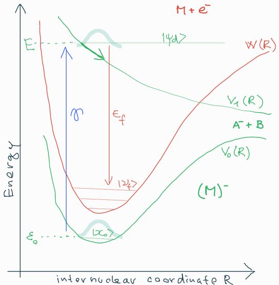
Figure 1: Schematic picture of the photodetachment process. All potentials, energies and states related to anion are drawn in green. The neutral molecule and the continuum-electron related quantities are in red and and the absorbed photon energy in blue.

II.1 Photodetachment in dipole approximation

The initial state $|\Psi_{0}\rangle\rangle$ for the photodetachment process is the assumed to be the ground state of the molecular anion $M^{-}$, which we consider in Born-Oppenheimer approximation. We used the double-ket notation to stress that the wavefunction is product of vibrational and electronic part $|\Psi_{0}\rangle\rangle=|\chi_{0}\rangle|\phi_{0}\rangle$, where $|\phi_{0}\rangle$ is the ground electronic state of the anion and the vibrational wavefunction $\chi_{0}(R)$ solves the usual Schrödinger equation

$$\left[T_{N}+V_{0}(R)\right]\chi_{0}(R)=\varepsilon_{0}\chi_{0}(R),$$ (5)

with the potential energy surface $V_{0}(R)$ depending on the nuclear geometry $R$, $T_{N}$ is the vibrational kinetic energy operator and $\varepsilon_{0}$ is energy of the initial vibrational state $|\chi_{0}\rangle$. The main goal of this paper is to evaluate the photodetachment amplitude

$$A=\langle\langle\Psi^{(-)}|D|\Psi_{0}\rangle\rangle=\langle\langle\Psi^{(-)}|D|\chi_{0}\rangle|\phi_{0}\rangle,$$ (6)

where $D$ is the electrical dipole operator and $|\Psi^{(-)}\rangle\rangle$ is the scattering wavefunction subjected to outgoing boundary condition fixing the final state vibrational state of the neutral molecule $|\nu_{f}\rangle$ and the outgoing electron state $|\epsilon_{f}\rangle$, with the energy subjected to conservation law

$$E=\varepsilon_{\gamma}+\varepsilon_{0}=\epsilon_{f}+E_{v_{f}},$$ (7)

with photon energy $\varepsilon_{\gamma}$ and vibrational energy of the final state of the molecule $E_{v_{f}}$.

We apply the discrete-state-in-continuum model and the projection-operator formalism to calculate the scattering wavefunction $|\Psi^{(-)}\rangle\rangle$. The starting point is the assumption of the existence of the diabatic basis in the Hilbert space of electrons with the fixed nuclei of the molecule, consisting of 1) at least two discrete states: already described ground state of the anion $|\phi_{0}\rangle$ and the excited metastable anion state $|\phi_{1}\rangle$ and 2) electron scatering continuum states. More discrete states can in principle be included but here we will limit the discussion to one bound and one discrete metastable state for simplicity. We can define the projector to the discrete state part of the electronic Hilbert space

$$\mathcal{Q}=\sum_{d}|\phi_{d}\rangle\langle\phi_{d}|.$$ (8)

and the complementary operator

$$\mathcal{P}=I-\mathcal{Q}$$ (9)

projecting on the background electron continuum $e^{-}+M$. The basis in this subspace can be chosen as solutions the background scattering problem

$$\mathcal{P}\mathcal{H}_{el}\mathcal{P}|\Phi_{0},\epsilon\mu\rangle=(W+\epsilon)|\Phi_{0},\epsilon\mu\rangle,$$ (10)

$W(R)$ is the potential energy surface of the neutral molecule, i. e. the energy of the ground electronic state $|\Phi_{0}\rangle$ of the neutral molecule and energy $\epsilon$ and quantum number $\mu$ identify the state of outgoing electron. Here we consider only the case that the neutral molecule has only one energetically accessible electronic state and we will suppress the symbol $\Phi_{0}$ in the notation. We also assume only one dominant partial wave and suppress also the symbol $\mu$. We thus ended with the basis states $|\epsilon\rangle$ which can be used to expand the projector on the continuum part of the Hilbert stat for each $R$

$$\mathcal{P}=\int|\epsilon\rangle\langle\epsilon|d\epsilon.$$ (11)

Now the fixed nuclei electronic hamiltonian $\mathcal{H}_{el}$ can be expandent in the basis

$$\langle\phi_{d}|\mathcal{H}_{el}|\phi_{d^{\prime}}\rangle = V_{d}(R)\delta_{dd^{\prime}},$$ (12)

$$\langle\phi_{d}|\mathcal{H}_{el}|\epsilon\rangle = V_{d\epsilon}(R),$$ (13)

$$\langle\epsilon|\mathcal{H}_{el}|\epsilon^{\prime}\rangle = [W_{0}(R)+\epsilon]\,\delta(\epsilon-\epsilon^{\prime}).$$ (14)

Note that we neglected the coupling $\langle\phi_{0}|\mathcal{H}_{el}|\phi_{1}\rangle\simeq 0$ of the two discrete states, which assumes well isolated bound state $|\phi_{0}\rangle$ with noncrossing potentials $V_{0}(R)$ and $V_{1}(R)$. This asumption can be released but we will avoid it in this work. We will also neglect the coupling of the bound state to the continuum by setting $V_{d\epsilon}(R)=0$ for $d=0$, but we include the nonzero amplitude $V_{1\epsilon}(R)$ which is responsible for the electron autodetachment from the state $|\phi_{1}\rangle$.

The wavefunction $|\Psi^{(-)}\rangle\rangle$ can also be expanded in this basis

$$|\Psi^{(-)}\rangle\rangle=|\psi_{d}\rangle|\phi_{d}\rangle+\int|\psi_{\epsilon}\rangle|\epsilon\rangle d\epsilon.$$ (15)

Note that due to the decoupling of the ground state $d=0$ we can consider only $d=1$ in this expansion. This wavefunction is subjected to the same outgoing boundary condition like in the case of electron-molecule scattering and the $R$-depenent expansion coefficients $\psi_{d}(R)\equiv|\psi_{d}\rangle$ and $\psi_{\epsilon}(R)\equiv|\psi_{\epsilon}\rangle$ can be found in the same wave like in that case [1, 2]. In the case of the vibrational excitation process the relevant T-matrix element reads (1)

$$T_{VE}=\langle\langle\Psi^{(-)}|V|\nu_{i}\rangle|\epsilon_{i}\rangle=\langle\psi_{d}|V_{d\epsilon_{i}}|\nu_{i}\rangle,$$ (16)

where $V=\mathcal{P}\mathcal{H}_{el}\mathcal{Q}+\mathcal{Q}\mathcal{H}_{el}\mathcal{P}$. Notice that the last expression uses only the $\psi_{d}$ component of the expansion (15). Now we will remind how this component is evaluated and we would also like to process the expression (6) for the photodetachment amplitude in analogy with the expression (16) for the vibrational excitation process. The components of the wavefunction (15) can be found by solving the Schrödinger equation with the hamiltonian $H=T_{N}+\mathcal{H}_{el}$ with the appropriate boundary condition

$$|\psi_{d}\rangle = 0+[E-H_{d}]^{-1}\int V_{d\epsilon}|\psi_{\epsilon}\rangle d\epsilon,$$ (17)

$$|\psi_{\epsilon}\rangle = |\nu_{f}\rangle\delta(\epsilon-\epsilon_{f})+[E-h_{0}-\epsilon]^{-1}V_{d\epsilon}|\psi_{d}\rangle.$$ (18)

By substituting the second of the equations into the first and slight rearangement we get

$$\left[E-H_{d}-F^{{\dagger}}(E-h_{0})\right]|\psi_{d}\rangle=V_{d\epsilon_{f}}|\nu_{f}\rangle,$$ (19)

where

$$H_{d} = T_{N}+V_{d}(R),$$ (20)

$$h_{0} = T_{N}+W(R),$$ (21)

$$F(\varepsilon) = \int_{0}^{\infty}V_{d\epsilon}(R)[\varepsilon-\epsilon+i\eta]^{-1}V_{d\epsilon}(R^{\prime})d\epsilon.$$ (22)

Note that the final vibrational states of the neutral molecule after photodetachment are solution of the Schrödinger equation

$$h_{0}|\nu_{f}\rangle=E_{\nu_{f}}|\nu_{f}\rangle.$$ (23)

The equation (19) is used in theory of VE process to solve the dynamics numerically. The formal solution can be written as

$$|\psi_{d}\rangle=\left[E-H_{d}-F^{{\dagger}}(E-h_{0})\right]^{-1}V_{d\epsilon_{f}}|\nu_{f}\rangle.$$ (24)

This leads to the well known simple expression for the vibrational excitation

$$T_{VE}=\langle\nu_{f}|V_{d\epsilon_{f}}\left[E-H_{d}-F(E-h_{0})\right]^{-1}V_{d\epsilon_{i}}|\nu_{i}\rangle.$$ (25)

For the photodetachment amplitude we also need the continuum component

$$|\psi_{\epsilon}\rangle = |\nu_{f}\rangle\delta(\epsilon-\epsilon_{f})+$$

$$+ \left[E-h_{0}-\epsilon\right]^{-1}V_{d\epsilon}\left[E-H_{d}-F^{{\dagger}}(E-h_{0})\right]^{-1}V_{d\epsilon_{f}}|\nu_{f}\rangle.$$

Before we substitute the solution (15) with the components (24) and (II.1) into photodetachment amplitude (6) we define the fixed-$R$ transition dipole moments to discrete state $|\phi_{1}\rangle$ and to background continuum $|\epsilon\rangle$

$$\mu_{d}(R) = \langle\phi_{1}|D|\phi_{0}\rangle,$$ (27)

$$\mu_{\epsilon}(R) = \langle\epsilon|D|\phi_{0}\rangle$$ (28)

so that

$$A=\langle\psi_{d}|\mu_{d}|\chi_{0}\rangle+\int\langle\psi_{\epsilon}|\mu_{\epsilon}|\chi_{0}\rangle d\epsilon$$ (29)

or after substituting for the wavefunction components

$$A = \langle\nu_{f}|V_{d\epsilon_{f}}\left[E-H_{d}-F\right]^{-1}\mu_{d}|\chi_{0}\rangle$$ (30)

$$+\langle\nu_{f}|\mu_{\epsilon_{f}}|\chi_{0}\rangle$$

$$+\langle\nu_{f}|V_{d\epsilon_{f}}\left[E-H_{d}-F\right]^{-1}M(E-h_{0})|\chi_{0}\rangle,$$

where in analogy with $F(\varepsilon)$ we have defined

$$M(\varepsilon)=\int_{0}^{\infty}V_{d\epsilon}(R)[\varepsilon-\epsilon+i\eta]^{-1}\mu_{\epsilon}(R^{\prime})d\epsilon.$$ (31)

This quantity can be interpreted as the transition amplitude through dipole transition to the continuum state $|\epsilon\rangle$ from which the electron is captured to the metastable anion state $|\phi_{1}\rangle$. The three terms in the photodetachment amplitude (30) have the following interpretation. The most simple is the second term $\langle\nu_{f}|\mu_{\epsilon_{f}}|\chi_{0}\rangle$ which gives the amplitude for the direct dipole photodetachment from the ground state to the bacground continuum

$$\gamma+M^{-}\to M(\nu_{f})+e^{-}.$$ (32)

The first term $\langle\nu_{f}|V_{d\epsilon_{f}}\left[E-H_{d}-F\right]^{-1}\mu_{d}|\chi_{0}\rangle$ is little bit more complicated as it describes the dipole transition to the discrete state $|\phi_{1}\rangle$ followed by an autodetachment to the neutral molecule and electron

$$\gamma+M^{-}\to\left(M^{-}\right)^{*}\to M(\nu_{f})+e^{-}.$$ (33)

The last term describes a three step process of dipole transition to intermediate continuum state from which electron is captured to $|\phi_{1}\rangle$ in second step followed by the third step of an autodetachment

$$\gamma+M^{-}\to e^{-}+M(\nu)\to\left(M^{-}\right)^{*}\to M(\nu_{f})+e^{-}.$$ (34)

It is difficult to estimate the relative importance of different mechanisms. We will discuss them on a simple model in the next section. Before that we notice that from the calculation point of view it is possible to merge the last to process into one expression and write the amplitude as the sum of direct and resonance processes

$$A=\langle\nu_{f}|\mu_{\epsilon_{f}}|\chi_{0}\rangle+\langle\nu_{f}|V_{d\epsilon_{f}}|\tilde{\psi}\rangle,$$ (35)

where the auxilary wavefunction $|\tilde{\psi}\rangle$ is obtained by solution of the equation

$$\left[E-T_{N}-V_{1}(R)-F\right]|\tilde{\psi}\rangle=\left[\mu_{d}+M(E)\right]|\chi_{0}\rangle.$$ (36)

II.2 Photodissociation of the anion

If the energy of the photon is small enough the process of the dissociative electron detachment

$$\gamma+M^{-}\to e^{-}+A+B,$$ (37)

where $A$ and $B$ are fragments of the neutral molecule $M\equiv AB$ is forbidden. The potentials sketched in Fig. 1 allow for the resonance dissociation of the anion

$$\gamma+M^{-}\to\left(M^{-}\right)^{*}\to A^{-}+B.$$ (38)

This process is contained in the amplitude of the wave-function $\tilde{\psi}(R)$ for $R\to\infty$ or it can be alternatively formulated using the solution with the outgoing boudary condition in the potential $V_{1}(R)$.

III Test model calculation

In this part we would like to test the proposed approach on a simple model of electron detachment from diatomic anion. The goal of this calculation is not quantitative description of the photodetachment cross sections for any specific molecule, but the parameters of the model are on the qualitative level inspired by lithium hydride anion [15, 16]. The model of the photodetachment as described above is determined by knowledge of the potential of the neutral molecule $W(R)$, the potential curve of the ground anion state $V_{0}(R)$, the excited anion state $V_{1}(R)$ (the discrete state), the discrete-state-continuum coupling function $V_{d\epsilon}(R)$ and the dipole moment transition elements $\mu_{d}(R)$ and $\mu_{\epsilon}(R)$. The discrete-state-continuum coupling function $V_{d\epsilon}(R)$ depends on the continuum cahnnel index (for example angular momentum), but in this simple model we assume that there is one dominant channel and neglect this dependence. Similarly the dipole transition moment is vector quantity, but we assume the fixed polarization with respect to molecular axis and treat is as a single number. These details would be important in comparison with specific experimental data, but they are not important in this qualitative discussion.

III.1 Qualitative model for diatomic molecule

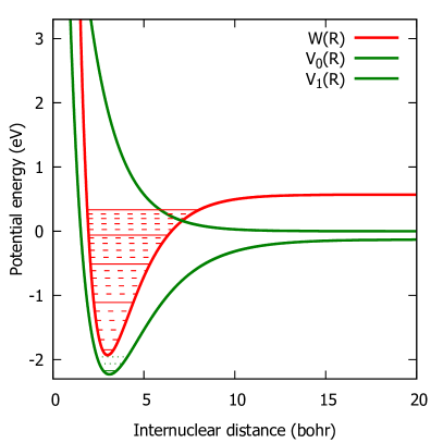
Figure 2: Potential energy curves in our model. The neutral molecule is in red and anion states in green. The vibrational levels are also shown (every fifth with solid line).

The potential energy curves $W(R)$ and $V_{0}(R)$ for the ground states of the neutral molecule and the anion can be calculated by well established mehtods of quantum chemistry. For LiH molecule high-level calculation is available [17]. We also calculated the potential energy curves (see Fig. 1 in [15]). Here, for the model calculation we use simply Morse potential, qulitatively similar to the LiH case. The exact form is as follows (numerical values are for the energies in eV and distances in Bohr)

$$W(R) = de^{-2a(R-R_{0})}-2de^{-a(R-R_{0})}+b,$$ (39)

$$V_{0}(R) = d_{0}e^{-2a_{0}*(R-R_{g})}-2d_{0}e^{-a_{0}*(R-R_{g})}+b_{0},$$ (40)

$$V_{1}(R) = d_{1}e^{-a_{1}*(R-R_{0})},$$ (41)

where $R_{0}=3.0$, $a=0.6$, $b=0.57$, $d=2.5$, $R_{g}=3.1$, $a_{0}=0.45$, $b_{0}=-0.13$, $d_{0}=2.1$, $a_{1}=0.6$ and $d_{1}=1.9$.

The discrete state potential $V_{1}(R)$ and its coupling to the continuum $V_{d\epsilon}(r)$ is often extracted by fitting the fixed-nuclei scattering phaseshifts. This is based on the solution of the fixed-R scattering problem with electronic hamiltonian parametrized as

$$\mathcal{H}_{el} = |\phi_{d}\rangle V_{d}\langle\phi_{d}|+\int|\epsilon\rangle\left\{W+\epsilon\right\}\langle\epsilon|d\epsilon$$ (42)

$$+\int\left\{|\phi_{d}\rangle V_{d\epsilon}\langle\epsilon|+|\epsilon\rangle V_{d\epsilon}\langle\phi_{d}|\right\}d\epsilon.$$

The solution of the scattering problem $|\Psi(E)\rangle$ at fixed molecular geometry $R$ can be expanded in the basis $|\phi_{d}\rangle$, $|\epsilon\rangle$ in similar way like (15)

$$|\Psi(E))\rangle=\psi_{d}|\phi_{d}\rangle+\int\psi_{\epsilon}|\epsilon\rangle d\epsilon.$$ (43)

Now $\psi_{d}$ and $\psi_{\epsilon}$ are numbers (dependent on $R$) not wavefunctions in vibrational space. It is easy to solve the scattering problem with hamiltonian (42) and to find the components

$$\psi_{d} = \left[E-V_{d}-F(E-W)\right]^{-1}V_{d\epsilon_{i}},$$ (44)

$$\psi_{\epsilon} = \delta(\epsilon-\epsilon_{i})+(E-\epsilon-W)^{-1}V_{d\epsilon}\psi_{d}.$$ (45)

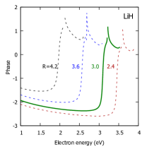
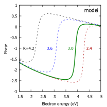
Figure 3: Fixed-nuclei scattering phaseshifts for few internuclear separations $R$ (labeled in the graphs). Figure in the left shows the results of R-matrix scattering calculations for LiH+e and the right panel is the result from our model.

The scattering phaseshift for the fixed-nuclei problem then reads[1]

$$\delta=-\arctan\left(\frac{\Gamma(\epsilon,R)/2}{\epsilon-V_{d}(R)-W(R)-\Delta(\epsilon,R)}\right),$$ (46)

with $\Delta$ and $\Gamma$ derived from the real and imaginary part of the fixed-nuclei version $F[E-W(R)]$

$$F(\varepsilon)=\Delta-{\textstyle\frac{i}{2}\Gamma}=\int V_{d\epsilon}(R)[\varepsilon-\epsilon+i\eta]^{-1}V_{d\epsilon}(R)d\epsilon.$$ (47)

of the nonlocal level-shift operator $F(E-h_{0})$ in (22). Notice that the operator-valued argument $E-h_{0}$ changed into electron energy $\epsilon=E-W(R)$ relative to the scattering threshold. The fitting of the formula (46) to ab initio scattering data for eigenpahses is usually used to obtain $V_{d}(R)$ and $V_{d\epsilon}$. Here we just choose the model functions by hand so that the resulting phaseshift (46) is in visual qualitative accordance with the data for LiH molecule [15] as demonstrated in Fig. 3.

The model function $V_{d}(R)=V_{1}(R)$ of Eq. (41) was choosen to obtain the data in the figure and the separable form of discrete-state-continuum coupling

$$V_{d\epsilon}(R) = g(R)f(e),$$ (48)

$$g(R) = \left[1+e^{0.75(R-6}\right]^{-1},$$ (49)

$$\gamma(\epsilon) \equiv 2\pi f(\epsilon)^{2}=A_{\gamma}[\epsilon/B_{\gamma}]^{\alpha}e^{-\epsilon/B_{\gamma}},$$ (50)

with constants $A_{\gamma}=1$eV, $B_{\gamma}=2$eV, $\alpha=0.2$ was used. This form is inspired by earlier studies of electron-molecule collisions [1, 2]. It is convenient that the integral transform (47) can be calculated analytically for this form.

The last ingredient of the model is the knowledge of the transition dipole moment $\mu_{d}$ to the discrete state and transition dipole moment function $\mu_{\epsilon}$ for each internuclear separation $R$. To do so we were again guided by the fixed-nuclei scattering calculation [15, 16] for LiH. The calculated moment function

$$|\mu|^{2}=|\langle\chi_{0}|D|\Psi(E))\rangle|^{2}$$

is shown in Fig. (4) in the left panel, but we have to keep in mind that the function $|\Psi(E)\rangle$ has both discrete-state and continuum components (44), (45). Substituting these in (43) we get relation to $\mu_{d}$ and $\mu_{\epsilon}$

$$\mu=\mu_{\epsilon}+\frac{\mu_{d}V_{d\epsilon}}{\epsilon-V_{d}-F(\epsilon)}+\frac{M(\epsilon)V_{d\epsilon}}{\epsilon-V_{d}-F(\epsilon)}.$$ (51)

Notice that this expression is fixed-nuclei version of (6) and the terms thus have similar interpretation: direct transition dipole to background continuum $\mu_{\epsilon}$ and the next two terms are the resonant contribution due to transition to the discrete state and subsequent autodetachment and term due to attachment to the discrete state from the background continuum.

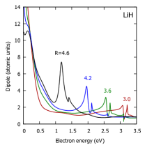
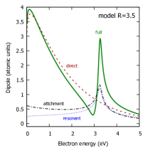
Figure 4: Transition dipole matrix element from the ground state anion to continuum for fixed-nuclei electronic problem. The internuclear separations $R$ are marked in the graphs. The left panel show the results of R-matrix calculation for LiH molecule, the right panel is calculated from our model, with contributions of three different terms marked separately.

We find that this function within our model (see Fig. 4 right panel) is in reasonable qualitative agreement with the calculation for LiH molecule. The three individual contributions are also shown in the figure but the full result is not direct sum of the individual contributions, because the complex phase has to be taken into account. The model functions producing the figure are

$$\mu_{d} = 0.1+0.1i,$$ (52)

$$2\pi\mu_{\epsilon}^{2} = A_{\mu}[\epsilon/B_{\mu}]^{\alpha}e^{-\epsilon/B_{\mu}},$$ (53)

with $A_{\mu}=150$a.u. and $B_{\mu}=0.8$eV. This form of the functions allows for calculation of the integral transform in the definition (31) of function $M(\epsilon)$ analytically in the same way as for function $F(\epsilon)$.

III.2 Notes on numerical treatment

To calculate the full photodetachment amplitude (30) we need to be able to apply the operator

$$|\Psi\rangle=\left[E-H_{d}-F\right]^{-1}|\Phi\rangle.$$

This is equivalent to solving the equation

$$\left[E-H_{d}-F\right]^{-1}|\Psi\rangle=|\Phi\rangle.$$

There are well developed techniques to perform this task in the treatment of the inelastic electron-molecule collision [1, 2] and we applied our numerical codes to perform this task. The operator $F(E-h_{0})$ needed there is evaluated by expansion into neutral molecule vibrational basis $h_{0}|\nu\rangle=E_{\nu}|\nu\rangle$ which converts it to evaluation of the fixed-nuclei quantity $F(\epsilon)$ calculated by the integral transform

$$F(E-h_{0})=\sum_{\nu}|\nu\rangle F(E-E_{\nu})\langle\nu|.$$ (54)

The same method can be used to calculate also the operator $M(E-h_{0})$.

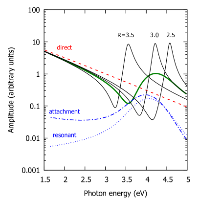
Figure 5: Dependence of the photodetachment amplitude on the photon energy (full green line). The results of full calculation is shown with contribution of different mechanisms also marked separately. Black lines show fixed nuclei amplitudes for three different values of $R$ for comparison.

III.3 Discussion of the results

The calculated results are shown in Fig. (5) and (6). In the first of the two figures the full amplitude $|A|^{2}$ for the final ground vibrational state of the neutral molecule formed after the detachment is plotted together with the three individual contributions. We see that resonance and attachment contributions have similar shape and are important only close to the resonance energy 4eV. We also show the fixed nuclei amplitude $|\mu|^{2}$ for three internuclear separations $R$. Observe that the full amplitude is given by smearing of the fixed nuclei amplitude over the initial vibrational wavefunction $\chi_{0}(R)$.

In Fig. (6) we show the amplitude for two energies $E=3$eV and $E=4$eV and for first 20 vibrational states of the final neutral molecule. For the energy 3eV, which is below the resonance, the amplitude decreases very fast with the vibrational quantum number. On the other hand the resonance energy $E=4$eV alows for creation of highly vibrationally excited energies which much larger probability. We also see that the background contribution continues to decay fast and the resonance and attachment contributions dominate for high vibrational quantum numbers.

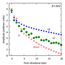
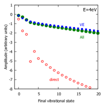
Figure 6: Amplitude for photodetachment to different final vibrational states of the neutral molecule. Two different photon energies are included $E=3eV$ (off-resonance, left) and $E=4eV$ (in resonance, right). Different symbols show full calculation (full circles) and direct photodetachment to background continuum (empty circles). Vibrational excitation cross sections of the neutral molecule by electron scattering are shown for comparison (squares).

IV Conclusions

We derived theory for calculation of the electron photodetachment from molecular anions in resonance condition using the discrete-state-in-continuum model in very similar way like in description of inelastic electron-molecule collisions. The techniques developed for the numerical treatment of the electron-molecule collisions can therefore be directly applied also for resonance photodetachment. We also expect that similar phenomena as the ones studied there (threshold peaks, Wigner cusps, boomerang oscillations) can have their analogs in photodetachment physics.