KD-FixMatch: Knowledge Distillation Siamese Neural Networks

Abstract

Semi-supervised learning (SSL) has become a crucial approach in deep learning as a way to address the challenge of limited labeled data. The success of deep neural networks heavily relies on the availability of large-scale high-quality labeled data. However, the process of data labeling is time-consuming and unscalable, leading to shortages in labeled data. SSL aims to tackle this problem by leveraging additional unlabeled data in the training process. One of the popular SSL algorithms, FixMatch [1], trains identical weight-sharing teacher and student networks simultaneously using a siamese neural network (SNN). However, it is prone to performance degradation when the pseudo labels are heavily noisy in the early training stage. We present KD-FixMatch, a novel SSL algorithm that addresses the limitations of FixMatch by incorporating knowledge distillation. The algorithm utilizes a combination of sequential and simultaneous training of SNNs to enhance performance and reduce performance degradation. Firstly, an outer SNN is trained using labeled and unlabeled data. After that, the network of the well-trained outer SNN generates pseudo labels for the unlabeled data, from which a subset of unlabeled data with trusted pseudo labels is then carefully created through high-confidence sampling and deep embedding clustering. Finally, an inner SNN is trained with the labeled data, the unlabeled data, and the subset of unlabeled data with trusted pseudo labels. Experiments on four public data sets demonstrate that KD-FixMatch outperforms FixMatch in all cases. Our results indicate that KD-FixMatch has a better training starting point that leads to improved model performance compared to FixMatch.

Index Terms—  semi-supervised learning, knowledge distillation, siamese neural networks, high-confidence sampling, deep embedding clustering

1 Introduction

Large-scale high-quality labeled data is the key to the tremendous success of supervised deep learning models in many fields. However, collecting labeled data remains a significant challenge, as the process of data labeling is time-consuming and resource-intensive. This is particularly evident in tasks such as detecting product image defects in e-commerce, where high-quality labeled data is essential for accurate predictions and customer satisfaction. The numbers of defective and non-defective images are sometimes extremely unbalanced and thus it is necessary to label a large number of randomly selected images in order to collect sufficient high-quality labeled images for supervised learning.

Recently, [1] came up with a widely used SSL algorithm called FixMatch, which trains an SNN with limited labeled and extra unlabeled data, and achieved significant improvement comparing to traditional supervised learning methods. However, despite the superiority and success of FixMatch, it has a noticeable disadvantage. It trains the teacher and the student in an SNN simultaneously and since the pseudo labels generated by the teacher in the early stage may not be correct, using them directly may introduce large amount of label noise. Therefore, we propose a modified FixMatch called KD-FixMatch, which trains an outer and an inner SNN sequentially. Our proposed method improves upon FixMatch because an outer SNN will be first trained with labeled and unlabeled data and thus the percentage of label noise in the pseudo labels generated by the network of the well-trained outer SNN would be lower than that of the teacher in FixMatch, especially in the early stage. Our main contributions are summarized as follows:

1. In KD-FixMatch, the outer SNN is first well-trained and its network serves as a teacher for the inner SNN. Thus, we have a better training starting point than direcly applying FixMatch algorithm to the inner SNN.

2. Unlike self-training [2, 3] or Noisy Student [4], where its neural network is re-trained multiple times when its pseudo labels are required to be updated, we only need to train each of the outer and inner SNN once.

3. KD-FixMatch outperforms FixMatch in our experiments although the time complexity of KD-FixMatch is more than two times that of FixMatch.

2 RELATION TO PRIOR WORK

SSL has gained significant attention in recent years as a method to overcome the challenge of limited labeled data. By incorporating large-scale unlabeled data, SSL has shown to enhance the performance of deep neural networks, as demonstrated in various studies [1, 4, 5, 6, 7].

2.1 Teacher-Student Sequential Training

Knowledge distillation [8] is a well-known model compression technique that transfers knowledge from a pre-trained, larger teacher model to a smaller student model. By using the teacher to generate pseudo labels for the unlabeled data, the student trained on both labeled data and pseudo-labeled data performs better than when trained solely on the limited labeled data [8].

Noisy Student [4] takes inspiration from knowledge distillation and uses a student model that is equal to or larger than the teacher model. This allows for the inclusion of noise-inducing techniques such as dropout, stochastic depth, and data augmentation in the student’s training, resulting in better generalization compared to the teacher [4]. In Noisy Student, once the student is found to be better than the teacher, the pseudo labels are updated by the current student, and a new student is re-initialized. This procedure is then repeated several times. However, this approach requires waiting for the teacher to be well-trained before generating highly confident pseudo labels for the student’s training.

2.2 Teacher-Student Simultaneous Training

Besides the aforementioned sequential methods, the simultaneous training method is also an alternative option [1, 9, 10]. We take FixMatch [1] as an example. The core neural network architecture for FixMatch is SNN which consists of two identical weight-sharing classifier networks, a teacher and a student. See Figure 1.

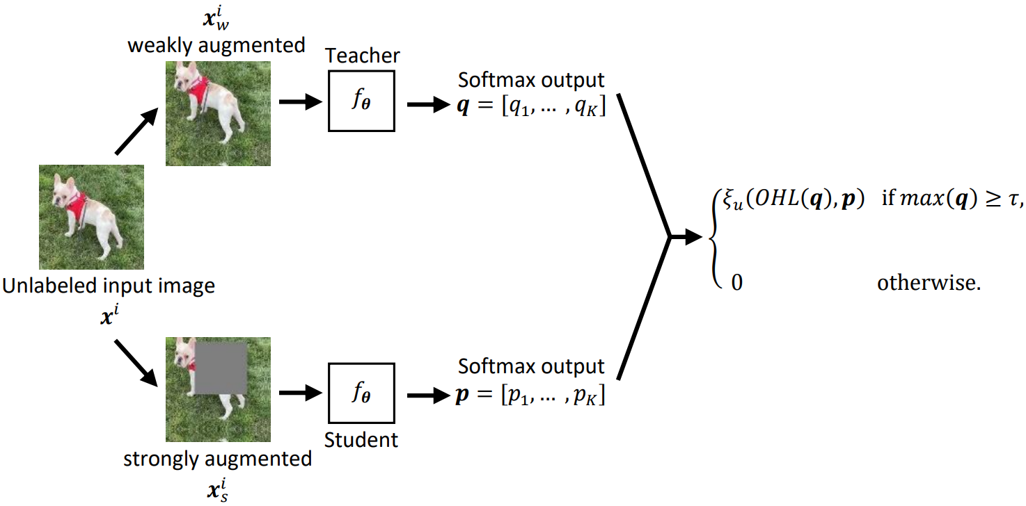
Fig. 1: An example of SNN for FixMatch.

Assume that $f_{\boldsymbol{\theta}}$ is a standard neural network with softmax output layer, $\boldsymbol{\theta}\in\Re^{n}$ is a long vector, $\ell$ is the number of training examples, $K$ is the number of the classes, and $n$ is the total number of the parameters of $f_{\boldsymbol{\theta}}$. We define the optimization problem for FixMatch to be

$$\min_{\boldsymbol{\theta}}\ f(\boldsymbol{\theta}),\text{where}\ f(\boldsymbol{\theta})=\frac{1}{2C}\boldsymbol{\theta}^{T}\boldsymbol{\theta}+\frac{1}{\ell}\sum_{i=1}^{\ell}\xi(\boldsymbol{\theta};{\boldsymbol{x}}^{i},{\boldsymbol{y}}^{i})$$ (1)

$C>0$ is the parameter to avoid overfitting by regularization, ${\boldsymbol{x}}^{i}$ is the $i$th input image, and ${\boldsymbol{y}}^{i}$ is the label vector of ${\boldsymbol{x}}^{i}$. In addition, if ${\boldsymbol{x}}^{i}$ belongs to the $s$th class, the label vector, ${\boldsymbol{y}}^{i}$, is $[\underbrace{0,\ldots,0}_{s-1},1,0,\ldots,0]^{T}\in\Re^{K}$. However, training examples for SSL consists of both a set of the labeled data, $S_{l}$, and a set of the unlabeled data, $S_{u}$. Label vectors for the unlabeled data are not available. Therefore, FixMatch uses teacher inside SNN to generate pseudo labels as label vectors for ${\boldsymbol{x}}^{i},i\in S_{u}$ and then the loss function, $\xi$, in (1) can be defined as follows:

$$\xi(\boldsymbol{\theta};{\boldsymbol{x}}^{i},{\boldsymbol{y}}^{i})=\begin{cases}\xi_{l}\left({\boldsymbol{y}}^{i},f_{\boldsymbol{\theta}}({\boldsymbol{x}}^{i}_{w})\right)&\text{if}\ \ i\in S_{l},\\ \lambda_{u}\xi_{u}(\hat{{\boldsymbol{y}}}^{i},f_{\boldsymbol{\theta}}({\boldsymbol{x}}^{i}_{s}))&\text{if}\ \ i\in S_{u},\end{cases}$$ (2)

where $\hat{{\boldsymbol{y}}}^{i}$ is the pseudo label vector of ${\boldsymbol{x}}^{i},i\in S_{u}$, $\lambda_{u}$ is a pre-defined parameter, ${\boldsymbol{x}}^{i}_{w}$ is the weakly augmented image of ${\boldsymbol{x}}^{i}$, ${\boldsymbol{x}}^{i}_{s}$ is the strongly augmented image of ${\boldsymbol{x}}^{i}$, $\xi_{l}$ is a loss function for the labeled data, and $\xi_{u}$ is a loss function for the unlabeled data.

In [1], $\xi_{l}$ in (2) is the standard cross-entropy (CE) function to measure the difference between $f_{\boldsymbol{\theta}}({\boldsymbol{x}}^{i}_{w})$ and its label vector ${\boldsymbol{y}}^{i}$. For $\xi_{u}$ in (2), when the input of $f_{\boldsymbol{\theta}}$ is ${\boldsymbol{x}}^{i}_{w}$, $f_{\boldsymbol{\theta}}$ is considered as the teacher and $f_{\boldsymbol{\theta}}({\boldsymbol{x}}^{i}_{w})$ is $\hat{{\boldsymbol{y}}}^{i}$ of ${\boldsymbol{x}}^{i}$. Conversely, $f_{\boldsymbol{\theta}}$ is considered as the student when the input of $f_{\boldsymbol{\theta}}$ is ${\boldsymbol{x}}^{i}_{s}$. However, in order to reduce label noise, we only choose the highly confident pseudo labels whose maximum value are greater than or equal to a pre-defined threshold $\tau>0$ and thus $\xi_{u}$ in (2) can be defined as follows:

$$\mathbb{1}(\max(\hat{{\boldsymbol{y}}}^{i})\geq\tau)\xi_{u}(\text{OHL}(\hat{{\boldsymbol{y}}}^{i}),f_{\boldsymbol{\theta}}({\boldsymbol{x}}^{i}_{s})),$$ (3)

where $\mathbb{1}$ is an indicator function and OHL is a function mapping a softmax pseudo label vector to its one-hot label vector. After the loss function, $\xi$, in (1) is prepared, back-propagation is applied to update the weights in $f_{\boldsymbol{\theta}}$ and thus both teacher and student are updated simultaneously by minimizing (1).

For the method where teacher and student are trained simultaneously, there is no need to wait for the teacher’s training procedure to complete before the student’s can begin. However, in the early stage, heavy label noise or insufficient correct pseudo labels generated by the immature teacher may affect the generalization ability of the student model.

3 Proposed Algorithm

We propose an algorithm called KD-FixMatch, which contains an outer SNN, $f^{\text{outer}}$, and an inner SNN, $f^{\text{inner}}$. The goal is not only to use teacher-student sequential training to fix label noise problem in the early stage, but also to incorporate teacher-student simultaneous training such as FixMatch.

3.1 Trusted Pseudo Label Selection

After the outer SNN is well-trained, it generates pseudo labels for the unlabeled data. Due to the imperfection of the outer SNN, we need to choose a subset of trusted pseudo labels to reduce label noise. Otherwise, it may affect inner SNN’s model performance.

Similar to (3), we first choose a pre-defined threshold, $\tau^{\text{select}}$, and choose the pseudo labels whose maximum value is greater than or equal to $\tau^{\text{select}}$. Then, we extract the latent representations of the unlabeled data which has passed the $\tau^{\text{select}}$ selection. We do a deep embedding clustering [11, 12] on the representations and choose the unlabeled data whose clustering results are consistent with their predicted class. Finally, the indices of the chosen unlabeled data form $T_{u}$.

3.2 Merging Conflict Pseudo Labels

From Section 3.1, $T_{u}$ is determined. However, our inner SNN also generates pseudo labels for the unlabeled data during its training process. Following (3), we choose the pseudo labels whose maximum value is greater than or equal to a pre-defined threshold, $\tau^{\text{inner}}>0$, to be inner SNN’s trusted pseudo labels. Therefore, conflicts may arise when both the outer and inner SNN provide their own trusted pseudo labels for the same image. Heuristic 1 is proposed to determine the pseudo label vector, $\hat{{\boldsymbol{y}}}^{i}$, in (3) for the unlabeled data which has conflict pusedo labels. The main idea is that the inner SNN intuitively has better generalization ability than the outer SNN since it has more reliable pseudo labels in the early stage.

if $\max\left(f^{\text{inner}}_{\boldsymbol{\theta}}({\boldsymbol{x}}^{i}_{w})\right)\geq\tau^{\text{inner}}$ then

       $\hat{{\boldsymbol{y}}}^{i}\leftarrow f^{\text{inner}}_{\boldsymbol{\theta}}({\boldsymbol{x}}^{i}_{w})$

else if $i\in T_{u}$ then

       $\hat{{\boldsymbol{y}}}^{i}\leftarrow{\boldsymbol{y}}^{i,\text{outer}}$

else

       $\hat{{\boldsymbol{y}}}^{i}\leftarrow{\boldsymbol{0}}$

end if

HEURISTIC 1 Merging Conflict Pseudo Labels

3.3 Robust Loss Functions

Label noise is one of the major problems for SSL since teacher model is not perfect. In other words, there exist noisy labels among the pseudo labels generated by the teacher. [7] mentioned that robust loss functions may be helpful in case of noisy pseudo labels. The widely used loss functions in robust learning is symmetric loss functions [13, 14] which has been proven to be robust to noisy labels. However, there are some constraints for symmetric loss functions.

Assume that $f$ is a standard neural network with softmax output layer. From [14], a loss function $\xi$ is called symmetric if it satisfies $\sum_{k=1}^{K}\xi(f({\boldsymbol{x}}),{\boldsymbol{e}}_{k})=M,\ \forall{\boldsymbol{x}}\in X,\ \forall f,$ where $K$ is the number of classes, $X$ is the feature space, $f$ is a function mapping an input ${\boldsymbol{x}}$ to a softmax output ${\boldsymbol{y}}$, $M$ is a constant value, and ${\boldsymbol{e}}_{k}=[\underbrace{0,\ldots,0}_{k-1},1,0,\ldots,0]^{T}\in\Re^{K}$.

Mean absolute error (MAE) [15], symmetric cross-entropy (SCE) [16], and normalized cross-entropy (NCE) [17] are examples of robust loss functions.

3.4 Knowledge Distillation Siamese Neural Networks

We initialize an inner SNN and then train it with not only the labeled and unlabeled data but also the unlabeled data with trusted pseudo labels, $({\boldsymbol{x}}^{i},\hat{{\boldsymbol{y}}}^{i}),i\in T_{u}$. For the inner SNN, the optimization problem and loss functions are the same as (1), (2), and (3) except that we substitute $f$, $C$, $\xi_{l}$, $\lambda_{u}$, $\xi_{u}$, and $\tau$ with $f^{\text{inner}}$, $C^{\text{inner}}$, $\xi^{\text{inner}}_{l}$, $\lambda^{\text{inner}}_{u}$, $\xi^{\text{inner}}_{u}$, and $\tau^{\text{inner}}$, respectively. A summary of our proposed algorithm is in Algorithm 2.

Given a labeled data, $S_{l}$, and an unlabeled data, $S_{u}$;

1: Initialize an outer SNN, $f^{\text{outer}}$, and train it with $S_{l}$ and $S_{u}$ by using back-propagation to solve (1);

2: Generate pseudo labels for $S_{u}$ using the well-trained $f^{\text{outer}}$;

3: Select a trusted index subset $T_{u}$ from $S_{u}$;

4: Choose CE or a robust loss function to be $\xi^{\text{inner}}_{u}$;

5: Initialize an inner SNN, $f^{\text{inner}}$, and train it with not only the labeled and unlabeled data but also the unlabeled data with trusted pseudo labels, $({\boldsymbol{x}}^{i},\hat{{\boldsymbol{y}}}^{i}),i\in T_{u}$;

6: Return the well-trained $f^{\text{inner}}$;

ALGORITHM 2 KD-FixMatch

4 Experiments

The main objective in this section is to compare our proposed algorithm with other methods. For a fair comparison, we implement all of the methods using Tensorflow 2.3.0. EfficientNet-B0 [18] pre-trained on ImageNet is chosen for all of the experiments and SNN-EB0 is an SNN which consists of two identical weight-sharing EfficientNet-B0. We compare the following five methods: (a) Baseline: EfficientNet-B0 is trained with only the labeled data by solving (1) with CE loss function; (b) FixMatch: SNN-EB0 is trained with the labeled and unlabeled data by solving (1) with (2) and (3) and both $\xi_{l}$ and $\xi_{u}$ are CE functions; (c) KD-FixMatch-CE: an outer and an inner SNN-EB0 are trained using Algorithm 2 with the labeled and unlabeled data and both $\xi_{l}$ and $\xi_{u}$ for outer and inner SNN-EB0 are CE functions; (d) KD-FixMatch-SCE-1.0-0.01: the same as KD-FixMatch-CE except that $\xi_{u}$ for inner SNN-EB0 is an SCE function with $\alpha=1.0$ and $\beta=0.01$; and (e) KD-FixMatch-SCE-1.0-0.1: the same as KD-FixMatch-CE except that $\xi_{u}$ for inner SNN-EB0 is an SCE function with $\alpha=1.0$ and $\beta=0.1$. For the labeled training data in all of our experiments, we follow the sampling strategy mentioned in [1] to choose an equal number of images from each class in order to avoid model bias.

For all the experiments, Adam [19] optimizer is used and the exponential decay rates for $1$st and $2$nd moment estimates are $0.9$ and $0.999$, respectively. Batch size is set to $128$. The initial learning rate is $7\mathrm{e}{-5}$ and the learning rate scheduler mentioned in Section $5.2$ of [18] is applied. We set $1/C$ in (1) to be $5\mathrm{e}{-4}$ except that $1\mathrm{e}{-3}$ for CIFAR100. For weak augmentation, we follow the method in Section 2.3 of [1]. For strong augmentation, we follow RandAugment implementation in [20]. Following [1], we set $\tau$ in (3) to be $0.95$ and $\lambda_{u}$ be $1$. Also, we set $\tau^{\text{select}}$ and $\tau^{\text{inner}}$ to be $0.80$ and $0.95$, respectively. For inference, we follow [1] to use the maintained exponential moving average of the trained parameters. The decay is set to be $0.9999$ and num_updates be $10$.

4.1 Experiments on Four Public Data Sets

In this subsection, we conduct our experiments on four public data sets: SVHN [21], CIFAR10/100 [22], and FOOD101 [23]. In order to mimic the practical use, we randomly split the training data from their official websites into original training data ($80\%$) and original validation data ($20\%$) for our experiments. The unlabeled data from the official websites is not used. Instead, we follow [1] to ignore the labels in the original training data and deem it as unlabeled data. All of these four data sets are publicly available and the summary is in Table 1.

	#class	#train	#validation	#test
CIFAR10	10	40,000	10,000	10,000
SVHN	10	58,606	14,651	26,032
CIFAR100	100	40,000	10,000	10,000
FOOD101	101	60,600	15,150	25,250

Table 1: Summary of four public data sets. #class is the number of classes, #train is the number of the train data, #validation is the number of the validation data, #test is the number of the test data.

From Table 2, we observe that: (a) FixMatch is better than Baseline for all the cases. This is as expected because, comparing to Baseline, FixMatch leverages an additional unlabeled data; (b) KD-FixMatch is better than FixMatch for all the cases. The reason is that KD-FixMatch has a better starting point than FixMatch; (c) Comparing to FixMatch, the more labeled data we use, the less improvements we have for KD-FixMatch. The possible reason is that when FixMatch has a large enough initial labeled data it has a good starting point to reach the result competitive to KD-FixMatch; and (d) KD-FixMatch-SCE has slightly better model performance than KD-FixMatch-CE in most of the cases even without grid search for the two parameters, $(\alpha,\beta)$. The possible reason is that the robust loss function, SCE, is applied.

	$400$ labels	$1,000$ labels	$2,000$ labels	$4,000$ labels
Baseline	$33.47\pm 4.62\%$	$44.18\pm 4.40\%$	$82.62\pm 1.90\%$	$93.37\pm 0.24\%$
FixMatch	$84.96\pm 0.75\%$	$91.85\pm 0.58\%$	$94.25\pm 0.47\%$	$95.69\pm 0.15\%$
KD-FixMatch-CE	$87.40\pm 0.53\%$	$92.92\pm 0.46\%$	$94.94\pm 0.25\%$	$96.18\pm 0.18\%$
KD-FixMatch-SCE-1.0-0.01	$87.33\pm 0.52\%$	$93.03\pm 0.54\%$	${\bf 95.04\pm 0.18\%}$	$96.33\pm 0.23\%$
KD-FixMatch-SCE-1.0-0.1	${\bf 87.55\pm 0.41\%}$	${\bf 93.19\pm 0.32\%}$	$95.00\pm 0.41\%$	${\bf 96.34\pm 0.13\%}$

(a) CIFAR10

	$400$ labels	$1,000$ labels	$2,000$ labels	$4,000$ labels
Baseline	$19.66\pm 23.56\%$	$30.23\pm 26.62\%$	$82.97\pm 0.98\%$	$87.06\pm 0.22\%$
FixMatch	$70.20\pm 2.11\%$	$83.40\pm 0.85\%$	$87.84\pm 1.90\%$	$89.91\pm 0.88\%$
KD-FixMatch-CE	$76.01\pm 1.37\%$	$84.50\pm 1.45\%$	${\bf 89.07\pm 0.90\%}$	$91.12\pm 0.38\%$
KD-FixMatch-SCE-1.0-0.01	$76.46\pm 1.65\%$	${\bf 84.52\pm 1.36\%}$	$89.06\pm 1.09\%$	${\bf 91.15\pm 0.75\%}$
KD-FixMatch-SCE-1.0-0.1	${\bf 76.50\pm 1.80\%}$	$84.40\pm 1.62\%$	$88.50\pm 1.08\%$	$91.11\pm 0.45\%$

(b) SVHN

	$1,000$ labels	$4,000$ labels	$10,000$ labels	$20,000$ labels
Baseline	$35.02\pm 30.12\%$	$71.92\pm 0.36\%$	$78.20\pm 0.34\%$	$81.97\pm 0.36\%$
FixMatch	$57.72\pm 1.02\%$	$73.73\pm 0.53\%$	$79.51\pm 0.87\%$	$82.74\pm 0.30\%$
KD-FixMatch-CE	${\bf 61.26\pm 0.96\%}$	$75.94\pm 0.65\%$	$81.05\pm 0.31\%$	$83.53\pm 0.52\%$
KD-FixMatch-SCE-1.0-0.01	$60.68\pm 0.96\%$	${\bf 76.01\pm 0.61\%}$	$80.75\pm 0.32\%$	$83.65\pm 0.36\%$
KD-FixMatch-SCE-1.0-0.1	$60.62\pm 0.96\%$	$75.57\pm 0.13\%$	${\bf 81.10\pm 0.15\%}$	${\bf 83.85\pm 0.28\%}$

(c) CIFAR100

	$1,000$ labels	$4,000$ labels	$10,000$ labels	$20,000$ labels
Baseline	$38.81\pm 0.38\%$	$59.87\pm 0.42\%$	$69.97\pm 0.19\%$	$75.62\pm 0.17\%$
FixMatch	$39.94\pm 0.42\%$	$63.26\pm 0.46\%$	$72.04\pm 0.33\%$	$77.38\pm 0.23\%$
KD-FixMatch-CE	$42.64\pm 0.96\%$	$65.60\pm 0.32\%$	$74.72\pm 0.39\%$	$79.33\pm 0.33\%$
KD-FixMatch-SCE-1.0-0.01	${\bf 43.18\pm 1.23\%}$	$65.94\pm 1.08\%$	$74.54\pm 0.30\%$	$79.29\pm 0.24\%$
KD-FixMatch-SCE-1.0-0.1	$41.73\pm 1.51\%$	${\bf 66.12\pm 1.10\%}$	${\bf 74.86\pm 0.33\%}$	${\bf 79.46\pm 0.09\%}$

(d) FOOD101

Table 2: Test accuracy for four public data sets. We run all the experiments five times using the same five random seeds and report the mean and standard deviation of the test accuracy. The best results in each column are represented in bold letters.

5 Conclusion

In this paper, we have proposed an SSL algorithm, KD-FixMatch, which is an improved version of FixMatch that utilizes knowledge distillation. Based on our experiments, KD-FixMatch outperforms FixMatch and Baseline on four public data sets. Interestingly, despite the absence of the parameter selection for SCE (robust loss function), the performance of KD-FixMatch-SCE is slightly better than KD-FixMatch-CE in most of the cases.

References

- [1] Kihyuk Sohn, David Berthelot, Nicholas Carlini, Zizhao Zhang, Han Zhang, Colin A Raffel, Ekin Dogus Cubuk, Alexey Kurakin, and Chun-Liang Li, “Fixmatch: Simplifying semi-supervised learning with consistency and confidence,” Advances in neural information processing systems, vol. 33, pp. 596–608, 2020.
- [2] David Yarowsky, “Unsupervised word sense disambiguation rivaling supervised methods,” in 33rd annual meeting of the association for computational linguistics, 1995, pp. 189–196.
- [3] David McClosky, Eugene Charniak, and Mark Johnson, “Effective self-training for parsing,” in Proceedings of the main conference on human language technology conference of the North American Chapter of the Association of Computational Linguistics. Citeseer, 2006, pp. 152–159.
- [4] Qizhe Xie, Minh-Thang Luong, Eduard Hovy, and Quoc V Le, “Self-training with noisy student improves imagenet classification,” in Proceedings of the IEEE/CVF conference on computer vision and pattern recognition, 2020, pp. 10687–10698.
- [5] David Berthelot, Nicholas Carlini, Ian Goodfellow, Nicolas Papernot, Avital Oliver, and Colin A Raffel, “Mixmatch: A holistic approach to semi-supervised learning,” Advances in Neural Information Processing Systems, vol. 32, 2019.
- [6] Bowen Zhang, Yidong Wang, Wenxin Hou, Hao Wu, Jindong Wang, Manabu Okumura, and Takahiro Shinozaki, “Flexmatch: Boosting semi-supervised learning with curriculum pseudo labeling,” Advances in Neural Information Processing Systems, vol. 34, pp. 18408–18419, 2021.
- [7] Wenhui Cui, Haleh Akrami, Anand A Joshi, and Richard M Leahy, “Semi-supervised learning using robust loss,” arXiv preprint arXiv:2203.01524, 2022.
- [8] Geoffrey Hinton, Oriol Vinyals, and Jeff Dean, “Distilling the knowledge in a neural network,” arXiv preprint arXiv:1503.02531, 2015.
- [9] Hieu Pham, Zihang Dai, Qizhe Xie, and Quoc V Le, “Meta pseudo labels,” in Proceedings of the IEEE/CVF Conference on Computer Vision and Pattern Recognition, 2021, pp. 11557–11568.
- [10] Antti Tarvainen and Harri Valpola, “Mean teachers are better role models: Weight-averaged consistency targets improve semi-supervised deep learning results,” Advances in neural information processing systems, vol. 30, 2017.
- [11] Junyuan Xie, Ross Girshick, and Ali Farhadi, “Unsupervised deep embedding for clustering analysis,” in International conference on machine learning. PMLR, 2016, pp. 478–487.
- [12] Xiangli Yang, Zixing Song, Irwin King, and Zenglin Xu, “A survey on deep semi-supervised learning,” IEEE Transactions on Knowledge and Data Engineering, 2022.
- [13] Naresh Manwani and PS Sastry, “Noise tolerance under risk minimization,” IEEE transactions on cybernetics, vol. 43, no. 3, pp. 1146–1151, 2013.
- [14] Aritra Ghosh, Himanshu Kumar, and PS Sastry, “Robust loss functions under label noise for deep neural networks,” in Proceedings of the AAAI conference on artificial intelligence, 2017, vol. 31.
- [15] CJ Willmott, SG Ackleson, RE Davis, JJ Feddema, KM Klink, DR Legates, J O’donnell, and CM Rowe, “Statistics for the evaluation of model performance,” J. Geophys. Res, vol. 90, no. C5, pp. 8995–9005, 1985.
- [16] Yisen Wang, Xingjun Ma, Zaiyi Chen, Yuan Luo, Jinfeng Yi, and James Bailey, “Symmetric cross entropy for robust learning with noisy labels,” in Proceedings of the IEEE/CVF International Conference on Computer Vision, 2019, pp. 322–330.
- [17] Xingjun Ma, Hanxun Huang, Yisen Wang, Simone Romano, Sarah Erfani, and James Bailey, “Normalized loss functions for deep learning with noisy labels,” in International Conference on Machine Learning. PMLR, 2020, pp. 6543–6553.
- [18] Mingxing Tan and Quoc Le, “Efficientnet: Rethinking model scaling for convolutional neural networks,” in International Conference on Machine Learning. PMLR, 2019, pp. 6105–6114.
- [19] Diederik P Kingma and Jimmy Ba, “Adam: A method for stochastic optimization,” arXiv preprint arXiv:1412.6980, 2014.
- [20] Ekin D Cubuk, Barret Zoph, Jonathon Shlens, and Quoc V Le, “Randaugment: Practical automated data augmentation with a reduced search space,” in Proceedings of the IEEE/CVF Conference on Computer Vision and Pattern Recognition Workshops, 2020, pp. 702–703.
- [21] Yuval Netzer, Tao Wang, Adam Coates, Alessandro Bissacco, Bo Wu, and Andrew Y Ng, “Reading digits in natural images with unsupervised feature learning,” 2011.
- [22] Alex Krizhevsky, Geoffrey Hinton, et al., “Learning multiple layers of features from tiny images,” 2009.
- [23] Lukas Bossard, Matthieu Guillaumin, and Luc Van Gool, “Food-101–mining discriminative components with random forests,” in European conference on computer vision. Springer, 2014, pp. 446–461.