Geodesics on Regular Constant Distance Surfaces

Abstract

Suppose that the surfaces $K_{0}$ and $K_{r}$ are the boundaries of two convex, complete, connected $C^{2}$ bodies in $\mathbb{R}^{3}$. Assume further that the (Euclidean) distance between any point $x$ in $K_{r}$ and $K_{0}$ is always $r$ ($r>0$). For $x$ in $K_{r}$, let $\Pi(x)$ denote the nearest point to $x$ in $K_{0}$. We show that the projection $\Pi$ preserves geodesics in these surfaces if and only if both surfaces are concentric spheres or co-axial round cylinders. This is optimal in the sense that the main step to establish this result is false for $C^{1,1}$ surfaces. Finally, we give a non-trivial example of a geodesic preserving projection of two $C^{2}$ non-constant distance surfaces. The question whether for any $C^{2}$ convex surface $S_{0}$, there is a surface $S$ whose projection to $S_{0}$ preserves geodesics is open.

2020 Mathematics Subject Classification: 52A15, 53A05.

1 Introduction

Suppose $\gamma(t)$ is a trajectory of an object in $\mathbb{R}^{3}$ outside a convex body. In this paper, $\Pi(\gamma(t))$ is called the projection of $\gamma(t)$. In many applications it is important to track the point $\Pi(\gamma(t))$ on the surface of the body nearest to the moving object. In [10], a method to compute and track the projection was considered. Instead, here we consider the question whether this projection can take geodesics to (reparametrized) geodesics.

Before describing the main result, we give some general background about this problem. A diffeomorphism $\phi:S_{1}\rightarrow S_{2}$ between (sub) manifolds is called a geodesic mapping if it carries geodesics to geodesics. We restrict our discussion to surfaces in $\mathbb{R}^{3}$. It is well-known that if $S_{1}$ has constant Gaussian curvature, then there is a geodesic mapping from $S_{1}$ to the plane. Vice versa, Beltrami’s theorem says that if $S_{1}$ admits a (local) geodesic mapping to the plane near every point in $S_{1}$, then $S_{1}$ has constant Gaussian curvature ([4], Section 4.6, exercises 12 and 13). There is a fairly large body of literature on geodesic mappings, [7, 8] and the references therein. Our own interest here is to find out whether projections from one surface to another can be geodesic mappings.

Our main result concerns projections to the convex set from a surface whose distance to the convex set is exactly $r$ (a constant). We call such a surface a surface of constant distance (the word ‘equidistant’ is already in use for a slightly different concept [11]). Very little has been written about sets of constant distance (but see [3, 2]). What we aim to show here is essentially a rigidity result in $\mathbb{R}^{3}$: a constant distance surface whose projection takes geodesics to geodesics must be a sphere or a cylinder. We proceed with the details.

We imagine a $C^{2}$ convex body in $\mathbb{R}^{3}$ whose boundary we denote by $K_{0}$. Let $p$ be any point in the surface. By applying an isometry, we may assume that $p$ is located at the origin of $\mathbb{R}^{3}$ and that the tangent plane to $K_{0}$ at $p$ is given by $z=0$. Thus the coordinate patch near the origin can be written as

$$K_{0}(x_{1},x_{2})=\left(x_{1},x_{2},-\frac{1}{2}(a_{1}x_{1}^{2}+a_{2}x_{2}^{2})-h(x_{1},x_{2})\right)\,,$$ (1.1)

where the $a_{i}$ are the principal curvatures and $h$ is twice continuously differentiable with $h(0,0)$ is zero and the same holds for all first and second derivatives. By convexity, the principal curvatures $a_{i}$ are non-negative.

Because of the smoothness and the convexity, we can smoothly coordinatize the space $\Omega$ surrounding the convex body by using these coordinate patches as follows [10]:

$$S(x_{1},x_{2},r)=K_{0}(x_{1},x_{2})+r\hat{n}(x_{1},x_{2})\,.$$ (1.2)

where $\hat{n}$ is the unit normal to $K_{0}$. These 3-dimensional coordinate patches form a differentiable atlas of $\Omega$. Denote by $\Pi:\Omega\rightarrow K_{0}$ the orthogonal ‘projection’ from $\Omega$ onto $K_{0}$, defined as follows [10]: $\gamma:=\Pi(z)$ is the unique point on $K_{0}$ nearest to $z\in\Omega$. Clearly, the inverse of $\Pi$ at a point $\gamma$ of $K_{0}$ consists of a ray normal to $K_{0}$ at $\gamma$.

$$\Pi^{-1}(\gamma)=\cup_{r>0}\{\gamma+r\hat{n}(\gamma)\}\,,$$

where $\hat{n}$ is the unit normal at $\gamma$ pointing outwards.

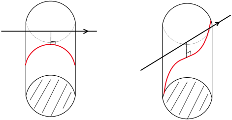
Figure 1.1: Left, the projection (red) of straight line orthogonal to the axis of symmetry of a solid cylinder. Right, the projection of a line at an arbitrary angle with the axis of symmetry of the cylinder. The former is a geodesic, the latter clearly not.

The simple example of Figure 1.1 shows that the projection of a straight line in $\mathbb{R}^{3}$ does not usually result in a geodesic in $K_{0}$. The question arises when is it that geodesics do project to geodesics? In this paper, any non-singular reparametrization (i.e. with non-zero, possibly variable, speed) of a unit speed geodesic will also be called a geodesic.

Definition 1.1

i) Given two closed $C^{2}$ surfaces $S_{1}$ and $S_{2}$ in $\mathbb{R}^{3}$. The projection $\Pi:S_{1}\rightarrow S_{2}$ is defined as follows. For $x\in S_{1}$,

$$\Pi(x):=\{y\in S_{2}\,:\,y\textrm{ minimizes the Euclidean distance }d(x,y)\}\,.$$

ii) Two surfaces are called regular constant distance surfaces if the Euclidean distance from any point $x$ in $S_{1}$ to $S_{2}$ equals $r$ (fixed), and the nearest point on $S_{2}$ is always unique.

It is a curious fact that in general $\Pi:S_{1}\rightarrow S_{2}$ and $\Pi^{\prime}:S_{2}\rightarrow S_{1}$ are not inverses of one another. However, if the $S_{i}$ are at least $C^{1}$ and regular constant distance, then $\Pi$ and $\Pi^{\prime}$ are inverses. This is the content of Proposition 2.1. In the remainder of this paper, we deal with this case (except where mentioned otherwise).

Let $K_{r}$ denote the surface that has distance $r$ to $K_{0}$, or

$$K_{r}:=\{S(x_{1},x_{2},r)\,:\,r>0\textrm{ fixed}\}\,.$$

We are interested in determining when the projection $\Pi:K_{r}\rightarrow K_{0}$ between these surfaces have the property that they send geodesics to (reparametrizations of) geodesics. We call this property preservation of geodesics and $\Pi$ a geodesic mapping. The proof of the following result takes up most of this paper.

Theorem 1.2

Let $K_{0}$ be $C^{2}$ surface patch given by (1.1) with $a_{1}\geq 0$ and $a_{2}\geq 0$ and fix $r>0$. Then the projection $\Pi:K_{r}\rightarrow K_{0}$ does not preserve geodesics, unless (in that patch) (i) the Gaussian curvature is zero (i.e. $a_{1}a_{2}=0$) or (ii) the patch consists of umbilic points (i.e. $a_{1}=a_{2}$)

A moment’s reflection, will tell us that in $\mathbb{R}^{3}$, projections between concentric spheres or between co-axial round cylinders do preserve geodesics. The interesting question is, are there any others? Here is a (to the author) surprising corollary of Theorem 1.2.

Corollary 1.3

Let $K_{0}$ and $K_{r}$ be regular constant distance, complete, convex, connected, $C^{2}$ surfaces in $\mathbb{R}^{3}$ at a distance $r>0$. The projection from $K_{r}$ to $K_{0}$ preserves geodesics if and only if both are either spheres or (infinite) round cylinders.

Remark. In this context, a (generalized) cylinder $C$ is a set of points such that for every point $p\in C$ there is a unique line $\ell(p)$ in $C$ and any two such lines are either the same or parallel. A ‘perfect’ or ‘round’ cylinder is a cylinder that rotationally symmetric around its axis. In particular, its principal curvatures are constant.

Remark. In view of Proposition 2.1, $\Pi:K_{r}\rightarrow K_{0}$ and $\Pi^{\prime}:K_{0}\rightarrow K_{r}$ are inverses. So $\Pi$ preserves geodesics if and only if $\Pi^{\prime}$ preserves geodesics.

Proof of Corollary 1.3. It is clear that if $K_{0}$ and $K_{r}$ both are either spheres or (infinite) round cylinders, then the geodesics are preserved.

Vice versa, if the projection preserves geodesics, then by Theorem 1.2, every $C^{2}$ surface patch is either a piece of a sphere or piece of a cylinder. The two cannot occur in the same $C^{2}$ patch, because at any ‘intermediate’ point, (i) or (ii) in that theorem will be violated, and then geodesics will not be preserved. Thus all of $K_{0}$ must satisfy either (i) or (ii).

It is well-known that a $C^{2}$ complete surface whose principal curvatures are the identical (or umbilic surface) must be a part of a sphere ([4], Section 3.2). Similarly ([4], section 5.8), a complete surface with Gaussian curvature zero, must be a generalized cylinder. Finally, Proposition 4.1 implies that if $K_{0}$ and $K_{r}$ are cylinders and the projection preserves geodesics, then they must be round cylinders.  

Remark. Interestingly, this corollary is clearly false in $\mathbb{R}^{2}$. For instance, if $K_{0}$ is an ellipse in $\mathbb{R}^{2}$ and $K_{r}$ a circle that contains it, the projection $K_{r}\rightarrow K_{0}$ is surjective. On the other hand, in dimension 4 or higher, nothing appears to be known.

We furthermore prove that Corollary 1.3 is optimal in the sense that if we drop $C^{2}$ in favor of $C^{1,1}$, that is: once continuously differentiable with a Lipschitz derivatives, then the result does not hold.

Theorem 1.4

There exist regular constant distance, complete, convex, $C^{1,1}$ surfaces $K_{0}$ and $K_{r}$ in $\mathbb{R}^{3}$ with the property that (wherever the surfaces are $C^{2}$) either (i) $a_{1}a_{2}=0$ or (ii) $a_{1}=a_{2}$ holds, but the projection from $K_{0}$ to $K_{r}$ does not preserve geodesics.

Proof. The result follows directly from Proposition 5.1.  

Remark. In [1] (see also [10]), a related, but more complicated, counter-example was constructed which carries over to cylinders in $\mathbb{R}^{3}$. It says that here is a convex $C^{1,1}$ cylinder such that the projection $\Pi$ onto this cylinder does not have a derivative.

Finally, we are interested in the question whether, given the boundary $S_{0}$ of a convex body, there is any surface $S$ outside it, whose projection onto $S_{0}$ preserves geodesics. For cylinders in $\mathbb{R}^{3}$, the answer is affirmative, as we show in Section 6. In fact, in that case, the space outside $S_{0}$ can be foliated by surfaces $S_{k}$, $k\geq 0$ so that each projection $\Pi_{k}:S_{k}\rightarrow S_{0}$ preserves geodesics. However, as we will show, these surfaces $S_{k}$ generally are not convex.

Remark. For general $C^{2}$ convex bodies, even in $\mathbb{R}^{3}$, it is unknown at the time of this writing whether the space outside them can be foliated by surfaces $S_{k}$ so that each projection $\Pi_{k}:S_{k}\rightarrow S_{0}$ preserves geodesics.

2 Preliminaries

We first prove that the projections between two regular constant distant surfaces (see Definition 1.1) are inverses of one another. Then we discuss the strategy to prove Theorem 1.2.

Proposition 2.1

Let $S_{1}$ and $S_{2}$ be $C^{1}$ surfaces in $\mathbb{R}^{3}$ such that the Euclidean distance from any point $x$ in $S_{1}$ to $S_{2}$ equals $r$ (fixed), and the nearest point on $S_{2}$ is always unique. Then the projections $\Pi:S_{1}\rightarrow S_{2}$ and $\Pi^{\prime}:S_{2}\rightarrow S_{1}$ are inverses of one another.

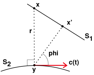
Figure 2.1: This figure illustrates that $\Pi:S_{1}\rightarrow S_{2}$ and $\Pi^{\prime}:S_{2}\rightarrow S_{1}$ are not generally inverses of one another. Traveling from $y$ along $S_{2}$ in the direction of $c(t)$ will (initially) decrease the distance to $x^{\prime}$.

Proof. Consider $\Pi:S_{1}\rightarrow S_{2}$ and $\Pi^{\prime}:S_{2}\rightarrow S_{1}$ and suppose $\Pi(x)=y$ (see Figure 2.1). Suppose there is $x^{\prime}$ in $S_{2}$ not equal to $x$ such that $x^{\prime}\in\Pi^{\prime}(y)$. Denote the Euclidean distance by $d(x,y)$. Now

$$x^{\prime}\in\Pi^{\prime}(y)\quad \Longrightarrow \quad d(y,x^{\prime})\leq d(y,x)=r$$

$$d(x^{\prime},S_{2})=r\quad \Longrightarrow \quad d(x^{\prime},y)\geq r$$

So $d(y,x^{\prime})=r$.

Consider the plane $P$ through $x$, $x^{\prime}$, and $y$, and parametrize $S_{2}$ by the arclength $t$ and let the geodesic $c(t)$ be the tangent to $S_{2}(t)$ as drawn in Figure 2.1. Then, by differentiability of $S_{2}$,

$$\lim_{t\searrow 0^{+}}\frac{d(S_{2}(t),x^{\prime})-d(S_{2}(0),x^{\prime})}{t}=\lim_{t\searrow 0^{+}}\frac{d(c(t),x^{\prime})-d(c(0),x^{\prime})}{t}=-\cos\phi\,.$$

The last equality is a special case of Theorem 4.3 in [5]. Thus for some positive $t$, $d(S_{2}(t),x^{\prime})<r$, contradicting the assumption that $d(x^{\prime},S_{2})=r$.  

To prove Theorem 1.2, we pick a family $\Gamma$ of geodesics in the patch given by (1.1) as follows. A geodesic $\gamma(t)$ in $\Gamma$ is determined by initial condition $\gamma(0)=(0,x_{2}(0),x_{3}(0))$, where $x_{2}(0)$ is not zero but small and $\dot{x}_{1}(0)>0$ is of order unity, while $x_{3}(0)$ is determined by the fact that $\gamma$ is a curve in the surface $K_{0}$ (see Figure 2.2).

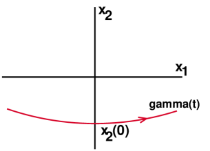
Figure 2.2: A view of a geodesic $\gamma$ in $K_{0}$ from ‘above’ (i.e. $x_{3}>0$). At $t=0$, $\gamma$ passes through the point $(0,x_{2}(0))$ with velocity $(\dot{x}_{1}(0),0)$.

Since we are interested not in geodesics per se, but in geodesics modulo (non-singular) reparametrization, we establish a simple characterization of geodesics in $\Gamma$ that does not depend on the parametrization (Lemma 3.1). We then consider the projection $\Pi:K_{0}\rightarrow K_{r}$, with $r>0$, which maps $\gamma$ to a curve $\gamma_{r}$ in $K_{r}$. And finally, we prove that $\gamma_{r}$ is not a (reparametrization of a) geodesic by showing that it fails the criterion just mentioned. To do this, we will need to determine the terms of the leading order of magnitude in a fairly involved expression. We will employ the standard ‘big-oh’ and ‘small-oh’ notation as follows. We consider curves such as the ones in Figure 2.2, and evaluate certain quantities as these curves cross the $x_{1}=0$ axis. Thus using $x$ as shorthand for $(x_{1},x_{2})$:

$$f(x_{1},x_{2}) = Ok\quad\textrm{means}\quad\limsup_{|x|\rightarrow 0}\frac{|f(x)|}{|x|^{k}}<\infty\,,$$

$$\textrm{and }\quad\quad f(x_{1},x_{2}) = ok\quad\textrm{means}\quad\lim_{|x|\rightarrow 0}\frac{|f(x)|}{|x|^{k}}=0\,.$$

It will be convenient to have a more compact notation. Hence the following definition.

Definition 2.2

We define $z_{i}:=a_{i}x_{i}+\partial_{i}h(x)$, where $x(t)=(x_{1}(t),x_{2}(t))$ is the projection to the $x_{1}$-$x_{2}$ plane of the geodesic $\gamma(t)$ in Figure 2.2.

We compute the leading orders at $t=0$ of $z_{i}$, $\dot{z}_{i}$, and $\ddot{z}_{i}$.

$$\dot{z}_{i}=a_{i}\dot{x}_{i}+d_{t}\partial_{i}h\quad\;\;{\rm and}\;\;\quad\ddot{z}_{i}=a_{i}\ddot{x}_{i}+d_{t}^{2}\partial_{i}h\,.$$

We know that $h=o2$ and so $\partial_{i}h=o1$. Furthermore, at $t=0$, $x_{1}=0$, and $x_{2}=O1$. Thus

$$z_{1}=\partial_{1}h\quad\;\;{\rm and}\;\;\quad z_{2}=a_{2}x_{2}+o1\,.$$ (2.1)

Each of these is $O1$ or less. Now,

$$d_{t}\partial_{i}h=\partial_{1}\partial_{i}h\;\dot{x}_{1}+\partial_{2}\partial_{i}h\;\dot{x}_{2}\,.$$

Along the geodesic in the patch, $\dot{x}_{1}$ is order unity (or $O1$), and even though $\dot{x}_{2}$ may be small, we see that $d_{t}\partial_{2}h=o0$. In fact, we are only interested in evaluating these quantities at $t=0$ at which point we have $\dot{x}_{2}=\ddot{x}_{2}=0$. Putting this together results at $t=0$ in

$$\dot{z}_{1}=a_{1}\dot{x}_{i}+o0\quad\;\;{\rm and}\;\;\quad\dot{z}_{2}=\partial_{1}\partial_{2}h\;\dot{x}_{1}\,,$$ (2.2)

and so $\dot{z}_{2}=o0$. The next derivative, $\ddot{z}_{i}$, is a little trickier. The reason is that $d_{t}^{2}\partial_{2}h$ cannot be bounded by some order. It may be large, or, depending on $h$, it may be small. To ensure we have the leading terms of $\ddot{z}_{i}$, we have to include both terms and the expression does not simplify. Setting $t=0$, we will see that $\ddot{x}_{1}=O1$ and we know that $\ddot{x}_{1}=0$. So at $t=0$,

$$\ddot{z}_{1}=a_{1}\ddot{x}_{i}+d_{t}^{2}\partial_{2}h\quad\;\;{\rm and}\;\;\quad\ddot{z}_{2}=\partial_{1}\partial_{2}h\;\dot{x}_{1}\,.$$ (2.3)

3 Proof of Theorem 1.2

To distinguish the standard inner product in $\mathbb{R}^{3}$ from a 2-tuple, we indicate the former by a dot: $x\cdot y$. Also, to avoid cluttering the formulas with the repetitive occurrence of the argument “(0)”, we will not write it, except when its omission might lead to misunderstandings.

Lemma 3.1

Suppose the family of curves $\gamma(t)=(x_{1}(t),x_{2}(t),-\frac{1}{2}[a_{1}x_{1}(t)^{2}+a_{2}x_{2}(t)^{2}]-h)$ in $K_{0}$ are (a reparametrization of) geodesics with $x_{1}=0$, $\dot{x}_{1}>0$, $x_{2}\neq 0$, and $\dot{x}_{2}=0$. Then at $t=0$

$$\lim_{x_{2}\rightarrow 0}\,\dfrac{\ddot{x}_{2}}{\dot{x}_{1}^{2}x_{2}}=-a_{1}a_{2}\,.$$

Furthermore, this characterization is independent of the (smooth) parametrization of $\gamma$.

Proof. Set $e_{i}:=\partial_{i}K_{0}$, where $K_{0}$ is given by (1.1). The metric tensor $g_{ij}=e_{i}\cdot e_{j}$ and its inverse are given by (see Definition 2.2)

$$g=\begin{pmatrix}1+z_{1}^{2}&z_{1}z_{2}\\ z_{1}z_{2}&1+z_{2}^{2}\end{pmatrix}\quad\;\;{\rm and}\;\;\quad g^{-1}=\Delta^{-1}\begin{pmatrix}1+z_{2}^{2}&-z_{1}z_{2}\\ -z_{1}z_{2}&1+z_{1}^{2}\end{pmatrix}\,,$$

where $\Delta$ is the determinant of $g$. The coefficients of $g^{-1}$ are denoted by $g^{ij}$. The Christoffel symbols of the second kind are now given by

$$\Gamma^{k}_{ij}:=\partial_{i}e_{j}\cdot\sum_{n}g^{kn}e_{n}\,.$$

We have that

$$\partial_{i}e_{j}=(0,0,-\partial_{i}z_{j})\,.$$

So we only need the 3rd component of $\sum_{n}g^{kn}e_{n}$. A straightforward computation gives that these are $-\Delta^{-1}z_{k}$. This yields

$$\Gamma^{k}_{ij}=\Delta^{-1}z_{k}\;\,\partial_{i}z_{j}\,.$$

Employing the rules for order calculation, one checks that this gives an $O1$ term only if $i=j$, namely $a_{i}x_{i}$. Everything else gives at best $o1$ terms. So $\Gamma^{k}_{ii}=a_{k}a_{i}x_{k}+o1$, and $\Gamma^{k}_{ij}=o1$ if $i\neq j$. The geodesic equations are

$$\ddot{x}_{k}+\sum_{i,j}\Gamma^{k}_{ij}\dot{x}_{i}\,\dot{x}_{j}=0\,.$$

So in our case, the equation for $\ddot{x}_{2}$ is

$$\begin{matrix}\ddot{x}_{2}+(a_{1}a_{2}x_{2}+o1)\,\dot{x}_{1}^{2}+(o1)\dot{x}_{1}\dot{x}_{2}+(a_{2}^{2}x_{2}+o1)\,\dot{x}_{2}^{2}=0\,.\end{matrix}$$

Setting $\dot{x}_{2}=0$, proves the first part of the lemma.

To prove that this is invariant under the parametrization $t\rightarrow s(t)$, define $c(t)=\gamma\circ s$. Set $s(0)=0$. Using $\dot{x}_{2}(0)=0$ again, it is trivial to show that at $t=0$

$$\frac{d_{t}^{2}(x_{2}(s))}{(d_{t}x(s))^{2}\,x_{2}(s)}=\dfrac{\ddot{x}_{2}}{\dot{x}_{1}^{2}x_{2}}\,,$$

where we use $d_{t}$ for $\tfrac{d}{dt}$.  

Lemma 3.2

Given the surface $K_{0}$ of (1.1), then the constant distance surface $K_{r}$ can be parametrized as follows

$$K_{r}(u_{1},u_{2})=\left(u_{1},u_{2},r-\frac{1}{2}(a_{1r}u_{1}^{2}+a_{2r}u_{2}^{2})+o2\right)\,,$$

where

$$a_{ir}=\dfrac{a_{i}}{1+ra_{i}}\,.$$

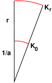
Figure 3.1: The radius of curvature in the $x$-direction of $K_{0}$ at the origin equals $1/a$. The orthogonal projection to $K_{r}$ then gives a radius of curvature of $r+1/a$. The principal curvature is the reciprocal of this.

Proof. Fix $r>0$. The inverse projection $\Pi_{r}^{-1}:K_{0}\rightarrow K_{r}$ is well-defined, and given by

$$K_{r}(x_{1},x_{2}):=\Pi_{r}^{-1}(K_{0}(x_{1},x_{2}))=K_{0}(x_{1},x_{2})+r\hat{n}(x_{1},x_{2})\,.$$ (3.1)

We’ll call $K_{0}$, somewhat informally, the ‘downstairs’ surface and $K_{r}$ is ‘upstairs’. We compute, using Definition 2.2

$$\hat{n}(x_{1},x_{2})=\frac{(z_{1},z_{2},1)}{\sqrt{1+z_{1}^{2}+z_{2}^{2}}}\,.$$ (3.2)

So

$$K_{r}(x_{1},x_{2}) = \left(x_{1}+\frac{rz_{1}}{V},x_{2}+\frac{rz_{2}}{V},-\frac{1}{2}(a_{1}x^{2}+a_{1}x_{2}^{2})-h(x_{1},x_{2})+\frac{r}{V}\right)\,,$$

$$\;\;{\rm where}\;\;V = \sqrt{1+z_{1}^{2}+z_{2}^{2}}$$

There are no mixed quadratic terms of the form $x_{1}x_{2}$ in the expansion of $K_{r}(x_{1},x_{2})$. So if we rewrite this as $K_{r}(u_{1},u_{2})=(u_{1},u_{2},r+u_{3}(u_{1},u_{2}))$, then the $u_{1}$- and $u_{2}$-axes of $K_{r}$ are the axes of principal curvature at $(u_{1},u_{2})=(0,0)$. All we need to do to complete the proof, is a computation of the curvature in the $x_{1}$-$r$ plane to get $a_{1r}$. This is done in Figure 3.1 by employing osculating circles. The computation is the same in the $x_{2}$-$r$ plane.  

Part of the difficulty here is that it is pretty clear that if $K_{0}$ does not have constant curvature along a geodesic $\gamma(t)$, then the curve traced in $K_{r}$ by projecting $\gamma$ will certainly not be a constant speed curve, let alone a constant speed geodesic. It is thus a priori clear that the projected curve will not satisfy the geodesic equations. What we wish to establish, however, is whether it can be reparametrized as a geodesic. We use Lemma 3.1 that the images $\gamma_{r}$ ($r>0$) under the projection are not geodesics.

Lemma 3.3

The geodesic $\gamma$ depicted in Figure 2.2 with $\gamma(0)=(0,x_{2})$ and $\dot{\gamma}(0)=(\dot{x}_{1},0)$ projects to a curve

$$\gamma_{r}(t)=(u_{1}(t),u_{2}(t),u_{3}(t))$$

in $K_{r}$ ($r>0$), where at $t=0$, we have

$$\dot{u}_{1} = (1+ra_{1})\dot{x}_{1}+o0$$

$$u_{2} = (1+ra_{2})x_{2}+o1$$

$$\ddot{u}_{2} = -(1+ra_{1}+ra_{2})a_{1}a_{2}\dot{x}_{1}^{2}x_{2}+rd_{t}^{2}\partial_{2}h+o1\,.$$

Proof. We trace a possibly reparametrized geodesic $\gamma(t)$ in $K_{0}$ satisfying Lemma 3.1, and determine the curvature of its projection $\gamma_{r}$ ‘upstairs’ in $K_{r}$. Note that $\gamma_{r}(t)$ is given by $\gamma(t)+r\hat{n}(x_{1}(t),x_{2}(t))$. The unit-normal $\hat{n}$ is given in (3.2). We use the rules of evaluating the orders given in Section 2.

The $x_{1}$ and $x_{2}$ coordinates of $\gamma_{r}$ will be called $u_{1}$ and $u_{2}$ and, noting that $z_{i}=O1$ (Section 2), we get

$$\begin{matrix}u_{1}=x_{1}+rz_{1}(1-\frac{1}{2}z_{1}^{2}-\frac{1}{2}z_{2}^{2}+O4)\\[8.5359pt] u_{2}=x_{2}+rz_{2}(1-\frac{1}{2}z_{1}^{2}-\frac{1}{2}z_{2}^{2}+O4)\,.\end{matrix}$$

Referring to (2.1), this gives for $u_{2}$ the following:

$$u_{2}=(1+ra_{2})x_{2}+o1\,.$$ (3.3)

Now, differentiate the $u_{i}$ with respect to time.

$$\begin{matrix}\dot{u}_{1}=\dot{x}_{1}+r\dot{z}_{1}-r\dot{z}_{1}(\frac{1}{2}z_{1}^{2}+\frac{1}{2}z_{2}^{2}+O4)-r\dot{z}_{1}(z_{1}\dot{z}_{1}+z_{2}\dot{z}_{2}+O3)\\[8.5359pt] \dot{u}_{2}=\dot{x}_{2}+r\dot{z}_{2}-r\dot{z}_{2}(\frac{1}{2}z_{1}^{2}+\frac{1}{2}z_{2}^{2}+O4)-r\dot{z}_{2}(z_{1}\dot{z}_{1}+z_{2}\dot{z}_{2}+O3)\,.\end{matrix}$$

Use (2.2), to see that the leading term appearing in $\dot{u}_{1}$ is $\dot{x}_{1}$ (which is $O0$), and thus

$$\dot{u}_{1}=(1+ra_{1})\dot{x}_{1}+o0\,.$$ (3.4)

We need to differentiate $\dot{u}_{2}$ one more time with respect to time.

$$\ddot{u}_{2} = \underbrace{\ddot{x}_{2}+\ddot{z}_{2}}_{A}-\underbrace{r\ddot{z}_{2}\;O2}_{B}-\underbrace{2r\dot{z}_{2}(z_{1}\dot{z}_{1}+z_{2}\dot{z}_{2}+O3)}_{C}-\underbrace{rz_{2}(\dot{z}_{1}^{2}+z_{1}\ddot{z}_{1}+\dot{z}_{2}^{2}+z_{2}\ddot{z}_{2}+O2)}_{D}\,.$$

To analyze this, we denote the four terms A through D, and look at each individually. In A, $\ddot{z}_{2}$ can be evaluated via (2.3) and $\ddot{x}_{2}$ can be eliminated via Lemma 3.1. This gives $-(1+ra_{2})a_{1}a_{2}\dot{x}_{1}^{2}x_{2}+rd_{t}^{2}\partial_{2}h$ for the term marked A. Clearly, B is negligible compared to A. In C, $\dot{z}_{2}=o0$ as noted before, and the term in parentheses is $O1$. So all together this term is $o1$ and therefore negligible compared to A. Finally, in C, we use (2.1) to establish that $-r\dot{z}_{1}^{2}z_{2}$ is $O1$ and, by (2.1), all other terms are smaller. This last expression can be simplified using (2.1) and (2.2) to $-ra_{1}^{2}a_{2}\dot{x}_{1}^{2}x_{2}+o1$. Collecting terms and adding the relations (3.3) and (3.4) yields the lemma.  

Proof of Theorem 1.2. On the one hand, if the projected curve $\gamma_{r}$ is also a geodesic, then it itself must satisfy Lemma 3.1 with the curvatures given by Lemma 3.2. So

$$\ddot{u}_{2}=-\frac{a_{1}a_{2}}{(1+ra_{1})(1+ra_{2})}\dot{u}_{1}^{2}u_{2}\,.$$

Eliminating $\dot{u}_{1}$ and $u_{2}$ in favor of $\dot{x}_{1}$ and $x_{2}$ via Lemma 3.3 gives

$$\ddot{u}_{2}=-(1+ra_{1})a_{1}a_{2}\dot{x}_{1}^{2}x_{2}+o1\,.$$

On the other hand, another equation for $\ddot{u}_{2}$ is given by Lemma 3.3. If we equate the two expressions, we obtain

$$-(1+ra_{1})a_{1}a_{2}\dot{x}_{1}^{2}x_{2}+o1=-(1+ra_{1}+ra_{2})a_{1}a_{2}\dot{x}_{1}^{2}x_{2}+rd_{t}^{2}\partial_{2}h+o1\,.$$

Upon simplification, this gives

$$-ra_{1}a_{2}^{2}\dot{x}_{1}^{2}x_{2}+rd_{t}^{2}\partial_{2}h=o1\,.$$ (3.5)

This equation has two possible solutions. The first is if the left hand is $o1$ and so $a_{1}a_{2}=0$ and $d_{t}^{2}\partial_{2}h$ is $o1$. From the rules about manipulating the order symbols in Section 2, it follows that then $h=o4$. The other possibility is if $a_{1}a_{2}>0$ and so $d_{t}^{2}\partial_{2}h=a_{1}a_{2}^{2}\dot{x}_{1}^{2}x_{2}+o1$. This happens if and only if $h=\tfrac{1}{4}a_{1}a_{2}^{2}x_{1}^{2}x_{2}^{2}+g$ and $d_{t}^{2}\partial_{2}g=o1$. So $h=\tfrac{1}{4}a_{1}a_{2}^{2}x_{1}^{2}x_{2}^{2}+o4$.

Now consider the geodesic $\eta$ which is just $\gamma$ rotated by $\pi/2$. Then, by the same reasoning, if the projection $\eta_{r}$ in $K_{r}$ is a geodesic, we must have that $h=\tfrac{1}{4}a_{1}^{2}a_{2}x_{1}^{2}x_{2}^{2}+o4$. Since both must hold, we get $\tfrac{1}{4}a_{1}a_{2}^{2}x_{1}^{2}x_{2}^{2}=\tfrac{1}{4}a_{1}^{2}a_{2}x_{1}^{2}x_{2}^{2}$ or $a_{1}=a_{2}$.  

Remark. The two types of solutions of (3.5) in this proof do indeed occur. For if $K_{0}$ is a plane or a cylinder with radius $1/a$, we get

$$K(x_{1},x_{2})=\sqrt{a^{-2}-x_{1}^{2}}-a^{-1}=-\tfrac{1}{2}ax_{1}^{2}-\tfrac{1}{8}a^{3}x_{1}^{4}+O6\,.$$

In this case, the Gaussian curvature is zero and $h=o4$. On the other hand, for a sphere of radius $1/a$, we have

$$K(x_{1},x_{2})=\sqrt{a^{-2}-x_{1}^{2}-x_{2}^{2}}-a^{-1}=-\frac{1}{2}(ax_{1}^{2}+ax_{2}^{2})-\frac{1}{8}(a^{3}x_{1}^{4}+2a^{3}x_{1}^{2}x_{2}^{2}+a^{3}x_{2}^{4})+O6\,.$$

Here, the principal curvatures are equal and $d_{t}^{2}\partial_{2}h=a^{3}\dot{x}_{1}^{2}x_{2}+o1$.

4 Cylinders Must Be Round

Now let $K_{0}$ be a convex, but not necessarily round, cylinder, invariant under translations along the $x_{3}$-axis. Consider “polar” coordinates $(\rho,x_{3},r)$ in $\mathbb{R}^{3}$ where $\rho$ is the arclength along the simple, closed curve in the $x_{1}$-$x_{2}$ plane that defines $K_{0}$ as illustrated in Figure 4.1.

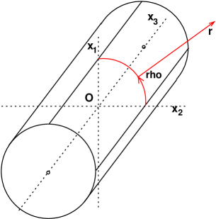
Figure 4.1: “Polar” coordinates in $\mathbb{R}^{3}$.

Proposition 4.1

With the above assumptions, the projection $\Pi:K_{0}\rightarrow K_{r}$ preserves geodesics if and only if the non-zero principal curvature of $K_{0}$ is constant.

Proof. Since the Gaussian curvature is zero, the map from the cylinder to the plane, given by $K_{0}(\rho,x_{3})\rightarrow(\rho,x_{3})$ is a bijective isometry and so maps geodesics to geodesics. A geodesic $\gamma$ in $K_{0}$ is (a) parallel to the $x_{3}$-axis, or (b) a circle in the $x_{1}$-$x_{2}$ plane, or (c) a curve $\gamma(x_{3})=(\rho(x_{3}),x_{3})$. Since $\gamma$ is a geodesic, $\rho(x_{3})$ is affine and has a constant derivative $\frac{d\rho}{dx_{3}}$. Assume $\gamma$ is a geodesic of type (c).

Now consider the projection $\gamma_{r}$ of $\gamma$ onto $K_{r}$. As with $K_{0}$, we parametrize $K_{r}$ by the arclength $\rho_{r}$ of the defining curve and $x_{3}$. It is clear that $\gamma_{r}$ is a curve $x_{3}\rightarrow\rho_{r}(x_{3})$. Again, if $\gamma_{r}$ is a geodesic, then $\frac{d\rho_{r}}{dx_{3}}$ is constant. Denote the non-zero principal curvature of $K_{0}$ by $a(\rho)$. A reasoning similar to that of Lemma 3.2 gives that arclengths $\rho_{r}$ and $\rho$ travelled along each geodesic relate as

$$d\rho_{r}=\frac{1/a(\rho)+r}{1/a(\rho)}\,\,d\rho=(1+a(\rho)r)\,\,d\rho\,.$$

Since the $x_{3}$ coordinates of $\gamma(t)$ and its projection $\gamma_{r}(t)$ are the same, we get

$$\frac{d\rho_{r}}{dx_{3}}=(1+a(\rho)r)\,\,\frac{d\rho}{dx_{3}}\,.$$ (4.1)

Thus $\frac{d\rho_{r}}{dx_{3}}$ is constant if and only if $a(\rho)$ is constant.  

5 A $C^{1,1}$ Counter-example

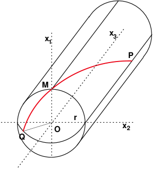
Figure 5.1: A straight cylinder of radius $r$ topped off by a hemisphere of radius $r$. This surface is $C^{2}$, except on the circle where the cylinder and the hemisphere meet. Here $\partial^{2}/\partial z^{2}$ has a discontinuity. Since the first derivative changes gradually, this surface is $C^{1,1}$.

We consider the round cylinder ‘topped off’ by a hemisphere both of radius $r$, which gives a $C^{1,1}$ surface (see Figure 5.1). Denote this surface by $S_{r}$. It is easy to convince oneself that $S_{1}$ and $S_{r}$ ($r>1$) are regular, constant distance surfaces. Clearly, at every point (except where $C^{2}$ does not hold) either (i) $a_{1}a_{2}=0$ or (ii) $a_{1}=a_{2}$.

Proposition 5.1

Let $S_{1}$, $S_{r}$, and $\Pi:S_{1}\rightarrow S_{r}$ be given as above. Let $\gamma_{1}$ be the shortest geodesic connecting $P_{1}=(0,1,\pi/2)$ and $Q_{1}=(0,-1/\sqrt{2},-1/\sqrt{2})$. The projection of $\gamma_{1}$ by $\Pi$ to $\gamma_{r}$ (connecting $P_{r}$ to $Q_{r}$ in $S_{r}$ ($r>1$)) is not a local geodesic near the point $M_{r}$ where $\gamma_{r}$ intersects the boundary of the cylinder (see Figure5.1).

Proof. The geodesic $\gamma$ connects $P_{1}$ to $Q_{1}$, but we do not know where it crosses over from the cylinder to sphere. So let us call that point $M_{1}(\theta)$. We have

$$P_{1}=(0,1,\pi/2)\;,\quad M_{1}(\theta)=(\sin\theta,\cos\theta,0)\;,\quad Q_{1}=\left(0,\tfrac{-1}{\sqrt{2}},\tfrac{-1}{\sqrt{2}}\right)\,.$$

It is easy to see that then the projection $\gamma_{r}$ of $\gamma$ connects $P_{r}$ to $Q_{r}$ via $M_{r}(\theta)$ (the same $\theta$), where

$$P_{r}=(0,r,\pi/2)\;,\quad M_{r}(\theta)=(r\sin\theta,r\cos\theta,0)\;,\quad Q_{r}=\left(0,\tfrac{-r}{\sqrt{2}},\tfrac{-r}{\sqrt{2}}\right)\,.$$ (5.1)

The projection of $\gamma_{r}$ consists of two pieces that live on $C^{2}$ surfaces with either curvature zero (the cylinder) or the sphere, and so each of these two pieces is a geodesic in $S_{r}$.

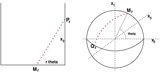
Figure 5.2: The two geodesic pieces of $\gamma_{r}$ in $S_{r}$. To the left, the piece in the flattened out cylinder. To the right the piece that lies in the hemisphere.

The first piece connects $P_{r}$ to $M_{r}$, see the left of Figure 5.2. In the flattened out cylinder, it is the hypotenuse of the triangle with sides $\pi/2$ and $r\theta$ and thus has length $\sqrt{\pi^{2}/4+r^{2}\theta^{2}}$. The second piece lives in the sphere. Its length is $r$ times the angle $\alpha$ between $M_{r}$ and $Q_{r}$. The cosine of $\alpha$ is given by the dot product of the unit vectors parallel to $M_{r}$ and $Q_{r}$, which gives $-\cos\theta/\sqrt{2}$. Thus the length of the second piece equals $r\arccos\left(\tfrac{-\cos\theta}{\sqrt{2}}\right)$. Therefore, the length of the projected curve $\gamma_{r}$ is given by

$$\ell_{\theta}(\gamma_{r})=\sqrt{\frac{\pi^{2}}{4}+r^{2}\theta^{2}}+r\arccos\left(\frac{-\cos\theta}{\sqrt{2}}\right)\,.$$

We need to minimize this over $\theta\in[0.\pi]$. It is an elementary calculus exercise to see that this is minimized at $\theta$ satisfying $\frac{\theta}{\sin\theta}=\frac{\pi/2}{r}$. We know that $\gamma$ is minimizing in $S_{1}$. Therefore if we substitute $r=1$, we get $\theta=\pi/2$. That same calculation for $r>1$ implies then that $\gamma_{r}$ (where $r>1$) is not globally minimizing in $S_{r}$.

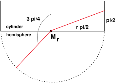
Figure 5.3: The tangent space $TS_{r}$ at $M_{r}$. The red curve corresponds to the lift of $\gamma_{r}$. The branch to the left of the base point $M_{r}$ travels to $Q_{r}$ and the branch to the right travels $P_{r}$ (see (5.1)).

Figure 5.3 is a slightly impressionistic image of the tangent space $TS_{r}$ at $M_{r}$. The slope of $\gamma_{r}$ restricted to the lower half plane that projects to the hemisphere equals 1. However the slope restricted the upper half plane which can be identified with the rolled out cylinder, the slope equals $1/r$. Thus $\gamma_{r}$ is not locally minimizing at $M_{r}$.  

6 There are Other Projections that Preserve Geodesics

In this Section, we find a beautiful example of a family of projections $\Pi_{k}:S_{k}\rightarrow S_{0}$ such that the surfaces $\left\{S_{k}\right\}_{k\geq 0}$ foliate the space surrounding the boundary $S_{0}$ of a convex body in $\mathbb{R}^{3}$. It is not known whether this is possible for all such surfaces $S_{0}$. Our construction is based on Section 4 and works for (convex) cylinders.

Consider a general, not necessarily round, convex, cylinder $S_{0}$. It consists of parametrized closed curve $c(t)$ and lines though that curve, orthogonal to it, as sketched in Figure 4.1. We can define a $S$ outside $S_{0}$ by first defining a new curve in $\mathbb{R}^{2}$:

$$C(t)=c(t)+r(t)\hat{n}(t)\,.$$

Here $\hat{n}(t)$ is the unit normal to $c(t)$ and $r(t)$ is a non-negative distance. Let us denote the curvature of $c(t)$ by $a(t)$. According to (4.1), the projection $\Pi:S\rightarrow S_{0}$ between the corresponding cylinders preserves geodesics if

$$r(t)=\frac{k}{a(t)}\,,$$

where $k$ is a positive constant. The cylinder $S_{k}$, $k\geq 0$ is given by the lines through $C_{k}$ orthogonal to plane of $C_{k}$. Thus the projection $\Pi_{k}:S_{k}\rightarrow S_{0}$ preserves geodesics. Notice that we have to be careful here, because now the back and forth projections are not inverses of one another anymore (see Proposition 2.1).

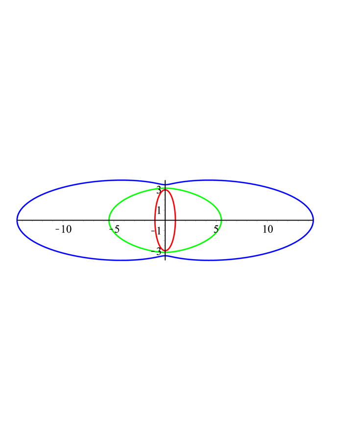
Figure 6.1: the cylinders orthogonal to the plane of the figure through the blue and the green curves, have projections to the cylinder orthogonal to the red ellipse that preserve geodesics.

We take as an example the ellipse given by

$$c(t):=(\alpha\cos(t),\beta\sin(t))\quad\;\;{\rm and}\;\;\quad C_{k}(t)=c(t)+\frac{k}{a(t)}\;\hat{n}(t)\,,$$

where $k$ is a non-negative constant. Standard calculations give $C(t)$ explicitly as

$$C_{k}(t)=\left(\left(\alpha+\frac{k}{\alpha}(\alpha^{2}\sin(t)^{2}+\beta^{2}\cos(t)^{2})\right)\cos(t),\left(\beta+\frac{k}{\beta}(\alpha^{2}\sin(t)^{2}+\beta^{2}\cos(t)^{2})\right)\sin(t)\right)\,.$$

We used MAPLE in Figure 6.1, to draw the ellipse $c(t)=(\cos(t),3\sin(t))$ in red, $C_{k}(t)$ for $k=0.5$ in green, and for $k=1.5$ in blue. Note that these remarkable curves lose convexity for large enough $k$. We leave it to the reader to establish that for large $k$, the projection $\Pi_{k}^{\prime}:S_{0}\rightarrow S_{k}$ is not single-valued and therefore does not preserve geodesics.

References

[1]
S. S. Akmal, M. N. Nam, J. J. P. Veerman, On a Convex Set with Nondifferentiable Metric
Projection, Optimization Letters, Vol 9, Issue 6, 1039-1052, 2015.
[2]
A. Blokh, M. Misiurewicz, L. Oversteegen, Sets of Constant Distance from a Compact Set in
2-Manifolds with a Geodesic Metric, Proceedings of the American Mathematical Society,
137, 733-743, 2009.
[3]
M. Brown, Sets of Constant Distance from a Planar Set, Michigan Math. J. 19, 321-323,
1972.
[4]
M. P. do Carmo (1976), Differentiable Geometry of Curves and Surfaces, Prentice-Hall, London.
[5]
L. S. Fox, P. Oberly, J. J. P. Veerman, One-Sided Derivative of Distance to a Compact Set,
Rocky Mountain Journal of Mathematics 51 (2), 491-508, 2021.
[6]
P. Michel, The ESA Hera Mission: Detailed Characterization of the DART Impact Outcome and of
the Binary Asteroid (65803) Didymos, The Planetary Science Journal, 3: 160, 2022 (July).
[7]
J. Mikes, Geodesic Mappings of Affine-Connected and Riemannian Spaces, J. Math. Sciences, 78 (3), 1996,
311-333.
[8]
J. Mikes, V. E. Berezovski, E. Stepanova, and H. Chudá, Geodesic Mappings and their Generalizations,
J. Math. Sciences, 217 (5), 2016, 608-623.
[9]
S.P. Naidu e. a., Radar observations and a physical model of binary near-Earth asteroid
65803 Didymos, target of the DART mission, Icarus, 348, 133777, 2020.
[10]
J. J. P. Veerman (2020), Navigating Around Convex Sets, The American Mathematical Monthly,
127:6, 504-517,
[11]
J. B. Wilker, Equidistant Sets and their Properties, Proceedings of the American
Mathematical Society, 47 (2): 446-452, 1975.