Robust Physics-based Deep MRI Reconstruction Via Diffusion Purification

Abstract

Deep learning (DL) techniques have been extensively employed in magnetic resonance imaging (MRI) reconstruction, delivering notable performance enhancements over traditional non-DL methods. Nonetheless, recent studies have identified vulnerabilities in these models during testing, namely, their susceptibility to (i) worst-case measurement perturbations and to (ii) variations in training/testing settings like acceleration factors and k-space sampling locations. This paper addresses the robustness challenges by leveraging diffusion models. In particular, we present a robustification strategy that improves the resilience of DL-based MRI reconstruction methods by utilizing pretrained diffusion models as noise purifiers. In contrast to conventional robustification methods for DL-based MRI reconstruction, such as adversarial training (AT), our proposed approach eliminates the need to tackle a minimax optimization problem. It only necessitates fine-tuning on purified examples. Our experimental results highlight the efficacy of our approach in mitigating the aforementioned instabilities when compared to leading robustification approaches for deep MRI reconstruction, including AT and randomized smoothing.

1 Introduction

Magnetic resonance imaging (MRI) is a widely used clinical tool for visualizing anatomical and physiological structures. However, its data acquisition is typically slow due to sequential processes. To overcome this limitation, various techniques[1, 2, 3] have emerged, enabling precise image reconstruction from limited, rapidly acquired data.

Deep learning (DL) serves as a tool for tackling large-scale inverse problems and addressing challenges in image reconstruction [4, 5, 3, 6]. This study is centered on the application of DL in the context of MRI reconstruction. Among various DL techniques, established networks designed for denoising images or sensor data are essential components. The widely adopted U-Net architecture [7, 8, 9] has been utilized to remove artifacts in MRI data resulting from undersampling. There has been particular interest in hybrid approaches that combine neural networks with imaging physics, including forward models. A particular notable example is MoDL (Model-based reconstruction using Deep Learned priors) [3], which employs an iterative approach to address the regularized inverse problem in MRI reconstruction.

Recent research highlights potential vulnerabilities in DL-based MRI reconstruction models, particularly susceptibility to small additive disturbances [10, 11, 12, 13]. Variations in acquisition settings further pose challenges, leading to reduced performance and potential diagnostic inaccuracies.

Various techniques have been developed to enhance the robustness of DL-based MRI reconstruction tasks [13, 14]. One noteworthy approach, adversarial training (AT) [15], originally devised to enhance the robustness of image classifiers [15, 16, 17, 18], involves solving a computationally intensive minimax optimization problem that incorporates generating adversarial examples. Another method, randomized smoothing (RS) [18], also initially designed for image classifiers, smoothens network outputs when handling inputs perturbed by random noise. Nevertheless, both AT and RS have demonstrated limitations in their performance when encountering previously unseen disturbances or dealing with larger perturbation bounds.

Within the domain of image classification, a recent study conducted by Nie et al. [19] has introduced a robustification strategy that effectively eliminates additive worst-case perturbations, harnessing the power of diffusion models (DMs) [20, 21, 22]. Drawing inspiration from this methodology, we investigate the application of a similar approach to enhance the resilience of the DL-based inverse problem formulation of MRI reconstruction. Our approach centers on the application of pre-trained diffusion models. More precisely, this purification process entails a gradual introduction of noise, followed by the refinement of the noise through the utilization of the pre-trained DM. Our approach yields substantial improvements in robustness, effectively countering not only worst-case additive perturbations but also addressing instabilities stemming from differences in settings between training and testing for the forward operator. In what follows, we outline the contributions of this article.

1.1 Contributions

• We introduce a robustification framework designed to enhance the resilience of state-of-the-art (SOTA) DL-based MRI reconstructors against additive perturbations and other instabilities. This is accomplished through purification via pre-trained DMs.

• We prove that the perturbed and clean images’ distributions (and conditional distributions) get closer to each other as the time moves forward in the diffusion stage.

• We present a novel approach to select a process-switching time step - a critical parameter within the DM-based purification method. This eliminates the necessity of treating it as a hyper-parameter.

• We use fine-tuning to improve performance, which, unlike SOTA robustification method AT, neither requires solving a minimax problem nor involves generating adversarial examples.

• In our experimental results, we demonstrate the effectiveness of our proposed approach by assessing it against standard evaluation metrics. Our results affirm that our strategy significantly surpasses the performance of AT and RS. Furthermore, we illustrate that after being trained on the knee fastMRI dataset, the purification process using DMs extends its benefits to other MRI datasets, including a brain MRI dataset.

1.2 Organization

The organization of this paper is as follows. Section 2 covers related work. Section 3 presents preliminaries and motivation. In section 4, we introduce our DM-based robustification approach for Deep MRI Reconstruction using MoDL. Section 5 showcases experimental results, and section 6 concludes our study.

2 Related work

Various DL-based methods have been introduced for MRI reconstruction. An example is the ADMM-Net [23], which uses neural networks to determine the parameters for the ADMM algorithm. In [24], the authors introduced a technique based on the Iterative Shrinkage-Thresholding Algorithm (ISTA) to optimize a general $\ell_{1}$ norm reconstruction model. On the other hand, MoDL [3] combines model-based reconstruction with DL, utilizing a data-consistency term and a learned NN to capture image redundancy. The NN parameters are determined through end-to-end supervised learning with respect to (w.r.t.) the unrolled iterative process. A more comprehensive review on DL-based image reconstruction methods can be found in [25, 26, 27].

In recent years, various robustification techniques have emerged in the field of image classification [28, 15, 16, 17, 18]. These methods leverage formulations relying on either the minmax optimization of adversarial learning or randomized smoothing. Notably, these robustification strategies have been applied in deep MRI reconstruction as well [13, 14]. In the work by Jia et al. [13], the authors proposed the use of AT and data augmentation to enhance the robustness of image reconstruction methods against worst-case additive perturbations and image transformations. On the other hand, in the study by Wolf et al. [14], an end-to-end Randomized Smoothing (E2E-RS) approach was employed to enhance MoDL against worst-case additive perturbations. However, it’s important to note that both of these methods exhibit limitations. They tend to experience performance degradation when dealing with higher perturbations and unseen threats. Additionally, they do not address other potential instabilities inherent in the MRI reconstruction problem. Our work, focused on robustification, distinguishes itself from these two approaches by (i) utilizing a purification pipeline based on pre-trained DMs and (ii) addressing additional instabilities stemming from disparities in acquisition criteria between the training and testing phases. We will use AT and E2E-RS as baselines for our robustness comparisons.

The authors in [20] introduced the SOTA DM-based approach for solving the Deep MRI reconstruction inverse problem. In their research, they propose incorporating a data consistency step into the reverse process, enabling the sampling from a conditional distribution—an essential component in solving inverse problems. However, our work in this article differs in two key aspects. Firstly, our primary objective is to enhance the robustness of the MoDL approach against different perturbations, a facet not addressed in [20]. Secondly, we utilize the pre-trained DM as a purifier to eliminate perturbations, rather than using it as an image reconstructor. Specifically, in their method, the reverse process begins with random Gaussian noise in pursuit of the reconstructed image, while our proposed purification method initiates from the initial aliased image. Subsequently, we gradually introduce noise to some time step before starting the reverse process. It is also important to note that, while using the same sampling algorithm, the number of time steps required in our method is much lower than the those needed in [20]. In Figure 2, we provide samples for a comparative analysis of the two methods when faced with perturbed aliased images.

The study in [19] introduced an adversarial purification method using DMs to improve NN image classifiers’ robustness, a context distinct from inverse imaging. Our work focuses on DL-based MRI reconstruction, which is both an inverse and regression problem. Both our work and [19] require selecting a key parameter, the process-switching time (PST) step. However, unlike [19], which necessitates PST step tuning, we propose a novel PST step selection method based on the well-known Maximum Mean Discrepancy (MMD) metric [29]. Moreover, we note that this selection method is applicable to any DM-based purification approach.

This article builds upon our very recent work [30] in several significant ways. First, whereas the optimization problem for worst-case perturbations in our previous work was constrained to access MoDL exclusively, here we extend it to consider both MoDL and the diffusion purifier (DF). Second, our earlier work [30] primarily focused on addressing additive perturbations resulting from adversarial noise, whereas this study takes into account other MRI-specific types of instability sources. Third, while our prior work involved fine-tuning MoDL using purified adversarial examples, this article demonstrates an alternative approach: fine-tuning with non-adversarial noisy purified examples, which substantially enhances computational efficiency. Fourth, our previous work determined the process-switching time (PST) through grid search and comparison with the ground truth, whereas here we introduce a novel method for approximating the PST step based on the MMD metric. Fifth, in contrast to [30], we contribute theoretical insights, demonstrating that the the perturbed and unperturbed images’ distributions (and conditional distributions) get closer to each other as the time progresses forward in the diffusion stage of our diffusion purification approach. Lastly, we extend our experimentation to include an additional dataset, thereby expanding beyond the confines of solely using the knee dataset, as was done in [30].

It is important to clarify that when we use the term ‘adversarial’, we are referring to the worst-case additive noise w.r.t. MoDL and the perturbation budget, as further explained in the upcoming sections.

3 Lack of Robustness & Score-based DMs

In this section, we first introduce the inverse problem formulation for Deep MRI reconstruction, and illustrate the lack of robustness in these models. Second, we present the formulation of the score-based DM used in this paper.

3.1 DL-based MRI Reconstruction

MRI reconstruction is a challenging ill-posed inverse problem [31]. Its objective is to recover the original signal $\mathbf{x}\in\mathbb{C}^{n}$ from observed measurements $\mathbf{y}\in\mathbb{C}^{m}$, with $m<n$. This task can be formulated as a linear inverse problem denoted as $\mathbf{y}\approx\mathbf{A}\mathbf{x}$, where $\mathbf{A}=\mathbf{M}\mathbf{F}$, incorporating the discrete Fourier transform matrix $\mathbf{F}\in\mathbb{C}^{n\times n}$ and the Fourier subsampling matrix $\mathbf{M}\in\mathbb{C}^{m\times n}$, which encodes the sampling pattern for data acquisition in k-space. Typically, the reconstruction process involves solving the optimization problem: $\min_{\mathbf{x}}~{}\|\mathbf{A}\mathbf{x}-\mathbf{y}\|^{2}_{2}+\lambda\mathcal{R}(\mathbf{x})$, where $\mathcal{R}(\cdot)$ (resp. $\lambda>0$) is a regularization term (resp. parameter).

There are several methods that use unrolling steps to train Deep MRI image reconstruction. In this paper, we focus on the popular MoDL framework [3]. In MoDL, the traditional regularization term is substituted with a denoising Neural Network (NN) represented as $f:\mathbb{C}^{n}\rightarrow\mathbb{C}^{n}$, parameterized by $\theta$. This denoising NN is trained in a supervised learning framework using a dataset of multiple pairs of measurements $\mathbf{y}$ and their corresponding ground truth images $\mathbf{x}$.

For each pair $(\mathbf{y},\mathbf{x})$ in the training set $D$, the MoDL training process initializes $\mathbf{x}_{0}$ (e.g., as $\mathbf{A}^{H}\mathbf{y}$) and then iterates through the subsequent steps for a specified number of unrolling iterations indexed by $j\in\{0,\dots,N-1\}$. This process can be described as follows:

$$\mathbf{z}_{j}\leftarrow f_{\theta}(\mathbf{x}_{j})\>,$$ (1)

$$\mathbf{x}_{j+1}\leftarrow\underset{\mathbf{x}}{\arg\min}\|\mathbf{A}\mathbf{x}-\mathbf{y}\|^{2}+\lambda\|\mathbf{x}-\mathbf{z}_{j}\|^{2}\>.$$ (2)

The parameters of $f_{\theta}$ is updated following [3]. Equation (1) corresponds to the denoising step, while Equation (2) pertains to the data consistency (DC). Equation (2) has a closed-form solution given by $\mathbf{x}_{j+1}\leftarrow(\mathbf{A}^{H}\mathbf{A}+\lambda\mathbf{I})^{-1}(\mathbf{A}^{H}\mathbf{y}+\lambda\mathbf{z}_{j})$.

During the testing phase, when presented with an aliased image (e.g., $\mathbf{A}^{H}\mathbf{y}$), a trained MoDL model reconstructs $\mathbf{x}$ by applying the procedure described in Equations (1) and (2) for a specified number of unrolling steps. For the remainder of this paper, we use $\operatorname{MoDL}_{\theta}(\mathbf{A}^{H}\mathbf{y})$ to denote the image reconstructed from MoDL.

3.2 Lack of Robustness

Given a trained MoDL reconstruction NN and an aliased image $\mathbf{z}=\mathbf{A}^{H}\mathbf{y}$, recent studies have shown that MoDL is not robust to additive perturbations $\bm{\delta}$ to $\mathbf{y}$ [32]. The study in [13] presents an adversarial attack approach that employs norm constraints, in line with the attack strategies utilized in image classification. This approach aims to produce a form of worst-case imperceptible additive noise against MoDL in the image domain. Given a perturbation budget $\epsilon>0$, the worst-case additive perturbations can be obtained using the following optimization problem.

$$\underset{\|\bm{\delta}\|_{\infty}\leq\epsilon}{\max}~{}\mathcal{L}\Big{(}\operatorname{MoDL}_{\theta}(\mathbf{A}^{H}\mathbf{y}),\operatorname{MoDL}_{\theta}(\mathbf{A}^{H}(\mathbf{y}+\bm{\delta}))\Big{)}\>,$$ (3)

where $\|.\|_{\infty}$ is the $l_{\infty}$ norm and $\mathcal{L}$ is a differentiable loss function that computes the reconstruction loss. Given the original image $\mathbf{x}^{*}$, generating the perturbations can also be achieved by replacing the first argument of $\mathcal{L}$ in (3) with $\mathbf{x}^{*}$. A solution of (3) can be obtained using the Projected Gradient Descent (PGD) method [15]. In this paper, we also use $\mathbf{z}_{\textrm{pert}}=\mathbf{A}^{H}(\mathbf{y}+\bm{\delta})=\mathbf{A}^{H}\mathbf{y}_{\textrm{pert}}$ which relates perturbations in k-space and image space.

In addition to additive perturbations, the study presented in [32] underscores an additional potential source of instability that MoDL may face during testing. This source stems from changes in the measurement sampling rate, leading to perturbations in the sparsity of the sampling mask within $\mathbf{A}$ [10]. Furthermore, in this paper, we consider another variation that MoDL could encounter during the testing phase, involving a shift in the k-space sampling locations within the matrix $\mathbf{M}$, resulting in the construction of a nonidentical forward operator for testing. For this case, $\mathbf{z}_{\textrm{pert}}=\mathbf{A}^{H}_{\textrm{test}}\mathbf{y}$, where $\mathbf{A}_{\textrm{test}}\neq\mathbf{A}$. Figure 1 illustrates reconstructed images from the instabilities considered in this paper.

PSNR = 29.8 dB	PSNR = 22.01 dB	PSNR = 20.28 dB	PSNR = 23.14 dB
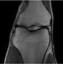
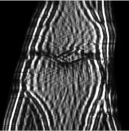
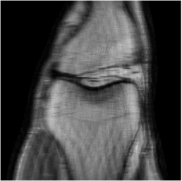
(a)	(b)	(c)	(d)

Figure 1: (a) Reconstructed image from clean measurements. (b) Reconstructed image from measurements with worst-case additive perturbations ($\epsilon=0.004$). (c) Reconstructed image from measurements with 2x undersampling rate during testing (trained with 4x undersampling). (d) Reconstructed image from measurements with a 25% sampling mask shift between training and testing.

3.3 Score-based Diffusion Models

By employing the formulation of the Variance Exploding Stochastic Differential Equation (VE-SDE) [33], we can obtain the stochastic forward and backward processes of score-based DMs as solutions to

$$d\mathbf{z}=\sqrt{\frac{d\sigma^{2}(t)}{dt}}d\mathbf{w}\>,$$ (4)

$$d\mathbf{z}=-\frac{d\sigma^{2}(t)}{dt}\nabla_{\mathbf{z}}\log p_{t}(\mathbf{z})dt+\sqrt{\frac{d\sigma^{2}(t)}{dt}}d\bar{\mathbf{w}}\>,$$ (5)

respectively. In Equations (4) and (5), $t$ spans the interval $[0,1]$ and represents the time index. $d\mathbf{w}$ and $d\bar{\mathbf{w}}$ represent standard Brownian motion evolving forward and backward in time, respectively. The function $\sigma(t)=\sigma_{l}(\sigma_{u}/\sigma_{l})^{t}$ is a monotonically increasing function w.r.t. $t$, where $\sigma_{l}\in(0,1)$ and $\sigma_{u}>1$ are constants. The term $p_{t}(\mathbf{z})$ denotes the distribution of $\mathbf{z}$ at time $t$, while $\nabla_{\mathbf{z}}\log p_{t}(\mathbf{z})$ represents the score function. This score function is replaced by a neural network denoted as $s:\mathbb{C}^{n}\times[0,1]\rightarrow\mathbb{C}^{n}$, parameterized by $\phi$, which is trained using the denoising score matching technique [20] as

$$\underset{\phi}{\min}~{}\mathbb{E}\Bigg{[}\left\|\sigma(t)s_{\phi}(\mathbf{z}(t),t)-\frac{\mathbf{z}(t)-\mathbf{z}}{\sigma(t)}\right\|^{2}\Bigg{]}\>.$$ (6)

The expectation in (6) is taken over $t\sim U[0,1]$, $\mathbf{z}\sim p(\mathbf{z})$, and $\mathbf{z}(t)\sim\mathcal{N}(\mathbf{z},\sigma(t)\mathbf{I})$, where $p(\mathbf{z})=p_{0}(\mathbf{z})$ is the distribution of the training data.

Utilizing a trained DM with $\phi$, the task of sampling $\hat{\mathbf{z}}(0)$ at the time instant $t=0$ is realized through the solution of the reverse process SDE in (5). In this step, the score function is substituted with the learned function $s_{\phi}$. There exist various techniques for sampling from DMs, which involve solving the reverse SDE in (5). In this paper, the Euler method [34] and the Predictor-Corrector (PC) scheme [35] are used. Following the work in [20], a data consistency step is considered to allow sampling from the conditional distribution $p(\mathbf{z}|\mathbf{y})$, which is required when solving inverse imaging problems with DMs. In practice, the continuous time index $t\in[0,1]$ is discretized into $i\in[N_{{r}}]$, where $[N_{{r}}]:=\{1,\dots,N_{r}\}$. The PC sampling technique consists of $N_{r}$ prediction reverse steps. In each prediction iteration, $M_{r}$ correction steps are required [33]. The full procedure is outlined in Algorithm 1.

Algorithm 1 Predictor-Corrector Sampling with DC [20]

Input: Image $\mathbf{z}=\mathbf{A}^{H}\mathbf{y}$, trained DM $s_{\phi}$, discretized time step $N_{r}$, and noise schedule $\epsilon_{i}$.
Function: $\hat{\mathbf{z}}=\operatorname{PCDC}\big{(}s_{\phi}(\mathbf{z}(N_{r}),N_{r}),\mathbf{y},\mathbf{A},N_{r},0\big{)}$.
1: Initialize $\mathbf{z}(N_{r})\sim\mathcal{N}(0,\sigma^{2}(N_{r})\mathbf{I})$.
2: For $i\in\{N_{r}-1,\dots,0\}$ \\Prediction
3:    $\mathbf{z}^{\prime}(i)\leftarrow\mathbf{z}(i+1)+(\sigma^{2}(i+1)-\sigma^{2}(i))s_{\phi}(\mathbf{z}(i+1),i+1)$
4:    $\mathbf{z}(i)\leftarrow\mathbf{z}^{\prime}(i)+\sqrt{\sigma^{2}(i+1)-\sigma^{2}(i)}\eta,~{}\eta\sim\mathcal{N}(0,\mathbf{I})$
5:    $\mathbf{z}(i)\leftarrow\mathbf{z}(i)+\mathbf{A}^{H}(\mathbf{y}-\mathbf{A}\mathbf{z}(i))$ \\Data Consistency
6:    For $M_{r}$ steps do \\  Correction
7:      $\mathbf{z}^{\prime}(i)\leftarrow\mathbf{z}(i)+\epsilon_{i}s_{\phi}(\mathbf{z}(i),i)$
8:      $\mathbf{z}^{\prime}(i)\leftarrow\mathbf{z}^{\prime}(i)+\sqrt{2\epsilon_{i}}~{}\eta,~{}\eta\sim\mathcal{N}(0,\mathbf{I})$
9:      $\mathbf{z}(i)\leftarrow\mathbf{z}^{\prime}(i)+\mathbf{A}^{H}(\mathbf{y}-\mathbf{A}\mathbf{z}(i))$ \\Data Consistency
10: $\hat{\mathbf{z}}=\mathbf{z}(0)$

4 Diffusion Purification for Robust DL-based MRI Reconstruction

In this section, we begin by outlining the key components of the proposed Diffusion Purification (DP) pipeline. Subsequently, we introduce our approach for obtaining the PST step. Following that, we elaborate on our fine-tuning strategy for MoDL, leveraging the purified samples.

4.1 DM-based Purification

Here, we present our DP approach, which consists of the following two stages.

Diffusion Stage: Given measurements $\mathbf{y}$, let $\mathbf{z}_{\textrm{pert}}$ denote the perturbed version of $\mathbf{z}=\mathbf{A}^{H}\mathbf{y}$. As illustrated in the previous section, this perturbed version can be due to various reasons such as random measurement noise, not well-modeled noise and artifacts (e.g., it may make sense to consider worst-case additive noise (from (3))), and different k-space undersampling factors or sampling patterns/masks at testing time. The first stage of the DP approach involves diffusing $\mathbf{z}(0)=\mathbf{z}_{\textrm{pert}}$ from $t=0$ to $t=t^{*}$, where $t^{*}\in(0,1)$ indicates the diffusion time index at which the forward process stops. We term $t^{*}$ as the Process-Switching Time (PST) step. The PST step and $\sigma(\cdot)$ control the amount of noise added to $\mathbf{z}_{\textrm{pert}}$. This stage corresponds to

$$\mathbf{z}_{\textrm{pert}}(t^{*})=\mathbf{z}_{\textrm{pert}}+\sqrt{\sigma^{2}(t^{*})-\sigma^{2}(0)}\eta_{t^{*}}\>,\eta_{t^{*}}\sim\mathcal{N}(0,\mathbf{I})\>.$$ (7)

Purification Stage: After obtaining the diffused perturbed image, denoted as $\mathbf{z}_{\textrm{pert}}(t^{*})$, the objective of the second step is to derive the purified sample, denoted as $\mathbf{z}^{\textrm{pur}}_{\textrm{pert}}$, from $\mathbf{z}_{\textrm{pert}}(t^{*})$. This is achieved by employing the PC reverse process with data consistency (DC). In other words, we use the PC with DC procedure in Algorithm 1 as:

$$\mathbf{z}^{\textrm{pur}}_{\textrm{pert}}(0)=\operatorname{PCDC}\big{(}s_{\phi}(\mathbf{z}_{\textrm{pert}}(t^{*}),t^{*}),\mathbf{y}_{\textrm{pert}},\mathbf{A},t^{*},0\big{)}\>.$$ (8)

In practice, we use $N_{t^{*}}$, which represents the discrete PST step. We remark that $N_{t^{*}}$ is less than the total number of available steps in standard sampling reverse process $N_{r}$. Algorithm 2 illustrates the diffusion purification procedure.

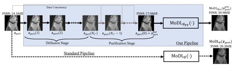
Figure 2: A schematic block diagram illustrating the standard pipeline and our proposed reconstruction pipeline. The functions $\operatorname{MoDL}_{\theta}(\cdot)$ and $\operatorname{MoDL}_{\theta_{\textrm{FT}}}(\cdot)$ represent the application of the standard pre-trained MoDL procedure and our ’pre-trained+fine-tuned’ robust MoDL procedure, respectively.

Intuition: Starting with a perturbed image $\mathbf{z}_{\textrm{pert}}$, which is assumed to be drawn from distribution $q(\mathbf{z})$, our approach initiates with $\mathbf{z}(0)=\mathbf{z}_{\textrm{pert}}$ and gradually introduces noise. If the aliased image $\mathbf{z}$ follows a distribution $p(\mathbf{z})$, then as $t\rightarrow 1$, these two distributions will get closer. This signifies that the perturbations are progressively diminishing due to the incremental noise incorporated during the forward process of (7). To emphasize this point, we present the following theorem where we defer the proof to the Appendix.

Theorem 1. Let $p_{t}(\mathbf{z})$ and $p_{0t}(\mathbf{z}(t)\mid\mathbf{z})$ be the distribution and the conditional distribution of $\mathbf{z}(t)$ given the VE-SDE forward process of (4) starts at the unperturbed image $\mathbf{z}$. Similarly, let $q_{t}(\mathbf{z})$ and $q_{0t}(\mathbf{z}(t)\mid\mathbf{z}_{\textrm{pert}})$ be the distribution and the conditional distribution of $\mathbf{z}(t)$ given the VE-SDE forward process of (4) starts at the perturbed image $\mathbf{A}^{H}\mathbf{y}_{\textrm{pert}}=\mathbf{A}^{H}(\mathbf{y}+\bm{\delta})$. Then, as $t$ moves forward from $t=0$ to $t=1$:

1. The KL divergence between $p_{0t}$ and $q_{0t}$, defined in (9), monotonically decreases.

   $$D_{\textrm{KL}}(p_{0t}\mid\mid q_{0t})=\frac{\|\mathbf{A}^{H}\bm{\delta}\|^{2}}{2(\sigma^{2}(t)-\sigma^{2}(0))}\>,t\in(0,1]\>.$$ (9)

2. The KL divergence between $p_{t}$ and $q_{t}$ monotonically decreases, i.e.,

   $$\frac{dD_{\textrm{KL}}(p_{t}\mid\mid q_{t})}{dt}\leq 0\>.$$ (10)

Algorithm 2 Diffusion Purification

Input: Perturbed measurements $\mathbf{y}_{\textrm{pert}}$, operator $\mathbf{A}$, trained DM $s_{\phi}$, and PST step $N_{t^{*}}$
Function: $\mathbf{z}^{\textrm{pur}}_{\textrm{pert}}=\operatorname{DP}_{\phi}(\mathbf{y}_{\textrm{pert}},\mathbf{A},N_{t^{*}})$.
1: Initialize $\mathbf{z}(0)=\mathbf{z}_{\textrm{pert}}$
2: For $i\in\{1,\dots,N_{t^{*}}\}$ \\Diffusion steps
3:    Obtain $\mathbf{z}(i)\leftarrow\mathbf{z}(i-1)+\sqrt{\sigma^{2}(i)-\sigma^{2}(i-1)}~{}\eta,\eta\sim\mathcal{N}(0,\mathbf{I})$
4: For $i\in\{N_{t^{*}},\dots,1\}$ \\Purification steps
5:    Obtain $\mathbf{z}(i-1)\leftarrow\operatorname{PCDC}(s_{\phi}(\mathbf{z}(i),i),\mathbf{y}_{\textrm{pert}},\mathbf{A},i,i-1)$
6: Obtain $\mathbf{z}^{\textrm{pur}}_{\textrm{pert}}=\mathbf{z}(0)$.

4.2 Selection of the Process-Switching Time Step

In this subsection, we present an approximate method to obtain $t^{*}<1$ (or $N_{t^{*}}<N_{r}$) based on the Maximum Mean Discrepancy (MMD) metric [29].

We utilize the MMD metric to approximately quantify the empirical distribution shift between the original distribution $p(\mathbf{z})$ and the perturbed images’ distribution $q(\mathbf{z})$. During the forward diffusion process, let $Z(i)$ and $Z_{\textrm{p}}(i)$ (with $|Z(i)|=|Z_{\textrm{p}}(i)|$) represent the set of unperturbed and perturbed images, respectively, at discrete time step $i$, where $|\cdot|$ denotes the cardinality of a set. Since we lack access to the exact distributions, we can approximate $\operatorname{MMD}(p_{i},q_{i})$ using empirical distributions as follows:

$$\operatorname{MMD}(p_{i},q_{i})\approx C\Big{(}\sum_{\mathbf{z}(i),\mathbf{z}^{\prime}(i)\in Z(i),\mathbf{z}(i)\neq\mathbf{z}^{\prime}(i)}k(\mathbf{z}(i),\mathbf{z}^{\prime}(i))+\sum_{\mathbf{z}(i),\mathbf{z}^{\prime}(i)\in Z_{\textrm{p}(i)},\mathbf{z}(i)\neq\mathbf{z}^{\prime}(i)}k(\mathbf{z}(i),\mathbf{z}^{\prime}(i))\Big{)}$$ (11)

$$-\frac{2}{|Z(i)|^{2}}\sum_{\mathbf{z}(i)\in Z(i),\mathbf{z}^{\prime}(i)\in Z_{\textrm{p}}(i)}k(\mathbf{z}(i),\mathbf{z}^{\prime}(i))\>,$$

where $C=1/(|Z(i)|(|Z(i)|-1))$ is used for brevity, and $k(\mathbf{z}(i),\mathbf{z}^{\prime}(i))=\exp(-\|\mathbf{z}(i)-\mathbf{z}^{\prime}(i)\|^{2}/2v^{2})$ is the Gaussian kernel parameterized by $v>0$.

Considering the balance between purifying additive perturbations (achieved with a larger $t^{*}$) and preserving global structures (achieved with a smaller $t^{*}$) within perturbed samples, there exists an ideal value of $t^{*}$ that yields a significantly robust reconstruction accuracy. In the case of the worst-case additive perturbations, the changes are usually small and can be rectified with a small $t^{*}$. It was shown in [19] that the most efficient choice of $t^{*}$ related to adversarial robustness tends to be on the smaller side. As such, our objective is to find the minimum value of $i\in[N_{r}]$ for which $\operatorname{MMD}(p_{i},q_{i})\approx 0$. Consequently, we formulate the following optimization problem to determine the near-optimal discrete PST step, $N_{t^{*}}$.

$$N_{t^{*}}:=\big{\{}\underset{i\in[N_{r}]}{\arg\min}~{}i~{}~{}\text{s.t.}~{}~{}\operatorname{MMD}(p_{i},q_{i})=0\big{\}}\>.$$ (12)

In order to obtain the solution of (12), it is required to perform the forward diffusion (steps 2 and 3 in Algorithm 2) on the unperturbed and perturbed samples until the constraint is satisfied.

Since we have knowledge of the source of perturbations that allows us to obtain $Z_{\textrm{p}}$ from $Z$, we remark that the PST step selection method we propose can be applied to any diffusion purification task.

4.3 MoDL Fine-tuning with Purified Perturbed Examples

In this subsection, drawing inspiration from the widely used ‘pre-training + fine-tuning’ approach [36, 18], we propose fine-tuning the parameters of MoDL, which are obtained through the process outlined in Section 3.A, using contaminated purified examples.

We start with pre-trained parameters $\theta$, and utilize noised purified examples for fine-tuning. Let $\theta_{\textrm{FT}}$ represent the fine-tuned parameters specific to MoDL. Initially, we set $\theta_{\textrm{FT}}$ equal to $\theta$. Then, for each measurement $\mathbf{y}$ within dataset $D$, we generate a contaminated variant of the aliased reconstruction, $\mathbf{A}^{H}(\mathbf{y}+\mathbf{v})$, where $\mathbf{v}$ is drawn from a normal distribution $\mathcal{N}(0,\sigma_{\textrm{FT}}\mathbf{I})$. Subsequently, for every $(\mathbf{y},\mathbf{x})$, we follow the procedure outlined in [3], while initializing $\mathbf{x}_{0}$ as

$$\mathbf{x}_{0}=\operatorname{DP}_{\phi}(\mathbf{y}+\mathbf{v},\mathbf{A},N_{t^{*}})\>.$$ (13)

Having trained $\theta_{\textrm{FT}}$ that maps $\mathbf{x}_{0}$ to fully-sampled reconstructions, at the testing phase, the robust MoDL MRI reconstruction using diffusion purification is represented in Algorithm 3. A block diagram of the proposed approach is given in Figure 2.

Algorithm 3 Our Robust MoDL Pipeline

Input: Perturbed measurements $\mathbf{y}_{\textrm{pert}}$, operator $\mathbf{A}$, trained DM $s_{\phi}$, PST step $N_{t^{*}}$, number of unrolling steps $N$, and fine-tuned MoDL parameters $\theta_{\textrm{FT}}$.
Output: Reconstructed image after purification $\mathbf{x}$.
1: Obtain $\mathbf{z}^{\textrm{pur}}_{\textrm{pert}}=\operatorname{DP}_{\phi}(\mathbf{y}_{\textrm{pert}},\mathbf{A},N_{t^{*}})$.
2: Initialize MoDL reconstructed image as $\mathbf{x}_{0}=\mathbf{z}^{\textrm{pur}}_{\textrm{pert}}$
3: For $j\in\{0,\dots,N-1\}$ \\MoDL unrolling steps
4:    Obtain $\mathbf{z}_{j}\leftarrow f_{\theta_{\textrm{FT}}}(\mathbf{x}_{j})$
5:    Obtain $\mathbf{x}_{j+1}\leftarrow(\mathbf{A}^{H}\mathbf{A}+\lambda\mathbf{I})^{-1}(\mathbf{z}^{\textrm{pur}}_{\textrm{pert}}+\lambda\mathbf{z}_{j})$
6: Obtain $\mathbf{x}\leftarrow\mathbf{x}_{N}$

It is worth noting that the fine-tuning approach presented in this paper involves generating noisy samples with additive Gaussian perturbations. This computational process is significantly more efficient than the requirement of fine-tuning with solving Equation (3) used in our recent short study [30].

5 Experimental Results

In this section, we first present our experimental setup and the perturbation sources we consider in this work. Second, we present a study of the selection of the PST step using our MMD-based method. Third, we present our main robustness results, followed by a few ‘not cherry picked’ visualizations of the knee and brain MRI reconstructed images.

5.1 Experimental Setup

In the case of MoDL, we employ a configuration with $N=6$ unrolling steps and a regularization parameter $\lambda=1$. The architecture of $f_{\theta}$ is selected as the Deep Iterative Down-Up Network [37]. Additionally, we set the convergence threshold for the conjugate gradient optimization used in the data consistency step of (2) to $10^{-6}$. In the DM setting, $t\in[0,1]$ is discretized into $500$ steps. We adopt a pre-trained DM model from [20], where $\sigma(i)$ is a geometric series selected as $\sigma(i)=0.01(37800)^{\frac{i}{N_{r}-1}}$. We note that the DM model was trained on the knee training dataset. We conduct our experiments on the fastMRI dataset [38], using 3000 purified images for fine-tuning the pre-trained MoDL network. Additionally, 20 images are reserved for validation, and 64 images are used for testing. Moreover, we use $\sigma_{\textrm{FT}}=0.01$. The multi-coil image data is acquired using $15$ coils and is cropped to a resolution of $320\times 320$ pixels for MRI reconstruction. To simulate undersampling of the MRI k-space, we adopt a Cartesian mask with 4x acceleration (equivalent to a 25% sampling rate). Sensitivity maps for the coils, which are incorporated into the operator $\mathbf{A}$ for all scenarios, are obtained using the BART toolbox [39]. Rather than employing the root-sum-of-squares reconstruction method, we apply sensitivity map-based reconstruction. The quality of the reconstructed images is evaluated using the Peak Signal-to-Noise Ratio (PSNR) in dB, and the Structural Similarity Index Measure (SSIM), which returns values in $[0,1]$ with $1$ indicating identical images. Our code is made available online.

For the purpose of baseline comparison, we utilize AT and RS. In AT, we implemented a 30-step PGD procedure within its minimax formulation. In the case of end-to-end (E2E) RS, we introduced Gaussian noise with a standard deviation of $0.01$, and to perform the smoothing operation, we employed 10 Monte Carlo samplings.

Figure 3: Selection of the PST step. Estimated MMD (using (11)) w.r.t. the discrete steps $i\in[N_{r}]$ (top). Ablation study by comparing with the ground truth (bottom).

Sources of Instabilities: In this paper, we assess the robustness of our proposed pipeline by examining two main categories of perturbations. The first category involves additive perturbations applied to $\mathbf{y}$. Recall that this is both an input to the unrolled MoDL and is used in the conjugate gradients (CG) scheme in the data consistency step. Within the additive perturbations category, we introduce two types of additive noise: a zero-mean Gaussian random vector with a variance of $0.01$ and worst-case additive perturbations. For the latter, we employed two gradient-based attack techniques. The first method is the conventional $\ell_{\infty}$-norm PGD [15] with 30 iterations and a perturbation budget of $\epsilon=0.004$. The second approach utilizes the advanced momentum-based AUTO attack [40], configured similarly to PGD. To generate perturbations using PGD or AUTO, it is necessary to calculate the gradients w.r.t. the input of our model. In our recent work [30], we computed the gradients with only propagating through MoDL. In this paper, we consider an additional case where we apply the method from [19] and calculate the gradients to propagate through both MoDL and the SDE of the DP. This represents the worst-case additive perturbations w.r.t. the DP and MoDL. In this case, the perturbations are generated as:

$$\underset{\|\bm{\delta}\|_{\infty}\leq\epsilon}{\max}~{}\mathcal{L}\Big{(}\operatorname{MoDL}_{\theta_{\textrm{FT}}}(\mathbf{A}^{H}\mathbf{y}),\operatorname{MoDL}_{\theta_{\textrm{FT}}}(\operatorname{DP}_{\phi}(\mathbf{A}^{H}(\mathbf{y}+\bm{\delta}),N_{t^{*}}))\Big{)}\>.$$ (14)

Table 1: Knee dataset Reconstruction accuracy. The symbol $\uparrow$ indicates that a higher value corresponds to an improved reconstruction accuracy. The result $a$$\pm b$ represents the mean ($a$) and standard deviation ($b$).

Models	Clean Accuracy		Robust Accuracy (Evaluated by random noise)		Robust Accuracy (Evaluated by PGD)		Robust Accuracy (Evaluated by AUTO)
Metrics	PSNR $\uparrow$	SSIM $\uparrow$	PSNR $\uparrow$	SSIM $\uparrow$	PSNR $\uparrow$	SSIM $\uparrow$	PSNR $\uparrow$	SSIM $\uparrow$
Vanilla MoDL	32.74$\pm$1.57	0.921$\pm$0.08	31.67$\pm$1.32	0.915$\pm$0.08	24.78$\pm$1.42	0.769$\pm$0.08	24.28$\pm$1.28	0.761$\pm$0.07
E2E-RS	-0.12$\pm$1.24	-0.006$\pm$0.08	+0.23$\pm$1.24	+0.01$\pm$0.08	1.62$\pm$1.70	+0.034$\pm$0.09	1.51$\pm$1.70	+0.031$\pm$0.09
AT	-0.52$\pm$2.07	-0.008$\pm$0.09	+0.1$\pm$1.24	+0.004$\pm$0.08	+5.62$\pm$1.24	+0.093$\pm$0.10	+5.44$\pm$1.22	+0.091$\pm$0.11
DP+MoDL	+0.81$\pm$2.06	+0.011$\pm$0.09	+1.66$\pm$2.06	+0.021$\pm$0.09	+8.47$\pm$0.95	+0.148$\pm$0.1	+8.92$\pm$0.96	+0.152$\pm$0.1

Table 2: Brain dataset Reconstruction accuracy. The symbol $\uparrow$ indicates that a higher value corresponds to an improved reconstruction accuracy. The result $a$$\pm b$ represents the mean ($a$) and standard deviation ($b$)..

Models	Clean Accuracy		Robust Accuracy (Evaluated by random noise)		Robust Accuracy (Evaluated by PGD)		Robust Accuracy (Evaluated by AUTO)
Metrics	PSNR $\uparrow$	SSIM $\uparrow$	PSNR $\uparrow$	SSIM $\uparrow$	PSNR $\uparrow$	SSIM $\uparrow$	PSNR $\uparrow$	SSIM $\uparrow$
Vanilla MoDL	33.11$\pm$3.27	0.918$\pm$0.07	31.89$\pm$2.47	0.899$\pm$0.07	25.18$\pm$2.42	0.774$\pm$0.07	24.67$\pm$1.98	0.77$\pm$0.08
RS-E2E	-0.24$\pm$3.24	-0.002$\pm$0.07	+0.51$\pm$3.24	+0.014$\pm$0.07	+0.77$\pm$2.70	+0.028$\pm$0.08	+1.08$\pm$2.70	+0.033$\pm$0.09
AT	-1.44$\pm$3.01	-0.001$\pm$0.08	+0.23$\pm$3.22	+0.002$\pm$0.07	+4.56$\pm$1.22	+0.088$\pm$0.11	+4.45$\pm$1.22	+0.091$\pm$0.10
DP+MoDL	+0.77$\pm$2.88	+0.02$\pm$0.08	+1.46$\pm$2.56	+0.023$\pm$1.08	+7.56$\pm$0.25	+0.131$\pm$0.12	+8.67$\pm$1.28	+0.14$\pm$0.12

In the second category, we evaluate the robustness of our approach by considering two variations in the construction of the forward operator $\mathbf{A}$ between the training and testing phases. The first variation involves using a different acceleration factor (sampling rate), while the second involves shifts in the locations of the k-space sampling. Phrased differently, we train MoDL with $\mathbf{A}$ and evaluate it with different $\mathbf{A}_{\textrm{test}}$. Robustness to such instabilities would be very useful for deployed deep MRI reconstruction methods.

5.2 Selection of the PST Step

In this section, we conduct an experiment to demonstrate the effectiveness of our MMD-based method in determining the near-optimal PST step, denoted as $N_{t^{*}}$. The experiment is depicted in Figure 3 (top), where we present the MMD values computed using (11). Additionally, Figure 3 (bottom) displays the results obtained when applying various values of $N_{t^{*}}$ within our pipeline, with corresponding PSNR values compared to ground truth images. In this experiment, we calculate the MMD values by setting the Gaussian kernel $v$ as the mean of the magnitude of the images in set $Z$, which comprises images $\mathbf{A}^{H}\mathbf{y}$ for 20 scans $\mathbf{y}\in D$. For the perturbed images, we utilize the worst-case additive perturbations, denoted as $\bm{\delta}$, calculated from (3). Consequently, the set $Z_{\textrm{p}}$ encompasses $\mathbf{A}^{H}(\mathbf{y}+\bm{\delta})$ for the same measurements used in $Z$.

Analysis of Figure 3 (bottom) reveals that, in comparison to the ground truth, the optimal PSNR result is achieved at $N_{t^{*}}=150$, consistent with the observed approximate MMD value in Figure 3 (top). Furthermore, it is evident that although the MMD values for $N_{t^{*}}$ in the range $(150,500]$ are also close to zero, PSNR values begin to deteriorate. This observation aligns with the intuition that increasing the value of $N_{t^{*}}$ effectively removes perturbations but runs the risk of losing image structure. Consequently, for the remainder of this paper, we adopt $N_{t^{*}}=150$ as our chosen setting.

Furthermore, we remark that the number of reverse (purification) process steps chosen for our robustification task, which is 150, is notably lower than the requirement in the diffusion-based image reconstruction task presented in [20], where 500 steps were used.

5.3 Robustness Results

Figure 4: Robustness evaluation against variations in: (a) acceleration factors, (b) locations of k-space sampling, (c) variance level of the Gaussian random additive noise, and (d) perturbation budget of the worst-case additive disturbances generated by PGD and AUTO methods. The ‘PGD E2E’ and ‘AUTO E2E’ in (d) correspond to the cases of generating end-to-end perturbations while calculating gradients through propagating the DP and MoDL. Furthermore, ‘Ours PGD w/out FT’ corresponds to the case where no MoDL fine-tuning is applied. This figure is best viewed in color.

Ground Truth	MoDL	RS-E2E	AT	Ours
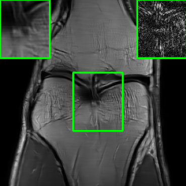
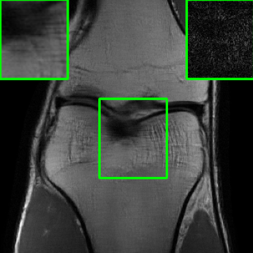
PSNR = $\infty$ dB	PSNR = 22.28 dB	PSNR = 25.34 dB	PSNR = 29.47 dB	PSNR = 32.88 dB
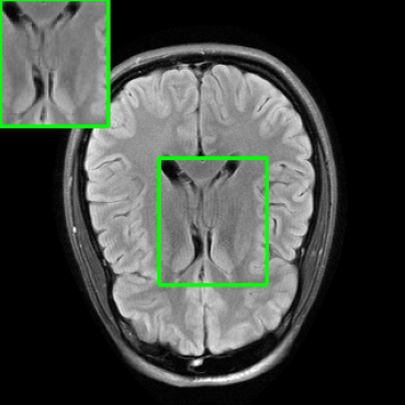
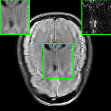
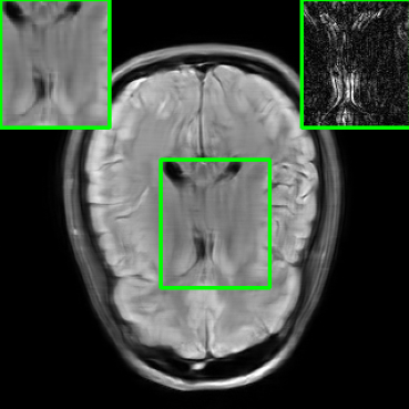
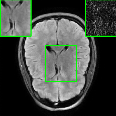
PSNR = $\infty$ dB	PSNR = 22.23 dB	PSNR = 24.56 dB	PSNR = 29.25 dB	PSNR = 33.18 dB

Figure 5: Visualization of ground-truth and reconstructed images using different methods, evaluated by PGD-based worst-case additive perturbations with $\epsilon=0.004$.

Table 1 provides a comprehensive view of the relative performance of our robustification method, as well as AT and E2E-RS, assessed through PSNR and SSIM metrics using the knee dataset. We evaluate these methods across multiple scenarios, including benign aliased images (columns 2 and 3), images subjected to additive random Gaussian noise with variance of $0.01$ (columns 4 and 5), and images with additive worst-case perturbations generated using PGD and AUTO methods with $\epsilon=0.002$ (columns 6 to 9).

While both AT and RS show improvements when compared to vanilla MoDL, we observe that our robustification approach excels in achieving the highest level of robust accuracy. Additionally, the results in the second and third columns highlight the effectiveness of our approach in enhancing MoDL reconstruction performance, even in the absence of any perturbations.

In Table 2, we replicate the experiment conducted in Table 1, this time utilizing the brain dataset. Notably, MoDL underwent fine-tuning using perturbed purified examples sourced from the training set of the brain data.

When comparing the results of our proposed method with other robustification approaches, we find that similar observations remain consistent. An important point to highlight is that the pre-trained DM employed in our purification stage for this experiment was originally trained exclusively on knee data, without any exposure to brain data. This underscores the robust generalization capabilities of the diffusion purification process within our approach, extending its effectiveness to previously unseen MRI datasets.

It’s worth mentioning that similar diffusion model generalization capabilities were also observed in the study conducted by Chung et al. [20]. However, further thorough investigation is required to precisely determine the limitations of these generalization capabilities, and this remains a promising direction for future research.

In Figure 4, we present the PSNR performance of AT, E2E-RS, and our method, evaluated using the noise sources outlined in Section V.B. In Figure 4(a), we illustrate performance across different acceleration factors. During training, a k-space undersampling or acceleration factor of 4x was employed. However, during testing, we assess performance with various acceleration factors ranging from 2x to 8x. It is evident that when the acceleration factor matches the training phase (4x), all methods exhibit their highest PSNR results compared to when different acceleration factors are used. Nevertheless, when compared to the other methods, our approach consistently achieves the highest PSNR values when tested with acceleration factors other than 4x. For instance, at 2x acceleration, all methods report PSNR values of 21 dB or lower, while our approach achieves nearly 30 dB, highlighting its superior performance in such scenarios.

Figure 4(b) shows the PSNR values of AT, E2E-RS, and our approach, assessed under varying percentages of shifts in the location of the k-space sampling during testing. The shifts were applied to high-frequency phase encode locations in the original sampling pattern or mask. This is to help understand reconstruction robustness when the sampling masks change a lot at a fixed k-space undersampling factor. We observe that as the percentage of shifts increases, the reported PSNR values decrease across all methods. Remarkably, our method consistently outperforms the others across all tested percentages, exhibiting the highest PSNR values. This superior performance underscores the improved robustness of our approach in the face of very different sampled lines at a given sampling budget.

In Figure 4(c), we present the PSNR values of AT, E2E-RS, and our approach, evaluated under different levels of added Gaussian noise during testing. Notably, as the noise level (indicated by the variance) increases, the reported PSNR values decrease for all methods. However, our approach outperforms the others across all tested noise levels, consistently exhibiting the highest PSNR values. This remarkable performance highlights the robustness of our approach in dealing with additive noise.

In Figure 4(d), we present the PSNR performance of AT, E2E-RS, and our approach, evaluated under varying perturbation budgets given by the values of $\epsilon$. The evaluation encompasses both PGD and AUTO methods. Additionally, we explore the PGD E2E and AUTO E2E scenarios, which involve generating end-to-end perturbations using (14) . As the perturbation budget increases, all methods experience a decline in their PSNR values, which is expected. However, it’s noteworthy that our approach consistently exhibits the best performance across the entire range of perturbation budgets. We also observe that employing the E2E attack results in slightly lower PSNR values compared to the case of generating perturbations solely w.r.t. MoDL. Finally, we observe that the AUTO results are marginally lower than those of PGD, which aligns with expectations since AUTO represents a more advanced adversary finding approach.

Moreover, in Figure 4(d), we illustrate the effect of fine-tuning on the robustness of our method. Specifically, we compare PSNR values for our DP approach when exposed to PGD-based worst-case additive perturbations under two scenarios: with fine-tuning MoDL using perturbed purified training samples (i.e., $f_{\theta_{\textrm{FT}}}$) and without fine-tuning, relying solely on the pre-trained MoDL (i.e., $f_{\theta}$). These two cases are represented by the solid blue and black plots in Figure 4(d). The results clearly highlight that the pre-trained+fine-tuned MoDL enhances robustness, as evidenced by the higher PSNR values compared to pre-trained MoDL. We also note that the results obtained without fine-tuning are slightly higher than those achieved using AT (see the solid green plot in Figure 4(d)). This indicates that MoDL+DP without fine-tuning still exhibits improvements when compared to AT, vanilla MoDL, and RS-E2E.

5.4 Visualizations

We now present visual samples from both the knee and brain datasets. Specifically, Figure 5 presents visual comparison of image reconstructions and their associated reconstruction errors within a closely examined region. Each image in the figure includes two inset panels in the top-left and top-right corners. The top-left inset panel, enclosed within a green bounding box, serves as a reference for the region of interest in the image. In contrast, the top-right inset panel depicts an error map in relation to the ground truth. Notably, our method stands out in its ability to capture the original image’s features, surpassing the performance of alternative methods (as also evident from the reported PSNR values). This visual comparison underscores the superior quality and accuracy of our approach in the robustification of the MRI image reconstruction task.

6 Conclusion & Future work

Recent studies have unmasked vulnerabilities in DL-based MRI reconstruction methods—namely, susceptibility to additive perturbations and variations in training/testing settings, such as acceleration factors and k-space sampling patterns. This paper has addressed these challenges by harnessing the power of diffusion models. Our innovative robustification strategy significantly enhanced the resilience of DL-based MRI reconstruction models by integrating pre-trained diffusion models as noise purifiers. Unlike conventional robustification techniques like adversarial training (AT), our method eliminated the need for complex minimax optimization problems. Instead, it simply requires fine-tuning on perturbed purified examples. Our extensive experiments have illustrated the remarkable efficacy of our approach in mitigating different instabilities when compared to leading robustification methods, including AT and randomized smoothing. These findings underscore the promise of leveraging diffusion models to enhance the robustness and reliability of DL-based MRI reconstruction, paving the way for more dependable and accurate medical imaging technologies in the future.

For future research directions, we intend to thoroughly explore the various noise sources and models that diffusion-based purification methods can effectively manage within the realm of MR imaging and other modalities. Additionally, we are eager to investigate the boundaries and potentials of the generalization capabilities inherent to diffusion-based noise purifiers. These inquiries will offer valuable insights into the adaptability and promise of this approach in advancing computational imaging techniques. Furthermore, we intend to investigate the stability of the reverse SDE in the proposed purification procedure starting from the perturbed noisy images’ distribution at the process switching time step.

Appendix A Proof of Theorem 1

For the first part, we begin by establishing the results in (9). Utilizing the VE-SDE formulation of DMs, the conditional distributions $p_{0t}$ and $q_{0t}$ are expressed as per the following equations [33].

$$p_{0t}(\mathbf{z}(t)\mid\mathbf{z})=\mathcal{N}(\mathbf{z}(t);\mathbf{z},(\sigma^{2}(t)-\sigma^{2}(0))\mathbf{I})\>,$$ (15a)

$$q_{0t}(\mathbf{z}(t)\mid\mathbf{z}_{\textrm{pert}})=\mathcal{N}(\mathbf{z}(t);\mathbf{z}_{\textrm{pert}},(\sigma^{2}(t)-\sigma^{2}(0))\mathbf{I})\>.$$ (15b)

Notably, these two distributions have different means, but share the same covariance. Consequently, the $D_{\textrm{KL}}$ can be obtained as

$$D_{\textrm{KL}}(p_{0t}\mid\mid q_{0t})=\frac{1}{2}\bigg{(}\log\Big{(}\frac{\det(\sigma^{2}\mathbf{I})}{\det(\sigma^{2}\mathbf{I})}\Big{)}+\textrm{Tr}\Big{(}(\sigma^{2}\mathbf{I})^{-1}(\sigma^{2}\mathbf{I})\Big{)}$$ (16)

$$+(\mathbf{z}_{\textrm{pert}}-\mathbf{z})^{T}(\sigma^{2}\mathbf{I})^{-1}(\mathbf{z}_{\textrm{pert}}-\mathbf{z})-n\bigg{)}\>,$$

where $\det(\cdot)$ (resp. $\textrm{Tr}(\cdot)$) denotes the determinant (resp. trace) of a matrix, and $\sigma^{2}=\sigma^{2}(t)-\sigma^{2}(0)$ is used for brevity. Since $\log(1)=0$, the first term is zero. Given the definition of the trace and the identity matrix properties, the second term reduces to $n$ and cancels the last term. Since $\mathbf{A}^{H}\bm{\delta}=\mathbf{z}_{\textrm{pert}}-\mathbf{z}$, and $(\mathbf{A}^{H}\bm{\delta})^{T}\mathbf{A}^{H}\bm{\delta}\geq 0$, then Equation (9) holds.

Subsequently, the numerator in (9) is more than or equal to $0$ (can only be zero if $\bm{\delta}=0$), and is not a function of $t$. Moreover, since $\sigma(t)=\sigma_{l}(\sigma_{u}/\sigma_{l})^{t}$, where $\sigma_{l}\in(0,1)$ and $\sigma_{u}>1$ are constants, it is evident that the denominator monotonically increases as $t$ increases.

In conclusion, the rate of change of $D_{\textrm{KL}}(p_{0t}\mid\mid q_{0t})$ w.r.t. $t$ (as long as $\bm{\delta}\neq 0$) is less than $0$. Given the derivative of $\sigma(t)$ w.r.t. $t$ is $\frac{d\sigma(t)}{dt}=\sigma_{l}\log(\sigma_{u}/\sigma_{l})(\sigma_{u}/\sigma_{l})^{t}$, this is supported by

$$\frac{dD_{\textrm{KL}}(p_{0t}\mid\mid q_{0t})}{dt}=\frac{-\|\mathbf{A}^{H}\bm{\delta}\|^{2}\sigma_{l}\log(\sigma_{u}/\sigma_{l})(\sigma_{u}/\sigma_{l})^{2t}}{\big{(}\sigma^{2}(t)-\sigma^{2}_{l}\big{)}^{2}}<0\>.$$ (17)

This inequality establishes that $D_{\textrm{KL}}(p_{0t}\mid\mid q_{0t})$ monotonically decreases as time travels from $t=0$ to $t=1$ while employing the forward process defined in (4). Consequently, the proof of the first part is complete.

The proof of the second part follows from [33] and [19]. Using the Fokker-Planck-Kolmogorov representation [41] for the forward process in (4), we write

$$\frac{dp_{t}(\mathbf{z})}{dt}=\frac{1}{2}\nabla_{\mathbf{z}}\cdot\big{(}p_{t}(\mathbf{z})\frac{d\sigma^{2}(t)}{dt}\nabla_{\mathbf{z}}\log p_{t}(\mathbf{z})\big{)}\>,$$ (18a)

$$\frac{dq_{t}(\mathbf{z})}{dt}=\frac{1}{2}\nabla_{\mathbf{z}}\cdot\big{(}q_{t}(\mathbf{z})\frac{d\sigma^{2}(t)}{dt}\nabla_{\mathbf{z}}\log q_{t}(\mathbf{z})\big{)}\>.$$ (18b)

Employing the definition of the KL divergence, Equation (18), integration by parts, and assuming the smoothness and fast decay of $p_{t}(\mathbf{z})$ and $q_{t}(\mathbf{z})$, we can derive the derivative of the KL divergence w.r.t. $t$:

$$\frac{dD_{\textrm{KL}}(p_{t}\mid\mid q_{t})}{dt}=-\frac{1}{2}\frac{d\sigma^{2}(t)}{dt}D_{\textrm{F}}(p_{t}\mid\mid q_{t})\leq 0\>,$$ (19)

where

$$D_{\textrm{F}}(p_{t}\mid\mid q_{t})=\int p_{t}(\mathbf{z})\|\nabla_{\mathbf{z}}\log p_{t}(\mathbf{z})-\nabla_{\mathbf{z}}\log q_{t}(\mathbf{z})\|^{2}d\mathbf{z}\geq 0\>,$$ (20)

denotes the Fisher divergence. Given that $\frac{d\sigma^{2}(t)}{dt}>0$, the proof of the second part is thereby established.

References

- Lustig et al. [2008] M. Lustig, D. L. Donoho, J. M. Santos, and J. M. Pauly. Compressed sensing mri. IEEE Signal Processing Magazine, 25(2):72–82, 2008. doi: 10.1109/MSP.2007.914728.
- Yang et al. [2010] J. Yang, Y. Zhang, and W. Yin. A Fast Alternating Direction Method for TVL1-L2 Signal Reconstruction From Partial Fourier Data. IEEE Journal of Selected Topics in Signal Processing, 4(2):288–297, 2010. doi: 10.1109/JSTSP.2010.2042333.
- Aggarwal et al. [2018] H. K. Aggarwal, M. P. Mani, and M. Jacob. Modl: Model-based deep learning architecture for inverse problems. IEEE transactions on medical imaging, 38(2):394–405, 2018.
- Schlemper et al. [2019] J. Schlemper, C. Qin, J. Duan, R. M. Summers, and K. Hammernik. Sigma-net: Ensembled iterative deep neural networks for accelerated parallel MR image reconstruction. arXiv preprint arXiv:1912.05480, 2019.
- Ravishankar et al. [2018] S. Ravishankar, A. Lahiri, C. Blocker, and J. A. Fessler. Deep dictionary-transform learning for image reconstruction. In 2018 IEEE 15th International Symposium on Biomedical Imaging (ISBI 2018), pages 1208–1212. IEEE, 2018.
- Schlemper et al. [2018] J. Schlemper, J. Caballero, J. V. Hajnal, A. N. Price, and D. Rueckert. A deep cascade of convolutional neural networks for dynamic MR image reconstruction. IEEE Transaction on Medical Imaging, 37(2):491–503, Feb. 2018. ISSN 1558254X. doi: 10.1109/TMI.2017.2760978.
- Ronneberger et al. [2015] O. Ronneberger, P. Fischer, and T. Brox. U-net: Convolutional networks for biomedical image segmentation. In Medical Image Computing and Computer-Assisted Intervention – MICCAI 2015, pages 234–241, 2015.
- Han and Ye [2018] Y. Han and J. C. Ye. Framing u-net via deep convolutional framelets: Application to sparse-view ct. IEEE Transactions on Medical Imaging, 37(6):1418–1429, 2018. doi: 10.1109/TMI.2018.2823768.
- Lee et al. [2018] D. Lee, J. Yoo, S. Tak, and J. C. Ye. Deep residual learning for accelerated mri using magnitude and phase networks. IEEE Transactions on Biomedical Engineering, 65(9):1985–1995, 2018. doi: 10.1109/TBME.2018.2821699.
- Antun et al. [2020] V. Antun, F. Renna, C. Poon, B. Adcock, and A.C. Hansen. On instabilities of deep learning in image reconstruction and the potential costs of AI. Proceedings of the National Academy of Sciences, 117(48):30088–30095, 2020.
- Zhang et al. [2021] C. Zhang, J. Jia, et al. On instabilities of conventional multi-coil mri reconstruction to small adverserial perturbations. arXiv preprint arXiv:2102.13066, 2021.
- Gilton et al. [2021] D. Gilton, G. Ongie, and R. Willett. Deep equilibrium architectures for inverse problems in imaging. IEEE Transactions on Computational Imaging, 7:1123–1133, 2021.
- Jia et al. [2022] J. Jia, M. Hong, Y. Zhang, M. Akcakaya, and S. Liu. On the robustness of deep learning-based mri reconstruction to image transformations. In Workshop on Trustworthy and Socially Responsible Machine Learning, NeurIPS 2022, 2022.
- Wolf [2019] A. Wolf. Making medical image reconstruction adversarially robust. 2019.
- Madry et al. [2017] A. Madry, A. Makelov, L. Schmidt, D. Tsipras, and A. Vladu. Towards deep learning models resistant to adversarial attacks. arXiv preprint arXiv:1706.06083, 2017.
- Zhang et al. [2019] H. Zhang, Y. Yu, J. Jiao, E. P . Xing, L. E. Ghaoui, and M. I. Jordan. Theoretically principled trade-off between robustness and accuracy. International Conference on Machine Learning, 2019.
- J. Cohenand and Kolter [2019] E. Rosenfeld J. Cohenand and Z. Kolter. Certified adversarial robustness via randomized smoothing. In International Conference on Machine Learning, pages 1310–1320. PMLR, 2019.
- Salman et al. [2020] H. Salman, M. Sun, G. Yang, A. Kapoor, and J. Z. Kolter. Denoised smoothing: A provable defense for pretrained classifiers. Advances in Neural Information Processing Systems, 33, 2020.
- Nie et al. [2022] W. Nie, B. Guo, Y. Huang, C. Xiao, A. Vahdat, and A. Anandkumar. Diffusion models for adversarial purification. In Proceedings of the 39th International Conference on Machine Learning, volume 162 of Proceedings of Machine Learning Research, pages 16805–16827. PMLR, 2022. URL https://proceedings.mlr.press/v162/nie22a.html.
- Chung and Ye [2022] H. Chung and J. C. Ye. Score-based diffusion models for accelerated MRI. Medical image analysis, 80:102479, 2022.
- Chung et al. [2022] H. Chung, J. Kim, M. T.Mccann, M.L . Klasky, and J. C. Ye. Diffusion posterior sampling for general noisy inverse problems. arXiv preprint arXiv:2209.14687, 2022.
- Karras et al. [2022] T. Karras, M. Aittala, T. Aila, and S. Laine. Elucidating the design space of diffusion-based generative models. Advances in Neural Information Processing Systems, 35:26565–26577, 2022.
- Yang et al. [2017] Y. Yang, J. Sun, H. Li, and Z. Xu. ADMM-Net: A Deep Learning Approach for Compressive Sensing MRI. arXiv preprint arXiv:1705.06869, 2017.
- Zhang and Ghanem [2018] J. Zhang and B. Ghanem. ISTA-Net: Interpretable Optimization-Inspired Deep Network for Image Compressive Sensing. arXiv preprint arXiv:1706.07929, 2018.
- Ravishankar et al. [2020] S. Ravishankar, J. C. Ye, and J.A. Fessler. Image reconstruction: From sparsity to data-adaptive methods and machine learning. Proceedings of the IEEE, 108(1):86–109, 2020. doi: 10.1109/JPROC.2019.2936204.
- Hammernik et al. [2023] K. Hammernik, T. Küstner, B. Yaman, Z. Huang, D. Rueckert, F. Knoll, and M. Akçakaya. Physics-driven deep learning for computational magnetic resonance imaging: Combining physics and machine learning for improved medical imaging. IEEE Signal Processing Magazine, 40(1):98–114, 2023. doi: 10.1109/MSP.2022.3215288.
- Ongie et al. [2020] G. Ongie, A. Jalal, C.A. Metzlerand, R.G. Baraniuk, A. G. Dimakis, and R. Willett. Deep learning techniques for inverse problems in imaging. IEEE Journal on Selected Areas in Information Theory, 1(1):39–56, 2020.
- Wong et al. [2020] E Wong, L. Rice, and J. Z. Kolter. Fast is better than free: Revisiting adversarial training. In International Conference on Learning Representations, 2020. URL https://openreview.net/forum?id=BJx040EFvH.
- Gretton et al. [2006] A. Gretton, K. Borgwardt, M. Raschand, B. Schölkopf, and A. Smola. A kernel method for the two-sample-problem. Advances in neural information processing systems, 19, 2006.
- Alkhouri et al. [2023] I. Alkhouri, S. Liang, R. Wang, Q. Qu, and S. Ravishankar. Diffusion-based adversarial purification for robust deep mri reconstruction. arXiv preprint arXiv:2309.05794, 2023.
- Donoho [2006] D.L. Donoho. Compressed sensing. IEEE Transactions on Information Theory, 52(4):1289–1306, 2006. doi: 10.1109/TIT.2006.871582.
- Li et al. [2023] H. Li, J. Jia, S. Liang, Y. Yao, S. Ravishankar, and S. Liu. Smug: Towards robust mri reconstruction by smoothed unrolling. In ICASSP 2023-2023 IEEE International Conference on Acoustics, Speech and Signal Processing (ICASSP), pages 1–5. IEEE, 2023.
- Song et al. [2020] Y. Song, J. Sohl-Dickstein, D.P. Kingma, A. Kumar, S. Ermon, and B. Poole. Score-based generative modeling through stochastic differential equations. arXiv preprint arXiv:2011.13456, 2020.
- Platen and Bruti-Liberati [2010] E. Platen and N. Bruti-Liberati. Numerical solution of stochastic differential equations with jumps in finance, volume 64. Springer Science & Business Media, 2010.
- Allgower and Georg [2012] E. L. Allgower and K. Georg. Numerical continuation methods: an introduction, volume 13. Springer Science & Business Media, 2012.
- Zoph et al. [2020] B. Zoph, G.Ghiasi, T. Lin, Y. Cui, H. Liu, E . D. Cubuk, and Q. Le. Rethinking pre-training and self-training. Advances in Neural Information Processing Systems, 33, 2020.
- Yu et al. [2019] S. Yu, B. Park, and J. Jeong. Deep iterative down-up CNN for image denoising. In Proceedings of the IEEE/CVF Conference on Computer Vision and Pattern Recognition Workshops, pages 0–0, 2019.
- Zbontar et al. [2018] J. Zbontar, F. Knoll, A. Sriram, T. Murrell, Z. Huang, M. J. Muckley, A. Defazio, R. Stern, P. Johnson, M. Bruno, et al. fastMRI: An open dataset and benchmarks for accelerated MRI. arXiv preprint arXiv:1811.08839, 2018.
- Tamir et al. [2016] J. I. Tamir, F. Ong, J. Y. Cheng, M. Uecker, and M. Lustig. Generalized magnetic resonance image reconstruction using the berkeley advanced reconstruction toolbox. In ISMRM Workshop on Data Sampling & Image Reconstruction, Sedona, AZ, 2016.
- Croce and Hein [2020] F. Croce and M. Hein. Reliable evaluation of adversarial robustness with an ensemble of diverse parameter-free attacks, 2020.
- Särkkä and Solin [2019] S. Särkkä and A. Solin. Applied stochastic differential equations, volume 10. Cambridge University Press, 2019.