Entropy current and entropy production in relativistic spin hydrodynamics

Abstract

We use a first-principle quantum-statistical method to derive the expression of the entropy production rate in relativistic spin hydrodynamics. We show that the entropy current is not uniquely defined and can be changed by means of entropy-gauge transformations, much the same way as the stress-energy tensor and the spin tensor can be changed with pseudo-gauge transformations. We show that the local thermodynamic relations, which are admittedly educated guesses in relativistic spin hydrodynamics inspired by those at global thermodynamic equilibrium, do not hold in general and they are also non-invariant under entropy-gauge transformations. Notwithstanding, we show that the entropy production rate is independent of those transformations and we provide a universally applicable expression, extending that known in literature, from which one can infer the dissipative parts of the energy momentum and spin tensors.

I Introduction

Motivated by the evidence of spin polarization of particles produced in relativistic heavy ion collisions [1, 2], there is a growing interest in the so-called relativistic spin hydrodynamics [3, 4, 5, 6, 7, 8, 9, 10, 11, 12, 13, 14, 15, 16, 17, 18, 19]. Relativistic spin hydrodynamics stipulates that the description of a relativistic fluid requires the addition of a spin tensor, that is the mean value of a rank 3 tensor operator ${\widehat{\cal S}}^{\lambda\mu\nu}$ (the last two indices anti-symmetric) contributing to the overall angular momentum current:

$$\widehat{\cal J}^{\lambda\mu\nu}=x^{\mu}{\widehat{T}}^{\lambda\nu}-x^{\nu}{\widehat{T}}^{\lambda\mu}+{\widehat{\cal S}}^{\lambda\mu\nu}\,,$$

where ${\widehat{T}}^{\mu\nu}$ is the stress-energy tensor operator. This current is conserved, which implies that the spin tensor fulfills the continuity equation:

$$\partial_{\lambda}{\widehat{\cal S}}^{\lambda\mu\nu}={\widehat{T}}^{\nu\mu}-{\widehat{T}}^{\mu\nu}\,.$$ (1)

It is important to point out that the spin tensor - and the stress-energy tensor as well - are not uniquely defined. Indeed, they can be changed with a so-called pseudo-gauge transformation [20, 21] to a new couple of tensors fulfilling the same dynamical equations and providing the same integrated conserved charges. Since the spin tensor can be made vanishing with a suitable pseudo-gauge transformation, its dynamical meaning has been questioned, yet it was observed in ref. [22] that for a fluid not in global thermodynamic equilibrium (such as the QGP throughout its lifetime) the quantum state of the system (i.e. the density operator describing initial local equilibrium) is not invariant under pseudo-gauge transformations. Thus, in principle, the physical measurements depend on the pseudo-gauge if the initial quantum state is not invariant, and particularly on the intensive quantity which is thermodynamically conjugated to the spin tensor, the spin potential. For instance, if the spin tensor does not vanish, the spin polarization of final particles depends on the difference between spin potential and thermal vorticity [23]. The microscopic conditions underpinning spin hydrodynamics have been studied and elucidated in ref. [11], where it was made clear that spin hydrodynamics regime occurs under a specific hierarchy of the interaction time scales in the system.

A key problem in the relativistic hydrodynamics with spin is the derivation of the constitutive equations of the spin tensor as well as of the anti-symmetric part of the stress-energy tensor. This problem has drawn significant attention over the past few years, with several derivations of constitutive equations  [7, 8, 9, 10, 11, 12, 13] based on the requirement of the positivity of local entropy production rate. However, like in the traditional approach to relativistic hydrodynamics, the entropy current is not really derived, but it is obtained from an educated guess of a thermodynamic relations between the proper densities of entropy, energy, charge and “spin density” $S^{\mu\nu}\equiv u_{\lambda}{\cal S}^{\lambda,\mu\nu}$ as follows:

$$\begin{split}&Ts+\mu n=\rho+p-\frac{1}{2}\omega_{\mu\nu}S^{\mu\nu}\\ &{\rm d}p=s\,{\rm d}T+n\,{\rm d}\mu+\frac{1}{2}S^{\mu\nu}{\rm d}\omega_{\mu\nu}\end{split}$$ (2)

where $T$ is temperature, $\mu$ a chemical potential, $\rho$ the proper energy density, $p$ the pressure, $n$ the charge density and $\omega_{\mu\nu}$ is the spin potential.

In this work, we apply the quantum-statistical approach to relativistic hydrodynamics  [24, 25, 26] by including spin tensor. The quantum statistical method based on local equilibrium density operator has several advantages over other approaches in that it makes it possible to derive from first principles a form of the entropy current and entropy production rate rather than constructing it assuming a particular form of the local thermodynamic relation such as the equation (2). We will use a recent result on the extensivity of the logarithm of the partition function to obtain an exact form of the entropy current [27]. We will be able to show that the relation (2) is incomplete and that the entropy density has, in general, additional terms involving the spin tensor. Furthermore, we will extend the derivation of ref. [24] of the entropy production rate to include the spin tensor. Such general relation is the starting point to derive the constitutive relations for the anti-symmetric part of the stress-energy tensor and the spin tensor.

II Entropy current and local equilibrium

In the quantum-statistical description of a relativistic fluid, the local equilibrium density operator denoted as ${\widehat{\rho}}_{LE}$ is obtained by maximizing entropy $S=-\Tr({\widehat{\rho}}\log{\widehat{\rho}})$ over some preset space-like hypersurface by constraining the mean values of the energy, momentum, charge and spin densities to be equal to their actual values [22]:

$${\widehat{\rho}}_{\rm LE}=\frac{1}{Z_{\rm LE}}\exp\left[-\int_{\Sigma}{\rm d}\,\Sigma_{\mu}\,\left({\widehat{T}}^{\mu\nu}\beta_{\nu}-\zeta{\widehat{j}}^{\mu}-\frac{1}{2}\Omega_{\lambda\nu}{\widehat{\cal S}}^{\mu\lambda\nu}\right)\right]\,,$$ (3)

where ${\rm d}\Sigma_{\mu}\equiv{\rm d}\Sigma\,n_{\mu}$, $n$ being the unit vector perpendicular to the hypersurface $\Sigma$; the function $Z_{\rm LE}$ is the partition function, and the operators ${\widehat{T}}^{\mu\nu}$, ${\widehat{\cal S}}^{\mu\lambda\nu}$ are the energy-momentum and spin tensor operators, a particular couple amongst all the possible couples connected by pseudo-gauge transformations. The constraints read:

$$n_{\mu}T^{\mu\nu}=n_{\mu}T^{\mu\nu}_{\rm LE}\,,\qquad n_{\mu}j^{\mu}=n_{\mu}j^{\mu}_{\rm LE}\,,\qquad n_{\mu}{\cal S}^{\mu\lambda\nu}=n_{\mu}{\cal S}^{\mu\lambda\nu}_{\rm LE}\,,$$ (4)

where the local equilibrium values are defined as:

$$X_{\rm LE}\equiv\Tr({\widehat{\rho}}_{\rm LE}\widehat{X})-\bra{0}\widehat{X}\ket{0}\,,$$ (5)

with $\ket{0}$ being the supposedly non-degenerate lowest lying eigenvector of the operator in the exponent of (3). In the equation (3), the fields $\beta_{\nu}$, $\zeta$ and $\Omega_{\lambda\nu}$ are the Lagrange multipliers related to this problem, and they are the thermal velocity four-vector, the chemical potential to temperature ratio, and the spin potential to temperature ratio respectively, that is:

$$\beta=\frac{u}{T}\,,\qquad\zeta=\frac{\mu}{T}\,,\qquad\Omega=\frac{\omega}{T}\,.$$ (6)

It is worth pointing out that they can be obtained as solutions of the constraint equations (4) [26], if the exact values of the stress-energy tensor and other currents is known. In relativistic hydrodynamics, since they are not known a priori, they are solutions of the hydrodynamic partial differential equations with initial conditions expressed by the equations (4) over the initial Cauchy space-like hypersurface. It should also be stressed that $\beta$ thereby defines a so-called hydrodynamic frame in its own (the so-called thermodynamic or thermometric or $\beta$ frame), which does not coincide with the better known Landau or Eckart frames. At global equilibrium one has:

$$\beta_{\mu}=b_{\mu}+\varpi_{\mu\nu}x^{\nu}\,,\;\;{\rm with}\;\;b,\varpi={\rm const}\,,\qquad\Omega=\varpi\,,\qquad\zeta={\rm const}\,,$$ (7)

where $\varpi$ is a constant anti-symmetric tensor, the thermal vorticity.

Starting from the equation (3), it is possible to prove [27] that if the operator:

$$\widehat{\Upsilon}\equiv\int_{\Sigma}{\rm d}\,\Sigma_{\mu}\,\left({\widehat{T}}^{\mu\nu}\beta_{\nu}-\zeta{\widehat{j}}^{\mu}-\frac{1}{2}\Omega_{\lambda\nu}{\widehat{\cal S}}^{\mu\lambda\nu}\right)$$

is bounded from below and the lowest lying eigenvalue $\ket{0}$ is non-degenerate, the logarithm of $Z_{\rm LE}$ is extensive, namely it can be written as an integral over $\Sigma$:

$$\log Z_{\rm LE}=\int_{\Sigma}{\rm d}\Sigma_{\mu}\;\phi^{\mu}-\bra{0}\widehat{\Upsilon}\ket{0}=\int_{\Sigma}{\rm d}\Sigma_{\mu}\;\left[\phi^{\mu}-\bra{0}\left({\widehat{T}}^{\mu\nu}\beta_{\nu}-\zeta{\widehat{j}}^{\mu}-\frac{1}{2}\Omega_{\lambda\nu}{\widehat{\cal S}}^{\mu\lambda\nu}\right)\ket{0}\right]$$ (8)

where

$$\phi^{\mu}=\int_{1}^{\infty}{\rm d}\lambda\;\left(T^{\mu\nu}_{\rm LE}(\lambda)\beta_{\nu}-\zeta j^{\mu}_{\rm LE}(\lambda)-\frac{1}{2}\Omega_{\lambda\nu}{\cal S}^{\mu\lambda\nu}_{\rm LE}(\lambda)\right)$$ (9)

is defined as the thermodynamic potential current. In the equation (9), the integration variable $\lambda$ is a dimensionless parameter which multiplies the exponent of the local equilibrium density operator (3), that is:

$${\widehat{\rho}}_{\rm LE}(\lambda)=\frac{1}{Z_{\rm LE}(\lambda)}\exp\left[-\lambda\int_{\Sigma}{\rm d}\,\Sigma_{\mu}\,\left({\widehat{T}}^{\mu\nu}\beta_{\nu}-\zeta{\widehat{j}}^{\mu}-\frac{1}{2}\Omega_{\lambda\nu}{\widehat{\cal S}}^{\mu\lambda\nu}\right)\right]\,,$$ (10)

and $T^{\mu\nu}_{\rm LE}(\lambda),j^{\mu}_{\rm LE}(\lambda),{\cal S}^{\mu\lambda\nu}_{\rm LE}(\lambda)$ are calculated with the equation (5) with the modified density operator just defined in the eq. (10). As $\lambda$ multiplies $\beta$, $\zeta$ and $\Omega$, this coefficient plays the role of a rescaled inverse temperature, so it possible to change the integration variable in (9) from $\lambda$ to $T^{\prime}(x)=T(x)/\lambda$ and rewrite the thermodynamic potential current:

$$\phi^{\mu}(x)=\int_{0}^{T(x)}\frac{{\rm d}T^{\prime}}{T^{\prime 2}}\;\left(T^{\mu\nu}_{\rm LE}(x)[T^{\prime},\mu,\omega]u_{\nu}(x)-\mu(x)j^{\mu}_{\rm LE}(x)[T^{\prime},\mu,\omega]-\frac{1}{2}\omega_{\lambda\nu}(x){\cal S}^{\mu\lambda\nu}_{\rm LE}(x)[T^{\prime},\mu,\omega]\right)\,,$$ (11)

where we used the eq. (6). The equation (11) shows that the thermodynamic potential current can be calculated by integrating in temperature the mean values at local thermodynamic equilibrium of the various involved currents. It is important to stress the meaning of the square brackets, which denote a functional dependence on the arguments. Indeed, the local equilibrium values of the currents at some point $x$ depend not just on the value of $T^{\prime},\mu,\omega$ at the same point $x$, but on the whole functions $T^{\prime}(y),\mu(y),\omega(y)$; tantamount, assuming analiticity, on the value of the functions and all their gradients at the point $x$.

Once the thermodynamic potential current $\phi^{\mu}$ is determined, an entropy current can be defined. By using the definition (5) and the equations (3),(8) we have:

$$\begin{split}S=&-\Tr({\widehat{\rho}}_{\rm LE}\log{\widehat{\rho}}_{\rm LE})=\log Z_{\rm LE}+\int_{\Sigma}{\rm d}\Sigma_{\mu}\;\left(\Tr({\widehat{\rho}_{\rm LE}}{\widehat{T}}^{\mu\nu})\beta_{\nu}-\zeta\Tr({\widehat{\rho}_{\rm LE}}{\widehat{j}}^{\mu})-\frac{1}{2}\Omega_{\lambda\nu}\Tr({\widehat{\rho}_{\rm LE}}{\widehat{\cal S}}^{\mu\lambda\nu})\right)\\ =&\int_{\Sigma}{\rm d}\Sigma_{\mu}\;\left(\phi^{\mu}+T^{\mu\nu}_{\rm LE}\beta_{\nu}-\zeta j^{\mu}_{\rm LE}-\frac{1}{2}\Omega_{\lambda\nu}{\cal S}^{\mu\lambda\nu}_{\rm LE}\right)\,,\end{split}$$ (12)

which implies that we can define an entropy current as:

$$s^{\mu}=\phi^{\mu}+T^{\mu\nu}_{\rm LE}\beta_{\nu}-\zeta j^{\mu}_{\rm LE}-\frac{1}{2}\Omega_{\lambda\nu}{\cal S}^{\mu\lambda\nu}_{\rm LE}\,.$$ (13)

III Entropy current: quasi-objective form and entropy-gauge transformations

The equations (11) and (13) define the fields $\phi^{\mu}$ and $s^{\mu}$. However, they depend not just on $x$ but also on the space-like hypersurface employed to define the local equilibrium mean values of the currents through the density operator (3) ${\widehat{\rho}_{\rm LE}}$. More specifically, to each point $x$ there must be a corresponding hypersurface $\Sigma$ needed to define local thermodynamic equilibrium through the constraints (4). Altogether, to define the thermodynamic potential and entropy current at each point $x$ one needs to specify in advance a family of 3D space-like hypersurfaces, a so-called foliation of the space-time.

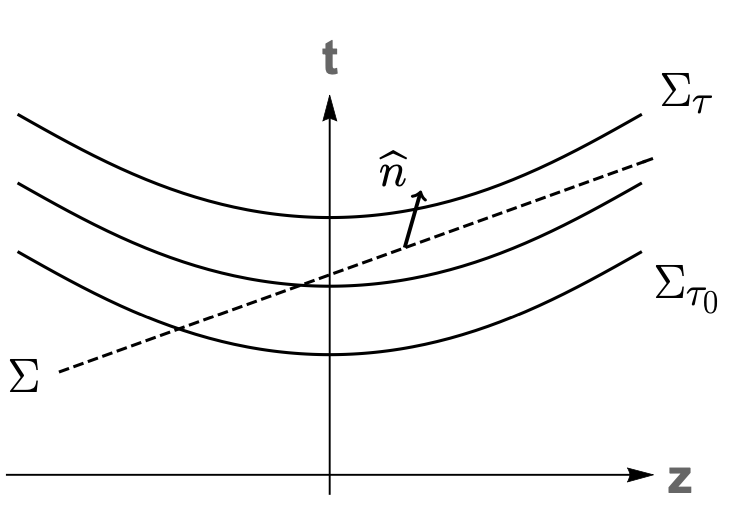
Figure 1: An example of a family of 3D space-like hypersurfaces (solid lines) defining a foliation parametrized by the real variable $\tau$, which is necessary to define local thermodynamic equilibrium. The 3D space-like hypersurface $\Sigma$ does not belong to the foliation.

The dependence of the currents (11) and (13) on the foliation involves a problem in that, if we are to calculate the total entropy by integrating the entropy current (13) on some $\Sigma$ which does not belong to the foliation (see figure 1), the result is in general different from the total entropy which would be obtained from the Von Neumann formula imposing the constraints of local equilibrium (4) over this particular $\Sigma$. In symbols:

$$\int_{\Sigma}{\rm d}\Sigma_{\mu}\;s^{\mu}\neq-\Tr({\widehat{\rho}_{\rm LE}}(\Sigma)\log{\widehat{\rho}_{\rm LE}}(\Sigma))\,,$$ (14)

with equality applying only if $\Sigma$ belongs to the foliation. Such a situation is quite disturbing, as one of the requested features of the entropy current field is to provide the actual value of the total entropy.

To settle the issue, one can define the entropy current more in general as:

$$s^{\mu}=\phi^{\mu}+T^{\mu\nu}\beta_{\nu}-\zeta j^{\mu}-\frac{1}{2}\Omega_{\lambda\nu}{\cal S}^{\mu\lambda\nu}\,,$$ (15)

with (omitting most arguments to make the expression more compact):

$$\phi^{\mu}=\int_{0}^{T}\frac{{\rm d}T^{\prime}}{T^{\prime 2}}\;\left(T^{\mu\nu}[T^{\prime}]u_{\nu}-\mu j^{\mu}[T^{\prime}]-\frac{1}{2}\omega_{\lambda\nu}{\cal S}^{\mu\lambda\nu}[T^{\prime}]\right)\,.$$ (16)

Indeed, in the equations (15) and (16) we have used the actual values of the conserved currents. By doing so, whenever we integrate the currents over some hypersurface $\Sigma$, not necessarily belonging to the original foliation, the result is the same that we would have obtained by enforcing the constraints (4) on $\Sigma$ itself. Since:

$$\int_{\Sigma}{\rm d}\Sigma_{\mu}s^{\mu} =\int_{\Sigma}{\rm d}\Sigma\;n_{\mu}\left(\phi^{\mu}+T^{\mu\nu}\beta_{\nu}-\zeta j^{\mu}-\frac{1}{2}\Omega_{\lambda\nu}{\cal S}^{\mu\lambda\nu}\right)$$

$$=\int_{\Sigma}{\rm d}\Sigma\;n_{\mu}\left(\int_{0}^{T}\frac{{\rm d}T^{\prime}}{T^{\prime 2}}\;\left(T^{\mu\nu}[T^{\prime}]u_{\nu}-\mu j^{\mu}[T^{\prime}]-\frac{1}{2}\omega_{\lambda\nu}{\cal S}^{\mu\lambda\nu}[T^{\prime}]\right)+T^{\mu\nu}\beta_{\nu}-\zeta j^{\mu}-\frac{1}{2}\Omega_{\lambda\nu}{\cal S}^{\mu\lambda\nu}\right)$$

a local equilibrium density operator like in equation (3) can be built on $\Sigma$ by enforcing the constraints (4) therein. Therefore, the above expression becomes, by using the eqs. (9) and (12):

$$\int_{\Sigma}{\rm d}\Sigma\;n_{\mu}\left(\int_{0}^{T}\frac{{\rm d}T^{\prime}}{T^{\prime 2}}\;\left(T^{\mu\nu}_{\rm LE}[T^{\prime}]u_{\nu}-\mu j^{\mu}_{\rm LE}[T^{\prime}]-\frac{1}{2}\omega_{\lambda\nu}{\cal S}^{\mu\lambda\nu}_{\rm LE}[T^{\prime}]\right)+T^{\mu\nu}_{\rm LE}\beta_{\nu}-\zeta j^{\mu}_{\rm LE}-\frac{1}{2}\Omega_{\lambda\nu}{\cal S}^{\mu\lambda\nu}_{\rm LE}\right)$$

$$=-\Tr({\widehat{\rho}_{\rm LE}}(\Sigma)\log{\widehat{\rho}_{\rm LE}}(\Sigma))\,.$$

Similarly, the equation (8) can be extended to a relation which applies to any space-like hypersurface $\Sigma$:

$$\int{\rm d}\Sigma_{\mu}\phi^{\mu}=\log Z_{\rm LE}(\Sigma)+\bra{0}\widehat{\Upsilon}\ket{0}$$ (17)

The two equations (15) and (16) are the final expressions defining the entropy current for a system which is close to local thermodynamic equilibrium. It is worth remarking that those equations imply that the entropy current depends on the actual mean values of the conserved currents ensuing from the quantum field Lagrangian. The question is whether, with the definitions (16) and (15) the thermodynamic potential and entropy current fields are objective, namely independent of a predefined foliation. For this purpose, in the first place the Lagrange multiplier fields $\beta,\zeta,\Omega$ which also appear in those definitions should be independent thereof, a condition which is achieved in relativistic hydrodynamics if they are obtained as solutions of partial differential equations from given initial conditions.

Yet, a complete independence cannot be achieved. Looking carefully at the thermodynamic potential current in the eq. (16), it appears that its definition involves the knowledge of the conserved currents as functionals of the temperature. However, such functionals can be constructed only if the local equilibrium operator is introduced, hence a separation between the local equilibrium term and the dissipative term, which does require the introduction of a foliation. We can signify this limitation by saying that the thermodynamic potential current, and the entropy current as well, can be made quasi-objective. The quasi-objective nature of the entropy current also shows up in the entropy production rate (32), as will be discussed in Section V.

A further issue is that the thermodynamic potential current and the entropy current fields are not unique. It is quite clear that a transformation of the thermodynamic potential current:

$$\phi^{\prime\mu}=\phi^{\mu}+\nabla_{\lambda}A^{\lambda\mu}\,,$$ (18)

where $A^{\lambda\mu}$ is an arbitrary anti-symmetric tensor, implying:

$$s^{\prime\mu}=s^{\mu}+\nabla_{\lambda}A^{\lambda\mu}$$ (19)

will leave the total entropy

$$S=\int_{\Sigma}{\rm d}\Sigma_{\mu}\;s^{\mu}$$

invariant because of the relativistic Stokes theorem, provided that the tensor $A$ fulfills suitable boundary conditions. Therefore, just like $T^{\mu\nu}$ and ${\cal S}^{\mu\lambda\nu}$, the entropy current $s^{\mu}$ is not uniquely defined and can be changed with transformations (19), henceforth defined as entropy-gauge transformations. Such a freedom in defining the entropy current affects the local thermodynamic relations, as we will see. Nevertheless, the divergence of the entropy current is invariant under pseudo-gauge transformations because:

$$\nabla_{\mu}s^{\prime\mu}=\nabla_{\mu}s^{\mu}+\nabla_{\mu}\nabla_{\lambda}A^{\lambda\mu}=\nabla_{\mu}s^{\mu}\,.$$

The entropy production rate will be discussed in Section V.

IV Discussion on local thermodynamic relations

The local thermodynamic relation between proper densities can be obtained by contracting the entropy current with a suitable four-velocity vector. For instance, one can contract the (15) with the four-velocity defined by the direction of $\beta$ that is $u^{\mu}=\beta^{\mu}/\sqrt{\beta^{2}}=T\beta^{\mu}$ :

$$s\equiv s^{\mu}u_{\mu}=\phi\cdot u+\frac{1}{T}\rho-\zeta n-\frac{1}{2}\Omega_{\lambda\nu}u_{\mu}{\cal S}^{\mu\lambda\nu}\equiv\phi\cdot u+\frac{1}{T}\rho-\frac{\mu}{T}n-\frac{1}{2}\Omega_{\lambda\nu}S^{\lambda\nu}\,,$$ (21)

where $\rho=u_{\mu}u_{\nu}T^{\mu\nu}$ and $n=u_{\mu}j^{\mu}$. Defining the pressure as:

$$p\equiv T\phi\cdot u\,,$$

the eq. (21) coincides with the first thermodynamic relation in eq. (2). It should be pointed out though, that only at global equilibrium with $\beta={\rm const}$ this quantity coincides with the hydrostatic pressure, that is the diagonal spatial component of the mean value of the stress-energy tensor (see Appendix A); in all other cases, it does not need to. By contracting the eq. (16) with $u=\beta/\sqrt{\beta^{2}}$ we obtain:

$$\begin{split}p=T\phi\cdot u&=T\int_{0}^{T}\frac{{\rm d}T^{\prime}}{T^{\prime 2}}\;\left(u_{\mu}T^{\mu\nu}[T^{\prime}]u_{\nu}-\mu u_{\mu}j^{\mu}[T^{\prime}]-\frac{1}{2}\omega_{\lambda\nu}u_{\mu}{\cal S}^{\mu\lambda\nu}[T^{\prime}]\right)\\ &=T\int_{0}^{T}\frac{{\rm d}T^{\prime}}{T^{\prime 2}}\;\left(\rho[T^{\prime}]-\mu n_{[}T^{\prime}]-\frac{1}{2}\omega_{\lambda\nu}S^{\lambda\nu}[T^{\prime}]\right)\,,\end{split}$$ (22)

whence the following relation can be readily obtained:

$$\frac{\partial p}{\partial T}\Big{|}_{\mu,\omega}=s$$ (23)

by using the (21). This equation is the first step in proving the second relation (2), but in fact the remaining two partial derivative of the pressure function do not need to coincide with the charge density and the spin density and in general:

$$\frac{\partial p}{\partial\mu}\Big{|}_{T,\omega}\neq n\,,\qquad\qquad\frac{\partial p}{\partial\omega_{\lambda\nu}}\Big{|}_{T,\mu}\neq S^{\lambda\nu}\,.$$

Indeed, for the equality to apply, one would need the following thermodynamic relation to hold:

$$T{\rm d}s={\rm d}\rho-\mu\,{\rm d}n-\frac{1}{2}\omega_{\lambda\nu}{\rm d}S^{\lambda\nu}\,,$$ (24)

and yet this cannot be obtained from the definitions (21) and (16).

Furthermore, the relation (23) is not invariant under entropy-gauge transformations. The thermodynamic potential current can be redefined according to the (18) and, contracting with the four-velocity we get:

$$p^{\prime}=T\phi^{\prime}\cdot u=p+Tu_{\mu}\nabla_{\lambda}A^{\lambda\mu}\,,$$

where the transformed quantities are denoted with a prime. It is then easy to show that:

$$\frac{\partial p^{\prime}}{\partial T}\Big{|}_{\mu\omega}=s^{\prime}+u_{\mu}T\frac{\partial}{\partial T}\nabla_{\lambda}A^{\lambda\mu}\Big{|}_{\mu\omega}\,.$$ (25)

If the second term on the right hand side is non-vanishing, even the relation (23) is broken. An example of an entropy-gauge transformation which breaks the (23) is shown in Appendix C for the global equilibrium with rotation.

In conclusion, the local thermodynamic relations (2) are not fully appropriate in the derivation of the divergence of the entropy current. On one hand, it turns out that the differential relation in (2) cannot be proved in general and on the other hand, perhaps most importantly, because they are both non-invariant under entropy-gauge transformations.

V Entropy production rate

The entropy production rate, which is important to obtain the constitutive equations of relativistic hydrodynamics, is determined by taking the divergence of the equation (15). By using the continuity equations of the stress-energy tensor, the number current and the spin tensor, that is:

$$\nabla_{\mu}T^{\mu\nu}=0\,,\qquad\nabla_{\mu}j^{\mu}=0\,,\qquad\nabla_{\mu}{\cal S}^{\mu\lambda\nu}=T^{\nu\lambda}-T^{\lambda\nu}\,,$$ (26)

we obtain:

$$\begin{split}\nabla_{\mu}s^{\mu}&=\nabla_{\mu}\phi^{\mu}+T^{\mu\nu}\nabla_{\mu}\beta_{\nu}-j^{\mu}\nabla_{\mu}\zeta-\frac{1}{2}{\cal S}^{\mu\lambda\nu}\nabla_{\mu}\Omega_{\lambda\nu}-\frac{1}{2}\Omega_{\lambda\nu}\nabla_{\mu}{\cal S}^{\mu\lambda\nu}\\ &=\nabla_{\mu}\phi^{\mu}+T_{S}^{\mu\nu}\xi_{\mu\nu}-j^{\mu}\nabla_{\mu}\zeta+T_{A}^{\mu\nu}(\Omega_{\mu\nu}-\varpi_{\mu\nu})-\frac{1}{2}{\cal S}^{\mu\lambda\nu}\nabla_{\mu}\Omega_{\lambda\nu}\,,\end{split}$$ (27)

where $T_{S}$ and $T_{A}$ are the symmetric and anti-symmetric parts of the stress-energy tensor and

$$\xi_{\mu\nu}=\frac{1}{2}\left(\nabla_{\mu}\beta_{\nu}+\nabla_{\nu}\beta_{\mu}\right)\,,\qquad\varpi_{\mu\nu}=\frac{1}{2}\left(\nabla_{\nu}\beta_{\mu}-\nabla_{\mu}\beta_{\nu}\right)$$

are the thermal shear and thermal vorticity tensor respectively.

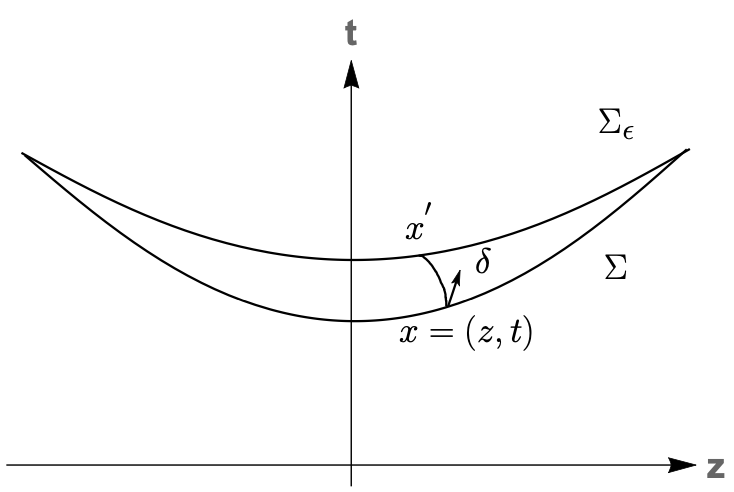
Figure 2: The hypersurface $\Sigma$ is mapped to $\Sigma_{\epsilon}$ by an infinitesimal diffeomorphism $\epsilon$. The vector field $\delta(x)$ is defined as ${\rm d}x^{\prime}(x,\epsilon)/{\rm d}\epsilon|_{\epsilon=0}$.

The next step, as it appears from the equation (27), is the calculation of the divergence of the thermodynamic potential current, $\nabla_{\mu}\phi^{\mu}$. To derive it, it is convenient to study the change of $\log Z_{\rm LE}$ under an infinitesimal change of the integration 3D hypersurface (see figure 2). An infinitesimal change of hypersurface may be seen, in simple terms, as the result of locally moving every point $x\in\Sigma$ to a point $x^{\prime}(x,\epsilon)\in\Sigma_{\epsilon}$, $\epsilon$ being a finite real parameter. Setting $x^{\prime}(x,0)=x$, we define:

$$\frac{{\rm d}x^{\prime\mu}(x,\epsilon)}{{\rm d}\epsilon}\Big{|}_{\epsilon=0}=\delta^{\mu}(x)\,.$$

For a small $\epsilon$, the vector field $\delta$ loosely represents the direction in which the hypersurface is locally modified and the parameter $\epsilon$ describes how far along the vector field $\delta$ we move the hypersurface. Formally, these definitions are those of a one-parameter group of diffeomorphisms, which are a prerequisite to define the Lie derivative. For the special case of the integration of a vector field $V^{\mu}$ over a 3D-hypersurface, one has (see Appendix B):

$$\lim_{\epsilon\to\ 0}\frac{1}{\epsilon}\left(\int_{\Sigma_{\epsilon}}{\rm d}\Sigma_{\mu}V^{\mu}-\int_{\Sigma}{\rm d}\Sigma_{\mu}\,V^{\mu}\right)=\int_{\partial\Sigma}{\rm d}\tilde{S}_{\mu\nu}\,\delta^{\mu}V^{\nu}+\int_{\Sigma}{\rm d}\Sigma\cdot\delta\,\nabla_{\mu}V^{\mu}\,,$$ (28)

where $\partial\Sigma$ is the 2-D boundary surface. We can apply this equation to the (17) to obtain the infinitesimal change of $\log Z_{\rm LE}$ by a change of the hypersurface:

$$\lim_{\epsilon\to\ 0}\frac{1}{\epsilon}\left[\log Z_{\rm LE}(\Sigma_{\epsilon})-\log Z_{\rm LE}(\Sigma)\right]=\int_{\Sigma}{\rm d}\Sigma\cdot\delta\,\nabla_{\mu}\left(\phi^{\mu}-\bra{0}{\widehat{T}}^{\mu\nu}\beta_{\nu}-\zeta{\widehat{j}}^{\mu}-\frac{1}{2}\Omega_{\lambda\nu}{\widehat{\cal S}}^{\mu\lambda\nu}\ket{0}\right)$$

$$=\int_{\Sigma}{\rm d}\Sigma\cdot\delta\,\nabla_{\mu}\phi^{\mu}-\int_{\Sigma}{\rm d}\Sigma\cdot\delta\,\bra{0}{\widehat{T}}_{S}^{\mu\nu}\xi_{\mu\nu}-{\widehat{j}}^{\mu}\nabla_{\mu}\zeta+{\widehat{T}}_{A}^{\mu\nu}(\Omega_{\mu\nu}-\varpi_{\mu\nu})-\frac{1}{2}{\widehat{\cal S}}^{\mu\lambda\nu}\nabla_{\mu}\Omega_{\lambda\nu}\ket{0}\,,$$ (29)

where, in the last step, we have used the continuity equations (26), holding at operator level. On the other hand, the logarithm of the partition function can be calculated by means of its definition as a trace. For an infinitesimal $\epsilon$ one has:

$$Z_{\rm LE}(\Sigma_{\epsilon})=\Tr\left(\exp\left[-\int_{\Sigma_{\epsilon}}{\rm d}\Sigma_{\mu}\left({\widehat{T}}^{\mu\nu}\beta_{\nu}-\zeta{\widehat{j}}^{\mu}-\frac{1}{2}\Omega_{\lambda\nu}{\widehat{\cal S}}^{\mu\lambda\nu}\right)\right]\right)$$

$$\simeq\Tr\left(\exp\left[-\int_{\Sigma}{\rm d}\Sigma_{\mu}\left({\widehat{T}}^{\mu\nu}\beta_{\nu}-\zeta{\widehat{j}}^{\mu}-\frac{1}{2}\Omega_{\lambda\nu}{\widehat{\cal S}}^{\mu\lambda\nu}\right)-\epsilon\int_{\Sigma}{\rm d}\Sigma\cdot\delta\nabla_{\mu}\left({\widehat{T}}^{\mu\nu}\beta_{\nu}-\zeta{\widehat{j}}^{\mu}-\frac{1}{2}\Omega_{\lambda\nu}{\widehat{\cal S}}^{\mu\lambda\nu}\right)\right]\right)$$

$$=\Tr\left(\exp\left[-\int_{\Sigma}{\rm d}\Sigma_{\mu}\left({\widehat{T}}^{\mu\nu}\beta_{\nu}-\zeta{\widehat{j}}^{\mu}-\frac{1}{2}\Omega_{\lambda\nu}{\widehat{\cal S}}^{\mu\lambda\nu}\right)\right.\right.$$

$$-\left.\left.\epsilon\int_{\Sigma}{\rm d}\Sigma\cdot\delta\;\left({\widehat{T}}_{S}^{\mu\nu}\xi_{\mu\nu}-{\widehat{j}}^{\mu}\nabla_{\mu}\zeta+{\widehat{T}}_{A}^{\mu\nu}(\Omega_{\mu\nu}-\varpi_{\mu\nu})-\frac{1}{2}{\widehat{\cal S}}^{\mu\lambda\nu}\nabla_{\mu}\Omega_{\lambda\nu}\right)\right]\right)\,,$$

where we have used the equation (28) - assuming that the boundary term vanishes - and, again, the continuity equations (26) at operator level. By expanding the trace in the small parameter $\epsilon$, and keeping in mind the equation (3), we obtain:

$$Z_{\rm LE}(\Sigma_{\epsilon}) \simeq Z_{\rm LE}(\Sigma)-\epsilon Z_{\rm LE}(\Sigma)$$

$$\times\int_{\Sigma}{\rm d}\Sigma\cdot\delta\;\left(\Tr({\widehat{\rho}_{\rm LE}}{\widehat{T}}_{S}^{\mu\nu})\xi_{\mu\nu}-\Tr({\widehat{\rho}_{\rm LE}}{\widehat{j}}^{\mu})\nabla_{\mu}\zeta+\Tr({\widehat{\rho}_{\rm LE}}{\widehat{T}}_{A}^{\mu\nu})(\Omega_{\mu\nu}-\varpi_{\mu\nu})-\frac{1}{2}\Tr({\widehat{\rho}_{\rm LE}}{\widehat{\cal S}}^{\mu\lambda\nu})\nabla_{\mu}\Omega_{\lambda\nu}\right)\,,$$

whence:

$$\lim_{\epsilon\to\ 0}\frac{1}{\epsilon}\left[\log Z_{\rm LE}(\Sigma_{\epsilon})-\log Z_{\rm LE}(\Sigma)\right]$$ (30)

$$=-\int_{\Sigma}{\rm d}\Sigma\cdot\delta\;\left(\Tr({\widehat{\rho}_{\rm LE}}{\widehat{T}}_{S}^{\mu\nu})\xi_{\mu\nu}-\Tr({\widehat{\rho}_{\rm LE}}{\widehat{j}}^{\mu})\nabla_{\mu}\zeta+\Tr({\widehat{\rho}_{\rm LE}}{\widehat{T}}_{A}^{\mu\nu})(\Omega_{\mu\nu}-\varpi_{\mu\nu})-\frac{1}{2}\Tr({\widehat{\rho}_{\rm LE}}{\widehat{\cal S}}^{\mu\lambda\nu})\nabla_{\mu}\Omega_{\lambda\nu}\right)\,.$$

Therefore, by comparing the equation (V) with the equation (30), taking into account that both $\Sigma$ and the field $\delta$ are arbitrary, we can infer that:

$$\nabla_{\mu}\phi^{\mu} =-\left[\left(\Tr({\widehat{\rho}_{\rm LE}}{\widehat{T}}_{S}^{\mu\nu})-\bra{0}{\widehat{T}}_{S}^{\mu\nu}\ket{0}\right)\xi_{\mu\nu}-\left(\Tr({\widehat{\rho}_{\rm LE}}{\widehat{j}}^{\mu})-\bra{0}{\widehat{j}}^{\mu}\ket{0}\right)\nabla_{\mu}\zeta\right.$$

$$+\left.\left(\Tr({\widehat{\rho}_{\rm LE}}{\widehat{T}}_{A}^{\mu\nu})-\bra{0}{\widehat{T}}_{A}^{\mu\nu}\ket{0}\right)(\Omega_{\mu\nu}-\varpi_{\mu\nu})-\frac{1}{2}\left(\Tr({\widehat{\rho}_{\rm LE}}{\widehat{\cal S}}^{\mu\lambda\nu})-\bra{0}{\widehat{\cal S}}^{\mu,\lambda\nu}\ket{0}\right)\nabla_{\mu}\Omega_{\lambda\nu}\right]$$

$$=-\left(T^{\mu\nu}_{S\rm(LE)}\xi_{\mu\nu}-j^{\mu}_{\rm LE}\nabla_{\mu}\zeta+T^{\mu\nu}_{A\rm(LE)}(\Omega_{\mu\nu}-\varpi_{\mu\nu})-\frac{1}{2}{\cal S}^{\mu\lambda\nu}_{\rm LE}\nabla_{\mu}\Omega_{\lambda\nu}\right)\,,$$ (31)

where, in the last step, we have used the definition of local equilibrium values.

Now, substituting back the eq. (V) into the eq. (27), we obtain the evolution of entropy current:

$$\nabla_{\mu}s^{\mu}=\left(T_{S}^{\mu\nu}-T^{\mu\nu}_{S(\rm LE)}\right)\xi_{\mu\nu}-\left(j^{\mu}-j^{\mu}_{\rm LE}\right)\nabla_{\mu}\zeta+\left(T^{\mu\nu}_{A}-T^{\mu\nu}_{A(\rm LE)}\right)(\Omega_{\mu\nu}-\varpi_{\mu\nu})-\frac{1}{2}\left({\cal S}^{\mu\lambda\nu}-{\cal S}^{\mu\lambda\nu}_{\rm LE}\right)\nabla_{\mu}\Omega_{\lambda\nu}\,.$$ (32)

The equation (32) is the main result of this work and it is the starting point to derive the constitutive equations of dissipative spin hydrodynamics, which relate the anti-symmetric part of the stress-energy tensor and the spin tensor to the gradients of the spin potential and the difference between spin potential and thermal vorticity, besides the (thermal) shear tensor and the gradient of $\zeta=\mu/T$. In the above form, it is in fact a generalization of the one found by Van Weert and Zubarev [24, 25], with the addition of the last two terms involving spin tensor and the spin potential. We stress that the formula (32) is exact and not an approximation at some order of a gradient expansion. Indeed, with respect to all previous assessments of dissipative spin hydrodynamics based on different approaches  [7, 8, 9, 10, 11, 12, 13], a novel feature is apparently the simultaneous appearance of the last two terms of the right hand side. While the last term is neglected in almost all derivations, it was actually obtained in ref. [10]. However, it should be pointed out that some terms in previous derivations may have been omitted because of a gradient power counting method. A complete analysis of the constitutive equations implied by the (32) will be presented in a forthcoming study.

VI Discussion and conclusions

The formula (32) shows that entropy production rate, in general, is non-vanishing whenever there is a difference between the actual value of the conserved (or conserved-related) currents and the corresponding values at local thermodynamic equilibrium, such as $T_{S(\rm LE)}$, $j_{\rm LE}$, etc. As we have emphasized in this paper, local equilibrium depends on the choice of a family of 3D space-like hypersurfaces, i.e. a foliation. In relativistic hydrodynamics, this freedom ultimately corresponds to the choice of a four-velocity vector, so-called hydrodynamic frame. The dependence on the foliation shows up in the divergence of the entropy current (32), which is manifestly dependent on local equilibrium values (see the discussion at the end of Section III).

We emphasize that the formula (32) is exact, not an approximation at some order of a gradient expansion. In other words, fixing the order in a gradient expansion of hydrodynamic quantities is not required to obtain it. However, for future work, once constitutive equations are determined, a gradient ordering can be made based on the involved scales in the physical problem.

In conclusion, in this work we have employed a quantum-statistical approach to derive the entropy current and entropy production rate without assuming the traditional local thermodynamic relations (2). In fact, we have shown that the local thermodynamic relations do not hold in general and that they are also non-invariant under allowed transformations of the entropy current, that we have defined as entropy-gauge transformations. We have obtained an expression of the entropy production rate (32) which extends to spin hydrodynamics previous expression obtained in refs. [24, 25]. This form is especially well-suited to derive the constitutive equations of dissipative spin hydrodynamics, what will be the subject of a forthcoming work.

Appendix A Thermodynamic potential current at homogeneous global equilibrium

Homogeneous global equilibrium is defined by the condition $\beta=\mbox{const}$ i.e. vanishing thermal vorticity in the equation (7). Plugging this form in the equation (3), the density operator takes on the familiar form (for simplicity, we assume there are no charges in the system):

$${\widehat{\rho}}_{\rm GE}=\frac{1}{Z}\exp\left[-\beta\cdot{\widehat{P}}\right]\,.$$ (33)

Due to the symmetries of the above operator, the mean value of the stress-energy tensor operator has the ideal form:

$$T^{\mu\nu}=\Tr({\widehat{\rho}}_{\rm GE}{\widehat{T}}^{\mu\nu})-\bra{0}{\widehat{T}}^{\mu\nu}\ket{0}=(\rho+p)u^{\mu}u^{\nu}-pg^{\mu\nu}\,,$$ (34)

where $u\equiv\beta/{\sqrt{\beta^{2}}}$. According to eq. (16), the thermodynamic potential current is:

$$\phi^{\mu}=\int_{0}^{T}\frac{{\rm d}T^{\prime}}{T^{\prime 2}}\;T^{\mu\nu}[T^{\prime}]u_{\nu}=\int_{0}^{T}\frac{{\rm d}T^{\prime}}{T^{\prime 2}}\;\rho[T^{\prime}]u^{\mu}\,,$$ (35)

where $T=1/\sqrt{\beta^{2}}$. The above expression confirms the expectation that, at the homogeneous global equilibrium, any vector field should be parallel to $\beta$ with a coefficient depending on $\beta^{2}$ or, equivalently, the temperature $T$. Therefore:

$$\phi^{\mu}=\beta^{\mu}\phi(\beta^{2})$$ (36)

and the goal is now to show that such scalar coefficient $\phi(\beta^{2})$ is just the pressure, as defined by the equation (34).

By taking the derivative with respect to $\beta$ of the partition function, we have:

$$-\frac{\partial\log Z}{\partial\beta_{\nu}}=\Tr({\widehat{\rho}}_{\rm GE}{\widehat{P}}^{\nu})=\int_{\Sigma}{\rm d}\Sigma_{\mu}\;\Tr({\widehat{\rho}}_{\rm GE}{\widehat{T}}^{\mu\nu})\,.$$ (37)

Since:

$$\log Z=\int{\rm d}\Sigma_{\mu}\;\phi^{\mu}-\beta_{\nu}\bra{0}{\widehat{P}}^{\nu}\ket{0}$$

from the (8), from the (37) we can obtain the following equality

$$\int_{\Sigma}{\rm d}\Sigma_{\mu}\left(\frac{\partial\phi^{\mu}}{\partial\beta_{\nu}}\right)=-\int_{\Sigma}{\rm d}\Sigma_{\mu}T^{\mu\nu}\,,$$ (38)

where we have used the (34). Since the integration hypersurface $\Sigma$ is arbitrary, being at global equilibrium, we can infer the following relation:

$$T^{\mu\nu}=-\frac{\partial\phi^{\mu}}{\partial\beta_{\nu}}+\partial_{\lambda}A^{\lambda\mu\nu}\,,$$

where the rank 3 tensor $A^{\lambda\mu\nu}$ is anti-symmetric in the indices $\lambda\mu$. Such a gradient term is allowed by the Stokes theorem in Minkowski space-time if suitable boundary conditions are fulfilled. Yet, since the equilibrium is homogeneous, it must vanish due to traslational invariance as all mean values ought to be constant and uniform. This implies that, by using the equation (36):

$$T^{\mu\nu}=-\frac{\partial\phi^{\mu}}{\partial\beta_{\nu}}=-\frac{\partial}{\partial\beta_{\nu}}\phi\beta^{\mu}=-\phi g^{\mu\nu}+T\frac{\partial\phi}{\partial T}u^{\mu}u^{\nu}\,.$$ (39)

We can now compare (34) with (39) and infer that $\phi=p$ and consequently $\phi^{\mu}=p\beta^{\mu}$. By plugging the latter equation in the (35) and taking the derivative with respect to $T$ we obtain:

$$T\frac{\partial p}{\partial T}=\rho+p\,,$$

which makes also the second term on the right hand side of equation (39) consistent with the identification $\phi=p$.

Appendix B Lie derivatives and integration

Suppose we have a one-parameter group of diffeomorphisms $x^{\prime}(x,\epsilon)$ with $\epsilon$ a real number. Let $\omega$ be a rank 3 differential form which is to be integrated over a 3D hypersurface embedded in the 4D space-time. We denote with $\omega^{\prime}_{\epsilon}$ the differential form which is obtained from $\omega$ through the diffeomorphism, that is:

$$\omega^{\prime}_{\epsilon}(x)_{\mu_{1}\mu_{2}\mu_{3}}=J_{\mu_{1}}^{\nu_{1}}J_{\mu_{2}}^{\nu_{2}}J_{\mu_{3}}^{\nu_{3}}\;\omega(x^{\prime}(x,\epsilon))_{\nu_{1},\nu_{2},\nu_{3}}$$

where $J_{\mu}^{\nu}=\partial x^{\prime}(x,\epsilon)^{\nu}/\partial x^{\mu}$ is the jacobian matrix element of the diffeomorphism. Let $\Sigma_{\epsilon}$ be the image of the hypersurface $\Sigma$ through the diffeomorphism. Then we have:

$$\int_{\Sigma_{\epsilon}}\omega=\int_{\Sigma}\omega^{\prime}_{\epsilon}$$

whence:

$$\lim_{\epsilon\to 0}\frac{1}{\epsilon}\left(\int_{\Sigma_{\epsilon}}\omega(x)-\int_{\Sigma}\omega(x)\right)=\lim_{\epsilon\to 0}\frac{1}{\epsilon}\int_{\Sigma}\omega^{\prime}_{\epsilon}(x)-\omega(x)=\int_{\Sigma}{\cal L}_{\delta}(\omega(x))\,,$$

where ${\cal L}_{\delta}$ stands for the Lie derivative along the vector field $\delta(x)={\rm d}x^{\prime}(x,\epsilon)/{\rm d}\epsilon|_{\epsilon=0}$.

The so-called Cartan magic formula can now be used in the last expression, leading to:

$$\int_{\Sigma}{\cal L}_{\delta}(\omega)=\int_{\Sigma}i_{\delta}{\rm d}\omega+{\rm d}(i_{\delta}\omega)=\int_{\Sigma}i_{\delta}{\rm d}\omega+\int_{\partial\Sigma}i_{\delta}\omega\,,$$ (40)

where $i_{\delta}$ stands for the interior product of the form with the vector field $\delta$ and ${\rm d}$ stands for the exterior derivative. The second term on the right hand side of (40) is an integral of an exterior derivative and it has been turned into a 2D boundary integral of $i_{\delta}\omega$ by using the generalized Stokes theorem for differential forms.

We can apply the above formulae to the differential form which is the dual of a vector field $V$ in a 4D space-time, namely:

$$\omega_{\mu\nu\rho}=\frac{1}{6}E_{\mu\nu\rho\sigma}V^{\sigma}=\frac{1}{6}\sqrt{|g|}\epsilon_{\mu\nu\rho\sigma}V^{\sigma}\,.$$ (41)

With this form, it can be shown that:

$$\int_{\Sigma}\omega(x)=\int_{\Sigma}{\rm d}\Sigma_{\mu}V^{\mu}\,.$$ (42)

The exterior derivative can be readily worked out by using the definition:

$$({\rm d}\omega)_{\lambda\mu\nu\rho}=-\frac{1}{24}E_{\lambda\mu\nu\rho}\nabla\cdot V\,,$$

which leads, by using the definition of interior product, to:

$$(i_{\delta}{\rm d}\omega)_{\mu\nu\rho}=\frac{1}{6}E_{\mu\nu\rho\sigma}\delta^{\sigma}\nabla\cdot V\,.$$

Therefore, by using the above expression and the (42) we get:

$$\int_{\Sigma}i_{\delta}{\rm d}\omega=\int_{\Sigma}{\rm d}\Sigma_{\mu}\,\delta^{\mu}\nabla\cdot V\,.$$

The second integral in the (40) can be similarly worked out and one eventually obtains the equation (28).

Appendix C Non-invariance of the local thermodynamic relations: an example

We are going to show that the local thermodynamic relation (23) is not invariant under entropy-gauge transformation (18), namely that the equation (25) applies with a non-trivial second term in the right hand side.

We consider, as specific example, global equilibrium with non-vanishing thermal vorticity in the equation (7). Let:

$$A^{\lambda\mu}=f(\kappa^{2})\varpi^{\lambda\mu}\,,$$

where $\kappa^{\mu}=\varpi^{\mu\nu}\beta_{\nu}$ and $f(\kappa^{2})=g(\kappa^{2})/\kappa^{2}$ with $g(\kappa^{2})$ an adimensional differentiable function (this form of $f(\kappa^{2})$ ensures that $A^{\lambda\mu}$ has the correct dimension for the entropy gauge transformation (18)). One has, in Cartesian coordinates:

$$\nabla_{\lambda}A^{\lambda\mu}=\partial_{\lambda}A^{\lambda\mu}=f^{\prime}(\kappa^{2})\varpi^{\lambda\mu}\partial_{\lambda}\kappa^{2}=f^{\prime}(\kappa^{2})\varpi^{\lambda\mu}2\kappa^{\nu}\partial_{\lambda}\kappa_{\nu}=f^{\prime}(\kappa^{2})\varpi^{\lambda\mu}2\kappa^{\nu}\partial_{\lambda}(\varpi_{\nu\rho}\beta^{\rho})=f^{\prime}(\kappa^{2})\varpi^{\lambda\mu}2\kappa^{\nu}\varpi_{\nu\rho}\varpi^{\rho}_{\;\lambda}\,,$$

where, in the last step, we have used the relation $\varpi_{\mu\nu}=\partial_{\nu}\beta_{\mu}$ which applies at global equilibrium where $\partial_{\mu}\beta_{\nu}+\partial_{\nu}\beta_{\mu}=0$.

Now let $\gamma^{\rho}=\varpi^{\rho\nu}\kappa_{\nu}$ so that:

$$\partial_{\lambda}A^{\lambda\mu}=-2f^{\prime}(\kappa^{2})\gamma^{\rho}\varpi_{\rho\lambda}\varpi^{\lambda\mu}\,.$$ (43)

Contracting the equation (43) with $u_{\mu}$ we get:

$$u_{\mu}\partial_{\lambda}A^{\lambda\mu}=T\beta_{\mu}\partial_{\lambda}A^{\lambda\mu}=-2f^{\prime}(\kappa^{2})T\gamma^{\rho}\varpi_{\rho\lambda}\varpi^{\lambda\mu}\beta_{\mu}=-2f^{\prime}(\kappa^{2})T\gamma^{\rho}\varpi_{\rho\lambda}\kappa^{\lambda}=-2f^{\prime}(\kappa^{2})T\gamma^{2}\,.$$ (44)

The derivative in (25) must be taken by keeping $\omega=T\varpi$ constant. Therefore, being:

$$\kappa^{\mu}=\varpi^{\mu\nu}\beta_{\nu}=\frac{1}{T^{2}}\omega^{\mu\nu}u_{\nu}\,,\qquad\qquad\gamma^{\rho}=\varpi^{\rho\nu}\kappa_{\nu}=\frac{1}{T^{3}}\omega^{\rho\nu}\omega_{\nu\alpha}u^{\alpha}\,,$$

and choosing $g(\kappa^{2})=1$, we have that the expression in the equation (44) is proportional to $T^{3}$,

$$T\frac{\partial}{\partial T}\left(u_{\mu}\partial_{\lambda}A^{\lambda\mu}\right)=T\frac{2}{(\kappa^{2})^{2}}\gamma^{2}\,,$$ (45)

which is non-vanishing. Therefore, using the (45) in the equation (25) we get:

$$\frac{\partial p^{\prime}}{\partial T}\Big{|}_{\mu\omega}=s^{\prime}+T\frac{2}{(\kappa^{2})^{2}}\gamma^{2}\,,$$

which proves the non-invariance of the local thermodynamic relation.

References

- [1] STAR Collaboration, L. Adamczyk et al., “Global hyperon polarization in nuclear collisions: evidence for the most vortical fluid,” Nature 548 (2017) 62–65, arXiv:1701.06657 [nucl-ex].
- [2] STAR Collaboration, T. Niida, “Global and local polarization of hyperons in Au+Au collisions at 200 GeV from STAR,” Nucl. Phys. A 982 (2019) 511–514, arXiv:1808.10482 [nucl-ex].
- [3] F. Becattini, “Hydrodynamics of fluids with spin,” Phys. Part. Nucl. Lett. 8 (2011) 801–804.
- [4] W. Florkowski, B. Friman, A. Jaiswal, and E. Speranza, “Relativistic fluid dynamics with spin,” Phys. Rev. C 97 no. 4, (2018) 041901, arXiv:1705.00587 [nucl-th].
- [5] W. Florkowski, A. Kumar, and R. Ryblewski, “Relativistic hydrodynamics for spin-polarized fluids,” Prog. Part. Nucl. Phys. 108 (2019) 103709, arXiv:1811.04409 [nucl-th].
- [6] D. Montenegro, L. Tinti, and G. Torrieri, “The ideal relativistic fluid limit for a medium with polarization,” Phys. Rev. D96 no. 5, (2017) 056012, arXiv:1701.08263 [hep-th].
- [7] K. Hattori, M. Hongo, X.-G. Huang, M. Matsuo, and H. Taya, “Fate of spin polarization in a relativistic fluid: An entropy-current analysis,” Phys. Lett. B 795 (2019) 100–106, arXiv:1901.06615 [hep-th].
- [8] K. Fukushima and S. Pu, “Spin hydrodynamics and symmetric energy-momentum tensors – A current induced by the spin vorticity –,” Phys. Lett. B 817 (2021) 136346, arXiv:2010.01608 [hep-th].
- [9] A. Daher, A. Das, W. Florkowski, and R. Ryblewski, “Canonical and phenomenological formulations of spin hydrodynamics,” Phys. Rev. C 108 no. 2, (2023) 024902, arXiv:2202.12609 [nucl-th].
- [10] D. She, A. Huang, D. Hou, and J. Liao, “Relativistic viscous hydrodynamics with angular momentum,” Sci. Bull. 67 (2022) 2265–2268, arXiv:2105.04060 [nucl-th].
- [11] M. Hongo, X.-G. Huang, M. Kaminski, M. Stephanov, and H.-U. Yee, “Relativistic spin hydrodynamics with torsion and linear response theory for spin relaxation,” JHEP 11 (2021) 150, arXiv:2107.14231 [hep-th].
- [12] A. D. Gallegos, U. Gürsoy, and A. Yarom, “Hydrodynamics of spin currents,” SciPost Phys. 11 (2021) 041, arXiv:2101.04759 [hep-th].
- [13] A. D. Gallegos, U. Gursoy, and A. Yarom, “Hydrodynamics, spin currents and torsion,” arXiv:2203.05044 [hep-th].
- [14] H.-H. Peng, J.-J. Zhang, X.-L. Sheng, and Q. Wang, “Ideal Spin Hydrodynamics from the Wigner Function Approach,” Chin. Phys. Lett. 38 no. 11, (2021) 116701, arXiv:2107.00448 [hep-th].
- [15] Z. Cao, K. Hattori, M. Hongo, X.-G. Huang, and H. Taya, “Gyrohydrodynamics: Relativistic spinful fluid with strong vorticity,” PTEP 2022 no. 7, (2022) 071D01, arXiv:2205.08051 [hep-th].
- [16] N. Weickgenannt, D. Wagner, E. Speranza, and D. H. Rischke, “Relativistic second-order dissipative spin hydrodynamics from the method of moments,” Phys. Rev. D 106 no. 9, (2022) 096014, arXiv:2203.04766 [nucl-th].
- [17] N. Weickgenannt, D. Wagner, E. Speranza, and D. H. Rischke, “Relativistic dissipative spin hydrodynamics from kinetic theory with a nonlocal collision term,” Phys. Rev. D 106 no. 9, (2022) L091901, arXiv:2208.01955 [nucl-th].
- [18] R. Biswas, A. Daher, A. Das, W. Florkowski, and R. Ryblewski, “Relativistic second-order spin hydrodynamics: An entropy-current analysis,” Phys. Rev. D 108 no. 1, (2023) 014024, arXiv:2304.01009 [nucl-th].
- [19] X.-Q. Xie, D.-L. Wang, C. Yang, and S. Pu, “Causality and stability analysis for the minimal causal spin hydrodynamics,” arXiv:2306.13880 [hep-ph].
- [20] F. W. Hehl, “On the Energy Tensor of Spinning Massive Matter in Classical Field Theory and General Relativity,” Rept. Math. Phys. 9 (1976) 55–82.
- [21] F. Becattini and L. Tinti, “Thermodynamical inequivalence of quantum stress-energy and spin tensors,” Phys. Rev. D 84 (2011) 025013, arXiv:1101.5251 [hep-th].
- [22] F. Becattini, W. Florkowski, and E. Speranza, “Spin tensor and its role in non-equilibrium thermodynamics,” Phys. Lett. B789 (2019) 419–425, arXiv:1807.10994 [hep-th].
- [23] M. Buzzegoli, “Pseudogauge dependence of the spin polarization and of the axial vortical effect,” Phys. Rev. C 105 no. 4, (2022) 044907, arXiv:2109.12084 [nucl-th].
- [24] C. van Weert, “Maximum entropy principle and relativistic hydrodynamics,” Annals of Physics, Volume 140, Issue 1,1982 .
- [25] D. N. Zubarev, A. N. Prozorkevich, and S. A. Smolyanskii, “Derivation of nonlinear generalized equations of quantum relativistic hydrodynamics,” Theor. Math. Phys. 40, 821–831 (1979) .
- [26] F. Becattini, L. Bucciantini, E. Grossi, and L. Tinti, “Local thermodynamical equilibrium and the beta frame for a quantum relativistic fluid,” Eur. Phys. J. C 75 no. 5, (2015) 191, arXiv:1403.6265 [hep-th].
- [27] F. Becattini and D. Rindori, “Extensivity, entropy current, area law and Unruh effect,” Phys. Rev. D 99 no. 12, (2019) 125011, arXiv:1903.05422 [hep-th].