A New Framework to Estimate Return on Investment for Player Salaries in the National Basketball Association

Abstract

The National Basketball Association (NBA) imposes a player salary cap. It is therefore useful to develop tools to measure the relative realized return of a player’s salary given their on court performance. Very few such studies exist, however. We thus present the first known framework to estimate a return on investment (ROI) for NBA player contracts. The framework operates in five parts. First, we decide on a measurement time horizon, such as the standard 82-game NBA regular season. Second, we propose the novel game contribution percentage (GCP) measure, which is a single game summary statistic that sums to unity for each competing team and is comprised of traditional, playtype, hustle, box outs, defensive, tracking, and rebounding per game NBA statistics. Next, we estimate the single game value (SGV) of each regular season NBA game using a standard currency conversion calculation. Fourth, we multiply the SGV by the vector of realized GCPs to obtain a series of realized per-player single season cash flows. Finally, we use the player salary as an initial investment to perform the traditional ROI calculation. We illustrate our framework by compiling a novel, sharable dataset of per game GCP statistics and salaries for the 2022-2023 NBA regular season. Using only total GCP, we find the top five performers to be Domantas Sabonis, Nikola Jokić, Joel Embiid, Luka Dončić, and Bam Adebayo. With player salaries, however, the top five ROI performers become Tre Jones, Kevon Harris, Nick Richards, Ayo Dosunmu, and Max Strus. A scatter plot of ROI by salary for all players is presented. Notably, missed games are treated as defaults because GCP is a per game metric. This allows for break-even calculations between high-performing players with frequent missed games and average performers with few missed games, which we demonstrate with a comparison of the 2023 NBA regular seasons of Anthony Davis and Brook Lopez. We conclude by suggesting uses of our framework, discussing its flexibility through customization, and outlining potential future improvements.

Keywords: Load management, internal rate of return, IRR, most valuable player, NBA economics, NBA finance, NBA profitability, PVGCP

1 Introduction

On December 20, 2022, the Phoenix Suns of the National Basketball Association (NBA) in combination with the Phoenix Mercury of the Women’s National Basketball Association were purchased at a valuation price of $4 billion (Wojnarowski, 2022); the NBA is big business. As in any financial operation, it is of great interest to assess performance for the purposes of allocating returns to investors or other parties with pecuniary interests. Among the many financial interests of NBA teams, such as ticket sales, television revenue, and merchandise sales, there is the obvious consideration of compensating the players that make up each team’s roster. This task is made complicated by a myriad of reasons, not the least of which is that the NBA operates within a framework designed to restrict a free market. Indeed, a crucial component of the competitive parameters of the NBA is a salary cap, which set a minimum total salary of $111.290 million and a maximum total salary of $123.655 million per team for the 2022-2023 NBA season (National Basketball Association, 2022), subject to numerous additional restrictions (National Basketball Association, 2018). Thus, how to effectively allocate this fixed total salary to on court personnel is a crucial component of a team’s on court success.

It is natural, then, to suppose there exists a great number of studies that consider both on court performance and salary simultaneously to arrive at methods to measure realized return on investment (ROI) or the internal rate of return (IRR) of a player’s contract in view of said player’s on court performance. A survey of related studies indicates that this is not the case, however. Idson and Kahane (2000) attempt to derive the determinants of a player’s salary in the National Hockey League with a model that incorporates the performance of teammates. We consider the NBA, however, and our methodology differs considerably (see Section 2). Berri et al. (2005) identify the importance of height in the NBA and juxtaposes it against population height distributions to explain competitive imbalances observed in the NBA. Such imbalances are thought to negatively impact economic outcomes of sports leagues (Berri et al., 2005). While financial considerations enter into the analysis of Berri et al. (2005), it does not concern the ROI of single players but rather professional leagues overall. Tunaru et al. (2005) develop a claim contingent framework that is connected to an option style valuation of an on field performance index for football (i.e., soccer) players. Our proposed method differs materially, however, and we focus on basketball rather than football. Berri and Krautmann (2006) find mixed results to the question of whether or not signing a long-term contract leads to shirking behavior from NBA players. The overall objective of their study differs meaningfully from that of our proposed realized ROI metric, however. More recently, Simmons and Berri (2011) find salary inequality is effectively independent of player and team performance in the NBA, a result that runs counter to the hypothesis of fairness in traditional labor economics literature. In a related study, Halevy et al. (2012) find the hierarchical structure of pay in the NBA can enhance performance. Neither study attempts to produce a contractual ROI, however. Kuehn (2017) assumes the ultimate goal of each team is to maximize their expected number of wins to find teammates have a significant impact on an individual player’s productivity. Kuehn (2017) subsequently reports that player salaries are determined instead mainly by individual offensive production, which can lead to a misalignment of incentives between individual players and team objectives. Of note, the salary findings of Kuehn (2017) correspond to those of Berri et al. (2007), a similar study. Our forthcoming analysis differs from all of these studies generally in that we do not attempt to explain salary decisions and instead propose the first known framework to measure the realized return of a player’s contract in light of on court performance.

We do so by translating a player’s series of recorded regular season games in terms of on court production (i.e., box score statistics, player tracking data, rebounding statistics, etc.; see Table 1) into a series of realized cash flows. This is done by our novel game contribution percentage (GCP) player evaluation metric and a standard currency conversion calculation. By treating the player’s salary as the initial time zero investment and using the converted series of regular season games into realized cash flows, we are able to calculate the realized return using traditional financial tools (e.g., Berk and Demarzo, 2007). We note that the framework we propose considers all single game units separately, the importance of which is well-known in canonical basketball treatments (e.g., Oliver, 2004, Chapter 16, pg. 192). In other words, our approach treats any missed game as a zero cash flow, which implicitly allows us to quantify the cost of missing games (e.g., Figure 3). Furthermore, our GCP metric is directly comparable between players, and it does not require standardization because it is a per game metric (and thus already standardized). Finally, while we propose a contractual ROI framework that is meant to be used directly, we also carefully note the ways the method may be altered or enhanced to meet the needs of future analysts (e.g., the investment time horizon need not be one regular season). That is, it is the framework we propose that is our main contribution, and we take care to offer suggestions for customization.

We proceed as follows. The bulk of the effort is Section 2, in which we first define and illustrate the GCP method in Section 2.1, as well as contextualize its novelty within the current landscape of basketball statistics. Next, we demonstrate how GCP may be used to complete a financial realized ROI calculation for each player in Section 2.2. Section 3 then performs the realized calculations we propose for all players from the 2022-2023 NBA regular season. We first discuss the creation of a novel dataset that combines NBA player tracking data (National Basketball Association, 2023d) with player salary information (HoopsHype, 2023). We then present cumulative GCP results for the 2022-2023 NBA regular season, irrespective of player salary, in comparison with other popular advanced NBA metrics to demonstrate the utility of the novel GCP outside of the ROI framework. Section 3.3 then performs the realized ROI calculations, and we report the top and bottom 50 performers, including a scatter plot of ROI by salary. In support of reproducible research, the complete compiled data and replication code may be found on a public github repository at https://github.com/jackson-lautier/nba_roi. Finally, the manuscript concludes with Section 4, which discusses how our methodology may be utilized by NBA player personnel decision makers, NBA award voters, and NBA governing bodies before closing with comments regarding a number of possibilities to customize and improve upon our proposed ROI framework.

2 Methods

This is a lengthy two-part section. In Section 2.1, we introduce the GCP methodology. We justify why a new metric is necessary despite a crowded landscape of on court statistical evaluation methods, provide a formal definition and justification of our approach, and close with an illustrative calculation. In Section 2.2, we build on the work of Section 2.1 with player salary data and standard currency conversation economic calculations to demonstrate how the realized ROI may then be calculated using a financial cash flow framework.

2.1 Game Contribution Percentage

Recall the overall objective of our framework: converting a player’s series of recorded games in terms of on court performance into a series of realized cash flows. Because we may estimate the dollar value of a single NBA game (see Section 2.2.1), i.e., a single game value (SGV), it is left to allocate the SGV to each of the game’s active players. That is, a theoretically ideal measure reports the true percentage contribution of each player per game (i.e., a game contribution percentage). If we had such a measure, we could then imagine the counterfactual of each team multiplying the SGV by the percentage contribution to find the fair amount of financial compensation earned by each of the game’s participants, considering only on court performance. Repeating this calculation for all recorded games over the chosen investment horizon will therefore yield a series of CFs for all players, as desired. For ease of exposition, we will assume the investment horizon to be the standard NBA regular season (i.e., we desire to produce a series of 82 cash flows for each player). This is for illustration only; the measurement time horizon is a flexible input into the framework.

Hence, we restrict all calculations to a contained single game unit. Indeed, the importance of the single game unit is well-known (e.g., Oliver, 2004, Chapter 16, pg. 192), and it is thus the most natural delineation of NBA performance units. Further, each game is treated as a separate, contained entity by NBA league rules. In other words, margin of victory has no bearing on regular season standings in the NBA as of this writing. This is a nuanced point that warrants emphasis. We are interpreting a player contract as a debt instrument of a single investment (i.e., the player salary) that obligates the player to produce 82 per game payments. Because a player cannot contribute any more than the entire SGV within a single game, missed games are treated as defaults or missed payments in our framework. (This means that running season totals of GCP, such as those discussed in Section 3.2, allow analysts to determine the exact inflection point of a dominant player that misses many games versus a solid player that consistently plays; e.g., Figure 3.) In a further minor point, limiting calculations to a single game and working in terms of percentages also helps somewhat offset issues from garbage time (e.g., Oliver, 2004, pg. 138), which may result in players inflating their statistics, or the need for per possession standardization (e.g., Oliver, 2004, pg. 25).

Is a new metric necessary? Given what is available at present, we believe the answer is affirmative. Classical regression treatments, such as Berri (1999), do not perform calculations on a game-by-game basis and have become dated in light of the advancements in data availability (National Basketball Association, 2023d). Data advancements also rule out Page et al. (2007), who fit a hierarchical Bayesian model to 1996-1997 NBA box score data to measure the relative importance of a position to winning basketball games. The same is true for Fearnhead and Taylor (2011), who, in another Bayesian study, propose an NBA player ability assessment model that is calibrated to the relative strength of opponents on the court (via various forms of prior season data; Fearnhead and Taylor (2011) provide results for the 2008-2009 NBA regular season). The work of Casals and Martínez (2013), who fit an ordinary least squares (OLS) model to 2006-2007 NBA regular season data in an attempt to measure the game-to-game variability of a player’s contribution to points and win score (Berri and Bradbury, 2010), is closer in spirit but does not provide the level of box score detail we require. In a promising study, Lackritz and Horowitz (2021) create a model to assign fractional credit to scoring statistics for players in the NBA. Unfortunately, Lackritz and Horowitz (2021) consider only offensive statistics. Finally, the aforementioned Idson and Kahane (2000) and Tunaru et al. (2005) do not consider basketball.

It also worth considering popular basketball metrics, such as NBA Win Shares (Sports Reference LLC, 2022) based on Oliver (2004) or those summarized in Table 4 from Sports Reference LLC (2023a). Despite the fair criticism of Berri and Bradbury (2010), these metrics deserve consideration given their popularity. In particular, Game Score (Sports Reference LLC, 2023b) appears to exactly meet our needs. Upon review, however, Game Score does not utilize any of the NBA data advancements of Table 1 and also utilizes hard-coded coefficients, which are difficult to interpret generally. Further, the popular metrics included in Table 4 are calculated as a running total of cumulative statistics and thus do not adequately meet our game-by-game needs. Hence, we believe adding GCP to the growing pile of basketball statistics is justified.

There is an admitted level of subjectivity to assigning credit to players in a basketball game. Oliver (2004, Chapter 13) provides a nice introduction to this problem, though our approach differs materially from his Difficulty Theory. Indeed, we make no attempt to claim that the GCP metric we propose is perfect and would even go so far as to concede we have intentionally erred on the side of simplicity so as not lose sight of the overall ROI framework design. Nonetheless, we do anticipate a close read of our reasoning behind the principles of the GCP will alleviate concerns it is too artificial. To reiterate: the purpose of GCP is to illustrate the percentage credit calculation necessary to perform our realized contractual ROI calculation for NBA players. Thus, the GCP method may be tweaked, updated, or overhauled by future analysts without materially changing the framework herein, as long as any future contribution percentage measure sums to unity. In short, customization is possible, and we will elaborate on this point in Section 4. As a final comment before proceeding to formally introduce GCP, Terner and Franks (2021) provide a comprehensive review of the current landscape of basketball statistics. Hence, one may review Terner and Franks (2021) to see that the GCP concept, especially for the combination of statistics we propose in Table 1, is itself a contribution to the basketball analysis literature.

2.1.1 Definition

In attempting to measure a nebulous theoretical construct, such as a basketball player’s GCP, it is unavoidable to first establish a set of fundamental principles or axioms. In light of the objective of this manuscript, which is to establish a working framework to estimate a player’s realized ROI and simultaneously provide a benchmark calculation, we make a good faith attempt at instituting the following six principles: value all activity, process over results, no double counting, venerate the fifty-fifty ball, sign and affect agnostic, and retrospective over prospective. We now discuss each in turn.

Value All Activity. We desire to recognize any form of on court activity. This is in deference to the truism that it is possible to impact a basketball game without recording traditional box score statistics. A classical example is a defensive player that contests a shot to the point it results in an altered, inaccurate field goal attempt, but the defender does not tip the ball. In this case, the defender’s contest had an impact but a traditional block would not be recorded. Therefore, in addition to the traditional statistical categories, such as two-point field goals made, turnovers, and blocks, we also utilize more recent player tracking and hustle statistics, such as distance traveled, box outs, and touches. This principle is also why we calculate a GCP for both the winning and losing team. Quite simply, the zero-sum nature of wins and losses in an NBA regular season suggests that approximately 50% of all player compensation is for losses. Thus, we desire to recognize losses in our novel ROI framework. Notably, this differs significantly from a wins-focused analysis (e.g., Sports Reference LLC, 2022) and also eliminates the Factors Determining Production of Martínez (2012), which is a model based on non-scoring box score statistics and is fitted via OLS against the difference in final score.

Process Over Results. We desire to recognize the virtue of a single player’s individual process over the resulting outcome. This is admittedly a controversial position, even without wading into the now infamous period in the history of the Philadelphia 76ers (Rappaport, 2023). Our reasoning stems from a preference for virtue-based (or character) ethics over outcome-based or duty- and rule-based ethics. In other words, under this principle, a good outcome, like a made basket, does not absolve a potentially poor decision, like shooting against a triple-team and ignoring open teammates. For an excellent introduction to such ideas within the context of economics, see Wight (2015). Within a basketball game, a classical example would be a player that makes an excellent pass to a teammate for a high-percentage look at the basket (good process), but the recipient of the pass misses the shot (bad outcome). In this example, the traditional assist statistic would not be recorded because there was not a made basket. In addition, the passing player, aside from delivering a quality pass, has no control on the receiving player’s ability to make the basket. Hence, we prefer the statistic potential assists to the traditional assists. Similarly, we prefer an adjusted form of rebound chances to the traditional rebounds, and we track both field goals made and field goals missed. In some instances, we are unfortunately constrained by data availability. For example, it is preferable to track screens set instead of screen assists, but detailed data for screens set by game is not readily available as of this writing.

No Double Counting. We desire to avoid the classical economics problem of double counting, which is undesirable in the measurement of macroeconomic calculations like gross domestic product (e.g., Mankiw, 2003, Chapter 10). In essence, our objective is to avoid giving a player double credit in the GCP calculation. In some cases, the adjustments are straightforward. For example, we create statistics such as three-point field goals missed rather than use both three-point field goals made and three-point field goal attempts, and we track potential assists but do not also include the traditional assists (see the discussion in the principle Process Over Results to see why we do not differentiate between assists and potential assists). Similarly, we track two-point field goals made, three-point field goals made, and free throws made but do not also track total points scored. In other instances, we make some subjective adjustments. For example, we subtract contested rebounds from rebound chances, and we subtract blocks from contested two-point shots. For the latter, it is possible a three-point shot was blocked, but we make the assumption most blocked field goal attempts are two-point shots. Lastly, we subtract both potential assists and secondary assists from passes made. In other instances, it is more difficult to parse out possible double counting. For example, we track both minutes played and possessions played. Conceptually, these categories track similar metrics and must overlap or double count in some form. An adjustment is not straightforward, however, and so we elect to track both at present.

Venerate the Fifty-fifty Ball. Given the importance of each possession in a basketball game, we make an effort to recognize moments when possession of the ball is uncertain. This is clear in our use of loose balls recovered within the GCP calculation. More subtle perhaps, is our preference to track contested rebounds over rebounds. In the moment a field attempt is missed, future possession is uncertain. Hence, we find it is of more value to record a rebound when it is contested then when the offensive team does not elect to pursue the ball. Indeed, the value of such rebounds and possession in general is well understood within the context of valuing a basketball player’s contribution (e.g., Oliver, 2004, Chapter 2, 6), and so we omit additional explanation. We further acknowledge our preference to differentiate between rebounds and contested rebounds borrowers from the aforementioned Difficulty Theory (Oliver, 2004, Chapter 13).

Sign and Affect Agnostic. This principle perhaps differs the most from traditional basketball player evaluation metrics, such as win shares (Oliver, 2004; Sports Reference LLC, 2022) or game score (Sports Reference LLC, 2023b). In short, we do not distinguish between a positive and negative contribution, and we do not attempt to measure the relative value or impact of one statistical category versus another. While such a principle does contribute towards a final metric that is easy to interpret and easily tweaked to meet the specifications of different analysts, i.e., suitable to establish a framework, we do also feel justification is possible. Consider first the traditional statistic turnovers. It is nearly unanimous to basketball analysts that loosing possession of the basketball is a negative outcome. Our GCP metric does not attempt to measure a player’s contribution to winning, however. Instead, it is more akin to usage percentage (National Basketball Association, 2023a) in that we attempt to measure a player’s overall contribution to a game’s outcome. From this point-of-view, it is not unreasonable to suggest that a player with many turnovers in a single game likely had a large contribution on the outcome, albeit negative. In terms of relative impact, difficulties quickly arise in attempting to assign relative value. For example, it appears straightforward that a made three-point field goal should be worth 50% more than a made two-point field goal. Basketball is more nuanced, however. If a player has the ability to easily score two-point field goals near the basket, then the defense must adjust their approach with double teams. This in turn will leave other players open, which may lead to valuable open field goal attempts. We thus elect to use an equal weighting system as both a logical starting point and for ease of interpretation. This principle rules out many current basketball player contribution statistics already discussed. One not yet mentioned and also not suitable for our needs, however, is Niemi (2010), who offers a hierarchical model to derive underlying distributions for player contributions and considers play-by-play data from the 2009-2010 NBA regular season.

Retrospective Over Prospective. Finally, we remain aligned with the principles of financial accounting in that we consider only what was actually received on the ledger. In other words, we do not adjust for potential randomness. For statistically minded readers, this may appear troubling. Indeed, for the purposes of designing an offense, for example, it is more valuable to know the long-term average field goal percentage of a shot location than if a player happened to make or miss one single field goal attempt. This differs from our objective, however, and we illustrate with an example from consumer finance. If a borrower misses a monthly mortgage payment, it does little for the lender to hear an explanation that similar borrowers made last month’s payment with a high percentage on average. From the lender’s perspective, it only matters that the payment was missed. Hence, as a form of retrospective accounting, we attempt to track only what actually occurred within a single game. Phrased differently, after the season, we can use the GCP to look backwards and see how a player performed (just as financial analysts look backwards on historical quarterly earnings to see how a company performed).

Field	Description	nba.com Statistic	nba.com Type
MIN	Minutes Played	MIN	Traditional
FG2O	2 Point Field Goals Made	FGM - FG3M	Traditional
FG2X	2 Point Field Goals Missed	(FGA - FG3A) - FG2O	Traditional
FG3O	3 Point Field Goals Made	FG3M	Traditional
FG3X	3 Point Field Goals Missed	FG3A - FG3M	Traditional
FTO	Free Throws Made	FTM	Traditional
FTX	Free Throws Missed	FTA - FTM	Traditional
PF	Personal Fouls	PF	Traditional
STL	Steals	STL	Traditional
BLK	Blocks	BLK	Traditional
TOV	Turnovers	TOV	Traditional
BLKA	Blocks Against	BLKA	Traditional
PFD	Personal Fouls Drawn	PFD	Traditional
POSS	Possessions Played	Poss	Playtype
SAST	Screen Assists	SAST	Hustle
DEFL	Deflections	Deflections	Hustle
CHGD	Charges Drawn	Charges Drawn	Hustle
AC2P	Adj. Contested 2PT Shots Defensive	Contested 2PT Shots - BLK	Hustle
C3PT	Contested 3PT Shots Defensive	Contested 3PT Shots	Hustle
OBOX	Offensive Box Outs	OFF BOX OUTS	Box Outs
DBOX	Defensive Box Outs	DEF BOX OUTS	Box Outs
OLBR	Offensive Loose Balls Recovered	Off Loose Balls Recovered	Hustle
DLBR	Defensive Loose Balls Recovered	Def Loose Balls Recovered	Hustle
DFGO	Defended Field Goals Made	DFGM	Defensive
DFGX	Defended Field Goals Missed	DFGA - DFGM	Defensive
DRV	Drives	Drives	Tracking
ODIS	Distance Miles Offense	Dist. Miles Off	Tracking
DDIS	Distance Miles Defense	Dist. Miles Def	Tracking
TCH	Touches	Touches	Tracking
APM	Passes Made	Passes Made - 2AST - PAST	Tracking
PASR	Passes Received	Passes Received	Tracking
AST2	Secondary Assist	Secondary Assist	Tracking
PAST	Potential Assists	Potential Assists	Tracking
OCRB	Contested Offensive Rebounds	Contested OREB	Rebounding
AORC	Adj. Offensive Rebound Chances	OREB Chances - ORCO	Rebounding
DCRB	Contested Defensive Rebounds	Contested DREB	Rebounding
ADRC	Adj. Defensive Rebound Chances	DREB Chances - DRCO	Rebounding

Table 1: Complete list of statistics used to compute game contribution percentage. The statistical categories used to compute the GCP are listed in the Field column. The Description column provides a brief description of the statistic in words. The statistics in the nba.com Statistic column are the source statistics from the National Basketball Association (2023d), with formulas as appropriate. The column nba.com Type lists the type of statistic used in terms of the nba.com statistical categories. For complete definitions and categories of nba.com statistics, please see National Basketball Association (2023a).

The complete set of fields, $\mathcal{F}$, used in the GCP may be found in Table 1, along with descriptions, adjustment formulas, and references to nba.com statistics (National Basketball Association, 2023d). The fields in Table 1 are meant to align with the principles just outlined. Nonetheless, we certainly concede alternative choices may be preferable to other analysts. Indeed, it may be a collaborative effort between coaches, scouts, and quantitative departments to determine $\mathcal{F}$. For our purposes, we proceed with the 37 fields defined in Table 1. For a discussion of potential future customization of the GCP, see Section 4.

Once $\mathcal{F}$ has been determined, the GCP calculation proceeds as follows. Let $g\in\mathcal{G}\equiv\{1,\ldots,1230\}$ be one of the 1,230 games played in a standard 82-game NBA regular season (recall we assume an investment horizon of the regular season as an illustration; this may be changed without materially changing our framework). Each game, $g$, will consist of two teams, $t_{1},t_{2}\in\mathcal{T}$, where $t_{1}\neq t_{2}$ and $\mathcal{T}\equiv\{\texttt{ATL},\ldots,\texttt{WAS}\}$ is the set of 30 NBA teams. Each $t_{i}$, $i=1,2$, will consist of a set of the game’s active players, $\mathcal{P}_{t_{i}}^{g}$. We desire to calculate a GCP per player, per team. Formally, for $g\in\mathcal{G}$, $t_{i}\in\mathcal{T}$, and $p\in\mathcal{P}^{g}_{t_{i}}$,

$$\text{GCP}_{t_{i},p}^{g}=\omega_{t_{i}}^{g}\sum_{f\in\mathcal{F}^{0}_{t_{i}}}\frac{f_{p}}{f_{t_{i}}},$$ (1)

where $f_{p}$ is the game value of field $f\in\mathcal{F}^{0}_{t_{i}}$ for player $p\in\mathcal{P}^{g}_{t_{i}}$, $f_{t_{i}}$ is team $t_{i}$’s game total for field $f\in\mathcal{F}^{0}_{t_{i}}$ or

$$f_{t_{i}}=\sum_{p\in\mathcal{P}^{g}_{t_{i}}}f_{p},$$ (2)

$\mathcal{F}^{0}_{t_{i}}$ is the set of fields such that the game totals $f_{t_{i}}>0$, i.e., $\mathcal{F}^{0}_{t_{i}}=\{f\in\mathcal{F}:f_{t_{i}}>0\}$, and

$$\omega^{g}_{t_{i}}=\frac{1}{\mathbf{card}\{\mathcal{F}^{0}_{t_{i}}\}}.$$ (3)

Restricting the calculation of $\omega_{t_{i}}^{g}$ to only those fields with a positive team value explicitly ignores any missed categories in the GCP calculation. In this way, (1) is dynamic and dependent on a team’s performance. We acknowledge alternative approaches may be preferable. For example, it may be desirable to keep the fields and weights fixed, which would imply that a team recording no instances of a particular field would be a loss of credit for all players. We expand on the important choice of weights and possible future iterations in Section 4. The calculation in (1) is calculated for each team, i.e., for $i=1,2$.

There are some instructive properties of $\text{GCP}_{t_{i},p}^{g}$, which we now review. First, for all $g\in\mathcal{G}$, $i=1,2$.

$$\sum_{p\in\mathcal{P}^{g}_{t_{i}}}\text{GCP}_{t_{i},p}^{g}=\omega_{t_{i}}^{g}\sum_{p\in\mathcal{P}^{g}_{t_{i}}}\sum_{f\in\mathcal{F}^{0}_{t_{i}}}\frac{f_{p}}{f_{t_{i}}}=\omega_{t_{i}}^{g}\sum_{f\in\mathcal{F}^{0}_{t_{i}}}\frac{1}{f_{t_{i}}}\sum_{p\in\mathcal{P}^{g}_{t_{i}}}f_{p}=1,$$ (4)

by (2) and (3). Thus, the sum total of each player’s GCP for each team will be unity for every game. This makes direct comparisons possible, and it does not require standardization, such as a need to report metrics per 100 possessions (Sports Reference LLC, 2023a). Second, because of NBA forfeit rules and the statistical categories minutes and possessions played may be recorded by a player without touching the ball or even moving, the upper bound of GCP is less than unity for a single player, $p$,

$$0\leq\text{GCP}_{t_{i},p}^{g}\leq 1-\omega_{t_{i}}^{g}\bigg{[}\frac{\text{MIN}_{t_{i}}-\text{MIN}_{p}}{\text{MIN}_{t_{i}}}+\frac{\text{POSS}_{t_{i}}-\text{POSS}_{p}}{\text{POSS}_{t_{i}}}\bigg{]},\quad\text{for all }g\in\mathcal{G},i=1,2.$$

Finally, we emphasize (4) holds for both the winning and losing team. We refer again to the principles value all activity and sign and affect agnostic as justification for why each team summing to unity regardless of the team’s win-loss outcome is a desirable property.

2.1.2 Illustrative Calculation

For the purposes of illustration, we will consider the April 4, 2023 game between the Philadelphia 76ers and the Boston Celtics. The 76ers won the game 103-101. It was a notable game because Joel Embiid scored 52 points for the 76ers, and the game was televised nationally in the United States on TNT (National Basketball Association, 2023b). The game statistics corresponding to the fields in Table 1, and GCP calculations for Boston and Philadelphia may be found in Tables 2 and 3, respectively.

The high player for Boston was Jayson Tatum, with a GCP of 20.64%. If we consider that Tatum’s 37.8 minutes represent only 15.75% of the total 240 minutes, we can see that Tatum has an out-sized impact on the game in comparison to a basic minutes played percentage calculation. The next two players for Boston are Derrick White and Marcus Smart, with GCPs of 14.25% and 14.02%, respectively. Not close behind are Al Horford and Malcolm Brogdon, at 13.20% and 12.43%, respectively. These results suggest Boston had a fairly balanced contribution in this game. It is also interesting to observe that Grant Williams had a GCP of 6.34% in 28.7 minutes, whereas Luke Kornet recorded a higher GCP of 9.12% in 15.6 minutes. Because Kornet contributed more to the game in less playing time according to (1), it is a sign that GCP may offer insights into team building or game management for player personnel officials within basketball organizations. For reference, Boston did not record a CHGD or DLBR in this game, so the categorical weight for Boston, (3), was $\frac{1}{35}$.

For Philadelphia, we see that Joel Embiid recorded a game-high GCP of 25.30% in 38.6 minutes. Based on the histogram of non-zero GCPs for all players in the 2022-2023 NBA regular season (i.e., Figure 2), we see that Joel Embiid had a 99.54% percentile non-zero GCP game. The next highest player for Philadelphia is James Harden, with a GCP of 21.79%. It is interesting to see that Philadelphia had two players with GCPs over 20%, whereas Boston had only one in Tatum. Indeed, Philadelphia had only two more players above a 10% GCP, in Tobias Harris and Tyrese Maxey, at 11.86% and 11.53%, respectively. In comparison with Boston, we can see that Philadelphia was more reliant on less players than Boston. This again illustrates some of the added insights of the GCP metric. For reference, Philadelphia did not record a OBOX in this game, so the categorical weight for Philadelphia, (3), was $\frac{1}{36}$.

	Tatum	Williams	Horford	Smart	White	Brogdon	Hauser	Kornet	Muscala	Griffin
MIN	37.8	28.7	34.6	30.2	40.4	27.7	3.3	15.6	13.4	8.3
FG2O	5	2	1	5	5	5	0	0	0	0
FG2X	7	1	1	3	3	7	0	1	0	0
FG3O	2	2	3	2	4	2	0	0	0	0
FG3X	6	2	7	5	6	2	1	0	1	0
FTMO	3	0	0	1	4	2	0	0	0	0
FTMX	2	0	0	2	0	2	0	0	0	0
PF	2	3	4	4	3	0	0	0	0	1
STL	3	0	0	1	0	0	0	0	0	0
BLK	0	0	0	0	2	0	0	1	0	1
TOV	2	0	0	3	2	1	0	0	0	0
BLKA	4	0	0	0	0	2	0	1	0	0
PFD	4	2	0	5	4	5	0	1	0	0
POSS	72	53	65	58	74	52	9	30	25	12
SAST	0	0	3	1	1	0	0	2	1	0
DEFL	2	0	0	3	0	0	0	0	0	0
CHGD	0	0	0	0	0	0	0	0	0	0
AC2P	0	5	10	0	3	2	0	7	3	0
C3P	4	0	5	2	2	2	0	3	0	0
OBOX	0	0	0	0	0	0	0	1	0	0
DBOX	0	0	1	0	0	0	0	0	1	1
OLBR	2	0	1	0	0	1	0	0	0	1
DLBR	0	0	0	0	0	0	0	0	0	0
DFGO	3	10	11	6	5	4	1	5	2	5
DFGX	4	4	8	3	6	9	0	4	3	1
DRV	10	3	1	10	9	14	0	0	0	0
ODIS	1.4	1.0	1.2	1.1	1.5	1.0	0.2	0.6	0.5	0.2
DDIS	1.0	0.8	0.9	0.9	1.2	0.8	0.1	0.5	0.5	0.2
TCH	73	25	56	66	70	52	1	8	9	10
APM	32	13	31	35	40	21	0	6	7	10
PASR	52	17	32	52	49	40	1	3	1	4
AST2	2	0	0	0	1	1	0	0	0	0
PAST	14	4	11	9	7	7	0	0	0	0
OCRB	0	1	1	0	0	0	0	2	0	1
AORC	9	2	3	3	1	2	0	2	0	3
DCRB	0	0	1	0	0	0	0	0	1	2
ADRC	6	3	6	5	8	6	0	2	3	2
GCP	0.2064	0.0634	0.1320	0.1402	0.1425	0.1243	0.0037	0.0912	0.0380	0.0582

Table 2: Game contribution percentage illustration: Boston Celtics. The statistical totals for the April 4, 2023 game between the Philadelphia 76ers and the Boston Celtics for Boston and ultimate GCP calculation using (1). Players with no recorded statistics or inactive players are not reported. The statistics were pulled from National Basketball Association (2023d). The field abbreviations may be found in Table 1.

Field	Harris	Tucker	Embiid	Maxey	Harden	Melton	Niang	McDaniels	House Jr.	Reed
MIN	34.43	27.45	38.6	39.63	40.02	19.17	15.52	15.1	0.83	9.25
FG2O	1	1	20	1	3	0	0	1	0	1
FG2X	3	1	4	3	5	1	1	1	0	2
FG3O	1	3	0	1	4	0	0	2	0	0
FG3X	3	0	1	3	5	3	2	1	0	0
FTMO	0	0	12	0	2	0	0	0	0	0
FTMX	0	0	1	0	0	0	0	0	0	1
PF	4	4	3	5	1	2	0	1	0	1
STL	0	0	0	0	1	1	0	0	0	1
BLK	0	0	2	1	2	0	0	1	0	1
TOV	1	2	3	4	0	0	0	0	0	0
BLKA	1	0	1	0	1	0	0	1	0	0
PFD	0	0	9	2	5	0	0	0	0	1
POSS	64	51	73	75	73	37	29	28	3	15
SAST	1	1	1	0	0	0	0	0	0	1
DEFL	0	0	0	0	4	1	0	0	0	2
CHGD	0	0	0	0	1	0	0	0	0	0
AC2P	1	0	7	2	1	4	0	1	1	2
C3P	1	4	5	2	3	1	1	3	0	1
OBOX	0	0	0	0	0	0	0	0	0	0
DBOX	1	1	2	1	0	0	0	0	0	0
OLBR	0	0	0	0	1	0	1	0	0	0
DLBR	0	0	1	2	0	0	0	0	0	0
DFGO	3	4	12	3	7	7	2	4	0	1
DFGX	6	6	13	7	9	9	2	2	1	3
DRV	1	0	10	3	17	1	1	1	0	1
ODIS	1.2	1.0	1.2	1.4	1.3	0.7	0.6	0.6	0.0	0.4
DDIS	1.1	0.9	1.2	1.4	1.1	0.6	0.5	0.5	0.1	0.3
TCH	31	19	75	62	100	16	17	19	0	8
APM	21	14	33	48	63	11	14	12	0	4
PASR	14	13	59	49	83	10	9	9	0	3
AST2	1	0	0	0	0	0	0	0	0	0
PAST	1	0	7	1	15	1	0	2	0	1
OCRB	0	0	1	0	0	0	0	0	0	1
AORC	0	1	2	0	2	0	1	1	0	4
DCRB	3	0	2	0	0	0	0	0	0	0
ADRC	5	3	19	9	10	0	1	7	0	1
GCP	0.1186	0.0657	0.2530	0.1153	0.2179	0.0524	0.0372	0.0503	0.0026	0.0871

Table 3: Game contribution percentage illustration: Philadelphia 76ers. The statistical totals for the April 4, 2023 game between the Philadelphia 76ers and the Boston Celtics for Philadelphia and ultimate GCP calculation using (1). Players with no recorded statistics or inactive players are not reported. The statistics were pulled from National Basketball Association (2023d). The field abbreviations may be found in Table 1.

2.2 Return on Investment

With the GCP methodology sufficiently established, it is now possible to proceed to the ROI calculations. The first step is deriving the SGV in dollars, which may then be allocated to each player via GCP. Hence, with a player’s salary serving as a time zero investment to the realized 82-game regular season cash flows, we are able to employ standard financial return calculation methods. In this way, our approach shares some similarity with the aforementioned Tunaru et al. (2005), as the number of points recorded by each player in Tunaru et al. (2005) is translated into a Game Score. Our GCP methodology differs the Game Score of Tunaru et al. (2005), however, and we do not employ an option valuation framework that relies on a geometric Brownian motion assumption (as mentioned previously, we also focus on basketball rather than football (i.e., soccer)). We elaborate on our financial methods as follows.

2.2.1 Currency Conversion

Mechanically, currency conversion calculations are straightforward once the benchmark items are identified; it is nothing more than a unit conversion. In this case, we desire to convert a single NBA game unit into a dollar value of player compensation using the sum total of player salary. This differs from attempting to estimate the dollar value of an NBA game generally, which would rely on factors such as ticket sales, television revenue, and other items outside the performance of the players on the court. To do so, we’ll borrow from the gold standard, in which a country’s basic monetary unit is defined in terms of the weight of gold specie (Hughes and Cain, 2011). Rather than specie, we will pin the total dollar amount of player compensation to twice the number of NBA regular season games (i.e., the total number of single team game units or GCP opportunities). This is because we are assuming a regular season investment horizon. Specifically, there are 1,230 NBA regular season games, each of which has two participants within $\mathcal{T}$. Hence, we find the SGV through the direct conversion

$$\text{SGV}=\frac{\mathcal{S}}{2\times 1230},$$ (5)

where $\mathcal{S}$ is the total dollar value of player compensation for all players active on NBA rosters for the regular season. The choices behind (5) have been made largely for illustrative purposes and have understandable limitations. For example, we assign all games the same value, which may not be appropriate, especially as teams are gradually eliminated from play-off contention. Further, to paraphrase a refreshing spin on a standard NBA pundit platitude regarding the difference between a regular season and play-off game: there are 82-game players, and there are 16-game players. (This phrasing is generally attributed to Draymond Green (Mahoney, 2019).) In other words, the best players are paid for play-off games, and so our regular-season based conversion would be missing this important component of player on court performance. We expand on these points further in Section 4.

2.2.2 Financial Details

We now briefly review how to calculate the realized return for a sequence of financial cash flows. Because we know the initial investment (i.e., a player’s salary) and subsequent cash flows (i.e., a player’s vector of GCPs multiplied by the SGV), we will utilize the internal rate of return methodology (e.g., Berk and Demarzo, 2007, §4.8). Consider the time line of cash flows illustrated in Figure 1. For simplicity, we assumed each cash flow, $\text{CF}_{1},\ldots,\text{CF}_{N}$, is paid on equally-spaced intervals. This assumption may be relaxed, a point we address more fully in Section 4. Further, we assumed the time zero cash flow, $\text{CF}_{0}$, is the initial investment. Because we are performing a realized return calculation (i.e., after the completion of the regular season), all $\text{CF}_{i}$, $0\leq i\leq n$ are known at the onset of the problem. The return on investment is the rate, $r$, such that

$$\text{CF}_{0}=\sum_{i=1}^{N}\frac{\text{CF}_{i}}{(1+r)^{i}}.$$ (6)

Aside from very simplified versions of (6), the computation of $r$ will require the use of optimization software (we have found the irr function in the R package jrvFinance (Varma, 2021) useful for this purpose).

Figure 1: Cash flow time line. A classical illustration of a sequence of financial cash flows. Within the context of the NBA, we assume $\text{CF}_{0}$ represents the season salary and is thus a negative cash flow to the organization. The remaining cash flows, $\text{CF}_{1}$ through $\text{CF}_{N}$ represent the dollar conversion of the player’s on court production, which may be estimated using (1) and (5). Observe $\text{CF}_{i}\geq 0$ for $1\leq i\leq N$ by (1) and (5). Because we assume a traditional NBA regular season for illustration, $N=82$ (though this may be adjusted to meet an analyst’s needs). For simplicity, we assume the games are played at equally spaced intervals, though this assumption may also be relaxed. See Section 4 for further discussion.

Let us now interpret (6) within the context of an NBA regular season. The time zero cash flow (i.e., the initial investment) is a player’s salary. From the perspective of the NBA team it is a negative cash flow. Because we focus on an NBA regular season, it is natural to assume $N=82$ (though it is possible a player traded during the NBA regular season may appear in more than 82 games, such as Mikal Bridges in the 2022-2023 NBA regular season). To find the return cash flows, $\text{CF}_{i}$, $1\leq i\leq 82$, we may use (1) and (5). Formally, let $p^{*}$ represent an active NBA player on team $t^{*}\in\mathcal{T}$ and let $\bm{g}_{*}=\{g^{*}_{1},\ldots,g^{*}_{82}\}$ be the ordered sequence of games in $\mathcal{G}$ of which $t^{*}$ appeared. Then,

$$\text{CF}_{i,p^{*}}=\text{SGV}\times\text{GCP}^{g^{*}_{i}}_{t^{*},p^{*}}.$$ (7)

By definition of (1) and (5), it is clear $\text{CF}_{i,p^{*}}\geq 0$ for all $1\leq i\leq N$ and $p^{*}$. Hence, the contractual return on investment for $p^{*}$ is the rate, $r_{p^{*}}$, such that

$$\text{CF}_{0,p^{*}}=\text{SGV}\sum_{i=1}^{N}\frac{\text{GCP}^{g^{*}_{i}}_{t^{*},p^{*}}}{(1+r_{p^{*}})^{i}}.$$ (8)

We remark that any player traded during the regular season will require the standard adjustments to (7) (we make these adjustments for all results in Section 3). We also remark briefly that the framework in (8) may be adjusted for enhanced precision. For example, rather than assume a player’s salary is a time zero lump sum payment, the true timing of salary payments may be incorporated into (6). Similarly, there is no need to assume all games are played on equally spaced intervals, and the true dates and time calculations may be made more precise. Further, we consider only on court performance in the form of GCP, but it is not unreasonable to credit off court revenue to players, such as with team jersey sales. Lastly, $N$ may be extended to also include play-off games, and the SGV or GCP metrics may be adjusted to fit an analysts’ preference. As a final comment, the nature of (8) naturally assigns more weight to early season performance, which may also be adjusted by reordering or weighting the games to meet an analysts’ needs. It is the framework we propose that we feel is of general value. Further discussion on potential enhancements or customization may be found in Section 4.

3 Results

As an illustration, we now apply the methods of Section 2 to the pool of players participating the 2022-2023 NBA regular season. We first briefly discuss the data and how it was obtained. Next, we present cumulative sums of complete regular season GCPs. This is done to help validate the GCP metric itself and demonstrate it has utility irrespective of player salary data. Finally, the section concludes by presenting ROI calculations, the ultimate purpose of this study. In support of reproducible research, the complete compiled data and replication code may be found on a public github repository at https://github.com/jackson-lautier/nba_roi.

3.1 Data

Our data comes from two publicly available sources. The first is the statistics page of the NBA (National Basketball Association, 2023d). Because of the extensive nature of the statistical categories ultimately utilized in the GCP calculation, we found the python package nba_api (Patel, 2018) of enormous value. Indeed, we compiled a novel dataset of box scores of the form of Tables 2 and 3 for all 1,230 games of the 2022-2023 NBA regular season by designing a custom game-by-game query wrapper for Patel (2018). The second is a complete list of player salaries for the 2022-2023 NBA regular season from HoopsHype (2023) (with one supplement for the player Chance Comanche (Spotrac, 2023)). Both of these sources were combined into a novel dataset that includes both on court game-by-game performance in the form of Tables 2 and 3 and player salary data. To obtain the data and replication code, please navigate to the public github repository at https://github.com/jackson-lautier/nba_roi.

3.2 Absolute Game Contribution Percentage

The first set of results is a histogram of all non-zero GCPs recorded for the 2022-2023 NBA regular season, which is available in Figure 2. The histogram spans 25,892 GCP realizations, and it helps us get a sense of the distribution of this novel metric. Specifically, we can see that GCP realizes a peak near 10%, with a tail skewed to the right. The maximum realized GCP was by Luka Dončić at 33.8%, which occurred against the New York Knicks on December 27, 2023. The game was notable because Dončić scored 60 points while also recording 21 rebounds and 10 assists. It was the first 60-point game in the history of the Dallas Mavericks, a career high in rebounds for Dončić, and, historically, the first 60-20-10 game in NBA history (Associated Press, 2022). As a bit of informal verification for the GCP metric, the maximum player salary ranges from 30-35% of the salary cap, subject to years of service and other performance-based criteria (National Basketball Association, 2018). Hence, having a maximum realization of GCP for all players within the 30-35% range is in this sense intuitively pleasing. (We note the GCP of Section 2.1 was developed without regard to the 30-35% maximum salary; it is a satisfying coincidence.)

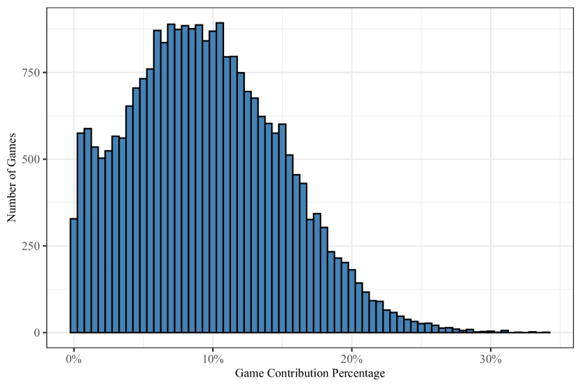
Figure 2: Game contribution percentage histogram. A distributional plot of the 25,892 non-zero GCP realizations for all players in the 2022-2023 NBA regular season. The GCP was computed using the methods of Section 2.1. For reference, the maximum realized GCP was by Luka Dončić at 33.8%, which occurred against the New York Knicks on December 27, 2023. This compares favorably to the 30-35% maximum player salary allowable under the NBA’s Collective Bargaining Agreement (National Basketball Association, 2018).

As a next set of results, we demonstrate how GCP may be used to assess the tipping point of a player who performs very well but has a tendency to miss games against a player that performs only reasonably well but does so consistently. The difficulty of comparing a high-performing player with many missed games against an average-performing player with few missed games has been a frequent source of consternation within the discourse of NBA pundits (for example, Lowe (2020) and Mannix and Beck (2023) frequently cite games missed as reasoning for preferring some players over others). Because a player receives a zero GCP for any missed game (see Figure 3), we may find the break even point by taking a running tally of GCP for the period in question, such as the entire 2022-2023 NBA regular season. In effect, we are taking a present value of all GCPs at an interest rate of 0%. That is, for active NBA player $p^{*}$ on team $t^{*}\in\mathcal{T}$ with $\bm{g}_{*}=\{g^{*}_{1},\ldots,g^{*}_{82}\}$ representing the ordered sequence of games in $\mathcal{G}$ of which $t^{*}$ appeared, we have

$$\text{PVGCP}_{p^{*}}=\sum_{\bm{g}_{*}}\text{GCP}^{g^{*}}_{t^{*},p^{*}}.$$ (9)

As with (7), the adjustments to (9) are natural for any players traded over the time period in question. We emphasize that (9) is directly comparable for all NBA players and does not require standardization, such as per 100 possessions. This allows for analysts to use a single metric to understand the impact of a player’s missed games, rather than computing a metric, standardizing it, and then attempting to perform additional missed game value judgments (e.g., Lowe, 2020; Mannix and Beck, 2023).

Table 4 presents the top fifty players in terms of PVGCP for the 2022-2023 NBA regular season. We can see the top five performers are Damontas Sabonis, Nikola Jokić, Joel Embiid, Luka Dončić, and Bam Adebayo. In general, our PVGCP metric arrives at a similar list of top performers, as measured by the 2022-2023 Kia NBA Most Valuable Player award voting (Associated Press, 2023a) and 2022-2023 Kia All-NBA selections (Associated Press, 2023b). The PVGCP metric prefers Sabonis as the top performer, whereas Embiid won the Kia NBA Most Valuable Player award. Table 4 has Embiid ranked 3rd in terms of PVGCP, though Embiid was the top per game GCP performer. Further, the PVGCP metric has Sabonis at a clear top spot, but he received only one 4th place MVP vote and 24 5th place votes. Hence, it is not unreasonable to suggest that our GCP methodology is able to capture Sabonis’ consistent high level of contribution to his team’s on court performance and availability in a way that other popular advanced metrics may overlook (that said, the win shares approach (Sports Reference LLC, 2022) had Sabonis ranked second behind Jokić (Sports Reference LLC, 2023a)). Aside from win shares, no other Table 4 metric had Sabonis higher than 7th. Further, all comparative metrics reported in Table 4 have Nikola Jokić as the top performer, which suggests that these popular advanced metrics may rely on similar overall approaches and not offer enough diversity of perspective. For completeness, we note Berri and Bradbury (2010) offers a critique of sports metrics proposed outside the scope of academic peer-review.

In this regard, we emphasize again that GCP is a measure of a player’s total contribution to his team’s on court performance; it does not attempt to parse out “good” and “bad” performance (review Section 2.1 as needed). This helps explain why players like Alperen Şengün and Nikola Vucečić have high values of PVGCP despite playing for teams in the Houston Rockets and Chicago Bulls that amassed paltry win percentages of 0.268 and 0.488, respectively (National Basketball Association, 2023c). As a further reflective note, it appears PVGCP is partial to the traditional big man in that there is a healthy representation of centers with high games played that were not recognized on many NBA award ballots (e.g., Vucečić, Şengün, Claxton, Gobert, Zubac, Porziņģis, Valančiūnas, Plumlee, Pöltl, Looney, and Okongwu). Then again, the importance of the center position has been long established in basketball treatments (e.g., Oliver, 2004, pg. 40), and more generally its depth of representation in Table 4 is a useful insight for NBA player personnel decision-makers tasked with allocating a capped player salary pool.

Rank	Player	GP	PVGCP	GCPpg	PER	WS	BPM	VORP	RAPTOR
1	Domantas Sabonis	79	16.81	0.213	23.50	12.60	5.80	5.40	8.66
2	Nikola Jokić	69	15.04	0.218	31.50	14.90	13.00	8.80	20.31
3	Joel Embiid	66	14.81	0.224	31.40	12.30	9.20	6.40	12.82
4	Luka Dončić	66	14.24	0.216	28.70	10.20	8.90	6.60	12.98
5	Bam Adebayo	75	14.10	0.188	20.10	7.40	1.50	2.30	5.69
6	Giannis Antetokounmpo	63	13.62	0.216	29.00	8.60	8.50	5.40	9.31
7	Evan Mobley	79	13.61	0.172	17.90	8.50	1.70	2.50	3.85
8	Nikola Vucečić	82	13.50	0.165	19.10	8.30	2.70	3.20	1.91
9	Julius Randle	77	13.01	0.169	20.30	8.10	3.70	3.90	5.64
10	Alperen Şengün	75	12.94	0.173	19.70	5.20	1.40	1.90	5.18
11	Jayson Tatum	74	12.88	0.174	23.70	10.50	5.50	5.10	8.99
12	Pascal Siakam	71	12.54	0.177	20.30	7.80	3.10	3.40	4.50
13	Shai Gilgeous-Alexander	68	12.36	0.182	27.20	11.40	7.30	5.60	9.86
14	Anthony Edwards	79	12.34	0.156	17.40	3.80	1.00	2.10	6.42
15	Nic Claxton	76	12.25	0.161	20.80	9.20	3.10	2.90	5.57
16	Rudy Gobert	70	12.22	0.175	18.90	7.80	0.70	1.40	5.25
17	Ivica Zubac	76	12.15	0.160	16.70	6.70	-0.90	0.60	2.15
18	Trae Young	73	12.00	0.164	22.00	6.70	3.30	3.40	9.12
19	Anthony Davis	56	11.86	0.212	27.80	9.00	6.30	4.00	9.77
20	Brook Lopez	78	11.83	0.152	18.40	8.00	2.10	2.50	8.70
21	Paolo Banchero	72	11.57	0.161	14.90	2.40	-1.50	0.30	-0.42
22	Kristaps Porziņģis	65	11.44	0.176	23.10	7.70	4.30	3.40	8.24
23	Scottie Barnes	77	11.35	0.147	15.50	5.00	0.40	1.60	4.62
24	Jonas Valančiūnas	79	11.34	0.144	19.30	5.80	-0.40	0.80	0.55
25	Mason Plumlee	79	11.29	0.143	19.60	7.90	2.20	2.20	3.20
26	De’Aaron Fox	73	11.18	0.153	21.80	7.40	2.50	2.70	7.19
27	Jalen Brunson	68	11.16	0.164	21.20	8.70	3.90	3.50	8.14
28	Jakob Pöltl	72	11.16	0.155	21.00	6.00	1.90	1.90	3.45
29	DeMar DeRozan	74	11.14	0.151	20.60	8.50	2.00	2.60	7.38
30	Zach LaVine	77	11.04	0.143	19.00	7.10	1.90	2.70	5.53
31	Jarrett Allen	68	11.00	0.162	19.90	9.50	2.40	2.40	4.53
32	Fred VanVleet	69	10.94	0.159	17.00	6.50	2.50	2.90	10.01
33	Donovan Mitchell	68	10.76	0.158	22.90	8.90	6.30	5.00	9.45
34	Mikal Bridges	82	10.73	0.131	16.80	7.50	1.70	2.80	6.76
35	Jaylen Brown	67	10.68	0.159	19.10	5.00	1.30	2.00	4.12
36	Kevon Looney	82	10.61	0.129	17.80	8.70	2.10	2.00	6.09
37	Draymond Green	73	10.59	0.145	12.20	4.70	0.80	1.60	6.09
38	Spencer Dinwiddie	79	10.56	0.134	16.00	6.30	0.70	1.80	4.56
39	CJ McCollum	75	10.54	0.140	15.60	4.30	0.80	1.90	3.59
40	Dejounte Murray	74	10.49	0.142	17.00	4.70	1.00	2.10	3.07
41	Jordan Poole	82	10.46	0.128	14.60	3.20	-1.90	0.10	-0.44
42	Franz Wagner	80	10.44	0.130	15.90	5.40	-0.10	1.30	7.24
43	Jimmy Butler	64	10.40	0.162	27.60	12.30	8.70	5.80	10.11
44	Onyeka Okongwu	80	10.39	0.130	19.40	7.10	0.80	1.30	3.50
45	Damian Lillard	58	10.34	0.178	26.70	9.00	7.10	4.90	11.52
46	Jalen Green	76	10.30	0.136	14.50	1.80	-2.10	0.00	1.75
47	Ja Morant	61	10.30	0.169	23.30	6.00	5.70	3.80	8.39
48	Russell Westbrook	73	10.30	0.141	16.10	1.90	0.20	1.20	1.37
49	Darius Garland	69	10.29	0.149	18.80	7.60	2.40	2.70	8.95
50	James Harden	58	10.26	0.177	21.60	8.40	5.40	4.00	9.22

Table 4: Top performers: Absolute game contribution percentage. The top 50 performers in terms of (9) for the 2022-2023 NBA regular season. For reference, we also present the number of games played (GP), GCP per game (GCPpg), standard player efficiency rating (PER) (Sports Reference LLC, 2023a), win shares (WS) (Sports Reference LLC, 2023a), box plus/minus (BPM) per 100 possessions (Sports Reference LLC, 2023a), value over replacement player (VORP) (Sports Reference LLC, 2023a), and regular season wins above replacement (RAPTOR) (FiveThirtyEight, 2023) for each player. The high value in each column has been noted in bold.

It is interesting to observe that there are multiple ways to obtain an impressive PVGCP. As we’ve established, it is clear that players with any missed games will be directly penalized in (9) in a way that differs from metrics based on cumulative on court statistics. Nonetheless, it is possible for a player to perform so well in games played that they can amass a high PVGCP despite accumulating many missed games. With PVGCP, we can obtain this exact inflection point. This is the value of treating missed games as defaults, and it may offer useful insights on its own merit. Consider Figure 3, which compares Anthony Davis and Brook Lopez. From Table 4, we can see that Davis and Lopez accumulated nearly identical PVGCPs at 11.86 and 11.83, respectively. Davis did so in 56 games (i.e., 26 defaults) whereas Lopez did so in 78 games (i.e., only 4 defaults). The visual representation in Figure 3 makes the difference in consistency readily apparent. In other words, Lopez, through his consistent availability and steady performance in 78 games was able to reach the same level of PVGCP as Davis for the 2022-2023 NBA season. Because Lopez earned $13,906,976 in comparison to Davis at $37,980,720 for the 2022-2023 NBA season (HoopsHype, 2023), this information may be of interest to NBA player personnel decision makers. (Davis had a very strong 2023 NBA postseason, which is an important consideration not made within this analysis.) We arrive at the formal ROI calculations in Section 3.3.

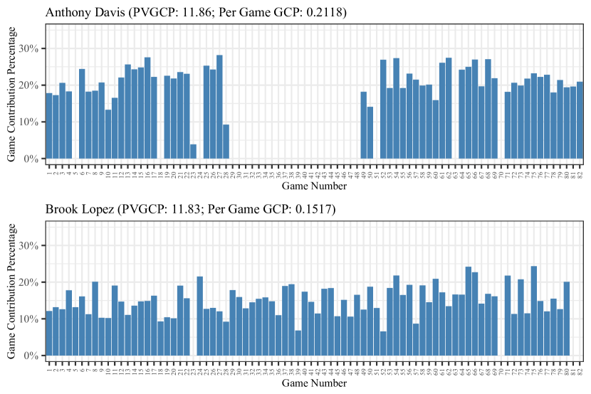
Figure 3: Game contribution percentage comparison. A game-by-game plot of GCP for Anthony Davis (top) and Brook Lopez (bottom) for the 2022-2023 NBA regular season. Both Davis and Lopez registered nearly an identical PVGCP (i.e., (9)) at 11.86 and 11.83, respectively, despite a large difference in games played (56 versus 78, respectively). Because GCP is a single game calculation, it treats missed games as defaults. Hence, Davis missed enough games and Lopez played enough games to register a similar level of cumulative contribution as measured by PVGCP. Because Lopez earned $13,906,976 in comparison to Davis at $37,980,720 for the 2022-2023 NBA regular season (HoopsHype, 2023), this information may be of interest to NBA player personnel decision makers.

3.3 Return on Investment

The final component of our effort and the ultimate purpose of this study is to combine the absolute GCP results of Table 4 with each player’s salary to perform a contractual realized ROI calculation in the form of (8). The first step is to calculate the SGV proposed in (5). Based on our data of 547 active NBA players for the 2022-2023 NBA season, we have $\mathcal{S}=$ $4,472,678,188. Thus, $\text{SGV}=$ $1,818,162. To avoid skewed calculations from players on 10-day contracts, we set a minimum games played requirement of 25 games. This limits the calculation pool to 423 players. The top and bottom 50 performers in terms of ROI, $r$, via (8), have been compiled in Tables 5 and 6, respectively. There are some interesting observations.

We begin with the top performers. Immediately, we see that the highest salary in Table 5 is $4.215M, which belongs to Tyrese Haliburton. Because this salary is well below the mean (median) player salary of $10.022M ($5.122M) for all players playing at least 25 games during the 2022-2023 NBA regular season, it is clear that the biggest returns belong to players signed to small value contracts that also contribute meaningfully in terms of on court production. In other words, the ROI calculation prefers players with a small initial investment (i.e., $\text{CF}_{0}$ in Figure 1) that produce valuable game-by-game output (i.e., $\text{CF}_{i}$, $1\leq i\leq 82$ in Figure 1). This insight is perhaps elementary, but the methods we propose lead to a direct framework to identify which players have outperformed their salaries and by how much, neither of which is a straightforward calculation. If we combine this information with the NBA team salary cap restrictions, then it may be used to identify market inefficiencies in hopes of optimizing team roster construction. On the player side, this information may be used in upcoming contract negotiations. (It is notable that a number of players in Table 5 have signed contracts with large raises for the upcoming 2023-2024 NBA season: e.g., Tre Jones, Max Strus, Austin Reaves, Jock Landale, Desmond Bane, Gabe Vincent, Jordan Poole, Shake Milton, Tyrese Haliburton (Associated Press, 2023c)). Additionally, it is of interest to observe that there is limited overlap with Table 4. Indeed, only Alperen Şengün and Jordan Poole appear in both tables. This again highlights the importance of the initial investment in calculating an ROI with (8).

Rank	Player	Salary	GP	PVGCP	ROI (%)
1	Tre Jones	$1.783	68	8.228	0.132
2	Kevon Harris	$0.509	34	1.778	0.122
3	Nick Richards	$1.783	65	6.766	0.113
4	Ayo Dosunmu	$1.564	80	6.921	0.108
5	Max Strus	$1.816	80	7.336	0.106
6	Anthony Lamb	$0.695	62	4.734	0.096
7	Christian Koloko	$1.500	58	3.851	0.095
8	Austin Reaves	$1.564	64	6.594	0.094
9	Jock Landale	$1.564	69	5.546	0.094
10	Jose Alvarado	$1.564	61	5.475	0.092
11	Jaden McDaniels	$2.161	79	8.587	0.087
12	Daniel Gafford	$1.931	78	9.111	0.086
13	Kevin Porter Jr.	$3.218	59	8.968	0.086
14	Kenyon Martin Jr.	$1.783	82	7.208	0.086
15	Santi Aldama	$2.094	77	6.385	0.080
16	Desmond Bane	$2.130	58	7.823	0.079
17	Bol Bol	$2.200	70	5.524	0.077
18	Alperen Şengün	$3.375	75	12.943	0.077
19	Drew Eubanks	$1.968	78	8.166	0.077
20	Herbert Jones	$1.785	66	7.614	0.076
21	Jordan Goodwin	$1.280	62	5.189	0.075
22	Naji Marshall	$1.783	77	6.417	0.073
23	Immanuel Quickley	$2.316	81	8.902	0.073
24	Gabe Vincent	$1.816	68	6.048	0.073
25	Tyrese Maxey	$2.727	60	7.274	0.073
26	Dennis Smith Jr.	$2.133	54	5.776	0.068
27	Jaylen Nowell	$1.931	65	4.538	0.067
28	Terance Mann	$1.931	81	6.528	0.066
29	Kenrich Williams	$2.000	53	5.004	0.065
30	Orlando Robinson	$0.386	31	2.111	0.063
31	Aaron Wiggins	$1.564	70	4.695	0.062
32	Naz Reid	$1.931	68	6.862	0.060
33	Troy Brown Jr.	$1.968	76	5.707	0.060
34	Isaiah Stewart	$3.433	50	6.489	0.059
35	Jeremiah Robinson-Earl	$2.000	43	3.277	0.059
36	Walker Kessler	$2.696	74	9.751	0.059
37	Duane Washington Jr.	$0.629	31	1.735	0.058
38	Wenyen Gabriel	$1.879	68	5.852	0.057
39	John Konchar	$2.300	72	5.006	0.057
40	Jordan Poole	$3.901	82	10.461	0.056
41	Shake Milton	$1.998	76	5.524	0.056
42	Andrew Nembhard	$2.244	75	6.998	0.056
43	Damion Lee	$2.133	74	4.725	0.054
44	Isaiah Jackson	$2.574	63	5.796	0.054
45	Isaiah Livers	$1.564	52	3.818	0.054
46	Keldon Johnson	$3.873	63	8.391	0.053
47	Tyrese Haliburton	$4.215	56	7.964	0.053
48	Javonte Green	$1.816	32	2.074	0.052
49	Trendon Watford	$1.564	62	5.130	0.051
50	Jericho Sims	$1.640	52	3.731	0.049

Table 5: Top 50 performers: Return on investment. The top 50 performers in terms of (8) for the 2022-2023 NBA regular season, based on a minimum of 25 games played. For reference, we also include the player salary (HoopsHype, 2023) in millions, games played (GP), and PVGCP, as calculated with (9).

The lowest returns in Table 6 offer another set of interesting observations. As expected, there are many large contracts in Table 6, many of which are well above the 75th percentile salary of $13.64M for all players playing at least 25 games during the 2022-2023 NBA regular season. As the opposite reasoning of the previous paragraph would suggest, it requires much stronger on court performance (i.e., $\text{CF}_{i}$, $1\leq i\leq 82$) to overcome a much higher initial investment (i.e., $\text{CF}_{0}$). In addition, there are many highly decorated NBA players in Table 6, such as Stephen Curry, LeBron James, Kevin Durant, and Giannis Antetokounmpo. This may be surprising at first glance, but we offer a few reasonable explanations. First, many players in Table 6 missed games in the 2022-2023 NBA regular season. Quite simply, it is difficult to overcome a large initial investment with many subsequent zero cash flows. Second, we do not include playoff games in the calculations for Table 6. If NBA personnel decision makers put a premium on playoff performance (a very reasonable supposition), then the calculations in Table 6 are missing an important component of the contractual value of the highest paid NBA players. Similarly, we only consider on court performance, and we ignore off court value vis-á-vis jersey sales, ticket sales, television revenue, and other potential pecuniary production that is a likely income component to teams rostering the NBA’s most popular players. We attempted to value on court performance only by design, but this is a straightforward adjustment to the ROI framework we propose. Additional related discussion may be found in Section 4. As a final reference point, the highest 2022-2023 salary was $48.07, which belonged to Stephen Curry. Assuming all 82 games played, the break-even IRR implies a per game cash flow of $0.586M. Assuming an SGV of $1.818M, as calculated above, this implies a per game GCP of 32.24%. Again, this is quite close to the maximum player salary of 30-35% per the NBA’s CBA (National Basketball Association, 2018) and is an additional informal validation of our approach.

Rank	Player	Salary	GP	PVGCP	ROI (%)
423	Derrick Rose	$14.521	27	1.23	-0.080
422	John Wall	$47.346	34	3.51	-0.070
421	Evan Fournier	$18.000	27	1.33	-0.047
420	Andrew Wiggins	$33.617	37	4.76	-0.039
419	Ben Simmons	$35.449	42	5.33	-0.038
418	Garrett Temple	$5.156	25	0.52	-0.037
417	Duncan Robinson	$16.902	42	2.10	-0.032
416	Richaun Holmes	$11.215	42	1.53	-0.032
415	Karl-Anthony Towns	$33.833	29	4.58	-0.031
414	Davis Bertans	$16.000	45	1.62	-0.030
413	Khris Middleton	$37.984	33	3.63	-0.029
412	Bradley Beal	$43.279	50	7.11	-0.026
411	Stephen Curry	$48.070	56	8.72	-0.023
410	LeBron James	$44.475	55	9.15	-0.022
409	Kyle Lowry	$28.333	55	6.81	-0.022
408	Zion Williamson	$13.535	29	4.67	-0.022
407	Klay Thompson	$40.600	69	7.26	-0.022
406	Gordon Hayward	$30.075	50	5.49	-0.022
405	Paul George	$42.492	56	9.24	-0.021
404	Tobias Harris	$37.633	74	8.33	-0.020
403	Bryn Forbes	$2.298	25	0.71	-0.020
402	Michael Porter Jr.	$30.914	62	6.29	-0.020
401	Collin Sexton	$16.700	48	4.66	-0.020
400	Wendell Moore Jr.	$2.307	29	0.53	-0.020
399	Furkan Korkmaz	$5.000	37	1.13	-0.020
398	Kawhi Leonard	$42.492	52	7.98	-0.019
397	Joe Harris	$18.643	74	4.85	-0.019
396	Boban Marjanovic	$4.101	31	0.80	-0.019
395	Damian Lillard	$42.492	58	10.34	-0.018
394	Patty Mills	$6.479	40	1.68	-0.018
393	Matthew Dellavedova	$2.629	32	0.68	-0.018
392	Brandon Ingram	$31.651	45	6.60	-0.017
391	DeAndre Jordan	$10.734	39	3.11	-0.017
390	Devin Booker	$33.833	53	8.52	-0.017
389	Myles Turner	$35.097	62	9.60	-0.017
388	Al Horford	$26.500	63	6.92	-0.016
387	Kevin Durant	$44.120	47	7.86	-0.016
386	Steven Adams	$17.927	42	6.66	-0.016
385	Kira Lewis Jr.	$4.004	25	0.91	-0.015
384	Gary Harris	$13.000	48	3.17	-0.015
383	Robert Covington	$12.308	48	3.33	-0.015
382	Doug McDermott	$13.750	64	4.07	-0.015
381	Landry Shamet	$9.500	40	2.83	-0.015
380	Chris Paul	$28.400	59	7.52	-0.015
379	Jimmy Butler	$37.653	64	10.40	-0.014
378	Jrue Holiday	$34.320	67	9.82	-0.014
377	Nicolas Batum	$19.700	78	5.70	-0.014
376	Jamal Murray	$31.651	65	9.22	-0.014
375	Zach LaVine	$37.097	77	11.04	-0.013
374	Giannis Antetokounmpo	$42.492	63	13.62	-0.013

Table 6: Bottom 50 performers: Return on investment. The bottom 50 performers in terms of (8) for the 2022-2023 NBA regular season, based on a minimum of 25 games played. For reference, we also include the player salary (HoopsHype, 2023) in millions, games played (GP), and PVGCP, as calculated with (9).

As a final curiosity of the ROI framework we propose, it is of interest to examine a scatter plot of ROI by salary. In other words, player compensation in the NBA is effectively formulaic and prescribed by the National Basketball Association (2018). Thus, for players bracketed within certain salary ranges, it is useful to identify which players generate the relative best contractual ROI. We do exactly this in Figure 4. The best relative performers are at the top of the resulting hockey stick shape, e.g., by increasing player salary: Tre Jones, Kevin Porter Jr., Franz Wagner, Evan Mobley, Brook Lopez, Domantas Sabonis, Nikola Jokić, Giannis Antetokoumpo, and Russell Westbrook. Conversely, the worse relative performers are at the bottom of the hockey stick shape, e.g., Bryn Forbes, Patty Mills, Landry Shamet, Richaun Holmes, Duncan Robinson, Kyle Lowry, Andrew Wiggins, and Bradley Beal. Furthermore, the overall shape of the scatter plot in Figure 4 is itself instructive. Because it is difficult for higher salary players to generate a break-even ROI based only on regular season on court performance, Figure 4 implies that a considerable component of the expectation for maximum salary players is play-off performance. As a final caveat, the results will likely change with a different single game metric, different game values, or methods that go beyond just on court performance. Further discussion may be found in Section 4.

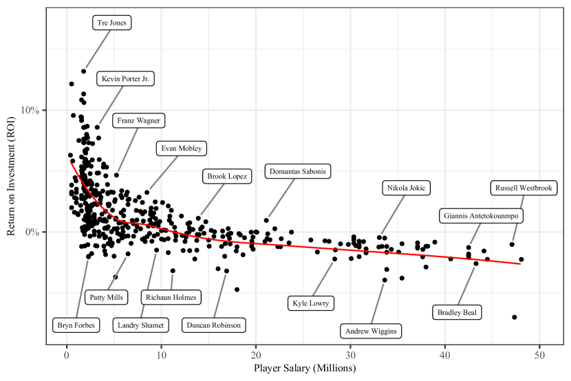
Figure 4: Relative return on investment by salary. A scatter plot of contractual ROI by salary via (8) for the 2022-2023 NBA regular season. Because player salary is generally deterministic by National Basketball Association (2018), this plot allows for relative comparisons within each salary bracket. For example, for players in the $30M-$35M range, Nikola Jokić generated a higher relative regular season ROI than Andrew Wiggins. The mean line was generated by the loess function in R Core Team (2022). The scatter plot shape is of interest, too, as it demonstrates maximum salary players generally struggle to produce a break-even ROI based on regular season performance only.

4 Discussion

The NBA is big business, and no small part is due to the over $4.4 billion in annual player compensation (HoopsHype, 2023). Given the salary cap restrictions of the NBA (National Basketball Association, 2018), it is of paramount importance to team on court success to appropriately compensate players for on court performance. Despite this, there are no known studies that present a framework to measure a player’s contractual ROI. This study is thus the first known attempt.

Our approach unfolds in five parts. We first decide on an investment time horizon over which performance will be measured. The next step is computing a GCP metric. (The GCP we propose in Section 2.1, via (1), is itself a novel contribution to the field of on court basketball player assessment metrics. Because (1) is calculated per game, cumulative metrics such as PVGCP, via (9), allow analysts to assess the impact of missed games in a single calculation (e.g., Figure 3). This has long been a known issue in the NBA (Wimbish, 2023). Additionally, PVGCP may offer a fresh perspective on player evaluation, given the general consensus of the other popular player evaluation metrics reported in Table 4; i.e., PER, WS, BPM, VORP, and RAPTOR unanimously ranking Jokić first, whereas PVGCP ranks Sabonis first.) After calculating GCP, the third step is to estimate the dollar value of each NBA game in the measurement period (e.g., the SGV). Fourth, the GCP and SGV calculations are combined to convert a player’s on court per game performance into a series of realized cash flows. From this, the fifth and final step is to perform standard financial calculations by using the player’s salary as invested (i.e., negative) cash flows and the newly created income (i.e., positive) cash flows from step four. Our novel framework is summarized in Figure 5.

Figure 5: NBA contractual ROI estimation framework summary.

The potential value of our proposed framework is illustrated in Figure 4, which may be used by NBA player personnel decision makers and NBA player agents alike in contract negotiations. Additionally, voters for NBA regular season awards may be interested in the results of Table 4 or 5. Indeed, the Kia NBA Most Valuable Player award seems like a good candidate for the consideration of PVGCP or ROI-type calculations. In terms of forecasting, it is not difficult to see how player on court projections may be used to produce a distribution of GCP realizations, which may then be used to estimate the dollar or trade value of draft picks or swaps or for potential trades more generally. Further, because player contracts are highly regulated by the NBA CBA (National Basketball Association, 2018), the ROI calculation methods herein may also be used for validation and fairness purposes (e.g., Figure 2 and the break-even calculations of Section 3.3 suggest the maximum salary restriction of 30-35% of a team’s salary cap appears reasonable). GCP may also be used in sports injury-related or performance-based studies. For example, Page et al. (2013) look at the effect of minutes played and usage on a player’s production curve over the course of their career. Within the model, the Game Score (Sports Reference LLC, 2023b) is used as a measure of production. Our GCP offers an alternative measure for a similar analysis.

In closing, we again emphasize the main contribution of this study is a framework to measure realized contractual ROI for NBA players. As such, some simplifying assumptions have been made, and it is possible our methodology may be customized or enhanced. For example, the fields we select for the GCP calculation in Table 1 are just one such proposal. These may be easily edited to meet the likely differing views of NBA analysts (NBA teams may also possess more detailed player evaluation data than what is publicly available, which is a further motivation for alternative field selections). Further, in (1), we use a simple, uniform-like weighting system for the importance of each field in Table 1. Alternative weighting schemes are also possible. For example, Özmen (2016) analyzes the marginal contribution of game statistics across various levels of competitiveness in the Euroleague to win probability. Hence, a similar analysis could be utilized to vary the weighting scheme of (1), if desired. Instead, additional precision may be used to assign the weights within GCP, such as refining the quality of a field-goal attempt (e.g., Shortridge et al., 2014; Daly-Grafstein and Bornn, 2019) or accounting for peer (i.e., teammate) and non-peer (i.e., opponent) effects (e.g., Horrace et al., 2022). Even more, the GCP may be ignored altogether and replaced with an alternative per game evaluation metric. As long as the percentage and per game properties hold, many alternatives to GCP are valid.

Beyond changes to the GCP metric, the ROI methods of Section 2.2 may be enhanced or customized, too. For example, we assume the entire player salary is a time zero investment. Instead, the actual payment dates of a player’s salary may be used. In the same way, the actual game dates may be used instead of assuming 82 equally spaced per game cash flows. Further, we use a uniform weight for each game, and the nature of (8) implicitly weights early season games more heavily than later season games. As an alternative, it may be desirable to assign different weights to each game based on its importance (i.e., the proverbial “big game”). For example, Teramoto and Cross (2010) is an an example of how weighting schemes may differ for playoff games versus regular season games in the NBA. Or, to avoid the implicit weighting of (8), it may be prudent to randomize the order of the games and calculate a distribution of realized ROI calculations. Indeed, the SGV methodology of (5) is quite rudimentary and is thus ripe for additional study. Furthermore, we consider only regular season games. While this is natural for regular season award considerations, there is the obvious curiosity of how the calculations in Section 3.3 would change with the inclusion of playoff games or even off court revenue, such as jersey sales. We close with a hopeful note in that the suggestions of this and the previous paragraph may motivate additional study.

References

- Associated Press (2022) Associated Press (2022). “Doncic has 60-21-10, rallies Mavs to wild OT win over Knicks.” https://www.ESPN.com - Entertainment and Sports Programming Network. https://www.espn.com/nba/recap/_/gameId/401468667. Online; accessed 24 July 2023.
- Associated Press (2023a) Associated Press (2023a). “76ers center Joel Embiid wins 2022-23 Kia NBA Most Valuable Player award.” nba.com. https://www.nba.com/news/2022-23-kia-nba-most-valuable-player-award. Online; accessed 24 July 2023.
- Associated Press (2023b) Associated Press (2023b). “Joel Embiid, Giannis Antetokounmpo, Luka Doncic lead 2022-23 Kia All-NBA 1st Team.” nba.com. https://www.nba.com/news/2022-23-all-nba-teams-announced. Online; accessed 24 July 2023.
- Associated Press (2023c) Associated Press (2023c). “NBA free agency 2023: Latest signings, news, buzz and reports.” https://www.ESPN.com - Entertainment and Sports Programming Network. https://www.espn.com/nba/story/_/id/37852244/nba-free-agency-2023-latest-deals-news-buzz-reports. Online; accessed 25 July 2023.
- Berk and Demarzo (2007) J. Berk and P. Demarzo (2007). Corporate Finance, 1st Edition. Pearson Education, Inc.
- Berri (1999) D. J. Berri (1999). “Who is ‘most valuable’? Measuring the player’s production of wins in the National Basketball Association.” Managerial and Decision Economics 20, 411–427.
- Berri and Bradbury (2010) D. J. Berri and J. C. Bradbury (2010). “Working in the land of the metricians.” Journal of Sports Economics 11, 29–47.
- Berri et al. (2005) D. J. Berri, S. L. Brook, B. Frick, A. J. Fenn and R. Vicente-Mayoral (2005). “The short supply of tall people: Competitive imbalance and the National Basketball Association.” Journal of Economic Issues 39, 1029–1041.
- Berri et al. (2007) D. J. Berri, S. L. Brook and M. B. Schmidt (2007). “Does one simply need to score to score?” International Journal of Sport Finance 2, 190–205.
- Berri and Krautmann (2006) D. J. Berri and A. C. Krautmann (2006). “Shirking on the court: Testing for the incentive effects of guaranteed pay.” Economic Inquiry 44, 536–546.
- Casals and Martínez (2013) M. Casals and J. A. Martínez (2013). “Modelling player performance in basketball through mixed models.” International Journal of Performance Analysis in Sport 13, 64–82.
- Daly-Grafstein and Bornn (2019) D. Daly-Grafstein and L. Bornn (2019). “Rao-blackwellizing field goal percentage.” Journal of Quantitative Analysis in Sports 15, 85–95.
- Fearnhead and Taylor (2011) P. Fearnhead and B. M. Taylor (2011). “On estimating the ability of NBA players.” Journal of Quantitative Analysis in Sports 7.
- FiveThirtyEight (2023) FiveThirtyEight (2023). “The best NBA players, according to RAPTOR.” FiveThirtyEight.com. https://projects.fivethirtyeight.com/nba-player-ratings/. Online; accessed 25 July 2023.
- Halevy et al. (2012) N. Halevy, E. Y. Chou, A. D. Galinsky and J. K. Murnighan (2012). “When hierarchy wins: Evidence from the National Basketball Association.” Social Psychological and Personality Science 3, 398–406.
- HoopsHype (2023) HoopsHype (2023). “2022/23 NBA Player Salaries.” hoopshype.com. https://hoopshype.com/salaries/players/2022-2023/. Online; accessed 12 June 2023.
- Horrace et al. (2022) W. C. Horrace, H. Jung and S. Sanders (2022). “Network competition and team chemistry in the NBA.” Journal of Business & Economic Statistics 40, 35–49.
- Hughes and Cain (2011) J. Hughes and L. P. Cain (2011). American Economic History, Eighth Edition. Addison Wesley.
- Idson and Kahane (2000) T. Idson and L. Kahane (2000). “Team effects on compensation: An application to salary determination in the National Hockey League.” Economic Inquiry 38, 345–357.
- Kuehn (2017) J. Kuehn (2017). “Accounting for complementary skill sets: Evaluating individual marginal value to a team in the National Basketball Association.” Economic Inquiry 55, 1556–1578.
- Lackritz and Horowitz (2021) J. Lackritz and I. Horowitz (2021). “The value of statistics contributing to scoring in the NBA: A quantitative approach.” The American Economist 66, 175–189.
- Lowe (2020) Z. Lowe (2020). “2020 NBA awards ballot: Zach Lowe’s picks for All-NBA, All-Defensive and All-Rookie.” https://www.ESPN.com - Entertainment and Sports Programming Network. https://www.espn.com/nba/story/_/id/29541185/2020-nba-awards-ballot-zach-lowe-picks-all-nba-all-defensive-all-rookie. Online; accessed 24 July 2023.
- Mahoney (2019) R. Mahoney (2019). “The 16-game player: Why Draymond Green thrives in the NBA playoffs.” Sports Illustrated. https://www.si.com/nba/2019/05/29/draymond-green-warriors-raptors-2019-nba-finals-stephen-curry-kevin-durant. Online; accessed 20 July 2023.
- Mankiw (2003) N. G. Mankiw (2003). Principles of Macroeconomics, 3rd Edition. South-Western College Pub.
- Mannix and Beck (2023) C. Mannix and H. Beck (2023). “Breaking down the biggest NBA All-Star surprises and snubs.” https://www.SI.com - Sports Illustrated. https://www.si.com/nba/2023/02/03/nba-all-star-surprises-snubs-2023. Online; accessed 24 July 2023.
- Martínez (2012) J. A. Martínez (2012). “Factors determining production (FDP) in basketball.” Economics and Business Letters 1, 21–29.
- National Basketball Association (2018) National Basketball Association (2018). “Highlights of the Collective Bargaining Agreement between the National Basketball Association (NBA) and National Basketball Players Association (NBPA).” nba.com. https://cdn.nba.com/manage/2021/03/2018-19-CBA.pdf. Online; accessed 19 July 2023.
- National Basketball Association (2022) National Basketball Association (2022). “NBA salary cap for 2022-23 season set at just over $123 million.” nba.com. https://www.nba.com/news/nba-salary-cap-for-2022-23-season-set-at-just-over-123-million. Online; accessed 30 June 2023.
- National Basketball Association (2023a) National Basketball Association (2023a). “Glossary.” nba.com. https://www.nba.com/stats/help/glossary. Online; accessed 13 June 2023.
- National Basketball Association (2023b) National Basketball Association (2023b). “Schedule.” nba.com. https://www.nba.com/schedule. Online; accessed 23 June 2023.
- National Basketball Association (2023c) National Basketball Association (2023c). “Standings.” nba.com. https://www.nba.com/standings. Online; accessed 8 September 2023.
- National Basketball Association (2023d) National Basketball Association (2023d). “Statistics.” nba.com. https://www.nba.com/stats. Online; accessed 13 June 2023.
- Niemi (2010) J. B. Niemi (2010). “Evaluating individual player contributions to team offense and defense: A model based approach.” JSM Proceedings, Section on Statistics in Sports, Vancouver, BC, Canada: American Statistical Association.
- Oliver (2004) D. Oliver (2004). Basketball on Paper: Rules and Tools for Performance Analysis. Potomac Books, Inc.
- Özmen (2016) M. U. Özmen (2016). “Marginal contribution of game statistics to probability of winning at different levels of competition in basketball: Evidence from the Euroleague.” International Journal of Sports Science & Coaching 11, 98–107.
- Page et al. (2013) G. L. Page, B. J. Barney and A. T. McGuire (2013). “Effect of position, usage rate, and per game minutes played on NBA player production curves.” Journal of Quantitative Analysis in Sports 9, 337–345.
- Page et al. (2007) G. L. Page, G. W. Fellingham and C. S. Reese (2007). “Using box-scores to determine a position’s contribution to winning basketball games.” Journal of Quantitative Analysis in Sports 3.
- Patel (2018) S. Patel (2018). “nba_api: An API client package to access the APIs of NBA.com.” GitHub repository. https://github.com/swar/nba_api. Online; accessed 21 July 2023 (v1.2.0).
- R Core Team (2022) R Core Team (2022). R: A language and environment for statistical computing. R Foundation for Statistical Computing, Vienna, Austria.
- Rappaport (2023) M. Rappaport (2023). “The definitive history of ‘Trust the Process’.” https://bleacherreport.com/ - Bleacher Report, Inc. https://bleacherreport.com/articles/2729018-the-definitive-history-of-trust-the-process. Online; accessed 8 September 2023.
- Shortridge et al. (2014) A. Shortridge, K. Goldsberry and M. Adams (2014). “Creating space to shoot: Quantifying spatial relative field goal efficiency in basketball.” Journal of Quantitative Analysis in Sports 10, 303–313.
- Simmons and Berri (2011) R. Simmons and D. J. Berri (2011). “Mixing the princes and the paupers: Pay and performance in the National Basketball Association.” Labour Economics 18, 381–388. The Economics of Sports Labour Markets.
- Sports Reference LLC (2022) Sports Reference LLC (2022). “NBA Win Shares.” Basketball-Reference.com - Basketball Statistics and History. https://www.basketball-reference.com/about/ws.html. Online; accessed 27 December 2022.
- Sports Reference LLC (2023a) Sports Reference LLC (2023a). “2022-23 NBA Leaders.” Basketball-Reference.com - Basketball Statistics and History. https://www.basketball-reference.com/leagues/NBA_2023_leaders.html. Online; accessed 24 July 2023.
- Sports Reference LLC (2023b) Sports Reference LLC (2023b). “Glossary.” Basketball-Reference.com - Basketball Statistics and History. https://www.basketball-reference.com/about/glossary.html. Online; accessed 26 January 2023.
- Spotrac (2023) Spotrac (2023). “Contract Details.” Spotrac.com. https://www.spotrac.com/nba/portland-trail-blazers/chance-comanche-82139/. Online; accessed 25 July 2023.
- Teramoto and Cross (2010) M. Teramoto and C. L. Cross (2010). “Relative importance of performance factors in winning NBA games in regular season versus playoffs.” Journal of Quantitative Analysis in Sports 6.
- Terner and Franks (2021) Z. Terner and A. Franks (2021). “Modeling player and team performance in basketball.” Annual Review of Statistics and Its Application 8, 1–23.
- Tunaru et al. (2005) R. Tunaru, E. Clark and H. Viney (2005). “An option pricing framework for valuation of football players.” Review of Financial Economics 14, 281–295. Real Options SI.
- Varma (2021) J. Varma (2021). jrvFinance: Basic finance; NPV/IRR/annuities/bond-Pricing; Black Scholes. R package version 1.4.3.
- Wight (2015) J. B. Wight (2015). Ethics in Economics: An Introduction to Moral Frameworks. Stanford University Press.
- Wimbish (2023) J. Wimbish (2023). “NBA CBA: New details emerge about in-season tournament, 65-game threshold for MVP, other awards.” https://www.cbssports.com/ - CBS Sports. https://www.cbssports.com/nba/news/nba-cba-new-details-emerge-about-in-season{}-tournament-65-game-threshold-for-mvp-other-awards/. Online; accessed 28 July 2023.
- Wojnarowski (2022) A. Wojnarowski (2022). “Mat Ishbia agrees to Suns purchase for record $4 billion.” https://www.ESPN.com - Entertainment and Sports Programming Network. https://www.espn.com/nba/story/_/id/35292815/sources-mat-ishbia-finalizing-suns-purchase-4-billion. Online; accessed 30 June 2023.