The Effect of Intrinsic Dimension on Learning a Mahalanobis Metric under Compression

Abstract

Metric learning aims at finding a suitable distance metric over the input space, to improve the performance of distance-based learning algorithms. In high-dimensional settings, it can also serve as dimensionality reduction by imposing a low-rank restriction to the learnt metric. In this paper, we consider the problem of learning a Mahalanobis metric, and instead of training a low-rank metric on high-dimensional data, we use a randomly compressed version of the data to train a full-rank metric in this reduced feature space. We give theoretical guarantees on the error for Mahalanobis metric learning, which depend on the stable dimension of the data support, but not on the ambient dimension. Our bounds make no assumptions aside from i.i.d. data sampling from a bounded support, and automatically tighten when benign geometrical structures are present. An important ingredient is an extension of Gordon’s theorem, which may be of independent interest. We also corroborate our findings by numerical experiments.

1 INTRODUCTION

In clustering and classification, there have been numerous distance-based algorithms proposed. While the Euclidean metric is the “standard” notion of distance between numerical vectors, it does not always result in accurate learning. This can be e.g. due to the presence of many dependent features, noise, or features with large ranges that dominate the distances [1]. Mahalanobis metric learning aims at lessening this caveat by linearly transforming the feature space in a way that properly weights all important features, and discards redundant ones. In its most common form, metric learning focuses on learning a Mahalanobis metric [2, 3, 4].

Metric learning algorithms can be divided into two types based on their purpose [1]. Distance-based metric learning aims to increase the distances between instances of different classes (inter-class distances) and decrease the distances inside the same class (intra-class distances). On the other hand, classifier-based metric learning focuses on directly improving the performance of a particular classification algorithm, and is therefore dependent on the algorithm in question. Examples of both types of algorithms abound in the literature, see e.g. [5] and references therein.

Despite the success of Mahalanobis metric learning, high-dimensionality of the data is a provable bottleneck that arises fairly often in practice. The work of [1] has shown through both upper and lower bounds that the sample complexity of Mahalanobis metric learning in general case increases linearly with the data dimension. In addition, so does the computational complexity. Indeed, high-dimensionality is known to quickly degrade the performance of machine learning algorithms in practice. This means that, even if a suitable distance metric is found, the subsequent algorithm might still perform poorly. All these issues are collectively known as the curse of dimensionality [6].

It has been observed, however, that many real-world data sets do not fill their ambient spaces evenly in all directions, but instead their vectors cluster along a low-dimensional subspace with less mass in some directions, or have many redundant features [7]. We refer to these data sets, in a general sense, in a broad sense, as having a low intrinsic dimension (low-ID). Due to their lower information content, it is intuitively expected that learning from such a data set should be easier, both statistically and computationally. One of the most popular ways to take advantage of a low-ID is to compress the original data set into a low-dimensional space and then proceed with learning in this smaller space [8]. Random projections is a widely used compression method with attractive theoretical guarantees. These are universal in the sense of being oblivious to the data being compressed. All instances are subjected to a random linear mapping without significantly distorting Euclidean distances, and reducing subsequent computing time. There has been much research on controlling the loss of accuracy with random projections for various learning algorithms, see e.g. [9, 10]. Another advantage, is that no pre-processing step is necessary beforehand, making random projections simple to implement [8]. In the case of Mahalanobis metric learning, an additional motivation is to reduce the number of parameters to be estimated.

1.1 Our contributions

We consider the problem of learning a Mahalanobis metric from random projections (RP) of the data, and for the case of Gaussian RP give the following theoretical guarantees:

• a high-probability uniform upper bound on the generalisation error

• a high-probability upper bound on the excess empirical error of the learnt metric, relative to the empirical error of the metric learnt in the original space.

The quantities in these two theoretical guarantees (given in Theorems 5 and 7 respectively) capture a trade-off in compressive learning of a Mahalanobis metric: as the projection dimension decreases the first quantify becomes lower and the second becomes higher.

Most importantly, unlike metric learning in the original high-dimensional space, we find that neither of these two quantities depend on the ambient dimension explicitly, but only through a notion of ID, namely the so-called stable dimension, defined in Definition 2. The stable dimension is a robust version of the classical algebraic dimension, which “averages” the spread of a set across different directions. This shows that the aforementioned trade-off can be reduced, should the stable dimension be low. We corroborate our theoretical findings with numerical experiments on synthetic data in order to show the extent to which the stable dimension plays a role in the effectiveness of metric learning in practice. We also experiment with real data sets, to illustrate the aforementioned trade-off between accuracy and complexity.

As an important ingredient of our analysis, we revisit a well-known result due to Gordon [11] that uniformly bounds the maximum and minimum norm of vectors in the compressed unit sphere under a Gaussian RP. We extend this result into a dimension-free version, for arbitrary domains, in Lemma 4, which may be of independent interest. While this analytic tool is specific to Gaussian RPs, we find experimentally that other Johnson-Lindenstrauss projections behave similarly in the Mahalanobis metric learning problem.

2 MAIN RESULTS: METRIC LEARNING UNDER GAUSSIAN RANDOM PROJECTION

Notation.

We denote scalars and vectors by lowercase letters, and matrices with capital letters. The Euclidean norm of a vector is denoted $\|\cdot\|$, whereas the Frobenius norm of a matrix is denoted $\|\cdot\|_{F}$. The trace of a matrix is denoted $\operatorname{tr}(\cdot)$. We let $\sigma_{\min}(\cdot)$ and $\sigma_{\max}(\cdot)$ be respectively the smallest and largest singular values of a matrix. $I_{n}$ denotes the $n\times n$ identity matrix, and $0_{n}$ denotes the $n$-dimensional zero vector. The notation $\mathcal{N}(\mu,\Sigma)$ stands for the Gaussian distribution with mean vector $\mu$ and covariance matrix $\Sigma$. We denote by $\mathop{{}\mathbb{E}}$ the expectation of a random variable (or random vector). $\mathbf{1}\{\cdot\}$ is the indicator function, that equals $1$ if its argument is true, and $0$ otherwise. For a set $T$, we write $T-T:=\{x-x^{\prime}:x,x^{\prime}\in T\}$. We denote by $\mathcal{S}^{n-1}$ the $n$-dimensional unit sphere.

We now formally introduce the problem of Mahalanobis metric learning, as well as the random compression that we use. Let $\mathcal{X}\times\mathcal{Y}$ be the instance space, where $\mathcal{X}\subset\mathbb{R}^{d}$ is the feature space and $\mathcal{Y}=\{-1,1\}$ is the set of labels. We consider the usual setting where all instances are assumed to have been sampled i.i.d. from a fixed but unknown distribution $\mathcal{D}$ over $\mathcal{X}\times\mathcal{Y}$. For our derivations, the diameter of $\mathcal{X}$ is assumed finite, that is $\operatorname{diam}(\mathcal{X})<\infty$.

The goal of Mahalanobis metric learning is to learn a matrix $M\in\mathbb{R}^{d\times d}$, such that the Mahalanobis distance between any two instances $x,x^{\prime}$, i.e. $\|Mx-Mx^{\prime}\|$, is larger if $x,x^{\prime}$ have different labels and smaller if $x,x^{\prime}$ share the same label. For the purpose of dimensionality reduction, given a fixed $k$, where $k\leq d$, we let $R\in\mathbb{R}^{k\times d}$ be our random projection (RP) matrix. We assume that each datum instance is available only in its RP-ed form (as in compressed sensing applications). We will be referring to $d$ and $k$ as the ambient dimension and the projection dimension respectively.

While there are several possible choices for the random matrix $R$ (i.e. the data sensing matrix), in our theoretical analysis we employ the Gaussian random projection. That is, the elements of $R$ are drawn i.i.d. from $\mathcal{N}(0,1/k)$. The motivation for this choice is twofold: it is known to have the ability to approximately preserve the relative distances among the original data with high probability [12, 13], and in addition it allows us to employ some specialised theoretical results for tighter guarantees. However, in the experimental section, we will also test other types of distance-preserving RPs and observe similar behaviour to the Gaussian RP in the problem of compressively learning a Mahalanobis metric.

Next, we define the hypothesis classes of Mahalanobis metrics. Let

$$\mathcal{M}:=\{M_{0}\in\mathbb{R}^{d\times d}:\sigma_{\max}(M_{0})=1/\operatorname{diam}(\mathcal{X})\}$$ (1)

be the hypothesis class in the ambient space, and

$$\mathcal{M}_{k}:=\{M\in\mathbb{R}^{k\times k}:\sigma_{\max}(M)=1/\operatorname{diam}(\mathcal{X})\}$$ (2)

be the hypothesis class in the compressed space $R\mathcal{X}$, where the constraints on $\sigma_{\max}$ are to avoid arbitrary scaling, and to make our main results scale-invariant. Let

$$(\mathcal{X}\times\mathcal{Y})^{2}\supset T:=\{((x_{2i-1},y_{2i-1}),(x_{2i},y_{2i}))\}_{i=1}^{n}$$ (3)

be a training set of $n$ pairs of instances, that contains no pairs of duplicate elements. Also, let $\ell_{l,u}:\mathbb{R}\times\{0,1\}\to[0,1]$ be a distance-based loss function defined as

$$\ell_{l,u}(x,y):=\begin{cases}\min\{1,\rho(x-u)_{+}\}\text{ if }y=1\\ \min\{1,\rho(l-x)_{+}\}\text{ if }y=0.\end{cases}$$ (4)

where $(\cdot)_{+}:=\max\{\cdot,0\}$, and $\rho,l,u$ are positive numbers with $l<u$.

Note that $\ell_{l,u}$ is $\rho$-Lipschitz in its first argument, a property we exploit later in the derivations. This loss function penalizes small inter-class distances and large intra-class distances, and is a common choice for distance-based metric learning [1].

We next define the true error of a hypothesis $M\in\mathcal{M}_{k}$, given the matrix $R$, as

$$L^{R}_{\mathcal{D}}(M):=\mathop{{}\mathbb{E}}_{((x,y),(x^{\prime},y^{\prime}))\sim\mathcal{D}^{2}}\ell_{l,u}(\|MRx-MRx^{\prime}\|^{2},\mathbf{1}\{y=y^{\prime}\}),$$ (5)

and its empirical error, given the training set $T$ from (3), as

$$\hat{L}^{R}_{T}(M):=\frac{1}{n}\sum_{i=1}^{n}\ell_{l,u}(\|MRx_{2i-1}-MRx_{2i}\|^{2},\mathbf{1}\{y_{2i-1}=y_{2i}\}).$$ (6)

For a hypothesis $M_{0}\in\mathcal{M}$, the true and empirical error are defined analogously, by omitting $R$ and considering the original vectors. That is, the true error is defined as

$$L_{\mathcal{D}}(M_{0}):=\mathop{{}\mathbb{E}}_{((x,y),(x^{\prime},y^{\prime}))\sim\mathcal{D}^{2}}\ell_{l,u}(\|M_{0}x-M_{0}x^{\prime}\|^{2},\mathbf{1}\{y=y^{\prime}\}),$$ (7)

and the empirical error is defined as

$$\hat{L}_{T}(M_{0}):=\frac{1}{n}\sum_{i=1}^{n}\ell_{l,u}(\|M_{0}x_{2i-1}-M_{0}x_{2i}\|^{2},\mathbf{1}\{y_{2i-1}=y_{2i}\}).$$ (8)

We would first like to upper bound the generalisation error $(L^{R}_{\mathcal{D}}(M)-\hat{L}^{R}_{T}(M))$, uniformly, for all $M\in\mathcal{M}_{k}$, with high-probability, with respect to the random draws of $R$. To this end, let us introduce some complementary definitions and results, that appear in the derivations.

Definition 1 (Gaussian width [14, Definition 7.5.1]).

Let $T\subset\mathbb{R}^{d}$ be a set, and $g\sim\mathcal{N}(0_{d},I_{d})$. The Gaussian width of $T$, is defined as

$$\omega(T):=\mathop{{}\mathbb{E}}\sup_{x\in T}g^{\top}x,$$ (9)

and the squared version of the Gaussian width of $T$, is defined as

$$\psi(T):=\sqrt{\mathop{{}\mathbb{E}}\sup_{x\in T}(g^{\top}x)^{2}}.$$ (10)

Definition 1 allows us to introduce a more robust version of the algebraic dimension, as follows.

Definition 2 (Stable dimension [14, Definition 7.6.2]).

The stable dimension of a set $T\subset\mathbb{R}^{d}$, with $0<\operatorname{diam}(T)<\infty$, is defined as

$$s(T):=\frac{\psi(T-T)^{2}}{\operatorname{diam}(T)^{2}}.$$ (11)

Intuitively, we can view the stable dimension as a more “detailed” version of the algebraic dimension, that takes into account the relative spread of a set, across different directions. It is straightforward to show that for any bounded set $T\subset\mathbb{R}^{d}$, $s(T)\leq d$ (see again [14, Section 7.6]). However, the stable dimension can be much lower than the algebraic dimension, even if the latter is allowed to be infinite. As we shall see, the stable dimension of the data support, appears in the upper bounds we derive for the generalisation error, and for the excess empirical error. We will also be using the following lemma about the relation of $\omega(\cdot)$ and $\psi(\cdot)$.

Lemma 3 ([14, Section 7.6]).

For any set $T\subset\mathbb{R}^{d}$,

$$\omega(T-T)\leq\psi(T-T).$$ (12)

The backbone of our two main results is an extension of the upper bound of the well-known Gordon’s theorem [11] (see also Theorem 5.6. in [15]), from the unit sphere to arbitrary sets. While we are aware of more general results that assume sub-gaussian random matrices (e.g. [14, Section 9.1]), we offer a simpler proof for the Gaussian case, that is free of any unspecified constants, and can thus be of interest in its own right. This is provided in the following lemma.

Lemma 4.

Let $R\in\mathbb{R}^{k\times d}$ be a matrix, with elements i.i.d. from $\mathcal{N}(0,1)$, and let $T\subset\mathbb{R}^{d}$ be a set, such that $\sup_{x\in T}\|x\|=b$. Also, let $a(k):=\mathop{{}\mathbb{E}}\|z_{k}\|$, where $z_{k}\sim\mathcal{N}(0_{k},I_{k})$. Then, for any $\epsilon>0$, with probability at least $1-\exp(-\epsilon^{2}/2b^{2})$, we have

$$\sup_{x\in T}\|Rx\|\leq ba(k)+\omega(T)+\epsilon,$$ (13)

where $\omega(\cdot)$ is the Gaussian width from Definition 1.

In is well-known that $\frac{k}{\sqrt{k+1}}\leq a(k)\leq\sqrt{k}$. Applying Lemma 4, we can derive the following uniform, high-probability upper bound for the generalisation error of the compressed hypothesis class.

Theorem 5 (Compressed generalisation error).

Let $R\in\mathbb{R}^{k\times d}$, with elements i.i.d. from $\mathcal{N}(0,1/k)$, $T\subset(\mathcal{X}\times\mathcal{Y})^{2}$ be the training set defined in (3), $\mathcal{M}_{k}$ be the hypothesis class defined in (2), $L^{R}_{\mathcal{D}}$ be the compressed true error defined in (5), and $\hat{L}^{R}_{T}$ be the compressed empirical error defined in (6). Then, for any $0<\epsilon<1$, and for all $M\in\mathcal{M}_{k}$, with probability at least $1-\epsilon$, we have

$$L^{R}_{\mathcal{D}}(M)-\hat{L}^{R}_{T}(M)\leq 2\rho\sqrt{\frac{k}{n}}\left(1+\sqrt{\frac{s(\mathcal{X})}{k}}+\sqrt{\frac{2\ln\frac{2}{\epsilon}}{k}}\right)^{2}+\sqrt{\frac{\ln\frac{2}{\epsilon}}{2n}}$$ (14)

where $s(\cdot)$ is the stable dimension from Definition 2.

We can see that the ambient dimension does not appear in the generalisation bound, and is instead replaced by the stable dimension of the data support. This implies that, unless the data support fills the whole ambient space, the empirical error calculated in the compressed space is closer to the true error in the compressed space. The behaviour of this bound with $k$ and $n$ is as expected, since higher values of $k$ result in more complex hypothesis classes, whereas a larger $n$, reduces the discrepancy between the true end empirical error.

Remark 6.

For learning a Mahalanobis metric in the original data space, previous work of [1] implies the following uniform upper bound on the generalisation error. For any $0<\epsilon<1$, and for all $M_{0}\in\mathcal{M}$, with probability at least $1-\epsilon$, we have

$$L_{\mathcal{D}}(M_{0})-\hat{L}_{T}(M_{0})\leq 2\rho\sqrt{\frac{d}{n}}+\sqrt{\frac{\ln\frac{1}{\epsilon}}{2n}},$$ (15)

where $L_{\mathcal{D}}$ and $\hat{L}_{T}$ are respectively the true error defined in (7), and the empirical error defined in (8). If in addition a Frobenius norm constraint is imposed on the class (1) (which we did not impose), then $d$ is replaced by the upper bound on the Frobenius norm constraint in the bound. Although our uniform bound for $\mathcal{M}_{k}$ in Theorem 5 is similar in flavour to this latter result under the norm constraint, its purpose is different. In [1], one tries to learn a metric with a low-Frobenius norm. In our case, we are instead interested to quantify the trade-off induced by the random projection between the generalisation error and the excess empirical error (see Theorem 7 below for the latter), without norm constraints. An advantage we gain is not having to know beforehand about the bounded Frobenius norm of the metric, instead we only need to set the projection dimension $k$. Besides this, of course, the main gain lies in the time and space savings of learning a $k\times k$ instead of a $d\times d$ matrix.

However, a generalisation bound is not the complete story when we work with the RP-ed data, as there is usually a trade-off between accuracy and complexity. Intuitively, we can expect that, as the projection dimension $k$ decreases, we obtain a lower complexity of the compressed hypothesis class, but a higher empirical error (due to the potential distortion that results from the compression). We already upper bounded the former in Theorem 5, so we next upper bound the latter, with high-probability, as follows:

Theorem 7 (Excess empirical error).

Let $R\in\mathbb{R}^{k\times d}$, with elements i.i.d. from $\mathcal{N}(0,1/k)$, $T\subset(\mathcal{X}\times\mathcal{Y})^{2}$ be the training set defined in (3), $\mathcal{M}$ and $\mathcal{M}_{k}$ be the hypothesis classes defined in (1) and (2) respectively, $\hat{L}_{T}$ be the empirical error defined in (8), and $\hat{L}^{R}_{T}$ be the compressed empirical error defined in (6). Then, for any $0<\epsilon<1$, and for all $M\in\mathcal{M}_{k}$ and $M_{0}\in\mathcal{M}$, with probability at least $1-\epsilon$, we have

$$\hat{L}^{R}_{T}(M)-\hat{L}_{T}(M_{0})\leq\rho\left(1+\sqrt{\frac{s(\mathcal{X})}{k}}+\sqrt{\frac{2\ln\frac{1}{\epsilon}}{k}}\right)^{2}$$ (16)

Examining the bound in Theorem 7, we can see it does not depend on the ambient dimension, but on the stable dimension of the data support, just like the bound in Theorem 5. This means that if the empirical error in the ambient space is small, the empirical error in the compressed space scales with the stable dimension, instead of the ambient dimension. It is also decreasing in $k$ as expected. Finally, the sample size, $n$, does not appear at all, as it is assumed the same for training both $M$ and $M_{0}$, and simplifies out in the derivation.

Remark 8.

The motivation behind generalising Gordon’s theorem to our Lemma 4, was to make our main results dimension-free. Indeed, applying the original Gordon’s theorem to our derivations of Theorems 5 and 7, we would obtain the same formulas, but with $d$ in place of $s(\mathcal{X})$. As we already mentioned, it can be the case that $s(\mathcal{X})\ll d$, thus our results adapt to a notion of low-ID, and unveiling such a low-ID dependence, was the overall goal of our paper.

To summarise, a Gaussian random projection incurs a lower generalisation gap for Mahalanobis metric learning, but induces an excess empirical error, compared to learning the metric in the ambient space. In our bounds, both quantities depend on the stable dimension of the data support, instead of the ambient dimension, so these bounds automatically tighten when the stable dimension is low. We next illustrate the effects that the stable dimension has on metric learning, in numerical experiments.

3 EXPERIMENTS

In this section we conduct numerical experiments to validate our theoretical guarantees in practice, on both synthetic and benchmark data sets, when learning a Mahalanobis metric in compressed settings. To design our experiments, let us recall that we derived theoretical guarantees for two quantities:

• the generalisation error of metric learning under Gaussian random projection; and

• the excess empirical error incurred relative to that of metric learning in the ambient space;

and that, both of them, were found to depend on $k$ and $s(\mathcal{X})$, instead of $d$.

The main goal of our experiments, is to find how much distortion is incurred by different choices of the projection dimension, $k$, and how is it affected by $s(\mathcal{X})$. The motivation is that if the distortion is minimal for some $k$, we can enjoy almost the same empirical performance as in the ambient space, but with a much lower time complexity, as we operate in the compressed space. Therefore, the trade-off between accuracy and complexity can be minimised, by choosing an appropriate value for $k$. Due to space constraints, in our figures, we only report the error rates achieved by the compressive algorithm, and omit the computational time – which is clearly strictly increasing in $k$.

We start with a brief overview of our experimental setup. We first choose the original data set in the ambient space. We then perform a Gaussian random projection and train a metric using Large Margin Nearest Neighbour (LMNN) [3] in the compressed space. Finally, we use $1$-Nearest Neighbours ($1$-NN) to evaluate the quality of the learned Mahalanobis metric on the compressed set, and report the out-of-sample test error. We repeat this process 10 times independently, for a number of choices of the projection dimension.

3.1 Experiments with synthetic sets

Synthetic data allow easy control of the stable dimension of their support, hence they allow us to test the explanatory abilities of our theoretical results. We take the data support to be an ellipsoid of the form $\mathcal{X}=A\mathcal{S}^{d-1}$, where $A\in\mathbb{R}^{d\times d}$ with $\sigma_{\max}(A)=1$ is a diagonal, positive-definite matrix (without loss of generality, since the algorithm is rotation-invariant). We vary the stable dimension $s(\mathcal{X})$ by considering different rates of decay of the diagonal elements of $A$. We generate a sample set of $2000$ instances, $\{x_{i}\}_{i=1}^{2000}$, sampled uniformly randomly over $\mathcal{X}$, and employ a train/test ratio of $80\%/20\%$.

By construction, in this setting the stable dimension of $\mathcal{X}$ has the closed form expression $s(\mathcal{X})=(\|A\|_{F}/\sigma_{\max}(A))^{2}$ [14, Section 7.6]. Hence, according to our theoretical results, we expect that increasing $d$ should not blow up the out of sample test error, as long as $s(\mathcal{X})$ does not increase significantly. We employ the Gaussian random projection in these experiments. Further results with other types of random projections for the same sets are included in the Appendix.

We want to compare the out-of-sample test error in the compressed space, with the error in the ambient space, across several choices of $k$. Due to this, we consider settings where the empirical error in the ambient space is small, and thus it is enough to examine only the empirical error in the compressed space, thus saving computational time. For the purpose of maintaining a small (but not zero) empirical error in the ambient space, we considered linearly separable class supports, where 1-NN can achieve almost perfect classification. Specifically, the original labels were set to $y_{i}:=\operatorname{sign}(w^{\top}x_{i})$ for all $i\in[2000]$, where $w$ was sampled from $\mathcal{N}(0_{d},I_{d})$, and then fixed for each value of $d$.

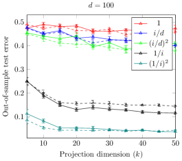
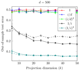
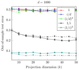
Figure 1: Out-of-sample error of $1$-NN on synthetic data sets, with metric learning (solid lines), and without metric learning (dashed lines), averaged over $10$ Gaussian random projections, for several choices of $d$, and $s({\mathcal{X}})$. The data support was $\mathcal{X}=A{\mathcal{S}}^{d-1}$, where $A\in\mathbb{R}^{d\times d}$ is a diagonal matrix, and the legend shows its $i$-th diagonal element, for $i\in[d]$. The curves represent averages over $10$ independent Gaussian random projections. The error bars show intervals of one standard error.

Figure 1 shows the empirical results obtained. As expected from the theory, we see that the error is affected by the stable dimension, which, in turn, depends on the rate of decay on the eigenvalues of $A$ (shown in the legends), and is unaffected by the ambient dimension. To confirm, we repeated these experiments with different values of $d$, and for different decay rates on the eigenvalues of $A$. We can see that going from $d=100$ to $d=500$, incurs a small increase in the error, for all decay rates. This is because $s(\mathcal{X})$ increases considerably, when that decay is not small enough, and so does the error. When going from $d=500$ to $d=1000$, however, all rates of decay, retain about the same error, as only small eigenvalues are added, and $s(\mathcal{X})$ increases only slightly. This observation, of course, does not consider the small fluctuations, that result from the randomness of the compression.

In addition, comparing the solid and dashed lines in Figure 1, we see that metric learning appears to be useful even for small values of $k$, provided $s(\mathcal{X})$ is small. While it is expected that random compression makes the covariance of the data distribution more “spherical”, and can potentially distort any separation that existed, if the support is highly anisotropic, i.e., $s(\mathcal{X})$ is low, then the separability can still be preserved to a high degree. Thus, a learnt metric can still outperform the classic Euclidean metric. Indeed, we can see that, in the $(1/i)$-case, the dashed lines diverge from the respective solid lines, as $k$ increases. An exception to the above is when $s(\mathcal{X})$ is too small, and the empirical error without metric learning is already low, so learning a metric does not significantly improve it.

3.2 Experiments with benchmark data sets

Benchmark data sets will serve to test the usefulness and effectiveness of metric learning under compression in a more general context, and its adaptability to noisy settings. In real data, the value of the stable dimension of the support is unknown, but one may expect some structure that metric learning can exploit. We follow the same experimental protocol as in synthetic data sets (80%/20% split), and compute the empirical error, for varying degrees of compression. We want to test if the trade-off can be minimised by some value of $k$.

Our test experiments are somewhat inspired from the evaluation idea in [1], where noise features were appended to low-dimensional data to test the abilities of metric learning. We start from three benchmark UCI data sets with moderate ambient dimension from [16]: Ionosphere (2 labels, 33 features, 351 instances), Wine (3 labels, 13 features, 178 instances), and Sonar (2 labels, 60 features, 208 instances). For each set, we normalised its features to $[0,1]$, embedded it onto a higher-dimensional ambient space, and added some Gaussian noise to all features and all instances, with variance $\gamma$. This simulates the “noisy subspace hypothesis”, in which the data cluster in a noisy low-dimensional subspace in the ambient space [17, Section 1.1].

We aim to test whether Gaussian random projection is still able to preserve information from the features that span the underlying subspace. We also repeated the experiments for different values of $\gamma$, to test how easily metric learning can adapt in each case. In the Appendix, we repeat these experiments for different compression schemes, to draw comparisons with the Gaussian.

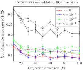
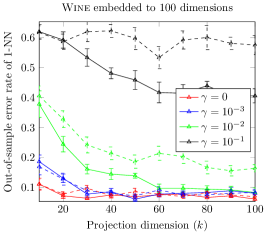
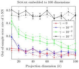
Figure 2: Out-of-sample error of $1$-NN classification with metric learning (solid lines) and with Euclidean metric (dashed lines), of benchmark UCI data sets. All data sets were normalised to $[0,1]$, embedded to a $100$-dimensions, and had i.i.d. Gaussian random noise of variance $\gamma$ (shown in the legend) added to each of their instances. A train/test ratio of $80\%/20\%$ was used. The curves represent averages over $10$ independent Gaussian random projections. The error bars show intervals of one standard error.

Figure 2 shows the results. As we can see, the higher the noise variance $\gamma$, the higher the average error incurred by the algorithm. However, in almost all cases, there seems to be a lower bound for $k$, above which the performance stops increasing significantly. This means that the trade-off between accuracy and complexity can be minimised, by choosing that value of $k$ (e.g. by employing cross-validation type procedures). In the Appendix, we revisit this setting, for higher-dimensional embeddings.

Regarding the performance of metric learning, compared to the Euclidean metric, it is not straightforward to draw any conclusions, because it depends on the unknown structure of the data and the available sample size, although in the higher-noise regime we see a consistently outperformance from learning the metric.

4 Related work

Mahalanobis metric learning was introduced in [2] and has attracted a significant amount of research since. Shortly after its introduction, two of the most popular metric learning algorithms were proposed; Large Margin Nearest Neighbour (LMNN) [3], and Information Theoretic Metric Learning (ITML) [4]. Generalisations and extensions to metric learning algorithms have also been well-studied. We refer the reader to the surveys in [18, 19] for a more detailed review on metric learning algorithms. There have also been attempts to learn non-linear metrics (e.g. [20, 21]), as well as to train neural networks in metric learning, known as deep metric learning (see [22] for a survey). Metric learning has also been applied to other fields, e.g. collaborative filtering [23], and facial recognition [24].

Much recent literature has been devoted to mitigate the undesirable effects of the curse of dimensionality on metric learning. A typical approach is to train a low-dimensional metric in the ambient space, this was demonstrated to improve the classification performance – see e.g. [25] and the references therein.

A notable thread of research, which our work builds upon, appears in a NeurIPS paper [1]. The authors consider both distance-based and classifier-based Mahalanobis metric learning, and show that in general its sample complexity necessarily grows with the dimension of the features in the data, unless a Frobenius norm-constraint is imposed onto the hypothesis class of Mahalanobis metrics, in which case a smaller sample size is required, for a low generalisation error – provided that the problem admits such constraint. Because the optimal constraint is not known in advance, their choice of Frobenius norm-constraint is somewhat arbitrary. In a closely related model, namely a quadratic classifier class, [26] found the nuclear-norm constraint leads to the ability of the error to adapt to a notion of intrinsic dimension of the data (the effective rank of the true covariance), while the Frobenius norm constraint was shown to lack such ability. Their bound still has a mild logarithmic dependence on the ambient dimension.

All of the above methods (and most others) work with the full data set, which can be limiting with high-dimensional data. In real-world high-dimensional settings, it is common to only have access to a compressed version of the original features. This can be either due to space constraints, or because a lower-dimensional data set is easier to work with from a computational point of view. Learning from, or reconstructing compressed observations, has been well-studied in the literature, in a field known as compressed sensing [27]. In fact, the geometric structures that make compressed sensing easier have also been examined in the analysis of learning tasks to some extent, e.g. [9]. Novel data acquisition sensors from compressed sensing enable collecting data in a randomly compressed form, alleviating the need to select and discard significant fractions of it during pre-processing [28].

In this work we only assumed to have access to an already compressed version of the original data and never need the original. Yet, the guarantees we provide are relative to the original high-dimensional parameters. To the best of our knowledge, distance-based metric learning has eluded a systematic study under compression so far. This paper aims to lessen this gap between theory and practice, and quantify the extra loss we suffer from the random compression, as well as identify the conditions that reduce that loss.

5 CONCLUSIONS AND FUTURE WORK

We considered Mahalanobis metric learning when working with a randomly compressed version of the data. We derived high-probability theoretical guarantees for its generalisation error, as well as for its excess empirical error under Gaussian random projection. We showed theoretically that both quantities are unaffected by the ambient dimension, and instead depend on the stable dimension of the data support. We supported these findings with experiments on both synthetic and benchmark data sets in conjunction with Nearest Neighbour classification, using its empirical performance to evaluate the learnt metric learning.

In this work we only considered properties of the support of the data. Future work may focus on effects from other distributional traits. This may be particularly useful in settings where the covariance of the distribution is far from isotropic, and the data support is only bounded with high-probability. Related work has been done for quadratic classifiers in [26], which showed that the effective rank of the covariance matrix (a measure of ID) affects the generalisation error. The second-moment matrix is usually unknown, so it would be insightful to see how metric learning can automatically adapt to some particular structure in that matrix.

Another possible extension is to study the setting where each compressed instance is perturbed by random noise. Metric learning under noisy regimes has already been examined, e.g. [29], but only for the ambient space. Considering the effect of noise on metric learning under compression may also be of interest in many real-world settings.

Appendix A PROOFS OF THEORETICAL RESULTS

A.1 Proof of Lemma 4

To prove Lemma 4, we first recall a well-known inequalitiy regarding Gaussian processes (see [14, Section 7.3] and the references therein for the definitions and derivations).

Lemma 9 (Sudakov-Fernique’s inequality [14, Theorem 7.2.11]).

Let $(X_{t})_{t\in T}$ and $(Y_{t})_{t\in T}$ be two mean-zero Gaussian processes and assume that for all $t,s\in T$, we have

$$\mathop{{}\mathbb{E}}(X_{t}-X_{s})^{2}\leq\mathop{{}\mathbb{E}}(Y_{t}-Y_{s})^{2}.$$ (17)

Then, we have

$$\mathop{{}\mathbb{E}}\sup_{t\in T}X_{t}\leq\mathop{{}\mathbb{E}}\sup_{t\in T}Y_{t}.$$ (18)

Equipped with Lemma 9, we are now ready for the proof of Lemma 4. We first define two mean-zero Gaussian processes as

$$X_{u,x}:=bg^{\top}u+h^{\top}x\qquad\text{ and }\qquad Y_{u,x}:=u^{\top}Rx$$ (19)

where $(u,x)\in\mathcal{S}^{k-1}\times T$ and $g\sim\mathcal{N}(0_{k},I_{k})$ and $h\sim\mathcal{N}(0_{d},I_{d})$ are independent from each other.

For all $(u,x),(u^{\prime},x^{\prime})\in\mathcal{S}^{k-1}\times T$, we have

$$\mathop{{}\mathbb{E}}|X_{u,x}-X_{u^{\prime},x^{\prime}}|^{2} =\mathop{{}\mathbb{E}}(bg^{\top}u+h^{\top}x-bg^{\top}u^{\prime}-h^{\top}x^{\prime})^{2}$$ (20)

$$=2b^{2}-2b^{2}u^{\top}u^{\prime}+\|x\|^{2}+\|x^{\prime}\|^{2}-2x^{\top}x^{\prime},$$ (21)

and

$$\mathop{{}\mathbb{E}}|Y_{u,x}-Y_{u^{\prime},x^{\prime}}|^{2} =\mathop{{}\mathbb{E}}(u^{\top}Rx-u^{\prime\top}Rx^{\prime})^{2}$$ (22)

$$=\mathop{{}\mathbb{E}}\left(\sum_{i=1}^{k}\sum_{j=1}^{d}(R)_{ij}(u_{i}x_{j}-u^{\prime}_{i}x^{\prime}_{j})\right)^{2}$$ (23)

$$=\sum_{i=1}^{k}\sum_{j=1}^{d}(u_{i}x_{j}-u^{\prime}_{i}x^{\prime}_{j})^{2}$$ (24)

$$=\|ux^{\top}-u^{\prime}x^{\prime\top}\|_{F}^{2}$$ (25)

$$=\operatorname{tr}((ux^{\top}-u^{\prime}x^{\prime\top})^{\top}(ux^{\top}-u^{\prime}x^{\prime\top}))$$ (26)

$$=\operatorname{tr}(xu^{\top}ux^{\top})+\operatorname{tr}(x^{\prime}u^{\prime\top}u^{\prime}x^{\prime\top})-2\operatorname{tr}(x^{\prime}u^{\prime\top}ux^{\top})$$ (27)

$$=\operatorname{tr}(x^{\top}x)+\operatorname{tr}(x^{\prime\top}x^{\prime})-2\operatorname{tr}(u^{\top}u^{\prime})\operatorname{tr}(x^{\top}x^{\prime})$$ (28)

$$=\|x\|^{2}+\|x^{\prime}\|^{2}-2(u^{\top}u^{\prime})(x^{\top}x^{\prime}).$$ (29)

Therefore, we find that

$$\mathop{{}\mathbb{E}}|X_{u,x}-X_{u^{\prime},x^{\prime}}|^{2}-\mathop{{}\mathbb{E}}|Y_{u,x}-Y_{u^{\prime},x^{\prime}}|^{2}=2(1-u^{\top}u^{\prime})(b^{2}-x^{\top}x^{\prime}).$$ (30)

This means that for all $(u,x),(u^{\prime},x^{\prime})\in\mathcal{S}^{k-1}\times T$ we have

$$\mathop{{}\mathbb{E}}|X_{u,x}-X_{u^{\prime},x^{\prime}}|^{2}-\mathop{{}\mathbb{E}}|Y_{u,x}-Y_{u^{\prime},x^{\prime}}|^{2}\geq 0.$$ (31)

Therefore, the conditions of Lemma 9 are satisfied, and thus

$$\mathop{{}\mathbb{E}}\sup_{(u,x)\in\mathcal{S}^{k-1}\times T}X_{u,x}\geq\mathop{{}\mathbb{E}}\sup_{(u,x)\in\mathcal{S}^{k-1}\times T}Y_{u,x}.$$ (32)

Noting that

$$\mathop{{}\mathbb{E}}\sup_{u\in\mathcal{S}^{k-1}}\sup_{x\in T}X_{u,x}=b\mathop{{}\mathbb{E}}\sup_{u\in\mathcal{S}^{k-1}}g^{\top}u+\mathop{{}\mathbb{E}}\sup_{x\in T}h^{\top}x=ba(k)+\omega(T).$$ (33)

and

$$\mathop{{}\mathbb{E}}\sup_{u\in\mathcal{S}^{k-1}}\sup_{x\in T}Y_{u,x}=\mathop{{}\mathbb{E}}\sup_{u\in\mathcal{S}^{k-1}}\sup_{x\in T}u^{\top}Rx=\mathop{{}\mathbb{E}}\sup_{x\in T}\|Rx\|$$ (34)

we conclude that

$$\mathop{{}\mathbb{E}}\sup_{x\in T}\|Rx\|\leq ba(k)+\omega(T).$$ (35)

It remains to bound $\sup_{x\in T}\|Rx\|$ with high-probability away from its expectation. To this end, we claim that the function $f(R)=\sup_{x\in T}\|Rx\|$ is $b$-Lipschitz with respect to the Euclidean norm. To see why, let $R_{1},R_{2}\in\mathbb{R}^{k\times d}$ be fixed matrices (which can also be seen as vectors in $\mathbb{R}^{kd}$), and note that

$$|f(R_{1})-f(R_{2})| =|\sup_{x\in T}\|R_{1}x\|-\sup_{x\in T}\|R_{2}x\||$$ (36)

$$\leq\sup_{x\in T}|\|R_{1}x\|-\|R_{2}x\||$$ (37)

$$\leq\sup_{x\in T}\|(R_{1}-R_{2})x\|$$ (38)

$$\leq\sup_{x\in T}\|x\|\sigma_{\max}(R_{1}-R_{2})$$ (39)

$$=b\sigma_{\max}(R_{1}-R_{2})$$ (40)

$$\leq b\|R_{1}-R_{2}\|_{F}.$$ (41)

Invoking the upper bound of [30, Theorem 2.26], we complete the proof.

A.2 Proof of Theorem 5

Let $\mathcal{P}$ be a probability measure induced by the random variable $(X,Y)$, where $X:=(x,x^{\prime})$ and $Y:=\mathbf{1}\{y=y^{\prime}\}$, for $((x,y),(x^{\prime},y^{\prime}))\sim\mathcal{D}^{2}$. Also denote $\mathcal{D}_{\mathcal{X}}$ the marginal distribution induced by $\mathcal{D}$ on $\mathcal{X}$. Also let $\ell_{l,u}$ be the loss function defined in (4). Given a matrix $R$, we define the function class in the compressed space as

$$\mathcal{F}_{R}=\{f_{M}:(x_{1},x_{2})\to\|M(Rx_{1}-Rx_{2})\|^{2}:M\in\mathcal{M}_{k}\text{ and }x_{1},x_{2}\in\mathcal{X}\}.$$ (42)

Also, for all $i\in[n]$, let $X_{i}:=(x_{2i-1},x_{2i})$ and $Y_{i}:=\mathbf{1}\{y_{2i-1},y_{2i}\}$ be “regrouped” versions of the elements of $T$, defined in (3). We are interested in upper bounding

$$\sup_{f_{M}\in\mathcal{F}_{R}}\left(\mathop{{}\mathbb{E}}_{(X,Y)\sim\mathcal{P}}\ell_{l,u}(f_{M}(X),Y)-\frac{1}{n}\sum_{i=1}^{n}\ell_{l,u}(f_{M}(X_{i}),Y_{i})\right)$$ (43)

We then upper bound the Rademacher complexity of $\mathcal{F}_{R}$, with respect to $\mathcal{P}$. Let $\sigma_{1},\ldots,\sigma_{n}$ be i.i.d. uniform $\{\pm 1\}$-valued random variables. Modifying the proof of [1, Theorem 1], we obtain with probability at least $1-\epsilon$

$$\mathcal{R}_{n,\mathcal{D}}(\mathcal{F}_{R}) :=\frac{1}{n}\mathop{{}\mathbb{E}}_{\begin{subarray}{c}\sigma_{i},X_{i}\\ i\in[n]\end{subarray}}\sup_{f_{M}\in\mathcal{F}_{R}}\sum_{i=1}^{n}\sigma_{i}f_{M}(x_{2i-1},x_{2i})$$ (44)

$$=\frac{1}{n}\mathop{{}\mathbb{E}}_{\begin{subarray}{c}\sigma_{i},X_{i}\\ i\in[n]\end{subarray}}\sup_{M\in\mathcal{M}_{k}}\sum_{i=1}^{n}\sigma_{i}(x_{2i-1}-x_{2i})^{\top}R^{\top}M^{\top}MR(x_{2i-1}-x_{2i})$$ (45)

$$\leq\frac{1}{\sqrt{n}}\sup_{M\in\mathcal{M}_{k}}\|M^{\top}M\|_{F}(\mathop{{}\mathbb{E}}_{(x,x^{\prime})\sim\mathcal{D}_{\mathcal{X}}\times\mathcal{D}_{\mathcal{X}}}\|R(x-x^{\prime})\|^{4})^{1/2}$$ (46)

$$\leq\frac{\sqrt{k}}{\sqrt{n}\operatorname{diam}(\mathcal{X})^{2}}(\mathop{{}\mathbb{E}}_{(x,x^{\prime})\sim\mathcal{D}_{\mathcal{X}}\times\mathcal{D}_{\mathcal{X}}}\|R(x-x^{\prime})\|^{4})^{1/2}$$ (47)

$$\leq\frac{\sqrt{k}}{\sqrt{n}\operatorname{diam}(\mathcal{X})^{2}}\sup_{x,x^{\prime}\in\mathcal{X}}\|R(x-x^{\prime})\|^{2}$$ (48)

$$\leq\frac{\sqrt{k}}{\sqrt{n}\operatorname{diam}(\mathcal{X})^{2}}\left(\operatorname{diam}(\mathcal{X})+\frac{\omega(\mathcal{X}-\mathcal{X})}{\sqrt{k}}+\operatorname{diam}(\mathcal{X})\sqrt{\frac{2\ln\frac{1}{\epsilon}}{k}}\right)^{2}$$ (49)

$$\leq\frac{\sqrt{k}}{\sqrt{n}\operatorname{diam}(\mathcal{X})^{2}}\left(\operatorname{diam}(\mathcal{X})+\frac{\psi(\mathcal{X}-\mathcal{X})}{\sqrt{k}}+\operatorname{diam}(\mathcal{X})\sqrt{\frac{2\ln\frac{1}{\epsilon}}{k}}\right)^{2}$$ (50)

$$=\sqrt{\frac{k}{n}}\left(1+\sqrt{\frac{s(\mathcal{X})}{k}}+\sqrt{\frac{2\ln\frac{1}{\epsilon}}{k}}\right)^{2}.$$ (51)

We used the upper bound of Lemma 4 to obtain (49), and the inequality of Lemma 3 to obtain (50). To complete the proof, we then invoke the well-known Rademacher bound, which we include for completeness in the following lemma, combined with the union bound [31, Theorem 1.2.11.b].

Lemma 10 (Rademacher bound [32]).

Let $\mathcal{D}$ be a distribution over $\mathcal{X}\times\{-1,1\}$ and let $\{(x_{i},y_{i})\}_{i=1}^{n}$ be a sample of size $n$ drawn i.i.d. from $\mathcal{D}$. Given a hypothesis class $\mathcal{F}$ and a loss function $\ell:\mathbb{R}\times\{-1,1\}\to\mathbb{R}$ such that $|\ell(y^{\prime},y)|\leq 1$, for all $y^{\prime},y\in\mathbb{R}$ and $\ell$ is $\rho$-Lipschitz in its first argument, then, for any $0<\epsilon<1$, with probability at least $1-\epsilon$ for all $f\in\mathcal{F}$, we have

$$\mathop{{}\mathbb{E}}_{(x,y)\sim\mathcal{D}}\ell(f(x),y)\leq\frac{1}{n}\sum_{i=1}^{n}\ell(f(x_{i}),y_{i})+2\rho\mathcal{R}_{n,\mathcal{D}}(\mathcal{F})+\sqrt{\frac{\ln\frac{1}{\epsilon}}{2n}}$$ (52)

where $\mathcal{R}_{n,\mathcal{D}}(\mathcal{F})$ is the Rademacher complexity of the hypothesis class $\mathcal{F}$, given a sample of size $n$ i.i.d. from $\mathcal{D}$, and is defined as

$$\mathcal{R}_{n,\mathcal{D}}(\mathcal{F}):=\frac{1}{n}\mathop{{}\mathbb{E}}_{\sigma}\sup_{f\in\mathcal{F}}\sum_{i=1}^{n}\sigma_{i}f(x_{i})$$ (53)

where $\sigma:=\begin{bmatrix}\sigma_{1},\ldots,\sigma_{n}\end{bmatrix}^{\top}$ is a random vector, consisting of $n$, i.i.d., uniform, $\{\pm 1\}$-valued random variables.

A.3 Proof of Theorem 7

Consider any pair of hypotheses, $M\in\mathcal{M}_{k}$, and $M_{0}\in\mathcal{M}$. Using the $\rho$-Lipschitz property of $\ell_{l,u}$, we have

$$\hat{L}^{R}_{T}(M)-\hat{L}_{T}(M_{0})\leq\frac{\rho}{n}\sum_{i=1}^{n}|\|MR(x_{2i-1}-x_{2i})\|^{2}-\|M_{0}(x_{2i-1}-x_{2i})\|^{2}|.$$ (54)

To upper bound the absolute value in (54), we need to both lower and upper bound the quantity inside, with respect to $R$, and take the maximum of the two. There are two terms inside the maximum, which must be lower and upper bounded separately.

For the first term, recall that $\sigma_{\max}(M)=\sigma_{\max}(M_{0})=1/\operatorname{diam}(\mathcal{X})$ by their definition. We invoke Lemma 3 and both bounds of Lemma 4 to obtain our results. For the upper bound, with probability at least $1-\epsilon$, we have for all $i\in[n]$

$$\|MR(x_{2i-1}-x_{2i})\| \leq\sigma_{\max}(M)\|R(x_{2i-1}-x_{2i})\|$$ (55)

$$\leq\frac{1}{\operatorname{diam}(\mathcal{X})}\|R(x_{2i-1}-x_{2i})\|$$ (56)

$$\leq\frac{1}{\operatorname{diam}(\mathcal{X})}\sup_{x,x^{\prime}\in\mathcal{X}}\|R(x-x^{\prime})\|$$ (57)

$$\leq 1+\sqrt{\frac{s(\mathcal{X})}{k}}+\sqrt{\frac{2\ln\frac{1}{\epsilon}}{k}}.$$ (58)

For the lower bound, with probability at least $1-\epsilon$, we have for all $i\in[n]$

$$\|MR(x_{2i-1}-x_{2i})\|\geq 0.$$ (59)

For the second term, since $\sigma_{\max}(M_{0})=1/\operatorname{diam}(\mathcal{X})$, we have for all $i\in[n]$

$$0\leq\|M_{0}(x_{2i-1}-x_{2i})\|^{2}\leq 1.$$ (60)

Plugging the lower and upper bounds into (54), we obtain, with probability at least $1-\epsilon$

$$\hat{L}^{R}_{T}(M)-\hat{L}_{T}(M_{0})\leq\max\left\{\rho\left(1+\sqrt{\frac{s(\mathcal{X})}{k}}+\sqrt{\frac{2\ln\frac{1}{\epsilon}}{k}}\right)^{2},\rho\right\}.$$ (61)

Since the first term inside the maximum is always greater than $\rho$, this simplifies to our desired result.

Appendix B EXPERIMENTAL DETAILS

In this section we outline the details of the experiments reported in Section 3. We detail the algorithmic steps that we followed to obtain the results, as well as our method of choosing the embedding and adding noise to a data set.

B.1 Algorithm

The formal steps of the experimental process are outlined in Algorithm 1.

Input: $T:=\{(x_{i},y_{i})\}_{i=1}^{n}$: original data set, $k$: projection dimension, $t$: number of random projections.

Output: $a_{1}$: average out-of-sample average error of $1$-NN with metric, $a_{2}$: average out-of-sample error of $1$-NN without metric.

1 Randomly partition $T$ into $T_{1}$ and $T_{2}$ (i.e. $T_{1}\cup T_{2}=T$, and $T_{1}\cap T_{2}=\emptyset$), and $|T_{1}|=4|T_{2}|$;

2 Set $a_{1},a_{2}\leftarrow 0$;

3 for $j\in[t]$ do

4       Sample $R\in\mathbb{R}^{k\times d}$ with elements i.i.d. from $\mathcal{N}(0,1/k)$;

5       Compress $T_{1}$ and $T_{2}$ to obtain $RT_{1}:=\{(Rx,y):(x,y)\in T_{1}\}$ and $RT_{2}:=\{(Rx,y):(x,y)\in T_{2}\}$;

6       Run LMNN on the set $RT_{1}$ and record the output metric as $M\in\mathbb{R}^{k\times k}$;

7       Run $1$-NN under the metric $M$, to classify the set $RT_{2}$, using $RT_{1}$ for reference instances, and record its classification error as $b_{1}\in[0,1]$;

8       Run $1$-NN under the metric $I_{k}$, to classify the set $RT_{2}$, using $RT_{1}$ for reference instances, and record its classification error as $b_{2}\in[0,1]$;

9       Update $a_{1}\leftarrow a_{1}+b_{1}/t$;

10       Update $a_{2}\leftarrow a_{2}+b_{2}/t$;

return $a_{1}$, $a_{2}$.

Algorithm 1 Calculation of average out-of-sample error, from multiple random projections.

For the experiments we used the R programming language. To train the metric with LMNN in algorithm 1, we used the function mlpack::lmnn by accepting the defaults for all parameters.

B.2 Simulating a noisy subspace structure

We sample a random semi-orthogonal matrix $A\in\mathbb{R}^{N\times n}$, i.e. $A^{\top}A=I_{n}$, and use this to embed each data set $T\in\mathbb{R}^{n}$ into the higher-dimensional space $\mathbb{R}^{N}$, where $n<N$. We then use the set $AT$ as the input to the Mahalanobis metric learning algorithm. This ensures that the original structure, including distances between vectors, is perfectly preserved.

To add Gaussian random noise to the set $AT\subset\mathbb{R}^{N}$, we fix the noise variance, denote $\gamma$, and add a Gaussian random vector, $g\sim\mathcal{N}(0_{N},\gamma I_{N})$, to each vector of $AT$, where $g$ is sampled i.i.d. for each vector of $AT$. This does not change the number of points of the set, nor its embedding dimension, but it changes its stable dimension (see Definition 2), so this allows us to control the stable dimension in our experiments.

Appendix C ADDITIONAL EXPERIMENTS

Our theoretical results assumed the RP matrix, $R$, to be Gaussian with i.i.d. entries, as we leveraged proof techniques that are specific to the Gaussian (i.e. the comparison inequalities for Gaussian processes). Our aim in this section is to test the robustness of our findings with respect to departures from the Gaussian assumption on $R$. While the choice of $R$ rests with the user, or the data sensing/collection device, different RP matrices are in use in practice for their computational advantages.

To this end, we performed additional experiments on synthetic and benchmark data sets, with different RP matrices, and higher embedding dimensions, to compare with the experiments reported in Section 3. The choices for RP were made to satisfy the Johnson-Lindenstrauss (JL) property [33], which means that, for all pairs of points $(x_{i},x_{j})$ in a finite set $T$, with high-probability (exponentially decreasing in $\epsilon^{2}$), we have

$$(1-\epsilon)\|x_{i}-x_{j}\|^{2}\leq\|Rx_{i}-Rx_{j}\|^{2}\leq(1+\epsilon)\|x_{i}-x_{j}\|^{2}.$$ (62)

provided the target projection dimension is of order logarithmic in $|T|$. Extensions that allow for infinite sets $T$ exist for Gaussian and sub-gaussian RP matrices [11], [14, Sec. 9.1].

The projections we used are

• JL with binary coins [8];

• fast JL transform [34]; and

• circulant transform [35].

All these types of compression satisfy some form of the JL property in (62), and we refer the interested reader to the corresponding citations, given above, for further details on each. Besides this change, we followed the same steps outlined in Algorithm 1, only changing algorithm 1, according to the type of compression that we use.

C.1 Additional experiments with synthetic sets

We reconsider the synthetic sets used in Section 3.1, and conduct more experiments using different RP matrices, to verify if they behave similarly to the Gaussian RP that we had in Figure 1.

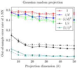
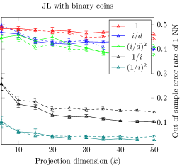
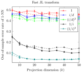
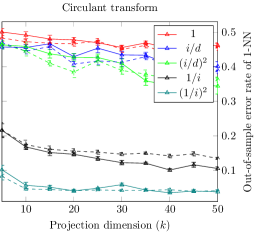
Figure 3: Out-of-sample error of $1$-NN on $100$-dimensional synthetic data sets, with metric learning (solid lines), and without metric learning (dashed lines), averaged over $10$ independent compressions. Four different compression schemes were used, as shown in the titles. The data support was $\mathcal{X}=A{\mathcal{S}}^{d-1}$, where $A\in\mathbb{R}^{d\times d}$ is a diagonal matrix, and the legend shows its $i$-th diagonal element, for $i\in[d]$.

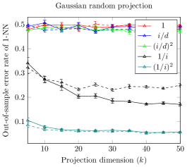
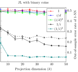
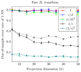
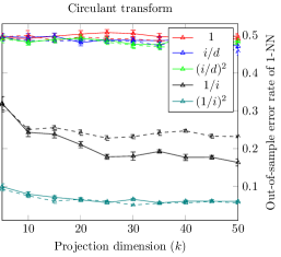
Figure 4: Out-of-sample error of $1$-NN on $500$-dimensional synthetic data sets, with metric learning (solid lines), and without metric learning (dashed lines), averaged over $10$ independent compressions. Four different compression schemes were used, as shown in the titles. The data support was $\mathcal{X}=A{\mathcal{S}}^{d-1}$, where $A\in\mathbb{R}^{d\times d}$ is a diagonal matrix, and the legend shows its $i$-th diagonal element, for $i\in[d]$.

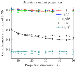
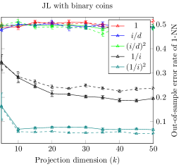
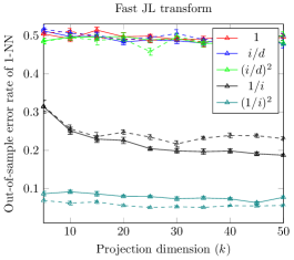
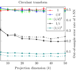
Figure 5: Out-of-sample error of $1$-NN on $1000$-dimensional synthetic data sets, with metric learning (solid lines), and without metric learning (dashed lines), averaged over $10$ independent compressions. Four different compression schemes were used, as shown in the titles. The data support was $\mathcal{X}=A{\mathcal{S}}^{d-1}$, where $A\in\mathbb{R}^{d\times d}$ is a diagonal matrix, and the legend shows its $i$-th diagonal element, for $i\in[d]$.

Figures 3, 4 and 5 present the results. We can clearly see that Gaussian random projection performs very similarly with the three other compression types we used. This similar behaviour is observed for all values of $d$. Therefore, the observation that the stable dimension of the data support appears to influence the error, carries over to these types of projection as well.

C.2 Additional experiments with benchmark data sets

For experiments with real data, we reconsider the benchmark UCI sets used in Section 3.2. We embedded them to $100$, $250$, and $500$ dimensions, and we experimented with different RP matrices to compare with Figure 2. The primary purpose of these experiments, as in Section 3.2, is to examine whether the ambient dimension plays any role in the performance of the algorithm when the stable dimension stays the same. In addition, here we want to see if the non-gaussian RPs behave similarly to what we observed with Gaussian RP in Section 3.2.

A data set embedded in higher-dimensions will maintain the same stable dimension, as long as no noise is added afterwards. However, the more noise we add, the more likely that the stable dimension increases. We therefore want to also test the effect of noise in these settings, and see how they complement our theory.

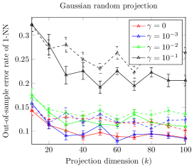
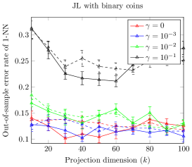
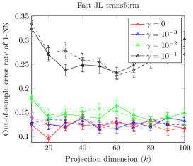
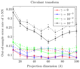
Figure 6: Out-of-sample error of $1$-NN classification with metric learning (solid lines) and with Euclidean metric (dashed lines), of UCI data set Ionosphere. The original data set was normalised to $[0,1]$, embedded onto $100$-dimensions, and had i.i.d. Gaussian random noise of variance $\gamma$ (shown in the legend) added to each of its instances. A train/test ratio of $80\%/20\%$ was used. The curves represent averages over $10$ independent compressions. The error bars show intervals of one standard error. Four different compression schemes were used, as shown in the titles.

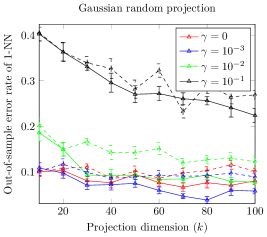
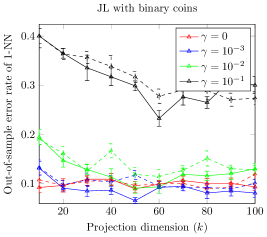
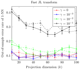
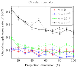
Figure 7: Out-of-sample error of $1$-NN classification with metric learning (solid lines) and with Euclidean metric (dashed lines), of UCI data set Ionosphere. The original data set was normalised to $[0,1]$, embedded onto $250$-dimensions, and had i.i.d. Gaussian random noise of variance $\gamma$ (shown in the legend) added to each of its instances. A train/test ratio of $80\%/20\%$ was used. The curves represent averages over $10$ independent compressions. The error bars show intervals of one standard error. Four different compression schemes were used, as shown in the titles.

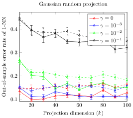
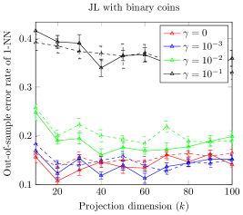
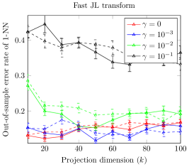
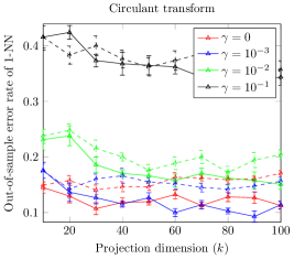
Figure 8: Out-of-sample error of $1$-NN classification with metric learning (solid lines) and with Euclidean metric (dashed lines), of UCI data set Ionosphere. The original data set was normalised to $[0,1]$, embedded onto $500$-dimensions, and had i.i.d. Gaussian random noise of variance $\gamma$ (shown in the legend) added to each of its instances. A train/test ratio of $80\%/20\%$ was used. The curves represent averages over $10$ independent compressions. The error bars show intervals of one standard error. Four different compression schemes were used, as shown in the titles.

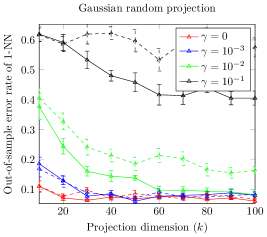
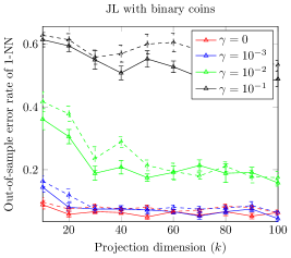
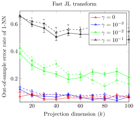
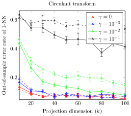
Figure 9: Out-of-sample error of $1$-NN classification with metric learning (solid lines) and with Euclidean metric (dashed lines), of UCI data set Wine. The original data set was normalised to $[0,1]$, embedded onto $100$-dimensions, and had i.i.d. Gaussian random noise of variance $\gamma$ (shown in the legend) added to each of its instances. A train/test ratio of $80\%/20\%$ was used. The curves represent averages over $10$ independent compressions. The error bars show intervals of one standard error. Four different compression schemes were used, as shown in the titles.

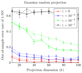
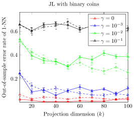
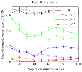
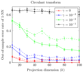
Figure 10: Out-of-sample error of $1$-NN classification with metric learning (solid lines) and with Euclidean metric (dashed lines), of UCI data set Wine. The original data set was normalised to $[0,1]$, embedded onto $250$-dimensions, and had i.i.d. Gaussian random noise of variance $\gamma$ (shown in the legend) added to each of its instances. A train/test ratio of $80\%/20\%$ was used. The curves represent averages over $10$ independent compressions. The error bars show intervals of one standard error. Four different compression schemes were used, as shown in the titles.

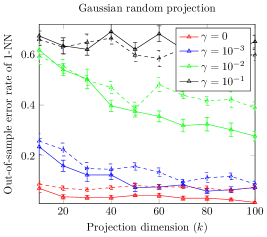
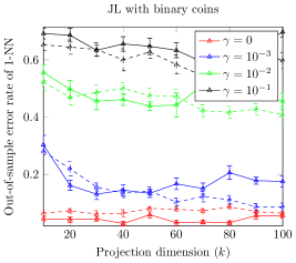
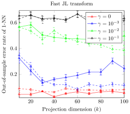
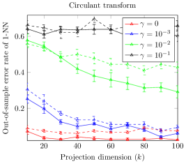
Figure 11: Out-of-sample error of $1$-NN classification with metric learning (solid lines) and with Euclidean metric (dashed lines), of UCI data set Wine. The original data set was normalised to $[0,1]$, embedded onto $500$-dimensions, and had i.i.d. Gaussian random noise of variance $\gamma$ (shown in the legend) added to each of its instances. A train/test ratio of $80\%/20\%$ was used. The curves represent averages over $10$ independent compressions. The error bars show intervals of one standard error. Four different compression schemes were used, as shown in the titles.

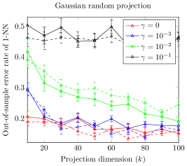
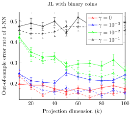
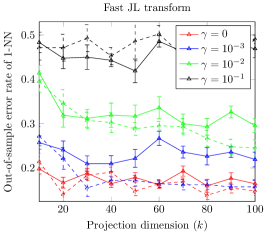
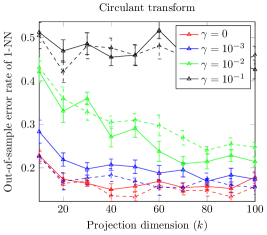
Figure 12: Out-of-sample error of $1$-NN classification with metric learning (solid lines) and with Euclidean metric (dashed lines), of UCI data set Sonar. The original data set was normalised to $[0,1]$, embedded onto $100$-dimensions, and had i.i.d. Gaussian random noise of variance $\gamma$ (shown in the legend) added to each of its instances. A train/test ratio of $80\%/20\%$ was used. The curves represent averages over $10$ independent compressions. The error bars show intervals of one standard error. Four different compression schemes were used, as shown in the titles.

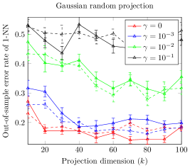
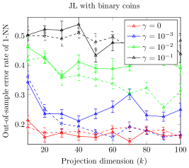
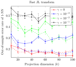
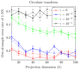
Figure 13: Out-of-sample error of $1$-NN classification with metric learning (solid lines) and with Euclidean metric (dashed lines), of UCI data set Sonar. The original data set was normalised to $[0,1]$, embedded onto $250$-dimensions, and had i.i.d. Gaussian random noise of variance $\gamma$ (shown in the legend) added to each of its instances. A train/test ratio of $80\%/20\%$ was used. The curves represent averages over $10$ independent compressions. The error bars show intervals of one standard error. Four different compression schemes were used, as shown in the titles.

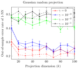
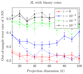
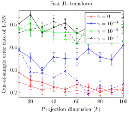
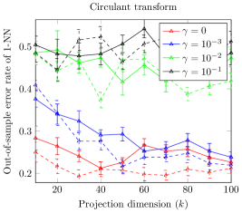
Figure 14: Out-of-sample error of $1$-NN classification with metric learning (solid lines) and with Euclidean metric (dashed lines), of UCI data set Sonar. The original data set was normalised to $[0,1]$, embedded onto $500$-dimensions, and had i.i.d. Gaussian random noise of variance $\gamma$ (shown in the legend) added to each of its instances. A train/test ratio of $80\%/20\%$ was used. The curves represent averages over $10$ independent compressions. The error bars show intervals of one standard error. Four different compression schemes were used, as shown in the titles.

Figures 6 and 14 present the results. As in the synthetic setting, different RP matrices produce very similar results as the Gaussian RP.

In addition, for most cases there appears to be an upper bound on $k$, above which the error stops decreasing. This, again, signifies that a potential minimisation of the trade-off between accuracy and complexity is possible, by appropriately choosing the value of $k$.

In almost all simulations, metric learning outperforms the Euclidean metric in large-noise settings. When the noise is smaller, metric learning is on par with, and can even produce higher error than the Euclidean metric. Of course, one cannot draw conclusions with certainty, as results are data-dependent, and there is also considerable fluctuation stemming from the randomness of the compression.

Regarding the choice of the embedding dimension for the same set, it appears that a higher value can increase the error, when the magnitude of the noise is large. This is probably a consequence of the fact that Gaussian random vectors in higher-dimensions, tends to have a higher expected norm, than in lower dimensions [14, Section 3.1]. Therefore, the added Gaussian noise, tends to augment the stable dimension more in higher dimensions than in lower dimensions, thus causing the observed deterioration, in agreement with our theory. It should be noted that Ionosphere seems much more resistant to added noise, than Wine and Sonar.

References

- [1] Nakul Verma and Kristin Branson. Sample complexity of learning Mahalanobis distance metrics. Advances in neural information processing systems, 28, 2015.
- [2] Eric Xing, Michael Jordan, Stuart J Russell, and Andrew Ng. Distance metric learning with application to clustering with side-information. Advances in neural information processing systems, 15, 2002.
- [3] Kilian Q Weinberger and Lawrence K Saul. Distance metric learning for large margin nearest neighbor classification. Journal of machine learning research, 10(2), 2009.
- [4] Jason V Davis, Brian Kulis, Prateek Jain, Suvrit Sra, and Inderjit S Dhillon. Information-theoretic metric learning. In Proceedings of the 24th international conference on Machine learning, pages 209–216, 2007.
- [5] Juan Luis Suárez, Salvador García, and Francisco Herrera. A tutorial on distance metric learning: Mathematical foundations, algorithms, experimental analysis, prospects and challenges. Neurocomputing, 425:300–322, 2021.
- [6] Michel Verleysen and Damien François. The curse of dimensionality in data mining and time series prediction. In International work-conference on artificial neural networks, pages 758–770. Springer, 2005.
- [7] Phil Pope, Chen Zhu, Ahmed Abdelkader, Micah Goldblum, and Tom Goldstein. The intrinsic dimension of images and its impact on learning. In International Conference on Learning Representations, 2020.
- [8] Dimitris Achlioptas. Database-friendly random projections: Johnson-lindenstrauss with binary coins. Journal of computer and System Sciences, 66(4):671–687, 2003.
- [9] Hugo Reboredo, Francesco Renna, Robert Calderbank, and Miguel RD Rodrigues. Bounds on the number of measurements for reliable compressive classification. IEEE Transactions on Signal Processing, 64(22):5778–5793, 2016.
- [10] Xiaoyun Li and Ping Li. Random projections with asymmetric quantization. Advances in Neural Information Processing Systems, 32, 2019.
- [11] Yehoram Gordon. On milman’s inequality and random subspaces which escape through a mesh in . In Geometric Aspects of Functional Analysis: Israel Seminar (GAFA) 1986–87, pages 84–106. Springer, 1988.
- [12] Piotr Indyk and Rajeev Motwani. Approximate nearest neighbors: towards removing the curse of dimensionality. In Proceedings of the thirtieth annual ACM symposium on Theory of computing, pages 604–613, 1998.
- [13] Sanjoy Dasgupta and Anupam Gupta. An elementary proof of a theorem of johnson and lindenstrauss. Random Structures & Algorithms, 22(1):60–65, 2003.
- [14] Roman Vershynin. High-dimensional probability: An introduction with applications in data science, volume 47. Cambridge university press, 2018.
- [15] Afonso S Bandeira. Ten lectures and forty-two open problems in the mathematics of data science, 2015.
- [16] Dheeru Dua and Casey Graff. UCI machine learning repository, 2017.
- [17] John Wright and Yi Ma. High-dimensional data analysis with low-dimensional models: Principles, computation, and applications. Cambridge University Press, 2022.
- [18] Brian Kulis et al. Metric learning: A survey. Foundations and Trends in Machine Learning, 5(4):287–364, 2013.
- [19] Fei Wang and Jimeng Sun. Survey on distance metric learning and dimensionality reduction in data mining. Data mining and knowledge discovery, 29(2):534–564, 2015.
- [20] Dor Kedem, Stephen Tyree, Fei Sha, Gert Lanckriet, and Kilian Q Weinberger. Non-linear metric learning. Advances in neural information processing systems, 25, 2012.
- [21] Shuo Chen, Lei Luo, Jian Yang, Chen Gong, Jun Li, and Heng Huang. Curvilinear distance metric learning. Advances in Neural Information Processing Systems, 32, 2019.
- [22] Mahmut Kaya and Hasan Şakir Bilge. Deep metric learning: A survey. Symmetry, 11(9):1066, 2019.
- [23] Cheng-Kang Hsieh, Longqi Yang, Yin Cui, Tsung-Yi Lin, Serge Belongie, and Deborah Estrin. Collaborative metric learning. In Proceedings of the 26th international conference on world wide web, pages 193–201, 2017.
- [24] Matthieu Guillaumin, Jakob Verbeek, and Cordelia Schmid. Is that you? Metric learning approaches for face identification. In 2009 IEEE 12th international conference on computer vision, pages 498–505. IEEE, 2009.
- [25] Pengtao Xie, Wei Wu, Yichen Zhu, and Eric Xing. Orthogonality-promoting distance metric learning: Convex relaxation and theoretical analysis. In International Conference on Machine Learning, pages 5403–5412. PMLR, 2018.
- [26] Fabian Latorre, Leello Tadesse Dadi, Paul Rolland, and Volkan Cevher. The effect of the intrinsic dimension on the generalization of quadratic classifiers. Advances in Neural Information Processing Systems, 34:21138–21149, 2021.
- [27] David L Donoho. Compressed sensing. IEEE Transactions on information theory, 52(4):1289–1306, 2006.
- [28] Rabia Tugce Yazicigil, Tanbir Haque, Peter R Kinget, and John Wright. Taking compressive sensing to the hardware level: Breaking fundamental radio-frequency hardware performance tradeoffs. IEEE Signal Processing Magazine, 36(2):81–100, 2019.
- [29] Daryl Lim, Gert Lanckriet, and Brian McFee. Robust structural metric learning. In International conference on machine learning, pages 615–623. PMLR, 2013.
- [30] Martin J Wainwright. High-dimensional statistics: A non-asymptotic viewpoint, volume 48. Cambridge University Press, 2019.
- [31] George Casella and Roger L Berger. Statistical inference. Cengage Learning, 2 edition, 2002.
- [32] Peter L Bartlett and Shahar Mendelson. Rademacher and gaussian complexities: Risk bounds and structural results. Journal of Machine Learning Research, 3(Nov):463–482, 2002.
- [33] Jiří Matoušek. On variants of the Johnson-Lindenstrauss lemma. Random Structures & Algorithms, 33(2):142–156, 2008.
- [34] Nir Ailon and Bernard Chazelle. The fast johnson–lindenstrauss transform and approximate nearest neighbors. SIAM Journal on computing, 39(1):302–322, 2009.
- [35] Aicke Hinrichs and Jan Vybíral. Johnson-lindenstrauss lemma for circulant matrices. Random Structures & Algorithms, 39(3):391–398, 2011.